Quantifying cascading uncertainty in compound flood modeling with linked process-based and machine learning models

Compound flood (CF) modeling enables the simulation of nonlinear water level dynamics in which concurrent or successive flood drivers synergize, producing larger impacts than those from individual drivers. However, CF modeling is subject to four main sources of uncertainty: (i) the initial condition, (ii) the forcing (or boundary) conditions, (iii) the model parameters, and (iv) the model structure. These sources of uncertainty, if not quantified and effectively reduced, cascade in series throughout the modeling chain and compromise the accuracy of CF hazard assessments. Here, we characterize cascading uncertainty using linked process-based and machine learning (PB–ML) models for a well-known CF event, namely, Hurricane Harvey in Galveston Bay, TX. For this, we run a set of hydrodynamic model scenarios to quantify isolated and cascading uncertainty in terms of maximum water level residuals; additionally, we track the evolution of residuals during the onset, peak, and dissipation of Hurricane Harvey. We then develop multiple linear regression (MLR) and PB–ML models to estimate the relative and cumulative contribution of the four sources of uncertainty to total uncertainty over time. Results from this study show that the proposed PB–ML model captures “hidden” nonlinear associations and interactions among the sources of uncertainty, thereby outperforming conventional MLR models. The model structure and forcing conditions are the main sources of uncertainty in CF modeling, and their corresponding model scenarios, or input features, contribute to 56 % of variance reduction in the estimation of maximum water level residuals. Following these results, we conclude that PB–ML models are a feasible alternative for quantifying cascading uncertainty in CF modeling.

1 Introduction

It is estimated that nearly half (46 %) of the gross domestic product (GDP) in the US is generated in coastal shoreline counties that are frequently exposed to multiple flood hazards (NOAA Digital Coast, 2020). Similarly, nearly 129 million people in the US (39 % of its population) currently live in low-lying areas at risk of inland and coastal flooding (NOAA, 2022). In the past 5 years (2018–2023), the National Center for Environmental Information has reported 489 fatalities and over USD 327 billion of total damages as a result of tropical cyclones, during which heavy rainfall and storm surge exacerbate coastal flood impacts (NCEI, 2023). Terrestrial and coastal flood drivers of (non-)extreme nature that either coincide or unfold in close succession trigger compound flood (CF) events such as those already evinced in the US history, i.e., hurricanes Katrina (2005), Sandy (2012), Harvey (2017), Florence (2018), Ida (2021), Ian (2022), and Idalia (2023). CF events in low-lying areas are typically associated with tropical or extratropical cyclones for which rainfall–runoff, wind-driven storm surge, or both can be classified as dominant flood hazard drivers (Bevacqua et al., 2020; Bilskie and Hagen, 2018; Eilander et al., 2020; Ganguli and Merz, 2019b). In addition, the role of waves, tides, and nonlinear interactions on extreme water levels (WLs) can be crucial for the accurate simulation and/or prediction of CF events, as reported in several studies (Ganguli and Merz, 2019a; Hsu et al., 2023; Nasr et al., 2021; Serafin et al., 2017).

CF modeling can be performed via multivariate statistical analysis (Bensi et al., 2020; Jalili Pirani and Najafi, 2023; Sadegh et al., 2018), process-based modeling (Bates et al., 2021; Sanders et al., 2023; Santiago-Collazo et al., 2019), and even “hybrid” methods that link statistical and process-based models to alleviate computational burden by focusing on the most likely pair-wise forcing conditions given the statistical dependence among flood drivers (Abbaszadeh et al., 2022; Gori et al., 2020; Moftakhari et al., 2019; Serafin et al., 2019). Statistical analyses enable the prediction of future CF events, the reliability of which largely depends on the length of data records. This means that a detailed CF hazard assessment over a given spatial domain requires the availability of both data records and computational resources for handling large datasets. For hindcasting purposes, CF events are simulated using process-based models, as they can incorporate physical features in the underlying digital elevation model (DEM), including local hydrodynamic attributes and geomorphologic characteristics, i.e., tidal and riverine channels, artificial waterways, and flood infrastructure (Marsooli and Wang, 2020; Muñoz et al., 2020; Salehi, 2018). Another advantage of process-based modeling is the ability to simulate complex WL dynamics such as backwater effects, tidal propagation, and overtopping in estuarine environments and urban settings that are usually ignored in point-based statistical analyses (Gallien et al., 2018; Kumbier et al., 2018; Leijnse et al., 2021). Also, process-based models can simulate complex CF dynamics in coastal to inland transition zones where hydrological and coastal processes determine flood extent, duration, and inundation depth (Bilskie et al., 2021; Jafarzadegan et al., 2023; Peña et al., 2022). Nevertheless, CF modeling is subject to uncertainties that interact and cascade in series throughout the modeling chain if they are not treated appropriately (Beven et al., 2005; Hasan Tanim and Goharian, 2021; Meresa et al., 2021).

In general, uncertainties in process-based modeling can be classified into four main sources: (i) the initial condition, (ii) the forcing (or boundary) conditions, (iii) the model parameters, and (iv) the model structure (Beven et al., 2005; Moradkhani et al., 2018; Vrugt, 2016). Initial and forcing conditions are essentially model inputs to any process-based models; however, their isolated effects on WL dynamics are often analyzed separately, as reported in diverse hydrological (Abbaszadeh et al., 2019; Jafarzadegan et al., 2021a; Kohanpur et al., 2023) and coastal studies (Bakhtyar et al., 2020; Marsooli and Wang, 2020; Muñoz et al., 2022a). On the other hand, model parameters and structure are intrinsic to the process-based models under consideration, and they can differ depending on the physical process and forcing drivers to be solved (e.g., hydrological or coastal models). The first source of uncertainty involves inaccuracies in the geometry of the system, which is spatially represented with light detection and ranging (lidar) elevation data. These inaccuracies also include bathymetric (Cea and French, 2012; Neal et al., 2021; Parodi et al., 2020) and topographic errors, such as those reported in tidal wetland regions (Alizad et al., 2018; Cooper et al., 2019; Rogers et al., 2018). Elevation errors in coastal wetlands can reach values up to 0.65 m and are usually estimated as the vertical difference between lidar-derived DEMs and ground-truth elevation collected during real-time kinematic surveys (Medeiros et al., 2015; Rogers et al., 2016).

Uncertainty stemming from forcing or boundary conditions is linked with the characteristics of instrument and sensors that measure WL or streamflow, such as analog-to-digital recorders and acoustic Doppler current, respectively (NOAA, 2000; USGS, 2021). Notably, this uncertainty can also arise from a posteriori assumptions (or generalizations) in operational hurricane-induced coastal flood forecasting. For example, the Coastal Emergency Risks Assessment (CERA) portal provides real-time storm surge, wave, and flood guidance for the Gulf and Atlantic coasts of the US under the assumption that river flow and local rainfall contributions to flooding are relatively small compared with that driven by storm surge (CERA, 2023). Although this assumption might be valid for non-estuarine regions, ignoring nonlinear interactions among flood drivers in freshwater-influenced stretches of the coast can lead to an underestimation of CF hazards, especially in coastal-to-inland transition zones characterized by tidally influenced rivers (Bakhtyar et al., 2020; Yin et al., 2021; Muñoz et al., 2022b). Nevertheless, we acknowledge the ongoing work of CERA to incorporate freshwater inflow in CF simulations and flood guidance, as demonstrated in a pilot study in Louisiana.

Another important source of uncertainty in CF modeling is associated with model parameters, such as the antecedent soil moisture condition (e.g., infiltration capacity) and Manning's roughness coefficient, the latter of which is present in the bottom stress component of the momentum equation (see Sect. 2.3). Although soil moisture might influence CF dynamics, especially at the onset of flood events, modelers often assume that soils are already saturated for practical purposes. In contrast, Manning's roughness coefficient helps account for bed friction exerted by the vegetation, seabed, riverbed, and sinuosity and irregularity of channel cross sections (Attari and Hosseini, 2019; Bhola et al., 2019; Yen, 2002). Thus, hydrodynamic models rely on a rigorous static (or dynamic) calibration of roughness coefficients to capture the onset, peak, and dissipation of WLs as well as CF dynamics (Jafarzadegan et al., 2021a; Liu et al., 2018; Mayo et al., 2014). However, conducting model calibration is a computationally intensive procedure that requires a suitable strategy to explore and exploit the parameter space, such as Monte Carlo and Latin hypercube sampling techniques (Helton and Davis, 2003; Kuczera and Parent, 1998). For that reason, flood hazard assessments often assume stationarity of model parameters under the premise that calibrated roughness coefficients for a specific event are adequate for a range of unseen flood scenarios (Domeneghetti et al., 2013; Meresa et al., 2021).

The fourth source of uncertainty refers to limitations or a priori (theoretical) assumptions that are necessary to simplify the representation of oceanic, hydrological, and meteorological processes in regard to flood generation and routing (Moradkhani et al., 2018; Nearing et al., 2016; Pappenberger et al., 2006). Moreover, uncertainty derived from the model structure accounts for model coupling approaches, such as one-way, two-way, tightly, and fully coupled (Bilskie et al., 2021; Muñoz et al., 2021; Santiago-Collazo et al., 2019), as well as the model configuration, which refers to inherent “reduced-physics” schemes to solve the conservation of mass and momentum equations (see Sect. 2.3). For example, reduced-physics numerical schemes are devised to ignore local acceleration, pressure gradient, viscosity, and/or Coriolis terms (Brunner, 2016; Leijnse et al., 2021; Lesser et al., 2004). Nonetheless, such schemes are designed to optimize the modeling procedure, i.e., reduce the computational cost or time required by high-fidelity process-based models while ensuring an acceptable accuracy in the simulation of WL and CF dynamics.

Methods for uncertainty quantification vary with respect to complexity and application and have been discussed in detail in recent review studies (Abbaszadeh et al., 2022; Beven et al., 2018; Xu et al., 2023). These methods include linear associations and first-order second-moment approximations (Taylor et al., 2015; Thompson et al., 2008), generalized likelihood estimations (Aronica et al., 2002; Domeneghetti et al., 2013), sensitivity analyses (Alipour et al., 2022; Hall et al., 2005; Savage et al., 2016), multi-model ensemble methods (Duan et al., 2007; Kodra et al., 2020; Madadgar and Moradkhani, 2014; Najafi and Moradkhani, 2016), and data assimilation (Abbaszadeh et al., 2019; Moradkhani et al., 2018; Pathiraja et al., 2018).

In recent years, researchers have explored linked process-based and machine learning (PB–ML) models for uncertainty analysis. Hu et al. (2019) developed an integrated framework consisting of ML and reduced-order models for rapid flood prediction and uncertainty quantification. Specifically, they reported that forcing conditions (e.g., incoming waves) are the main source of uncertainty for predicting water surface elevation resulting from tsunamis. Moreover, they quantified such an uncertainty via prescriptive analytics in long short-term memory (LSTM) networks, i.e., inverse functions. Anaraki et al. (2021) proposed a hybrid modeling framework that combines hydrological models and ML for flood frequency analysis under climate change conditions. They indicated that the selection of hydrological models (e.g., model structure) is a critical source of uncertainty based on fuzzy and analysis of variance methods. Chaudhary et al. (2022) developed a deep learning ensemble model that is trained with hydrodynamic model outputs to predict urban flood hazards at high spatial resolution. They estimated total predictive uncertainty in terms of aleatory and epistemic uncertainty by focusing on model inputs and model parameters (e.g., deep learning model's weights). Also, they reported that both sources of uncertainty follow the pattern of maximum water depth residuals and that aleatory and epistemic uncertainty are sharper and fuzzier for higher residual values, respectively.

Nevertheless, there is a fundamental gap in terms of understanding the evolution of uncertainty sources in CF modeling as well as their cascading effects propagating in the modeling chain and ultimately leading to total uncertainty. Notably, there is a need for a robust and computationally efficient methodology that enables a proper characterization of the spatiotemporal evolution of uncertainty throughout CF events. Here, we aim at characterizing the spatiotemporal evolution of uncertainty during a well-known CF event, namely, Hurricane Harvey in Galveston Bay, TX. For this, we develop a PB–ML model framework that combines two different hydrodynamic models as well as (non-)linear regression methods in order to quantify isolated and cascading uncertainty in terms of maximum WL residuals. Also, we leverage the regression models to track the evolution of WL residuals during the onset, peak, and dissipation of Hurricane Harvey. Based on a rigorously trained PB–ML model, we are able to estimate the relative and cumulative contribution of the four sources of uncertainty to total uncertainty over time.

2 Materials and methods

The following sections describe the publicly available data used to develop two different hydrodynamic models for Galveston Bay, namely, Delft3D Flexible Mesh (Delft3D-FM) and the US Army Corps of Engineers' River Analysis System (HEC-RAS), as well as linear and nonlinear regression models. We then introduce the proposed PB–ML framework to characterize uncertainty in CF events, discuss the results, and provide key remarks in the conclusion section.

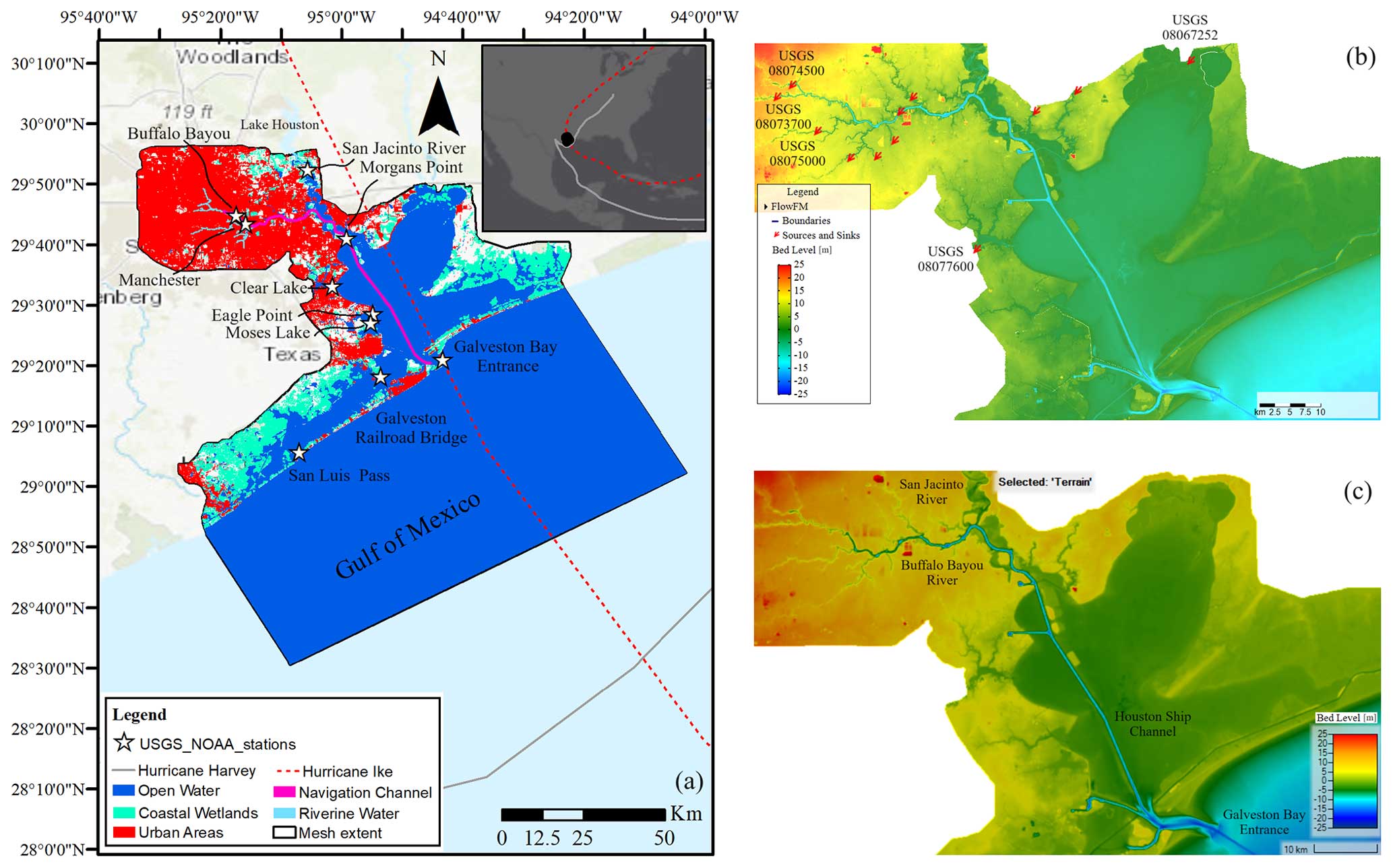
Figure 1 Model domain of Galveston Bay, TX. (a) Tide-gauge stations and land cover categories derived from the National Land Cover Database. Solid and dashed lines illustrate the best tracks of Hurricane Ike (September 2008) and Hurricane Harvey (August 2017), respectively (background map credit: Esri). Topography and bathymetry of the study area interpolated in the (b) Delft3D-FM and (c) 2D HEC-RAS models are almost identical, suggesting that the underlying mesh can capture key morphological and hydrodynamic features.

2.1 Study area

We select Galveston Bay (G-Bay) as the study area to leverage multiple spatiotemporal datasets and official reports that help calibrate and validate hydrodynamic models (Valle-Levinson et al., 2020; Sebastian et al., 2021; Rego and Li, 2010; East et al., 2008). G-Bay is the seventh largest estuary in the US and connects Houston, TX, with the Gulf of Mexico via a complex system consisting of bayous, interior bays, and rivers (Fig. 1a). G-Bay is a shallow estuary of 2 m depth, 56 km length, and 31 km width (on average) that comprises an area of approximately 1600 km². Annual average freshwater flow into G-Bay from the Buffalo Bayou river and its tributaries (USGS 08074000) and the San Jacinto River (Lake Houston's dam) is 50 and 75 m³ s⁻¹, respectively (Fig. 1b, c). Tides reaching the G-Bay entrance (NOAA 8771341) are mixed and characterized by the lunar diurnal (K₁) and principal lunar semidiurnal (M₂) constituents with tidal amplitudes of 0.15 and 0.11 m, respectively.

We simulate two CF events in G-Bay, namely, Hurricane Ike and Hurricane Harvey, that hit the Gulf of Mexico in September 2008 and August 2017, respectively (Fig. 1a). These hurricanes were selected not only because they were the most recent and relevant CF events in G-Bay but also because they were driven by dominant coastal (storm surge) and terrestrial (rainfall–runoff) flood drivers, respectively. Hurricane Ike made landfall as a Category-2 event on the Saffir–Simpson scale in the eastern part of Galveston Island, TX, on 13 September 2008. Ike produced storm surges up to 4 m near Sabine Pass and 480 mm of cumulative precipitation over southeastern TX that together led to maximum inundation depths up to 3 m a.g.l. (above ground level) in Galveston County (Berg, 2009; Rego and Li, 2010). Hurricane Harvey, on the other hand, reached Category 4 near Rockport, TX, on 24 August 2017 and made a second landfall near Cameron, LA, on 29 August 2017. Harvey generated total cumulative precipitation amounts ranging from 0.64 m up to 1.52 m over southeastern Texas and subsequent pluvial flooding in the upper river reaches of the Buffalo Bayou river with maximum inundation depths of 3 m a.g.l. (Blake and Zelinsky, 2018). In addition to heavy rainfall, a wind-driven storm surge triggered compound coastal flooding over the region that lasted 3–8 d (Valle-Levinson et al., 2020; Huang et al., 2021).

2.2 Data availability

We use publicly available data to develop and calibrate hydrodynamics models of G-Bay (Fig. 1b, c). To resemble physical conditions prior to Hurricane Ike, we consider the legacy “Galveston, Texas Coastal Digital Elevation Model” obtained from the NOAA's National Geophysical Data Center (https://www.ncei.noaa.gov/access/metadata/landing-page/bin/iso?id=gov.noaa.ngdc.mgg.dem:403, last access: 6 June 2024). This DEM includes topographic and bathymetric (topobathy) data of 2006 and is referenced to the vertical tidal datum of Mean High Water (MHW). Next, we resemble physical conditions prior to Hurricane Harvey by considering a legacy “Continuously Updated Digital Elevation Model” (CUDEM) that includes topobathy data of 2017. CUDEM is referenced to the North American Vertical Datum 1988 (NAVD88) and can be obtained from NOAA's Data Access Viewer (https://coast.noaa.gov/, last access: 6 June 2024). To account for wetland elevation errors in CUDEM, we consider a recently published coastal DEM that provides relative tidal marsh elevations over the conterminous US at a 30 m spatial resolution and referenced to the MHW datum (Holmquist and Windham-Myers, 2022). It is important to note that the coastal DEMs are referenced to the NAVD88 datum using the NOAA's Vertical Datum tool (https://vdatum.noaa.gov/, last access: 6 June 2024). Likewise, we consider land cover maps derived from the 2008 and 2016 National Land Cover Database (NLCD) as a proxy for spatially distributed roughness values for model calibration of Hurricane Ike and Hurricane Harvey, respectively (https://www.mrlc.gov/data, last access: 6 June 2024). The NLCD maps have a 30 m spatial resolution and 16 land cover classes over the continental US that can be conveniently regrouped or aggregated into general categories to avoid unnecessary specificity during model calibration.

Forcing or boundary conditions (BCs) consist of data time series of WL and river discharge that are obtained from the NOAA's Tides & Currents portal (https://tidesandcurrents.noaa.gov/, last access: 6 June 2024) and the USGS's National Water Dashboard (https://dashboard.waterdata.usgs.gov/app/nwd/en/, last access: 6 June 2024), respectively. In addition, we force the model at the ocean boundary using barotropic tides obtained from the TPXO 8.0 global inverse tide model (https://www.tpxo.net/global/tpxo8-atlas, last access: 6 June 2024). To evaluate the hydrodynamic model's performance, we leverage survey data from a temporary monitoring network deployed for Hurricane Ike, i.e., water pressure sensors (East et al., 2008), and post-flood high-water marks from the USGS's Flood Event Viewer (https://stn.wim.usgs.gov/fev/, last access: 6 June 2024) for Hurricane Harvey (Fig. 4a). Rainfall data are obtained from the rain-gauge network of the Harris County Flood Warning System (https://www.harriscountyfws.org/, last access: 6 June 2024). In addition, we use gridded data from the ERA5 reanalysis dataset to account for hourly local wind, atmospheric pressure, and total precipitation at a 30 km spatial resolution (https://www.ecmwf.int/en/forecasts/datasets/reanalysis-datasets/era5, last access: 6 June 2024). While we are aware of higher-resolution precipitation data from the NOAA's National Centers for Environmental Prediction, Harris County Flood Control District (HCFCD, https://www.harriscountyfws.org/, last access: 6 June 2024) does possess a very dense rain-gauge network (<4 km resolution). Therefore, we conduct a spatial interpolation to construct gridded precipitation data over time with a spatial resolution of 1 km. This was also proven to be effective in another peer-reviewed study in G-Bay (Sebastian et al., 2021). ERA5 rainfall data help complement HCFCD-interpolated data outside of Harris County where the mesh is coarser. Thus, any potential errors in CF modeling derived from the coarse ERA5 data are not reflected in the area of interest.

2.3 Hydrodynamic modeling

We develop hydrodynamic models using two different model software packages in order to simulate compound coastal flooding. We then analyze the uncertainty stemming from model structural inadequacy reflected in the model configuration and numerical scheme. Specifically, we set up 2D models in Delft3D-FM (version 2021.3) and HEC-RAS (version 6.3). Both models have been widely used in pluvial, fluvial, and coastal flood studies and have achieved satisfactory results (Bakhtyar et al., 2020; Liu et al., 2018; Muñoz et al., 2021; Shustikova et al., 2019). Delft3D-FM can be set up in 2D (depth-averaged) mode to solve the continuity (Eq. 1) and Reynolds-averaged Navier–Stokes equations (Eqs. 2 and 3) for incompressible fluids, uniform density, and vertical length scales that are significantly smaller that the horizontal ones (Lesser et al., 2004; Roelvink and Van Banning, 1995). In a similar way, HEC-RAS solves 2D unsteady flow, and recent model developments (e.g., version 6.3 onwards) include gridded wind and precipitation forcing input in the momentum conservation equations (USACE, 2023).

$$\begin{array}{}\text{(1)}& {\displaystyle }{\displaystyle \frac{\partial \mathit{\zeta }}{\partial t}}+{\displaystyle \frac{\partial (d+\mathit{\zeta })u}{\partial x}}+{\displaystyle \frac{\partial (d+\mathit{\zeta })v}{\partial y}}=\mathrm{0}\text{(2)}& {\displaystyle }\begin{array}{rl}{\displaystyle \frac{\partial u}{\partial t}}& +u{\displaystyle \frac{\partial u}{\partial x}}+v{\displaystyle \frac{\partial u}{\partial y}}+fv\\ & ={\displaystyle \frac{{\mathit{\rho }}_{\mathrm{a}}{C}_{\mathrm{d}}\left(U_{\mathrm{10}}-u\right)}{\mathit{\rho }(d+\mathit{\zeta })}}{\left[{\left(U_{\mathrm{10}}-u\right)}^{\mathrm{2}}+{\left(V_{\mathrm{10}}-v\right)}^{\mathrm{2}}\right]}^{\frac{\mathrm{1}}{\mathrm{2}}}\\ & -{\displaystyle \frac{\mathit{\rho }g{n}^{\mathrm{2}}}{d^{\frac{\mathrm{1}}{\mathrm{3}}}}}u{\left(u^{\mathrm{2}}+v^{\mathrm{2}}\right)}^{\frac{\mathrm{1}}{\mathrm{2}}}+v_{\mathrm{H}}\left|{\displaystyle \frac{{\partial }^{\mathrm{2}}u}{\partial x^{\mathrm{2}}}}+{\displaystyle \frac{{\partial }^{\mathrm{2}}u}{\partial y^{\mathrm{2}}}}\right|-g{\displaystyle \frac{\partial \mathit{\zeta }}{\partial x}}\end{array}\text{(3)}& {\displaystyle }\begin{array}{rl}{\displaystyle \frac{\partial v}{\partial t}}& +u{\displaystyle \frac{\partial v}{\partial x}}+v{\displaystyle \frac{\partial v}{\partial y}}-fu\\ & ={\displaystyle \frac{{\mathit{\rho }}_{\mathrm{a}}{C}_{\mathrm{d}}\left(V_{\mathrm{10}}-v\right)}{\mathit{\rho }(d+\mathit{\zeta })}}{\left[{\left(U_{\mathrm{10}}-u\right)}^{\mathrm{2}}+{\left(V_{\mathrm{10}}-v\right)}^{\mathrm{2}}\right]}^{\frac{\mathrm{1}}{\mathrm{2}}}\\ & -{\displaystyle \frac{\mathit{\rho }g{n}^{\mathrm{2}}}{d^{\frac{\mathrm{1}}{\mathrm{3}}}}}v{\left(u^{\mathrm{2}}+v^{\mathrm{2}}\right)}^{\frac{\mathrm{1}}{\mathrm{2}}}+v_{\mathrm{H}}\left|{\displaystyle \frac{{\partial }^{\mathrm{2}}v}{\partial x^{\mathrm{2}}}}+{\displaystyle \frac{{\partial }^{\mathrm{2}}v}{\partial y^{\mathrm{2}}}}\right|-g{\displaystyle \frac{\partial \mathit{\zeta }}{\partial y}}\end{array}\end{array}$$

Here, ζ is the water surface elevation (above still water), t is time, d is the water depth (below the horizontal datum or still water), u and v are the 2D depth-averaged velocities in the x and y directions, f is the Coriolis parameter, ρ_a is air density, C_d is the wind-drag coefficient, ρ is water density, U₁₀ and V₁₀ are wind velocities at 10 m height above still water in the x and y directions, g is the gravitational acceleration, n is Manning's roughness coefficient, and v_H is the horizontal viscosity parameter. Note that, unlike Delft3D-FM, HEC-RAS does not account for the atmospheric pressure term in Eqs. (1) and (2).

2.3.1 Model setup

The first hydrodynamic model is developed in Delft3D-FM using an unstructured finite-volume grid that consists of triangular cells with a spatially varying size. Unstructured grids help capture geomorphological and urban features with greater detail than conventional nested, structured grids (Kumar et al., 2009; Muñoz et al., 2022a). These features include the G-Bay entrance, artificial channels in Houston, intracoastal waterways, lateral floodplains, wetland regions, and bottleneck-like connections between G-Bay and both the Buffalo Bayou and San Jacinto rivers (Fig. 1c). Triangular cell sizes are set to increase from 3 km at the open-ocean boundary in the Gulf of Mexico up to 5 m in Harris County. This ensures a detailed simulation of CF dynamics in natural and urban settings. Similarly, the second hydrodynamic model is developed in 2D HEC-RAS using an unstructured finite-volume grid. The mesh consists of polygons of varying cell size and the numerical scheme to solve the shallow water equations is set to the Eulerian–Lagrangian (SWL-ELM) method. This, in turn, ensures that the model solves all terms in Eqs. (1)–(3), except for atmospheric pressure due to the current model capabilities of 2D HEC-RAS. In addition, we force the mesh generation with a cell size and spatial distribution similar to that of the Delft3D-FM model. Although there is no a straightforward procedure to transfer the mesh properties and/or spatial characteristics between the two hydrodynamic models, we ensure that geomorphological and urban features are correctly delineated by conducting an extensive mesh refinement in critical locations, as suggested in similar studies (Muñoz et al., 2021; Shustikova et al., 2019). The time step is controlled by the Courant–Friedrichs–Lewy condition, with a maximum value of 0.7 for both models. Also, model outputs are generated with an hourly interval for calibration and validation purposes.

After the mesh generation process, we consider multiple USGS river discharge stations in the G-Bay model as upstream BCs, including Whiteoak Bayou (USGS 08074500), Buffalo Bayou (USGS 08073700), Brays Bayou (USGS 08075000), Sims Bayou (USGS 08075500), Berry Bayou (USGS 08075605), Greens Bayou (USGS 08076000), Hunting Bayou (USGS 08075770), Vince Bayou (USGS 08075730), Clear Creek (USGS 08077600), Goose Creek (USGS 08067525), Cedar Creek (USGS 08067500), and Trinity River (USGS 08067252). Also, due to the lack of available river-gauge stations located immediately downstream of Lake Houston dam, river flow from Lake Houston dam to the San Jacinto River is estimated as the sum of upstream freshwater input to the lake (Fig. 1). Such an estimation is realistic because the dam is not operating as a flood control structure anymore and was overflowed by extreme river discharge as a result of Hurricane Harvey (Sebastian et al., 2021; Valle-Levinson et al., 2020). Regarding the downstream BCs, we force the G-Bay model with storm tides using WL records from two tide-gauge stations, namely, Freeport Harbor (NOAA 8772471) and Galveston Bay Entrance (NOAA 8771341). These stations are located offshore and are a good proxy for coastal WL propagating from the open-ocean boundary. To account for WL variability arising from atmospheric variables, we include reanalysis data of 10 m wind velocity and atmospheric (sea level) pressure in the model simulations. Note that the latest versions of 2D HEC-RAS allow the user to simulate wind speeds even though the atmospheric pressure component is yet to be implemented in Eqs. (2) and (3).

Lastly, we retrieve rainfall data from a relative dense rain-gauge network of the Harris County Flood Warning System. These data have been validated and further used to estimate flood damages in G-Bay (Sebastian et al., 2021). In addition, we complement these data with “total precipitation” reanalysis datasets from ERA5 in order to estimate rainfall patterns in coastal areas beyond Harris County and over the Gulf of Mexico (Fig. 1). Specifically, we use the “inverse distance weight” as the interpolation method in ArcGIS with an output cell size of 1 km (e.g., shortest Euclidean distance between existing rain gauges), a search radius of 5 points, and a power function of 2. The interpolation method as well as the aforementioned values follow those suggested in other studies and are validated through sensitivity analysis (Sebastian et al., 2021; Ahrens, 2006; Otieno et al., 2014).

2.3.2 Model calibration

G-Bay is influenced by multiple flood drivers, including local rainfall, river discharge, and storm tides. At low river flow rates, tides propagate from the ocean boundary in the landward direction where they attenuate and eventually vanish due to bottom friction (Hoitink and Jay, 2016; Bolla Pittaluga et al., 2015). Therefore, we ensure that the model setup (Sect. 2.3.1) is adequate to simulate tidal propagation across the model domain. Specifically, we simulate tidal dynamics in Delft3D-FM by setting barotropic tides from the TPXO 8.0 global inverse tide model as forcing data at the open-ocean boundary (Egbert and Erofeeva, 2002). We then run 100 ensemble model realizations for a 1-year simulation window without incorporating any additional forcing (e.g., only tides) and considering a range of plausible Manning's roughness values (n) derived from pertinent literature and technical reports (Liu et al., 2018; Arcement and Schneider, 1989). A combination of plausible n values are generated with the Latin hypercube sampling (LHS) technique (Helton and Davis, 2003) and evaluated via ensemble model simulations in a high-performance computing (HPC) system (Table 1). We next identify an optimal (calibrated) value for the “open water” category that achieves the lowest root-mean-square error (RMSE) and mean absolute error (MAE) as well as the highest Kling–Gupta efficiency (KGE) and Nash–Sutcliffe efficiency (NSE). These metrics and underlying equations have been presented in another study on G-Bay (Muñoz et al., 2022a).

Table 1 Manning's roughness values tested for model calibration in Delft3D-FM/2D HEC-RAS.

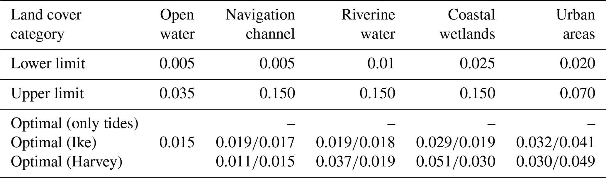
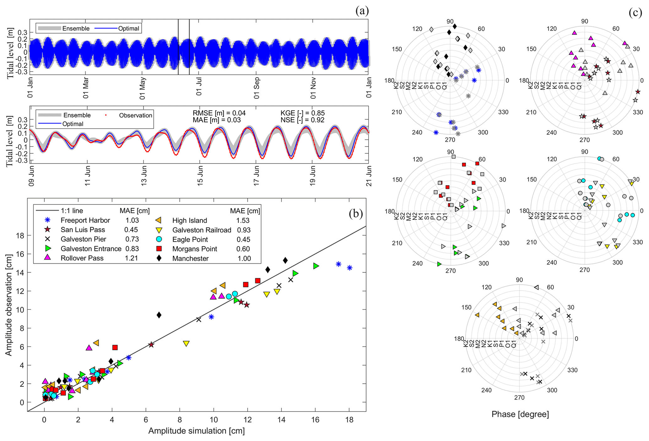
Figure 2 Evaluation of tidal propagation in Galveston Bay. (a) Ensemble and optimal model simulation of tides for a 1-year window and a close-up section (vertical lines) showing the observed tidal levels. Results of harmonic analysis show (b) tidal amplitudes (1:1 line) and (c) tidal phase for selected tidal constituents (concentric circles). Each colored marker represents a tide-gauge station with the underlying tidal constituents, whereas gray markers represent observed tidal phases.

Furthermore, we conduct harmonic analyses and retrieve tidal amplitudes and phases for the main tidal constituents in G-Bay including K2, S2, M2, N2, K1, S1, P1, O1, and Q1 (NOAA, 2000). We then compare observed and simulated tidal characteristics at each tide-gauge station using a 1:1 line assessment as well as concentric circles. In general, the evaluation metrics suggest that the model setup is adequate to simulate tidal propagation in G-Bay. Also, the optimal n value for open water helps minimize both the RMSE and MAE and achieve high NSE and KGE scores (Fig. 2a). The 1:1 line shows a satisfactory agreement between observed and simulated tidal amplitudes, with a maximum MAE of 1.53 cm (Fig. 2b). Likewise, observed and simulated tidal phases are in good agreement for the majority of tidal constituents and stations in G-Bay. The closer the colored (simulated) and gray (observed) markers in each concentric circle, the more accurate the simulated phase. Note that we only evaluate tidal propagation using the Delft3D-FM model because this software is installed in our HPC system, whereas 2D HEC-RAS is run on a desktop computer. Moreover, the former model can run in parallel, whereas recent 2D HEC-RAS versions in Linux run in series within the HPC system. Thus, the latter would require significantly more computational resources and time to accomplish 100 ensemble model realizations for a 1-year simulation window. Nevertheless, we expect similar score metrics regarding tidal propagation for a 1-year simulation window, as the model setup of 2D HEC-RAS is similar to that of Delft3D-FM (i.e., mesh extent, refinement regions, and cell size grid. Also, we support this claim based on calibration and validation results of CF events as explained later on, i.e., Hurricane Ike and Harvey.

Next, we calibrate n values of the navigation channel, riverine water, coastal wetlands, and urban areas for Hurricane Ike and Hurricane Harvey (Table 1). We follow an identical process to identify optimal n values for both the Delft3D-FM and 2D HEC-RAS models, i.e., LHS technique with 100 ensemble members, but this time we keep the calibrated n value for the “open water” category invariant to ensure accurate tidal propagation. It is worth noting that both models are independently calibrated in order to ensure a reliable assessment of model parameters and model structure errors, especially in riverine areas in Houston. The roughness coefficient of open water is common for both models, as it simulates tidal propagation from the ocean boundary. Also, we set a 1-month warm-up period for the model to reach equilibrium and consider a 1-week simulation window (centered on the peak WL) to assess the accuracy of model simulations (Fig. 3 and Figs. S1 and S2 in the Supplement). In general, both hydrodynamic models perform satisfactorily, especially at downstream tide-gauge stations where the RMSE is below 0.30 cm. However, the RMSE progressively increases at upstream tide-gauge stations due to a relatively large riverine influence and underlying nonlinear interactions with storm tides (Fig. 3d, h). The latter is more evident in model simulations of Hurricane Harvey, as the peak river discharge at the Buffalo Bayou station (USGS 08073700), located upstream of the Manchester tide-gauge station (NOAA 8770777), is 3.5 times higher than that of Hurricane Ike. Also, inaccuracies in the topobathy data along the Buffalo Bayou river and its tributaries might have reduced the model's performance in the upstream part of G-Bay, as reported in flood hazard and damage studies (Wing et al., 2019; Jafarzadegan et al., 2021a; Valle-Levinson et al., 2020).

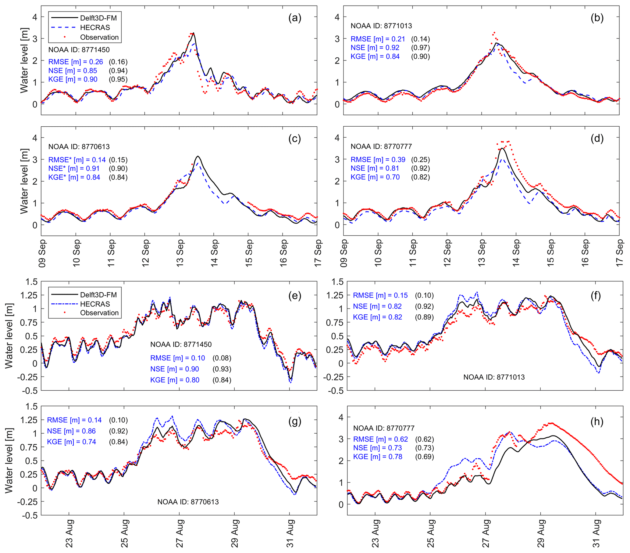
Figure 3 Model calibration at selected tide-gauge stations in Galveston Bay. Model performance is evaluated in terms of the RMSE, NSE, and KGE for (a–d) Hurricane Ike and (e–h) Hurricane Harvey. The color code indicates score metrics for Delft3D-FM (black) and 2D HEC-RAS (blue).

2.3.3 Model validation

To validate the hydrodynamic models, we generate composite maps representing maximum WLs within the simulation period of Hurricane Ike and Hurricane Harvey and compare those maps against USGS's high-water marks collected in the aftermath of both hurricanes (Fig. 4a). We evaluate the accuracy of the composite maps by comparing observed and simulated maximum WLs (Fig. 4b). Data points that fall along the 1:1 (diagonal) line represent a perfect match between those maximum WLs. The validation process indicates that Delft3D-FM and 2D HEC-RAS produce maximum WLs that are in close agreement with available high-water marks in G-Bay; moreover, both the RMSE and MAE agree well with the corresponding metrics reported in similar CF studies (Huang et al., 2021; Lee et al., 2024; Sebastian et al., 2021; Wing et al., 2019). In addition, we validate peak WLs at selected tide-gauge stations (Figs. 3, S1, S2) with respect to CF hazard maps generated in Delft3D-FM for Hurricane Ike and Hurricane Harvey (Fig. 4c and d, respectively). Note that we mask out values below 0.10 m in order to enhance visualization of water depths above ground. As expected, the peak WL of Hurricane Ike (∼3 m) triggers a relatively large flood extent and water depth in the lower part of G-Bay, whereas the peak WL of Hurricane Harvey (∼1.25 m) produces moderate coastal flooding over the same area. However, flood extent and water depth in Harris County are relatively large compared with those triggered by Hurricane Ike due to the compounding effects of heavy rainfall, extreme river discharge, and storm tides. Such compounding effects are evident at Manchester tide-gauge station where freshwater input controls WL dynamics starting on 27 August (Fig. 3h). Also, note that Delft3D-FM constantly outperforms 2D HEC-RAS based on the evaluation metrics and 1:1 line assessment (Figs. 3, 4). Following this, we hereinafter consider Delft3D-FM as the best hydrodynamic model to analyze cascading uncertainty in G-Bay with respect to 2D HEC-RAS.

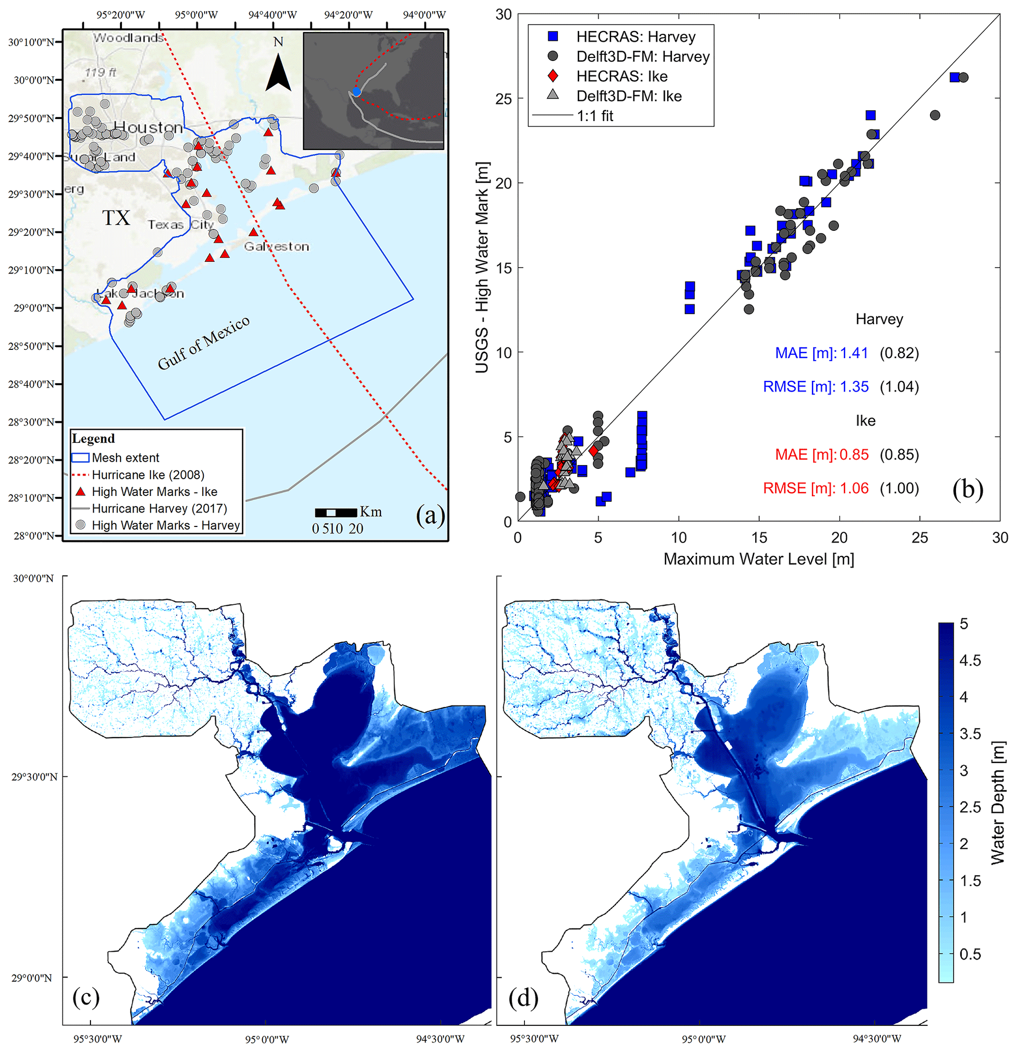
Figure 4 Validation of the Delft3D-FM and 2D HEC-RAS models in Galveston Bay. (a) Spatial distribution of the high-water marks collected in the aftermath of CF events by the USGS (background map credit: Esri). (b) Validation of composite maps with respect to the USGS high-water marks. Score metrics are calculated for 2D HEC-RAS and Delft3D-FM (in parentheses). CF hazard maps represent maximum water depths computed with Delft3D-FM and corresponding to (c) Hurricane Ike and (d) Hurricane Harvey.

2.3.4 Model scenarios

We propose five scenarios to analyze the effects of isolated and total uncertainty on CF hazard assessment for Hurricane Harvey (Table 2). The first scenario focuses on the initial condition of the system, including topographic and bathymetric data in coastal DEMs. Recently, Holmquist and Windham-Myers (2022) produced a DEM of relative tidal marsh elevation for the conterminous US using land cover classes derived from the 2010 Coastal Change Analysis Program (C-CAP). As this DEM accounts for elevation errors within coastal wetlands, we conveniently evaluate uncertainty from the initial condition of the system using the aforementioned DEM and NOAA's CUDEM in hydrodynamic simulations (see Sect. 2.2). The second scenario represents uncertainty derived from forcing conditions that are often neglected in real-time hurricane-induced flood forecasts and advisories (CERA, 2023). Specifically, such flood forecasts assume that riverine flow and local rainfall contributions to flooding are relatively small compared with those driven by storm surge. Following this reasoning, we will analyze the impact of local rainfall and riverine flow in CF dynamics by turning off those two forcing conditions in hydrodynamic simulations.

Table 2 Model scenarios for simulating isolated and total uncertainty in G-Bay.

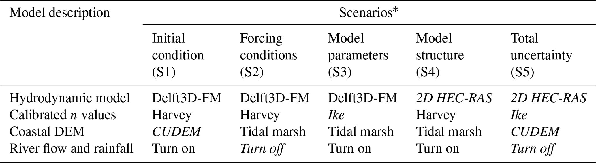
^* Italic text denotes changes with respect to the best model setup for simulating Hurricane Harvey.

The third scenario analyzes uncertainty stemming from model parameters, including bed channel and floodplain roughness coefficients associated with land cover classes from the NLCD (Fig. 1a, Table 1). Here, we simulate compound coastal flooding triggered by Hurricane Harvey using two sets of optimal (calibrated) n values. The first set consists of n values calibrated for Hurricane Ike (September 2008), whereas the second set comes from the actual model calibration of Hurricane Harvey (August 2017). The reasoning is that a realistic estimation (or proxy) of calibrated n values for future flood scenarios consists of those already calibrated for past flood events (Domeneghetti et al., 2013; Meresa et al., 2021). In this regard, Hurricane Ike is the closest and most relevant CF event that impacted G-Bay prior to Hurricane Harvey. The fourth scenario represents uncertainty derived from model structure, including the model setup and configuration necessary to simulate flood extent and inundation depth. Therefore, we analyze this source of uncertainty by comparing model outputs of Delft3D-FM and 2D HEC-RAS (see Sect. 2.3). Lastly, the fifth scenario is named “total uncertainty” and involves all sources of uncertainty including their cascading effect on CF hazard assessment.

2.4 Regression models

The proposed model scenarios are further modified to quantify their relative contribution to total uncertainty using regression models. Here, we report uncertainties in terms of WL residuals computed between each scenario and the best model setup for simulating Hurricane Harvey. Such a model setup consists of the calibrated Delft3D-FM model that accounts for elevation errors within coastal wetlands and additionally incorporates the effects or river flow and local rainfall in CF modeling (Figs. 3, 4). As 2D HEC-RAS generates raster-based flood maps, we extract WLs at each grid node of Delft3D-FM to compute the corresponding WL residuals. This helps ensure consistency in uncertainty analysis over the model domain. Also, note that WL residuals evolve in time and space, and their magnitude attributed to the sources of uncertainty is represented by the four model scenarios. Therefore, we first compute the maximum WL residual across the model domain for the entire simulation period (e.g., 10 d window) as well as time-evolving residuals with an interval of 6 h. This time interval is set to comply with the timing of hurricane advisories of the National Hurricane Center and, thus, enable the construction of 40 datasets within the 10 d simulation window, i.e., WL forecasts and advisories every 6 h.

2.4.1 Multiple linear regression

WL residuals obtained from physically based model simulations are used as input features for multiple linear regression (MLR) and nonlinear models (Fig. 5). First, we fit the input features using an MLR model and considered it as a benchmark model to further evaluate the benefits of nonlinear models including physics-informed machine learning (PB–ML). The goal of the MLR model is to estimate total uncertainty as the target variable in terms of WL residuals. As we are dealing with WL residuals in meters that have a comparable order of magnitude, we do not scale or normalize the input features prior to the fitting process. This is also convenient for the evaluation purposes of the fitted model and the relative importance quantification of each source of uncertainty based on fitted regression weights. We do, however, identify and remove outliers in the input features, especially those arising at the edges of the mesh and those around the BCs. We use the “statsmodels API” package in Python to conduct a robust fitting of input features (https://www.statsmodels.org/stable/api.html, last access: 6 June 2024) and report regression coefficients with the underlying statistical significance and confidence intervals (see Sect. 3.2).

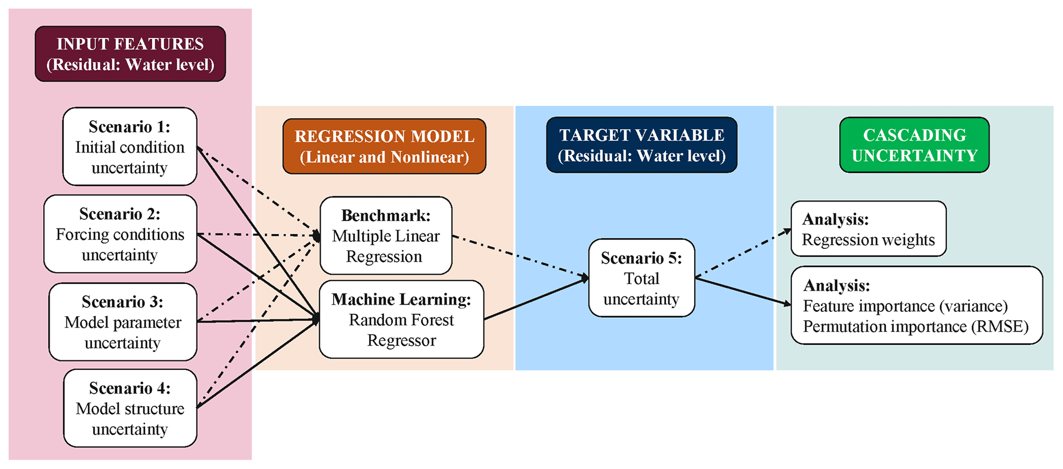
Figure 5 Schematic of multiple linear regression and process-based machine learning models to quantify cascading uncertainty. Input features and target variable are reported in terms of water level residuals derived from hydrodynamic simulations of Hurricane Harvey. The target variable contains all sources of uncertainty and their implicit cascading effects.

2.4.2 Linked process-based and machine learning models

We conducted a preliminary analysis to identify the best nonlinear ML model that predicts total uncertainty (not shown here for brevity). Among those models, we notice that a random forest regressor model outperforms support vector machine and artificial neural networks (e.g., multiple-layer perceptron model), and the latter agrees with results of multiple flood studies (Chen et al., 2020; Mosavi et al., 2018; Schoppa et al., 2020). Random forest (RF) is a nonparametric ensemble algorithm that builds multiple decision trees based on random bootstrapped samples through replacement (Breiman, 2001). The advantage of RF over other nonlinear regression models lies in its simplicity and easy implementation for efficient regression and classification tasks. Also, RF connects input and target features with complex and nonlinear associations and provides estimates of feature importance to predict the target variable (Alipour et al., 2020; Wang et al., 2015). We develop an RF regressor model and conduct a thorough model evaluation in Python using the “scikit-learn” package. WL residuals from each scenario are set as input (S1–S4) and target (S5) features, and our analysis is focused on both time-evolving and maximum residuals across the model domain. We split input features into training (80 %) and validation (20 %) datasets using the total number of data points after outlier removal. In the context of hydrodynamic modeling, outliers are unrealistic WLs emerging around upstream and downstream BC lines as well as the edges of the model domain. Such values are extreme values, either positive or negative, that do not reflect WL dynamics within the model domain. Therefore, we masked out such values using a buffer polygon in ArcGIS and proceeded with the training and validation dataset using realistic WLs (e.g., 1 093 501 data points). Those data points represent the number of grid nodes generated in Delft3D-FM (see Sect. 2.3.1). Next, we conduct hyperparameter tuning to build decision trees and estimate optimal (calibrated) values for each parameter using an HPC system (Table 3).

Table 3 Hyperparameter grid and optimal (calibrated) parameter values for the RF regressor model.

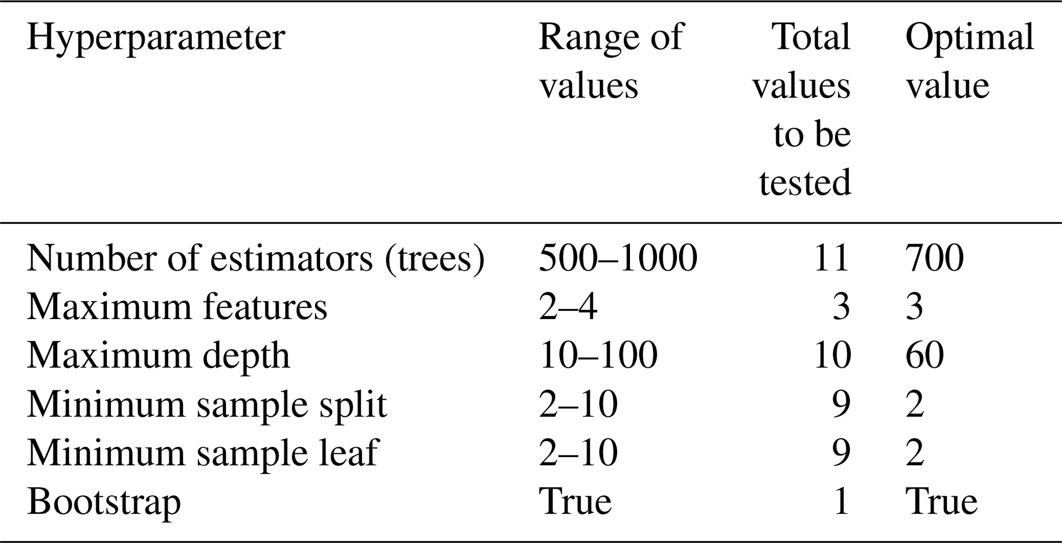
We use the scikit-learn package to find optimal values and also account for overfitting issues through a cross-validation (CV) process. For this, we generate an initial grid of parameter values within a specified range using the LHS technique (Helton and Davis, 2003). Then, we use a “k-fold” approach to conduct CV using the training dataset. The number of k-folds is set to five, and the parameter grid is generated with a fixed seed value to ensure reproducibility. We then use the grid in the “RandomizedSearchCV” function to randomly sample a set of hyperparameter values and conduct a k-fold CV for each combination of values. The number of combinations to be tested is defined by the “n_iter” parameter that is set to 100 here. We repeat the splitting and sampling process for time-evolving WL residuals and conduct hyperparameter tuning for the resulting 40 datasets using the HPC system. Nevertheless, we notice that the optimal values associated with each dataset and those reported in Table 3 lead to similar score metrics in the validation dataset (e.g., R², R, KGE, and RMSE). Also, the main differences in the score metrics are observed in the third or fourth decimal place (see Sect. 3.2).

3 Results and discussion

3.1 Effects of isolated and total uncertainty

Scenarios S1 to S4 are designed to analyze the effect of each source of uncertainty on CF hazard assessment (Figs. 6, S3). We conveniently display maximum WL residuals across the model domain where positive or negative values indicate an overestimation or underestimation of WLs, respectively. Scenario S1 accounts for elevation errors in lidar-derived DEMs that lead to a complex heterogenous pattern with both over- and underestimation of maximum WL residuals (Fig. 6a, b). This scenario displays an overestimation of WLs in the tributaries of the Buffalo Bayou river, the Houston and Galveston navigation channels, and intracoastal waterways in the lower part of G-Bay. Such an overestimation can be explained by inconsistencies in bathymetric data between the tidal marsh DEM and NOAA's CUDEM. In addition, this scenario shows an underestimation of WLs in the upper part of G-Bay, including the head of the Buffalo Bayou's tributaries and the San Jacinto River that is surrounded by coastal wetlands (Fig. 1a). Wetlands are natural buffers that dissipate extreme WLs and attenuate storm surge with a rate of 1.7–25 cm km⁻¹ depending on marsh height, biomass, and storm characteristics (Alizad et al., 2018; Kumbier et al., 2022; Leonardi et al., 2018). As expected, there is a consistent underestimation of WLs due to vertical adjustments that lower wetland elevation in the tidal marsh DEM (e.g., with respect to that of CUDEM), reduce wetlands' buffer capacity, and increase WLs.

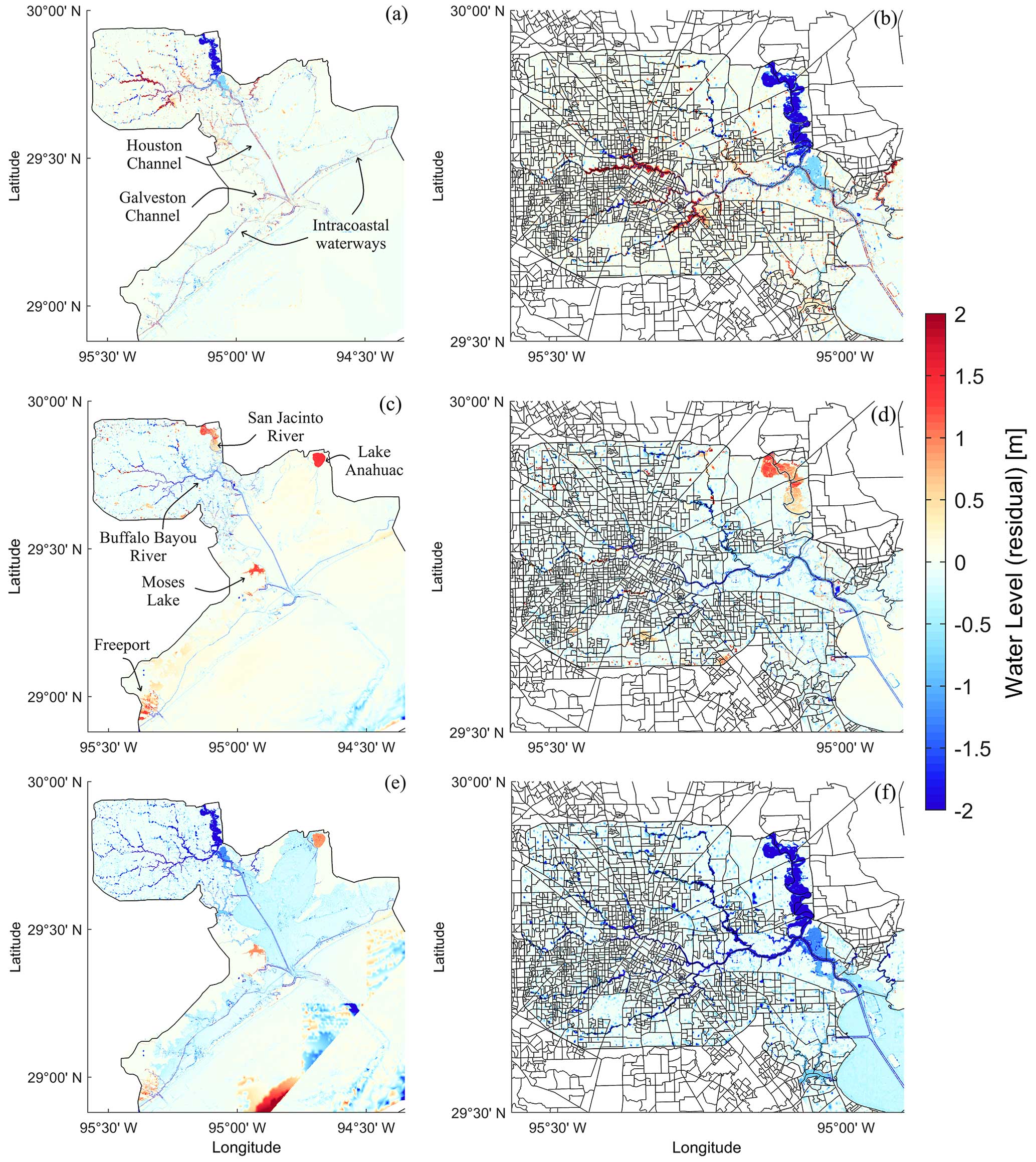
Figure 6 Effect of isolated and total uncertainty on compound flood hazard assessment in Galveston Bay. Maximum water level residuals represent model scenarios with uncertainty stemming from the (a, b) initial condition, (c, d) model structure, and (e, f) total uncertainty. Water level residuals are calculated with respect to the best hydrodynamic model calibrated for Hurricane Harvey. Positive and negative residuals indicate overestimation and underestimation across the model domain, respectively. Panels (b), (d), and (f) show a close-up window over block census groups in Harris County on the northwest side of Galveston Bay.

Scenario S2 focuses on uncertainty derived from forcing conditions including river flow and local rainfall. This scenario leads to an underestimation of WLs across the model domain (Fig. S3a, b). The effect of neglecting forcing conditions on CF hazard assessment is more evident on the northwest side of G-Bay where CF was driven by heavy rainfall and extreme river flow triggering urban flooding in Harris County. In fact, Hurricane Harvey caused urban flooding in Houston city due to an unprecedent rainfall depth greater than 1.5 m as well as an extreme river flow conveyed by the Buffalo Bayou and San Jacinto rivers (Blake and Zelinsky, 2018; Sebastian et al., 2021; Valle-Levinson et al., 2020). Scenario S3 analyzes the influence of model parameters that are conventionally calibrated for historical flood events (e.g., Hurricane Ike) and used as a proxy for simulating future flood events (Domeneghetti et al., 2013; Meresa et al., 2021). This scenario exhibits an overestimation of WLs that is particularly evident on the northwest side of G-Bay (Fig. S3c, d). Such an overestimation can be related to the peak WL of Hurricane Ike (∼3 m) and Hurricane Harvey (∼1.25 m) as well the corresponding calibrated (optimal) n values (Table 1). In general, the n values calibrated for Hurricane Ike are lower in magnitude than those for Hurricane Harvey; thus, they are more effective with respect to reducing bed friction and tidal damping (Bhola et al., 2019; Liu et al., 2018; Mayo et al., 2014; Pappenberger et al., 2005). Consequently, considering the low n values calibrated for Hurricane Ike to simulate Hurricane Harvey leads to an overestimation of the storm tide that propagates from the open-ocean boundary to the upper part of G-Bay. Note that the peak WL of Hurricane Ike is 2.4 times larger than that of Hurricane Harvey, and its effect is observed in the maximum WL residuals in the Buffalo Bayou's tributaries.

Scenario S4 accounts for uncertainty derived from the model structure and capabilities of 2D HEC-RAS compared with those of Delft3D-FM. This scenario leads to a complex heterogenous pattern with both over- and underestimation of maximum WL residuals across the model domain (Fig. 6c, d). Specifically, this scenario displays an overestimation of WLs in the San Jacinto River, Moses and Anahuac lakes, and Freeport, whereas it results in an underestimation in Harris County, the Buffalo Bayou river and its tributaries, the Houston and Galveston navigation channels, and intracoastal waterways in the lower part of G-Bay. This complex pattern highlights the capability (or inability) of the hydrodynamic models to account for atmospheric pressure in the conservation of momentum (Eqs. 2 and 3) and to capture coastal geomorphological and urban features in the mesh generation process, i.e., structured vs. unstructured grids (Bates, 2022, 2023).

Lastly, scenario S5 is named total uncertainty because it accounts for the isolated and cascading effects of the sources of uncertainty on spatiotemporal CF hazard assessment (Fig. 6e, f). This scenario displays an overall underestimation of maximum WL residuals on the northwest side of G-Bay, which is similar to the pattern observed in scenario S2 (e.g., forcing conditions). Likewise, it displays both over- and underestimation of WL residuals in the lower part of G-Bay, resembling the patterns of scenarios S4 and S1, respectively (e.g., model structure and input data). In contrast, the overestimation pattern of scenario S3 is not visually reflected in scenario S5. This discrepancy is explained in the following section.

3.2 Relative contribution of isolated and cascading uncertainty

3.2.1 Compound flood hazard assessment

We fit and train MLR and ML models using maximum WL residuals as an indicator of CF hazard in G-Bay (Table 4). Regression weights are statistically significant for all four scenarios (p value < 0.05), including S3 in spite of the negative correlation. Also, the Pearson and Kendall correlation coefficients reveal a statistically significant linear correlation between total uncertainty and isolated uncertainty (Fig. 7). Note that the rank of such correlations, in descending order, agrees well with the maximum WL residuals and underlying patterns resulting from the model scenarios (Fig. 6). Among them, uncertainty stemming from model parameters has a negative linear correlation with total uncertainty that partially explains the discrepancy of residual patterns already mentioned in the previous section. Particularly, a negative correlation suggests that an increase in WL residuals from scenario S3 results in a decrease in those from scenario S5. Note that the MLR model estimates total uncertainty with a relatively high accuracy, as corroborated by the score metrics, i.e., R²=0.76, R=0.87, RMSE = 0.42 m, and KGE = 0.82 (Fig. 7c).

Table 4 Multiple linear regression fitting on maximum water level residuals.

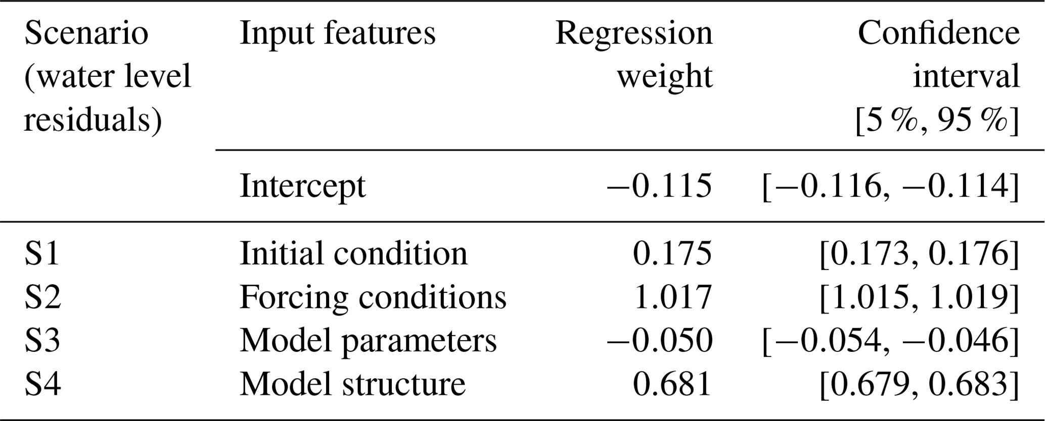
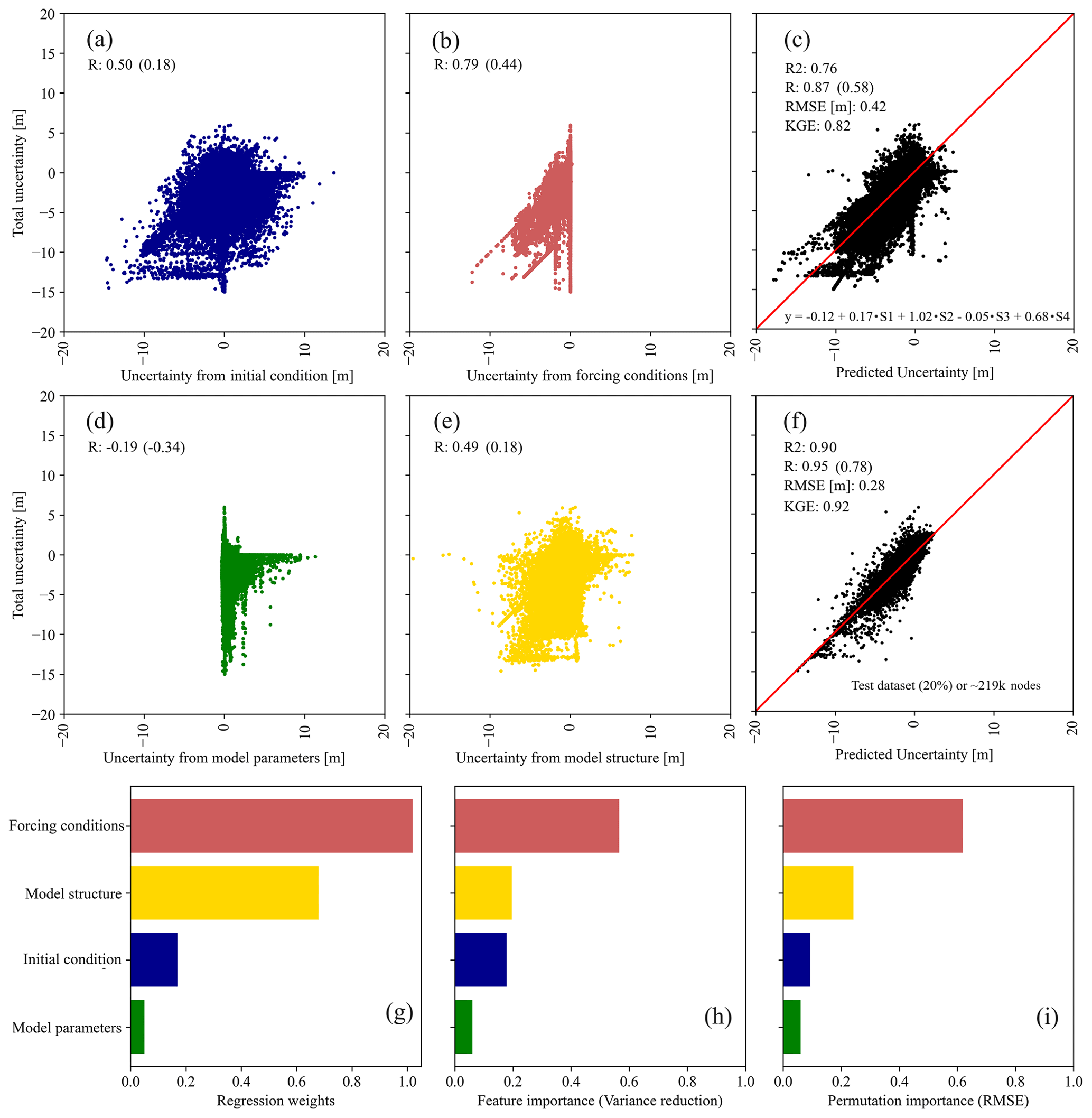
Figure 7 Isolated and total uncertainty reported in terms of water level residuals (in meters). (a, b, d, e) Linear associations with the corresponding Pearson's and Kendall's correlation coefficients, with the latter in parentheses. (c, f) Total and predicted uncertainty obtained from multiple linear regression and RF regressor models. (g–i) Relative contribution of the initial condition, forcing conditions, model parameters, and model structure to total uncertainty in terms of regression weights and feature and permutation importance.

Confidence intervals are obtained from the statsmodels API package available in Python.

Overall, the absolute magnitude of regression weights agrees well with the rank resulting from either Pearson's or Kendall's correlation coefficients. This suggests that uncertainty stemming from the forcing conditions and model structure are crucial for estimating total uncertainty in CF hazard assessment (Fig. 7g). Other flood studies have shown similar results and demonstrated that uncertainty stemming from forcing conditions is even more important than that of the remaining sources, especially for flood prediction and inundation mapping in riverine systems (Alipour et al., 2020; Jafarzadegan et al., 2023; Pappenberger et al., 2008; Savage et al., 2016). The initial condition of the system and model parameters are also relevant sources of uncertainty, but they show a relatively low regression weight. Note that if WL residuals of scenarios S1, S3, and S4 are kept invariant, any perturbations of scenario S2 will result in a nearly identical response of scenario S5 as well as a negative offset of 12 cm. Although MLR models help analyze the influence of each input feature to estimating total uncertainty, they do not capture hidden associations and/or interactions among the input features. This, in turn, reduces the effectiveness of MLR models to characterize cascading effects on total uncertainty.

To overcome this limitation, we determine whether or not the proposed PB–ML model (e.g., RF regressor) outperforms the MLR model based on the aforementioned evaluation metrics. In this regard, the score metrics evince a substantial improvement by the PB–ML model: the RMSE decreases to 0.28 m, whereas R², R, and the KGE increase up to 0.90, 0.95, and 0.92, respectively (Fig. 7f). Next, we conduct a rank analysis focused on the contribution of each input feature to the model's variance reduction and overall performance for total uncertainty estimation (Fig. 7h and i, respectively). In the proposed RF regressor model, feature importance measures the mean decrease in variance within each selected decision tree, whereas permutation importance measures the decrease in a predefined score metric when individual input features are randomly shuffled (Breiman, 2001). Specifically, the four input features are shuffled multiple times and the RF regressor model is refitted to estimate their importance in the model's performance. Here, we shuffle the input features 100 times and set the RMSE as the evaluation metric to be consistent with the ensemble members and score metrics used in the calibration and validation process (see Sect. 2.3.2). Notably, the rank of feature importance agrees well with that of the regression weights, indicating that the forcing conditions are not only the main contributor to total uncertainty in CF hazard assessment (56 %) but also a key feature for variance reduction (Fig. 7h). It is noted that the model structure, the input conditions, and the model parameters contribute 20 %, 18 %, and 6 % to the variance reduction, respectively.

The advantage of permutation over feature importance analysis is that the former method circumvents any overfitting issues by focusing the analysis on validation data (∼219 000 data points). Also, permutation importance is not biased towards input features with a large number of unique values, compared with feature importance, i.e., high cardinality. Nevertheless, note that we address potential issues of overfitting and high cardinality through a 5-fold CV process in the training process (see Sect. 2.5.2). Similarly, the rank of permutation importance agrees well with both the ranks of regression weights (or slope terms) and those derived from feature importance (Fig. 7i). Nevertheless, note that the permutation importance of forcing conditions (61 %) is higher than that of feature importance; this can be partially explained by the number of data points used in the computation of the corresponding importance as well as the objective function, i.e., training vs. test datasets and mean variance decrease vs. RMSE. Note that model structure, input, and parameters contribute 24 %, 9 %, and 6 % to the overall model performance, respectively. Following these results, we recommend that any efforts to improve CF modeling and hazard assessment should focus on accounting for all relevant forcing (boundary) conditions and implementing a suitable hydrodynamic model to simulate complex compound coastal flood dynamics. For example, recent studies have shown that estimating water deficits between upstream and downstream flows and distributing such deficits using lateral flows and vertical fluxes (as additional forcing conditions) improve the performance of flood modeling during extreme events (Jafarzadegan et al., 2021b; Oruc Baci et al., 2024).

3.2.2 Compound flood modeling

We track the trajectory of the four sources of uncertainty during the onset, peak, and dissipation of Hurricane Harvey using a 6 h interval for the entire simulation period (Fig. 8a). For this, we fit MLR and train PB–ML models for each of the 40 datasets containing WL residuals and report relative and cumulative contributions as well as models' performance in terms of the R², R, KGE, and RMSE. The model structure and initial condition of the system are the main sources of total uncertainty at the onset of Hurricane Harvey with a contribution of 60 % and 20 %, respectively (Fig. 8b). However, their relative contribution drops around the peak WL because forcing conditions become a more relevant source of uncertainty until the dissipation of WLs, i.e., drastic increase from 10 % to 50 %. The contribution of model parameters is estimated at 10 % and remains almost invariant during the onset, peak, and dissipation of Hurricane Harvey. Furthermore, the cumulative contribution of each source of uncertainty helps visualize their overall importance for total uncertainty estimation in the simulation period (Fig. 8d). In contrast to the rank of contributions established for maximum WL residuals (see Sect. 3.2.1), note that the model scenario and/or input feature derived from model structure is the main contributor to variance reduction in the RF regressor model (49 %) followed by that of the forcing conditions (23 %), initial condition (20 %), and model parameters (8 %).

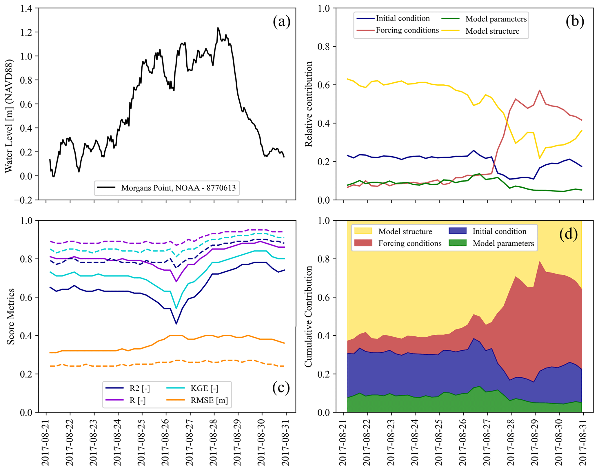
Figure 8 Evolution of water level residuals as a proxy for total uncertainty during the onset, peak, and dissipation of Hurricane Harvey. (a) Observed water levels at Morgans Point station located in the middle of G-Bay. (b) Relative contribution of the initial condition, forcing conditions, model parameters, and model structure to variance reduction in total uncertainty estimation. (c) Evolution of the R², R, KGE, and RMSE in the simulation window, with solid and dashed lines representing multiple linear regression and RF regressor models, respectively. (d) Cumulative contribution of the four main sources of uncertainty. The area under the curves represents the average contribution to variance reduction for the entire CF event.

These results are somehow similar to other studies that analyzed how the influence of forcing (boundary) conditions and model parameters change during flood events (Alipour et al., 2022; Jafarzadegan et al., 2021b; Savage et al., 2016). Although those studies identify forcing conditions as the most influential factor for flood inundation mapping, uncertainty stemming from model structure is not explicitly analyzed; however, it is recognized as a determinant factor of the results. Lastly, the evaluation metrics computed for the 40 datasets indicate that RF regressor models (dashed line) outperform the benchmark MLR models (solid line) in the simulation period (Fig. 8c). Note that the R², R, and KGE display a sudden drop around the peak WL, suggesting that MLR models cannot fully characterize total uncertainty, whereas the same evaluation metrics of RF regressor models remain almost invariant due to the ability of nonlinear models to capture any complex interactions as well as cascading effects arising from the four sources of uncertainty. Likewise, note that the RMSE drops to ∼11 cm when characterizing cascading uncertainty with RF regressor models. Also, there is a rather constant RMSE of ∼25 cm when estimating total uncertainty in terms of WL residuals in the simulation period.

4 Conclusions

In the present study, we characterize isolated and cascading uncertainty during the onset, peak, and dissipation of Hurricane Harvey in Galveston Bay, TX. For this, we develop two hydrodynamic models (e.g., Delft3D-FM and 2D HEC-RAS) to simulate compound coastal flooding and conduct compound flood (CF) hazard assessment. The calibrated and validated models help simulate a set of scenarios that reflect uncertainties stemming from the initial condition, forcing conditions, model parameters, and model structure. We then train a physics-informed machine learning model (PB–ML) to estimate total uncertainty in terms of water level (WL) residuals and evaluate the model's performance with respect to a benchmark multiple linear regression (MLR) model. The effects of isolated uncertainty on CF hazard assessment match the spatial patterns observed in the total uncertainty scenario across the model domain, especially for the scenarios that reflect uncertainty from the initial condition of the system, forcing conditions, and model structure. Conversely, the scenarios representing total uncertainty and that from model parameters exhibit a negative correlation, resulting in a discrepancy of spatial patterns across the model domain. Nevertheless, we estimate that the forcing conditions, model structure, initial condition, and model parameters contribute to 56 %, 20 %, 18 %, and 6 % of variance reduction in the PB–ML model, respectively. These values agree well with the rank of regression weights estimated with the MLR regression model, helping support the conclusion that the forcing (boundary) condition is the main contributor to total uncertainty in CF hazard assessment.

Regarding CF modeling, we observe an interplay of relative importance where model structure and the initial condition of the system are the main sources of total uncertainty at the onset of Hurricane Harvey. However, their relative importance drops around the peak WL because forcing conditions become a more relevant source of uncertainty until the dissipation of WLs. Also, the importance of model parameters remains almost invariant during the onset, peak, and dissipation of Hurricane Harvey. Nonetheless, model structure is the main contributor to variance reduction (49 %) followed by the forcing conditions (23 %), initial condition (20 %), and model parameters (8 %). Lastly, MLR models are not suitable to characterize total uncertainty, as their performance is sensitive to the peak WL, as evinced in the evaluation metrics (e.g., RMSE, R², R, and KGE). Conversely, PB–ML models are less sensitive to changes in WL dynamics due to their ability to capture hidden interactions and cascading effects arising from the four sources of uncertainty. Following these results, we conclude that PB–ML models are a feasible alternative to conventional statistical methods for characterizing cascading uncertainty in compound coastal flood modeling and CF hazard assessment. The relative importance of the sources of uncertainty may also vary depending on catchment properties, storm characteristics, and dominant flood drivers, i.e., coastal-to-inland transition zones. Ongoing work is being conducted to effectively reduce uncertainty using residual learning techniques. Also, future work should focus on quantifying and reducing cascading and total uncertainty at the large scale and on analyzing the effects of the four sources of uncertainty in flood risk assessment (e.g., damage cost).