Circumarctic land cover diversity considering wetness gradients

Land cover heterogeneity information considering soil wetness across the entire Arctic tundra is of interest for a wide range of applications targeting climate change impacts and ecological research questions. Patterns are potentially linked to permafrost degradation and affect carbon fluxes. First, a land cover unit retrieval scheme which provides unprecedented detail by fusion of satellite data using Sentinel-1 (synthetic aperture radar) and Sentinel-2 (multispectral) was adapted. Patterns of lakes, wetlands, general soil moisture conditions and vegetation physiognomy are interpreted at 10 m nominal resolution. Units with similar patterns were identified with a k-means approach and documented through statistics derived from comprehensive in situ records for soils and vegetation (more than 3500 samples). The result goes beyond the capability of existing land cover maps which have deficiencies in spatial resolution, thematic content and accuracy, although landscape heterogeneity related to moisture gradients cannot be fully resolved at 10 m. Wetness gradients were assessed, and measures for landscape heterogeneity were derived north of the treeline. About 40 % of the area north of the treeline falls into three units of dry types with limited shrub growth. Wetter regions have higher land cover diversity than drier regions. An area of 66 % of the analysed Arctic landscape is highly heterogeneous with respect to wetness at a 1 km scale (representative scale of frequently used regional land cover and permafrost modelling products). Wetland areas cover 9 % and moist tundra types 32 %, which is of relevance for methane flux upscaling.

1 Introduction

Land surface hydrology, moisture gradients, and wetting and drying processes play a major role in the context of Arctic biodiversity studies, carbon flux upscaling, carbon pools quantification, permafrost mapping and human impact assessment. In order to address such processes, both open-water fraction information and soil moisture information are essential. In the Arctic, the landscape heterogeneity, and especially the occurrence of lakes, has so far been a major limiting factor for retrieval of near-surface soil moisture time series using microwave satellite data, as commonly applied on regional to global scales due to spatial resolution (Högström and Bartsch, 2017; Högström et al., 2018; Wrona et al., 2017). Land cover properties are therefore often used as proxy for underground conditions. Multispectral satellite data, especially from Landsat (30 m), were regionally employed for characterizing typical tundra landscape types reflecting moisture regimes and vegetation physiognomy previously (Bartsch et al., 2016b). Soil characteristics are, for example, required for parameterization of heat transfer modelling for permafrost studies (Westermann et al., 2017). Global land cover maps are currently used, although deficiencies for the Arctic are known. This relates to thematic content as well as high land cover heterogeneity not reflected by the comparably coarse spatial resolution. For example, the accuracy of the CCI Land Cover dataset (300 m) for high-latitude wetlands was determined to be only 19 % (Palmtag et al., 2022). Nevertheless it was used for permafrost modelling (Obu et al., 2019) and wetland delineation (Olefeldt et al., 2021; Albuhaisi et al., 2023), accepting the uncertainties in the absence of a better alternative.

The issue of spatial resolution was extensively discussed for water bodies (Liljedahl et al., 2016; Muster et al., 2019) and also for further land cover features on a regional scale (e.g. fluxes (Virtanen and Ek, 2014), soils (Siewert et al., 2015), and carbon balance and landscape heterogeneity (Treat et al., 2018)). All studies call for very high resolution data, in the order of a few metres or on a sub-metre scale, for which availability and access are limited (Bartsch et al., 2023a). A scheme with high thematic content (with respect to tundra) was previously implemented based on 1 km × 1 km data using multispectral data (AVHRR – Advanced Very High Resolution Radiometer; Walker et al. (2005); Raynolds et al. (2019)). This widely used Circumpolar Arctic Vegetation Map (CAVM) provides vegetation community information but does not provide a measure of the high spatial heterogeneity of Arctic landscapes.

Recently, data from the multispectral Sentinel-2 mission which provides 10–20 m detail have come into focus. This provides an advance compared to Landsat (30 m), although some detail is still lacking. Such data were also shown to be of added value in combination with C-band radar information from Sentinel-1 with similar resolution to obtain land-cover-related information (Bartsch et al., 2019a, 2020; Scheer et al., 2023). For example, the approach by Bartsch et al. (2019a, b) is based on a combination of Sentinel-1 and Sentinel-2 using a k-means unsupervised classification. The application potential of the obtained land cover units (21 classes) was shown in regional studies (Bartsch et al., 2019a; Bergstedt et al., 2020; Kraev et al., 2022; Spiegel et al., 2023). The approach targets use of land cover information as proxy for soil conditions, specifically wetness gradients. This is achieved through focus on the use of selected bands of Sentinel-2 and the choice of frozen state acquisitions of Sentinel-1.

Wetness patterns are known to drive the occurrence of certain vegetation communities in tundra environment (e.g. Silvertown et al., 2014; Dvornikov et al., 2016; Ackerman et al., 2017). A commonly used multispectral index is the Tasseled Cap Wetness Index. This index was demonstrated to be of value for long-term change studies targeting permafrost degradation in tundra (Nitze and Grosse, 2016). Whereas the commonly used Normalized Vegetation Index (NDVI) utilizes the red and near-infrared information only, the Tasseled Cap Wetness index also considers green and short-wavelength infrared information (Crist, 1985). Considering Sentinel-2, bands available at 10 m and 20 m nominal resolution are of interest.

The use of Sentinel-1 is usually confined to unfrozen conditions in order to use the moisture information reflected in the backscatter measurements (e.g. for the Arctic, Reschke et al., 2012; Ou et al., 2016). High backscatter is associated with high soil moisture. Other scattering mechanisms, such as surface roughness, however, also contribute to backscatter increase. It was shown that relevant information can also be derived from C-band synthetic aperture radar (SAR) data acquired under frozen conditions (Bartsch et al., 2016b; Widhalm et al., 2015). It was for example demonstrated in Bartsch et al. (2016b) that C-band frozen backscatter at HH polarization (horizontally sent and horizontally received) can be used as proxy for estimation of near-surface soil organic carbon in tundra regions. For tundra environments, this also coincides with specific land surface wetness gradients, as was initially shown for ENVISAT ASAR (Advanced Synthetic Aperture Radar) Global Monitoring Mode (1 km) by Widhalm et al. (2015). The derived CAWASAR (CircumArctic Wetlands based on Advanced Synthetic Aperture Radar) map was previously applied for a permafrost equilibrium model soil parameterization (Obu et al., 2019) as well as for a recent estimation of the global methane budget (wetlands as input for land surface modelling (Saunois et al., 2016) and global wetland map compilation (Zhang et al., 2021)) and climate change vulnerability assessment (Kåresdotter et al., 2021).

Bartsch et al. (2019a) demonstrated that the different landscape units derived based on selected Sentinel-1/Sentinel-2 data reflect differences in soil wetness as can be determined by seasonal subsidence patterns derived through SAR interferometry. Ice in the soil pores melts and commonly leads to subsidence throughout the summer. This effect is less pronounced for drier soils. The initial land cover map covered West Siberia with 20 m nominal resolution (Bartsch et al., 2019b). On the regional scale, classes were also matched to vegetation community descriptions. The classification accuracy ranged between 70 % and 83.3 % for central Yamal (Bartsch et al., 2019b). The approach does, however, consider bands of Sentinel-2 which have 10 m and 20 m resolution. Adapted super-resolution processing can be used for transformation to 10 m nominal resolution. This was shown applicable in the case of Sentinel-2 for Arctic environments (Bartsch et al., 2021b). Bartsch et al. (2021b) also demonstrate the feasibility of Sentinel-1/Sentinel-2 for circumpolar processing but with a focus on artificial objects. Circumpolar implementation of a land cover unit retrieval with high detail is, however, still lacking. A map for tundra regions based on Sentinel-1/Sentinel-2 and digital elevation information was previously published but with lower thematic content (10 classes, CALC-2020 (Liu et al., 2023)). Topographic information was used in addition and shown to be the dominating factor in the random-forest-method-based retrieval. In addition, shrub growth patterns which are a key characteristic of tundra landscapes (Raynolds et al., 2019) are not distinguished (Liu et al., 2023).

The purpose of this study was to provide an account of tundra land cover heterogeneity, considering wetness gradients and diversity. (1) Land cover units at comparably high resolution (10 m) and thematic content needed to be derived for the entire Arctic north of the treeline (Circumarctic Land cover Units – CALU). (2) Heterogeneity was assessed with respect to the scale of current global permafrost modelling (1 km). (3) The land cover units were also documented with in situ data regarding their vegetation and soil properties to facilitate further use.

This requires an approach feasible to be implemented for the entire Arctic. A strategy is needed to extend the prototype land cover units as suggested in Bartsch et al. (2019a) which were distinguished by combining the multispectral and C-band synthetic aperture radar data for representative regions (climatic gradients). The original approach considered only top-of-atmosphere radiance, 20 m resampled data and flat to moderate terrain. The latter allowed the use of σ⁰ for Sentinel-1 backscatter with a simplified normalization approach (Widhalm et al., 2018). Mountain regions are present on the circumpolar scale, which requires the use of γ⁰ instead (Small, 2011). Overall, retraining of the classifier is needed considering the enhanced pre-processing techniques.

2 Data

2.1 Satellite data

Data acquired from the Sentinel-1 (synthetic aperture radar – SAR) and as Sentinel-2 (multispectral) mission were used for the retrieval. These missions are part of ESA's Copernicus programme. Data from both Sentinel-1 satellites were used. Both have a near-polar, sun-synchronous orbit, and they are 180° apart from each other. Sentinel-1A (launched in April 2014) and Sentinel-1B (launched in April 2016, operation stopped in December 2020) have an identical C-band SAR sensor on board (Schubert et al., 2017). Several modes are available. The interferometric wide swath (IW) mode is of main interest for this study. It combines a swath width of 250 km with a relatively good ground resolution of 5 × 20 m. The Ground Range Detected (GRD) products as distributed by Copernicus are supplied with 10 m nominal resolution. GRD products are detected, multi-looked, and projected to ground range using an Earth ellipsoid model (ESA, 2012). The SAR sensors can capture information in dual polarization (HH + HV or VV + VH; H – horizontal, V – vertical). Mostly, VV + VH is available for the Arctic land area for this mode and resolution. Greenland and several High Arctic islands are an exception. They are covered in HH + HV mode due to requirements of glacial monitoring.

Only data acquired during mid-winter (December and/or January; frozen soil conditions) are used for cross-Arctic consistency and comparability as temporal variations of backscatter can occur with changes in liquid water content (Bergstedt et al., 2018; Bartsch et al., 2023a).

The Sentinel-2 constellation also has two satellites. Sentinel-2A (launched 2015 June) and Sentinel-2B (launched March 2017) are in a sun-synchronous orbit, 180^∘ apart from each other. Data from 13 spectral bands are available. The spatial resolution depends on the band: four bands have a spatial resolution of 10 m, six bands of 20 m and three bands of 60 m (ESA, 2015). Bands 3 (green, 10 m), 4 (red, 10 m), 8 (near-infrared, 10 m), 11 (SWIR, 20 m) and 12 (SWIR, 20 m) were used for the classification following the prototype scheme (Bartsch et al., 2019a, b).

2.2 Land cover prototype

The original prototype covered a transect reaching from the Yamal Peninsula into the northern part of the West Siberian Plain (Fig. 1). Four bioclimatic zones were covered. The processing was based on Sentinel-1 and Sentinel-2 images with bands sampled to 20 m. Top-of-atmosphere radiance was originally used for Sentinel-2 and normalized σ⁰ for Sentinel-1. A total of 25 classes were considered, including three water classes but excluding permanent snow/ice and shadows as the analysis region did not include steep-mountain or High Arctic areas. The classes were determined with a k-means approach and labelled based on field data and expert knowledge (Bartsch et al., 2019a).

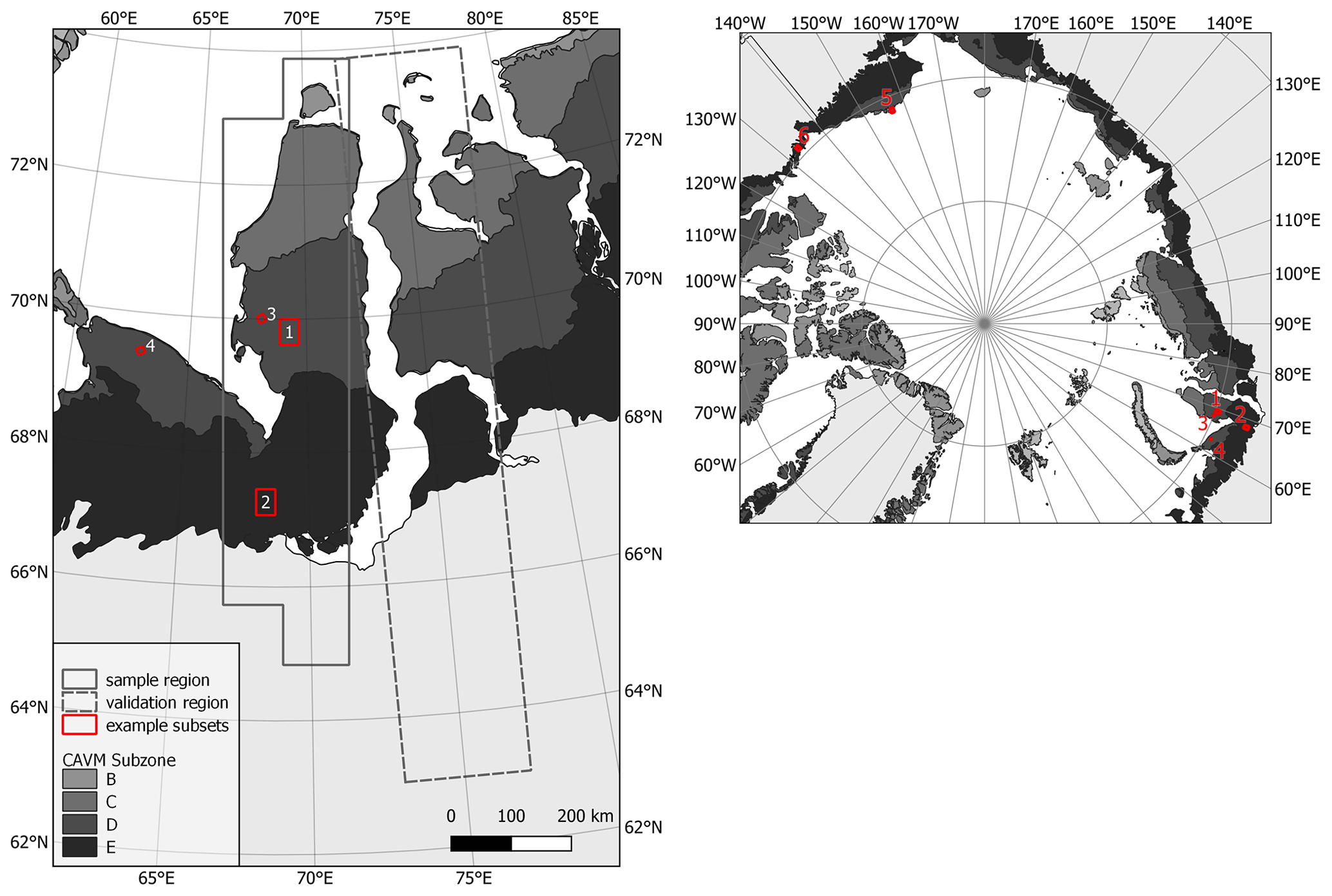
Figure 1 Location of subsets discussed in the study. Left: the training region for the maximum likelihood approach used for transfer to the circumpolar domain based on the prototype (k-means analyses; “sample region”) and the evaluation region (“validation region”). Right: sites of examples of the results presented in Fig. 14 (subset 1), Fig. 15 (subset 2), Fig. 16 (subset 5), Fig. 17 (subset 6) and Fig. 19 (subsets 3 and 4). Example locations are shown in both maps. CAVM – Circumpolar Arctic Vegetation Map (Raynolds et al., 2019) with subzones B, Arctic tundra, northern variant; C, Arctic tundra southern variant; D, northern hypo-Arctic tundra; and E, southern hypo-Arctic tundra.

2.3 In situ data

Three types of in situ records were available: (1) full pedon descriptions for key regions, (2) field data of soil surface organic horizon depth available from multiple sites across the Northern Hemisphere, (3) vegetation coverage records from the Russian Arctic Vegetation Archive for West Siberia (over view map in Fig. A1). More than 3500 in situ data records were used.

The field soil sampling took place between 2006 and 2019 and produced 355 pedons available for this analysis. Protocols for field sampling, laboratory analyses and data are detailed in Palmtag et al. (2022). Surface organic horizon depth was available for 788 non-forest samples, extracted from several different sources, including Hugelius et al. (2013, 2014, 2020) and Palmtag et al. (2022). Soil horizons were defined as organic when their organic carbon content was ≥ 17 % (equivalent to ca. 30 % organic matter content; Hugelius et al., 2020).

We used the information from the Russian Arctic Vegetation Archive (AVA standardized protocol, Zemlianskii et al., 2023), which contains relevés (geobotanical plots) made in accordance with the Braun-Blanquet tradition (available for download on the AVA website at https://avarus.space, last access: 6 March 2023). The relevés include species lists and species' cover estimations, as well as vegetation and habitat characteristics. They cover square plots with an area of 1–400 m² (74 % cover 100 m², 12 % cover 4 m² and other variants comprise less than 10 %). These plots were typically distributed across a 10×10 km site to ensure the representation of various plant communities with a statistically significant number of plots. The AVA data used in this study were obtained during fieldwork conducted from 2007 to 2020. A total of 2705 relevé locations overlapped the analysis extent (area within CAVM boundary).

The following in situ measurements are used for the assessment and assignment of unit descriptions.

1. Sites with full pedon descriptions are used (Palmtag et al., 2022), including the following:

   • volumetric water content (%),

   • organic volumetric content (%),

   • mineral volumetric content (%),

   • wet and dry bulk density, and

   • soil organic carbon and total nitrogen density.

2. Sites with soil surface organic horizon depth (cm) (partial overlap with (1)) are used.

3. Vegetation coverage (%) is used (from AVA; https://avarus.space/profile/about/, last access: 6 March 2023, Zemlianskii et al., 2023), including the following:

   • trees,

   • tall shrubs,

   • low shrubs,

   • erect dwarf shrubs,

   • prostrate dwarf shrub,

   • graminoids,

   • tussock graminoids,

   • forbs,

   • seedless vascular plants,

   • mosses and liverworts,

   • lichen,

   • crust,

   • algae,

   • bare soil,

   • bare rock, and

   • litter.

The AVA dataset (3) also includes a general wetness description (dry, moist, wet and aquatic) and open-water fraction.

2.4 Auxiliary data

The analysis extent also includes disturbances, specifically wildfire-affected areas within the tundra-taiga transition zone, which need to be considered in the assessment. The Alaska Large Fire Database (https://www.frames.gov/catalog/10465, last access: 28 September 2023) contains current and historical reported fire locations and fire perimeters. It builds on Kasischke et al. (2002). The database covers all of Alaska and contains about 4600 polygons for fire extent dating back to breakouts in 1942. Polygons which overlap with the analyses extend back to 2002. The latest fires represented are from October 2021.

Digital elevation data are required for pre- and post-processing of the satellite data. The Copernicus DEM GLO 90 was used. It represents the surface of the Earth including buildings, infrastructure and vegetation at 90 m spatial resolution. It covers the full global landmass of the time frame of data acquisition (2011–2015). The Copernicus DEM is based on the SAR-derived WorldDEM dataset provided by Airbus and acquired by the TanDEM-X mission. According to official statistics published by Copernicus in the DEM Product Handbook, the overall absolute vertical accuracy of the dataset is 90 %, and the confidence level is > 4 m. For Svalbard, the 20 m spatial resolution DEM of the Norwegian Polar Institute was used (Melvaer, 2014). This DEM is based on stereo models of aerial photos.

Air temperature was derived from ERA5 reanalysis data which combine model data with observations to provide a globally consistent dataset (Hersbach et al., 2023). The data were available from the European Centre for Medium-Range Weather Forecasts (ECMWF) and accessed via the Climate Data Store (CDS). We used air temperature at 2 m above the surface in a temporal resolution of 2 h at 0.25° spatial resolution for selection of Sentinel-1 observations. Precipitation was used in addition in order to clarify anomalous weather conditions (drought and flooding conditions) impacting the results in the final maps.

2.5 Existing land cover information for comparison

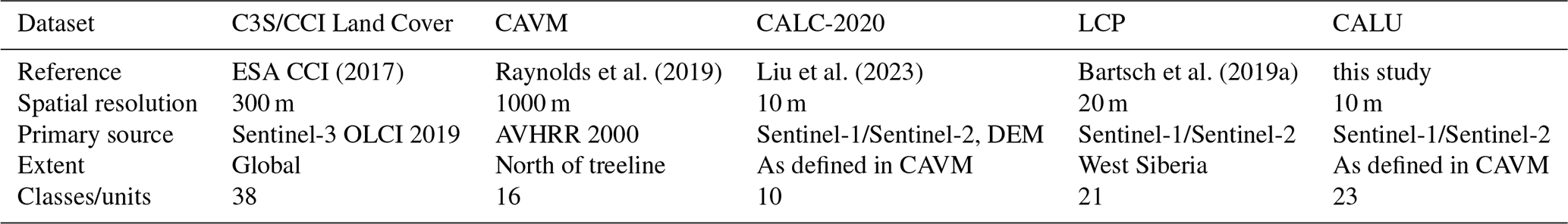
Two circumpolar and one global land cover dataset were compared to the land cover units (Table 1). The spatial resolution ranges from 10 to 1000 m. The raster version of the CAVM (Circumpolar Arctic Vegetation Map; Raynolds et al. (2019)) is considered a key benchmark dataset as it was developed specifically for the Arctic by vegetation experts. It provides a similar level of detail as anticipated in this study regarding shrub types and soil wetness.

Raynolds et al. (2019)Liu et al. (2023)Bartsch et al. (2019a)

Table 1 Land cover datasets considered for cross-comparison. CCI – ESA Land Cover Climate Change Initiative (CCI) (2017) project (http://maps.elie.ucl.ac.be/CCI/viewer/index.php, last access: 1 September 2023). CAVM – Circumpolar Arctic Vegetation Map. CALC-2020 – Circumpolar Arctic land cover. LCP – land cover prototype. CALU – Circumarctic Land cover Units.

The CAVM also includes information on bioclimatic subzones. In total, five subzones are distinguished for the Arctic, of which four can be found along the validation and calibration region (Fig. 1).

3 Methods

In a first step, a land cover unit retrieval scheme was adapted in order to achieve 10 m nominal resolution; consider atmospheric correction; address issues in mountainous regions; and allow additional classes such as recent fire scars, snow and shadow. Results were cross-compared to results of the original processing scheme and to external datasets including classical land cover maps and soil and vegetation in situ records. The latter were used to provide an example for description of the units.

Statistics were derived for 1 km × 1 km areas in a second step in order to quantify land cover diversity in general and specifically for wetland areas.

3.1 Land cover units retrieval scheme adaption

The retrieval scheme expands the prototype (Bartsch et al., 2019b) from West Siberia to the entire Arctic, incorporating advanced pre-processing, and a postprocessing step was introduced. The final classes are referred to as land cover units and the map as a whole as CALU – Circumarctic Land cover Units. The prototype is based on an unsupervised k-means classification. The resulting classes are units of similar reflectance of the shortwave incoming radiation (Sentinel-2) and radar backscatter at C-VV (Sentinel-1). Names for the prototype units were assigned by regional experts to the 23 resulting classes.

The processing was based on Sentinel-2 granules as defined by the data provider. Granules have an extent of 100 km by 100 km. They partially overlap as they are aligned with respect to UTM projection zones. Only granules including ice free land areas were considered. All Sentinel-1 images were subset to the granules.

Sentinel-2 data are available in UTM projection and largely at Level 2A (orthorectified, top of atmosphere). Atmospheric correction was required in order to account for related differences between the dates. We therefore applied atmospheric correction using sen2cor on the Sentinel-2 data (Main-Knorn et al., 2017), which also generated a cloud mask during the process. Sentinel-2 provides spatial resolution of 10 m for some bands but not for all. Enhancement of spatial resolution of the coarser band therefore needed to be considered to exploit the multispectral capabilities offered by Sentinel-2. We therefore performed super-resolution based on the tool Dsen2 (Lanaras et al., 2018), which used a convolutional neural network. Lanaras et al. (2018) showed that their approach clearly outperformed simpler upsampling methods and better preserved spectral characteristics. The original model was trained on Level-1 data, which were not atmospherically corrected, and global sampling. Bartsch et al. (2021a) retrained and tested the model on Level-2 data (output of sen2cor) using the same published training and testing routines for selected granules from our study sites. After the super-resolution step, clouds were masked using the cloud mask output from sen2cor. In the case of frequent fractional cloud cover, subsets of scenes were also used. Mostly, mid-growing season acquisitions were considered for Sentinel-2; this means mid-July to mid-August. This time frame was slightly extended in some cases with limited cloud-free acquisitions. Up to eight Sentinel-2 acquisition dates were selected for individual granule locations. A minimum of three were collected if available. In a next step, the median of the acquisition dates was calculated, which further mitigated errors due to undetected clouds.

Acquisitions needed to represent frozen conditions in the case of Sentinel-1 but at a maximum of −10 °C to minimize the effect of temperature on backscatter at C-band (Bergstedt et al., 2018; Bartsch et al., 2023a). This required the use of spatially consistent temperature data across all analysed areas. Reanalysis data (ERA5) were therefore used for scene selection. Processing steps of Sentinel-1 included border noise removal, based on the bidirectional all-samples method of Ali et al. (2018), calibration, thermal noise removal and orthorectification using the Copernicus 90 m resolution DEM. These steps were carried out with the SNAP toolbox provided by ESA and γ⁰ was derived. After normalization, data were reprojected and subset to match the Sentinel-2 granules, and temporal averaging was performed.

A training area spanning 9° in latitude and representing different landscape gradients and thus all units (Fig. 1) was selected from the prototype land cover unit map in order to transfer the retrieval (retraining of the maximum likelihood classifier) to the entire Arctic as well as to the output of the enhanced pre-processing (super-resolution processing, atmosphere correction and use of γ⁰ instead of σ⁰). The units remained largely the same. Of the 21 original classes, 18 were assigned to the new units. The remaining 3 classes were modified and split up. First, the original mixed and coniferous forest units were both split regionally (bioclimatic zone E versus B to D) to address misclassification of tundra as forest. Pixels in zones B and D were joined and assigned to a new unit. The disturbance unit originally combined different disturbance types, which led to vegetation removal, geomorphological processes and fires. A k-means classification was applied to target two units. Results were preliminarily assessed with data from recently burned areas within the prototype extent in Western Siberia. The new “recently burned” unit was then validated over Alaska. The originally three water units were merged into one water unit. The modified prototype classification was then used to train the maximum likelihood classifier. Further on, a snow and a shadow unit were introduced based on training data from Svalbard, resulting in 23 units.

Illumination conditions impact the reflectance in the Sentinel-2 bands in mountainous areas. Not all shadow areas could be identified, due to similarities in reflectance with water bodies and wetlands. Therefore a second post-processing step based on the slope derived from the Copernicus DEM data was introduced. “Water”, “permanent wetlands” or “shallow water” on slopes larger than 7° were set to “other”. Shadow in regions with low slope (less than 3°) was set to “water”.

3.2 Evaluation and documentation of land cover units

Unit-specific validation was carried out for the new disturbance unit which targets burned areas using the Alaska Fire Database. The description of the units was based on the comprehensive soil and a vegetation in situ dataset. The first was previously used similarly in conjunction with a global land cover map (Palmtag et al., 2022). The second dataset is part of a tundra-specific international standardization and archive effort (Zemlianskii et al., 2023). Common statistics (mean, standard deviation) were derived and are supplied with the dataset documentation.

Unit descriptions consider abundance of vegetation types including shrub growth form/height as well as moisture conditions. The following shrub types were considered (following the differentiation of the CAVM; Raynolds et al. (2019) and Walker et al. (2018)):

• prostrate dwarf shrub – approximately 5 cm, also referred to as prostrate shrub;

• erect dwarf shrub – up to 40 cm, also referred to as dwarf shrub

• low shrub – up to 2 m;

• tall shrubs – tundra biome species taller than 2 m.

The comparison to CCI Land Cover and the CAVM (see Table 4) required resampling. The coarser-resolution maps were resampled to 10 m (the same resolution as CALU). Classes were grouped for comparison due to the large differences in thematic content. A simplified set of nine units was developed that allowed cross-comparison between the CALU and the three external maps. Table 2 shows the grouping for the CALU, and Appendix C shows the groupings for the external maps. In addition, the new classification was compared with the original prototype (20 m, 21 classes). A different training area was used for the evaluation than for the retraining of the transfer samples (Fig. 1).

Table 2 Example of representation of the Circumarctic Land cover Units (CALU) based on in situ records (see Fig. A1) and grouping (A) for comparison with other land cover maps and (B) for wetness heterogeneity assessment. In addition, the proportion within the CAVM (Circumpolar Arctic Vegetation Map; Raynolds et al. (2019)) extent is provided in percent (P) and the majority proportion (1 km grid cells) in percent (M). ^* Sparse tree cover along treeline. nd: no data.

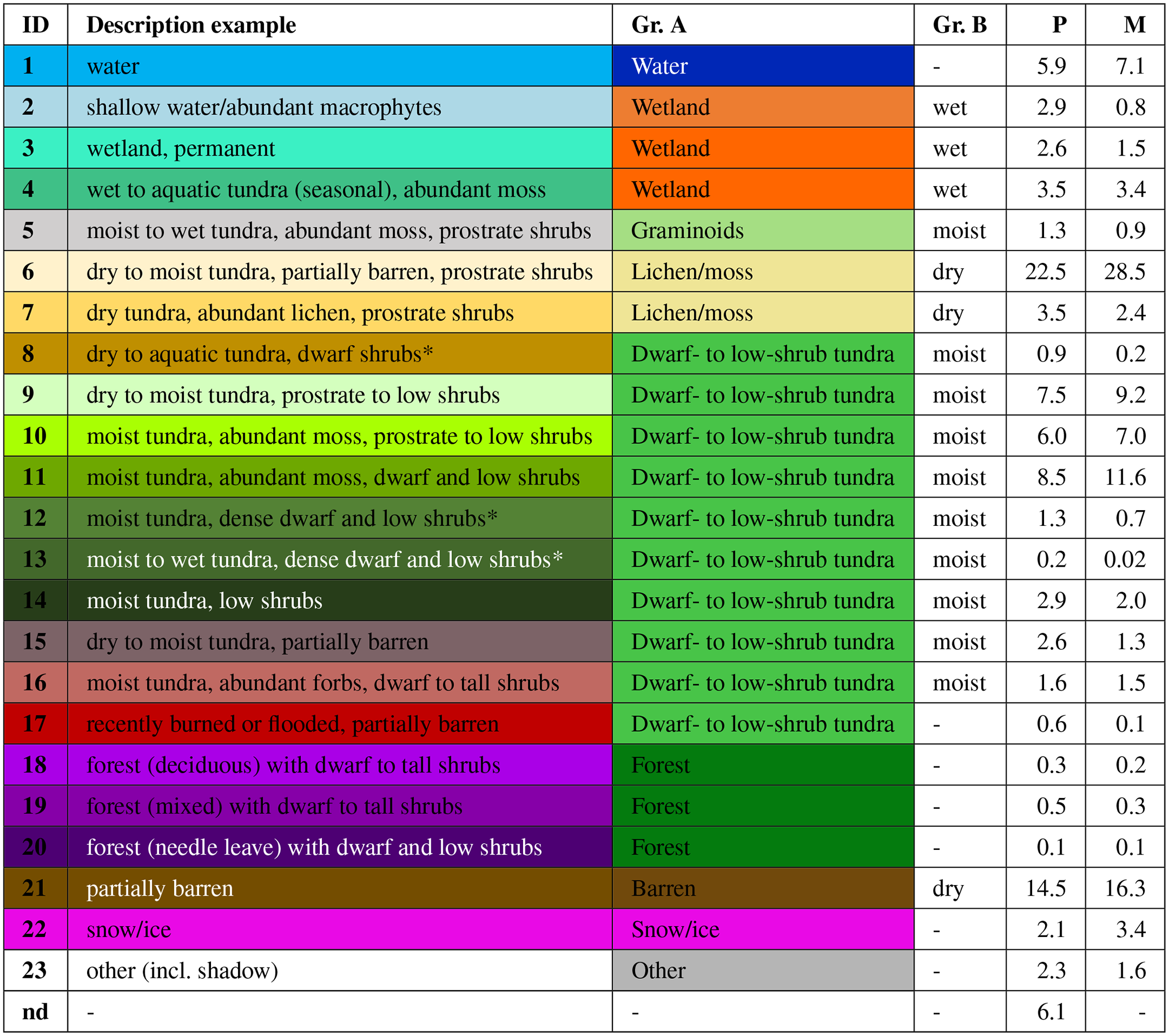
A direct comparison could only be made for common or merged classes, which included water, snow/ice, other, wetland, graminoids, lichen/moss, dwarf- to low-shrub tundra, forest and barren (without graminoids). The grouping of CALU for the comparison was primarily guided by the presence of shrubs. If more than 20 % of erect dwarf to low shrubs were found on average, the unit was assigned to shrub tundra. The assignment is referred to as grouping A (Table 2).

3.3 Heterogeneity assessment

Landscape heterogeneity was addressed through assessment of (1) richness with respect to the CAVM classification specifications and (2) wetness diversity, both for 1 km grid cells. The chosen cell size matches the grid of the permafrost model CryoGRID (Obu et al., 2021) as well as the raster version of the CAVM (Raynolds et al., 2019). The number of identified units (minimum 1 % fraction) within 1 km × 1 km cells was counted for the CAVM classes. Permanent snow and shadow were excluded from the richness assessment. In addition, units were grouped with respect to wetness (wet, moist, dry) for wetland and tundra classes, also excluding permanent snow and shadow as well as water, forest and recently burned areas. Groups (referred to as B, Table 2) were summed up, resulting in values of 1 (homogeneous) to 3 (heterogeneous).

4 Results

4.1 Coverage

In total, 1266 Sentinel-2 granules which overlap with the Arctic as identified in the CAVM (Raynolds et al., 2019) were identified (Fig. 2). The use of three Sentinel-2 acquisitions was targeted to account for anomalies due to undetected clouds and hydrological extremes (droughts, flooding), which was achieved in 75 % of the cases (Fig. 3). Only two images were available for 4 % of all granules. More than 3600 Sentinel-2 images at granule extent were included in the processing.

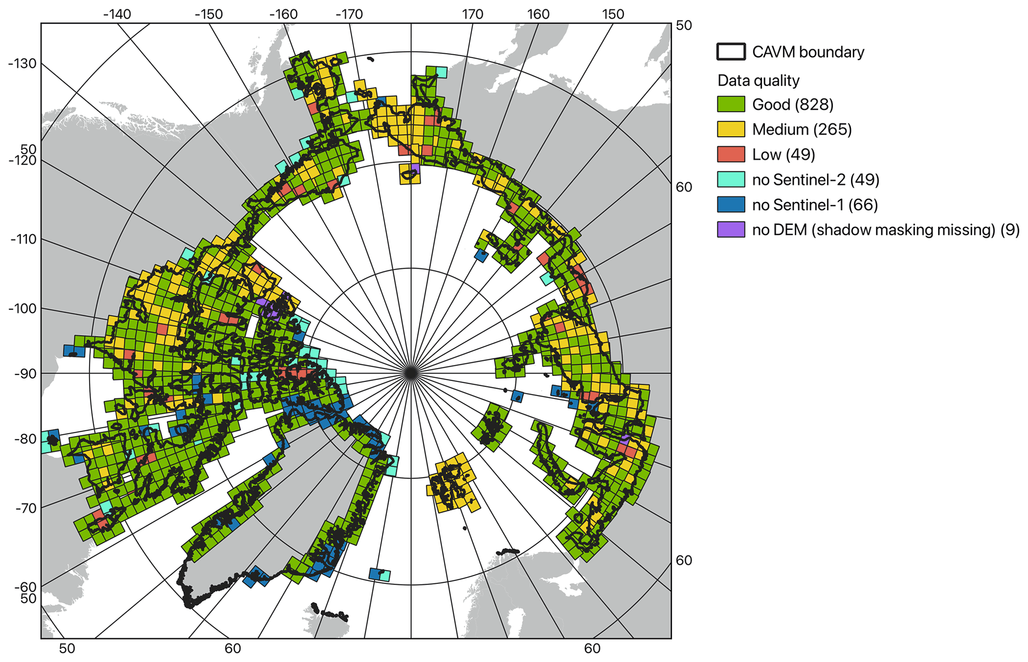
Figure 2 Data quality by granules within the Circumpolar Arctic Vegetation Map (Raynolds et al., 2019) boundary, with the number of granules in parentheses.

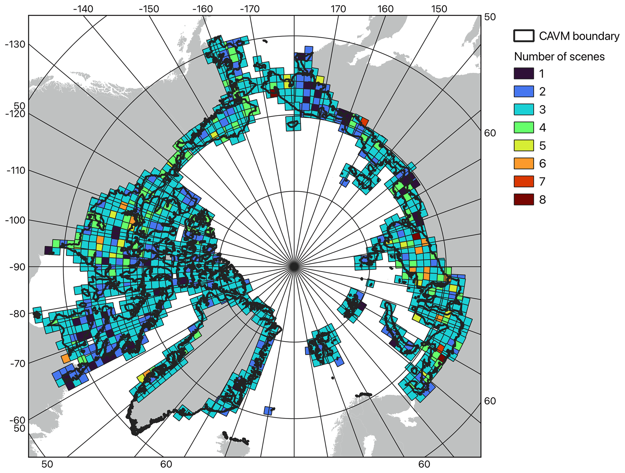
Figure 3 Number of Sentinel-2 scenes used, by Sentinel granule, within the Circumpolar Arctic Vegetation Map (Raynolds et al., 2019) boundary.

No suitable Sentinel-2 acquisitions were available in 49 (4 %) cases and, in addition, 66 (5 %) cases with no Sentinel-1 data (Fig. 2). The latter is related to the general Sentinel-1 acquisition strategy for IW mode. Data were missing specifically for Greenland and the Canadian High Arctic islands. Nevertheless, 97 % of the target area (CAVM extent) could be processed. In 13 % of the area, the availability of data was very limited and led to lower-quality results or gaps (Figs. 2 and 3). This results from acquisition date issues or inconsistencies in the Copernicus DEM (no data: 23 times in the case of some inland water bodies and 2 times for general gaps). In total, 19 % were flagged as being medium quality and 3 % as being low quality. Medium quality usually resulted from anomalous meteorological/hydrological conditions in certain years (evaluated with re-analyses), including flooding or droughts which impact land cover and vegetation optical properties. Low quality was usually caused by acquisitions close to mid-July and mid-August in years with deviations in phenology (early or late spring).

4.2 Identified land cover units

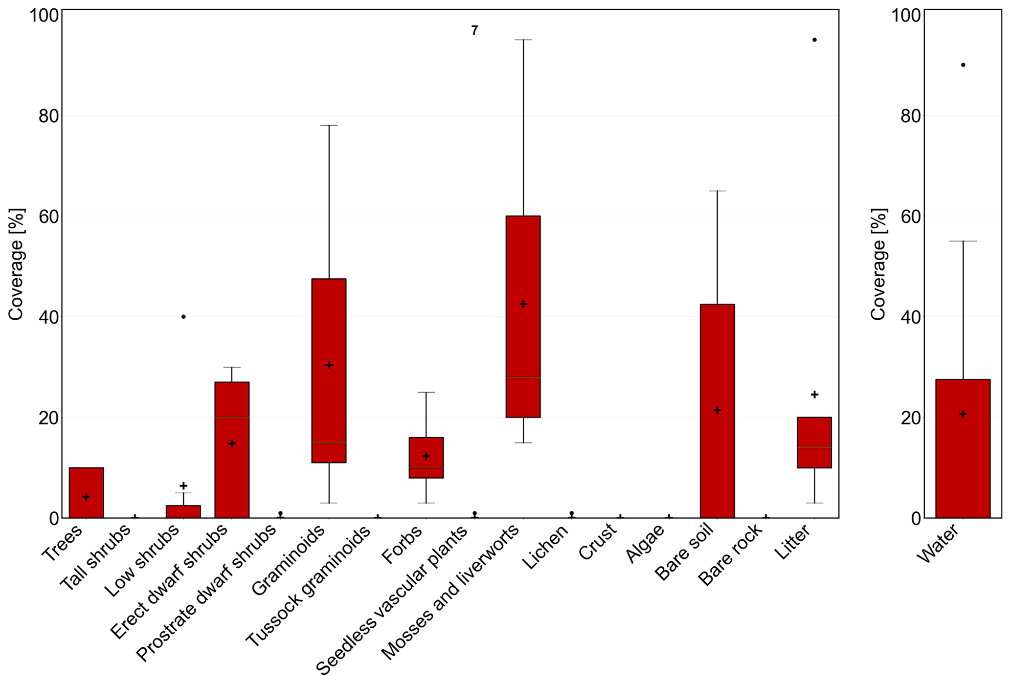
For the CALU (Circumarctic Land cover Units) map, 23 unit types were derived (Table 2). Descriptions were assigned summarizing the statistics of the in situ data, referring to wetness, vegetation physiognomy and abundance. The most common unit within the extent of the CAVM was unit no. 6 “dry to moist tundra, partially barren, prostrate shrubs” with overall 22.5 % (original 10×10 m) and 28.5 % in the majority (1×1 km) respectively. This unit could be specifically found in the Canadian High Arctic and on the Taimyr Peninsula (Russia). Units with shrubs of dwarf and higher growth form summed up to about 32 % and wetlands to about 9 %. A higher occurrence in the majority retrieval indicated relatively homogeneous patterns. This applied specifically to unit no. 6 as well as no. 21 (partially barren). The contrary was the case for wetland units no. 2 and no. 3, reflecting patchy occurrence at a scale of < 1 km². Regarding wetness, 40 % of the circumarctic area was assigned to the dry and 32 % to the moist group.

4.3 Characterization through in situ records

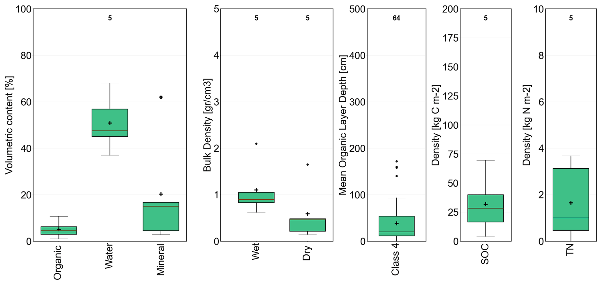
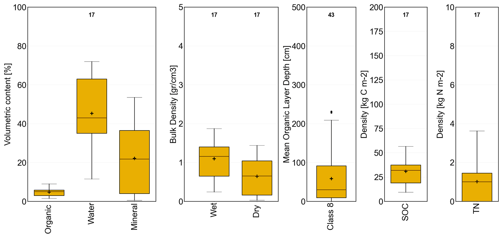
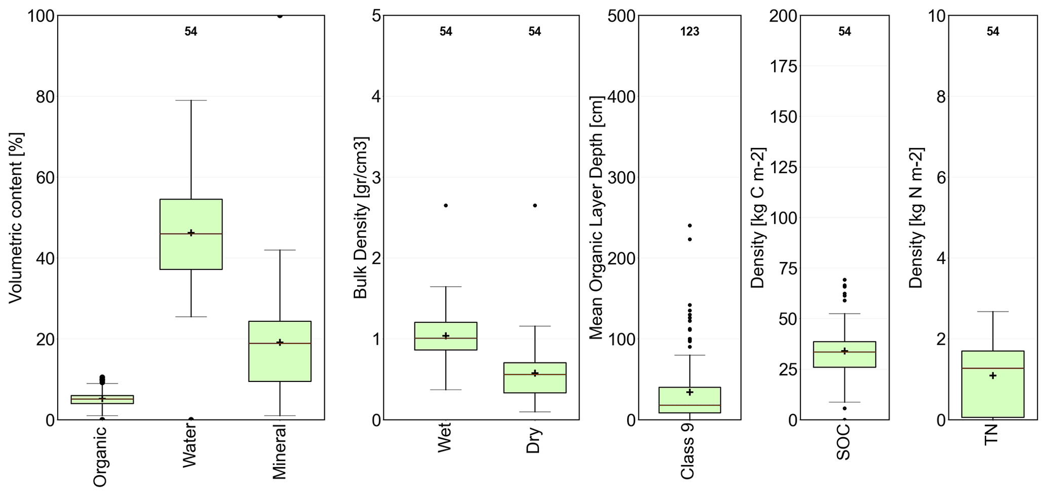
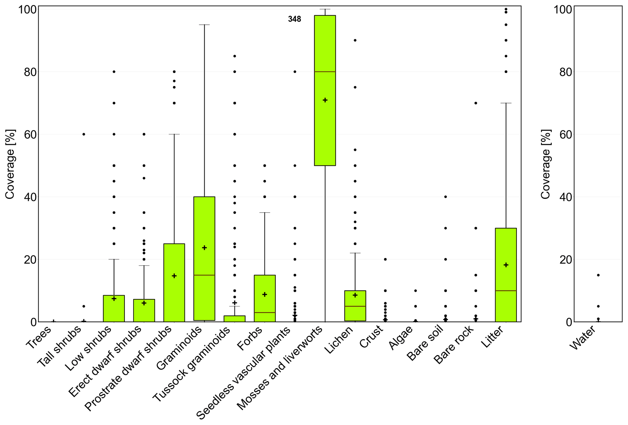
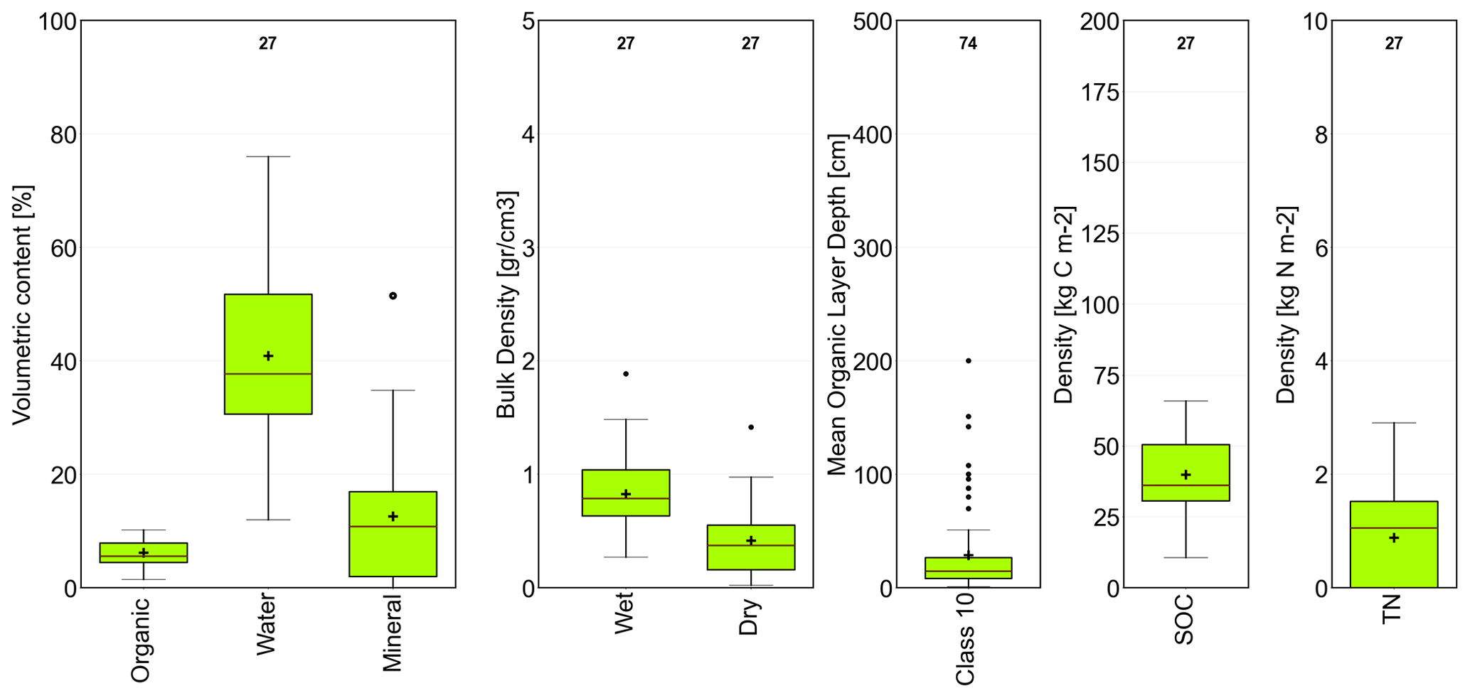
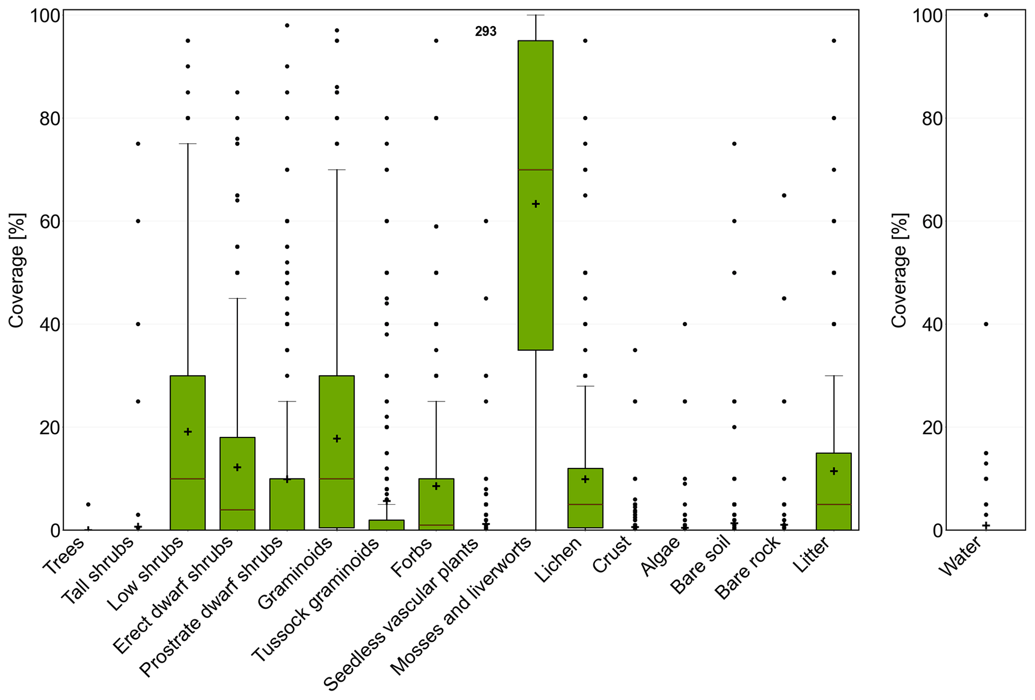
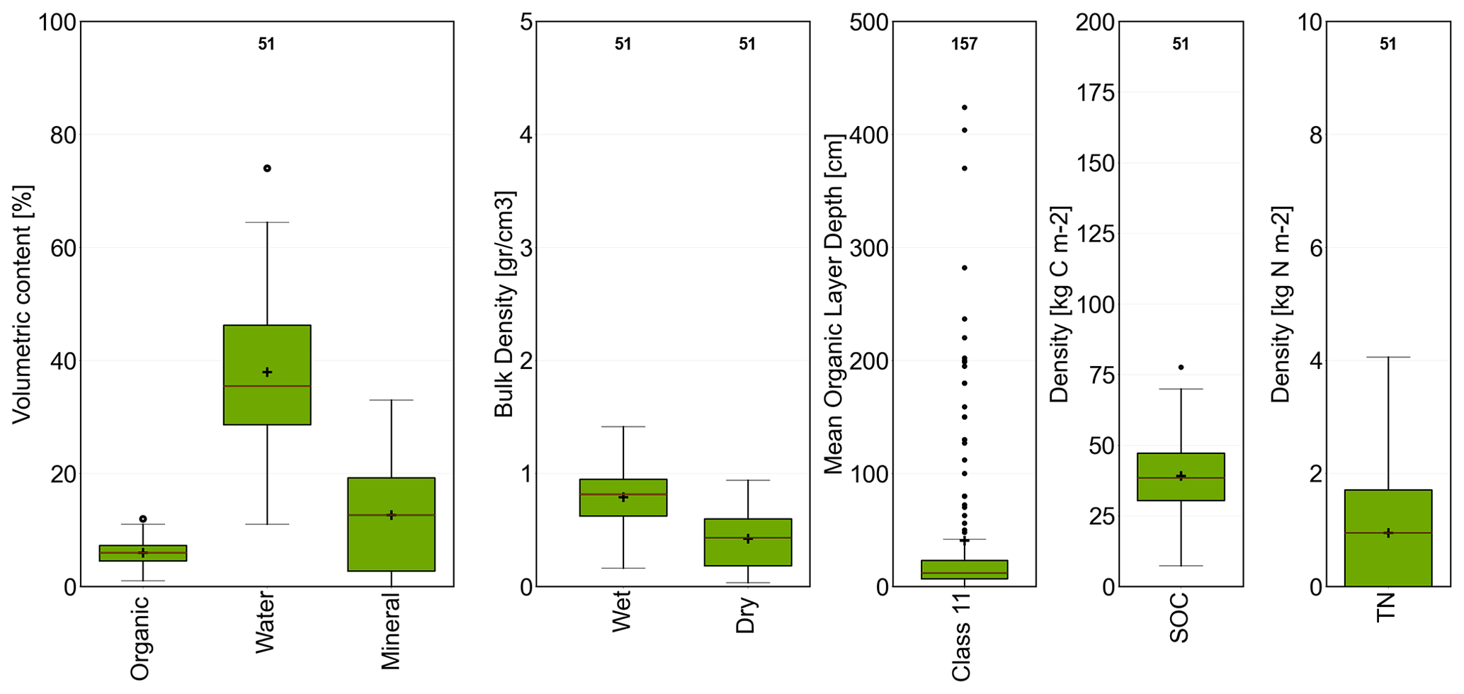
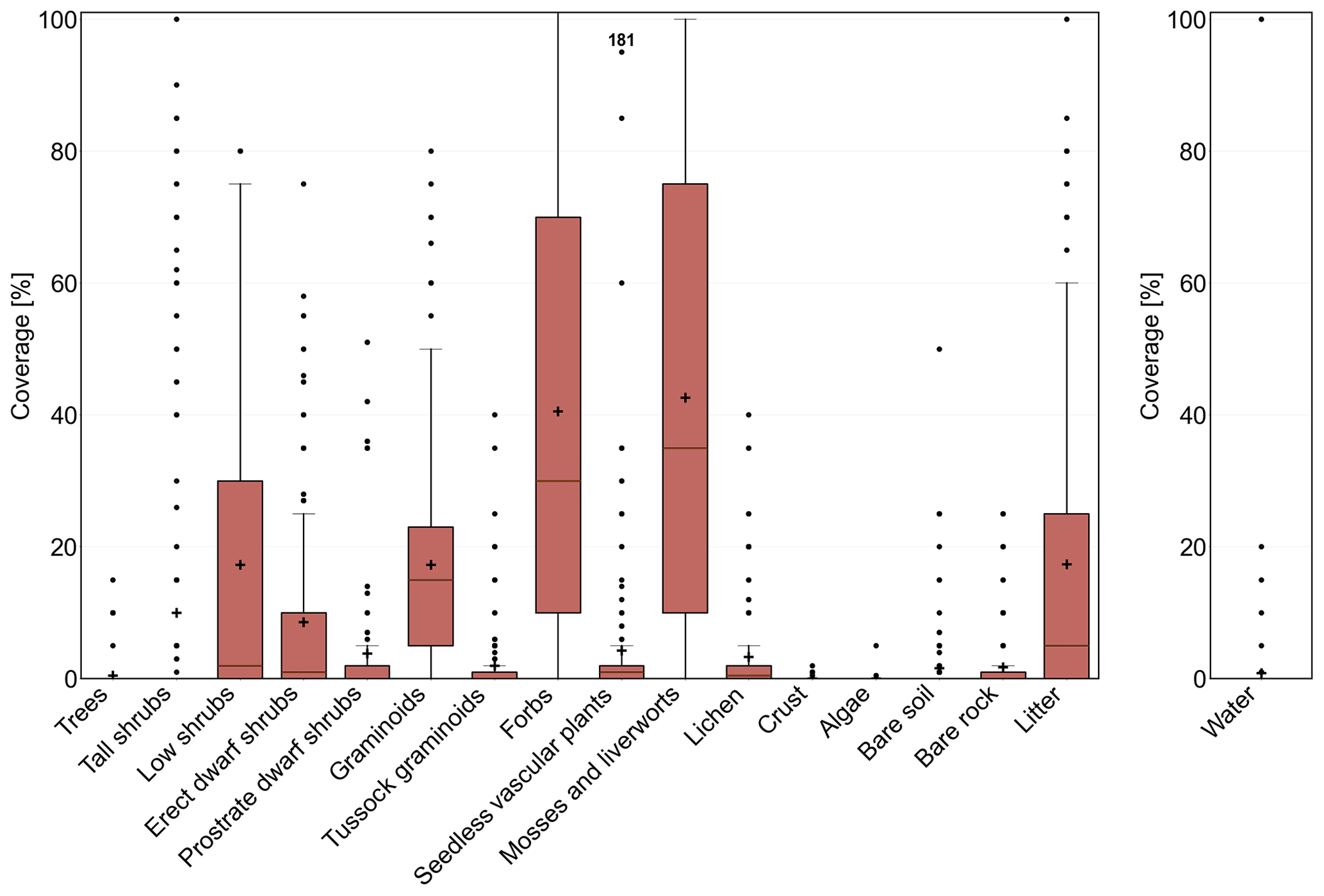
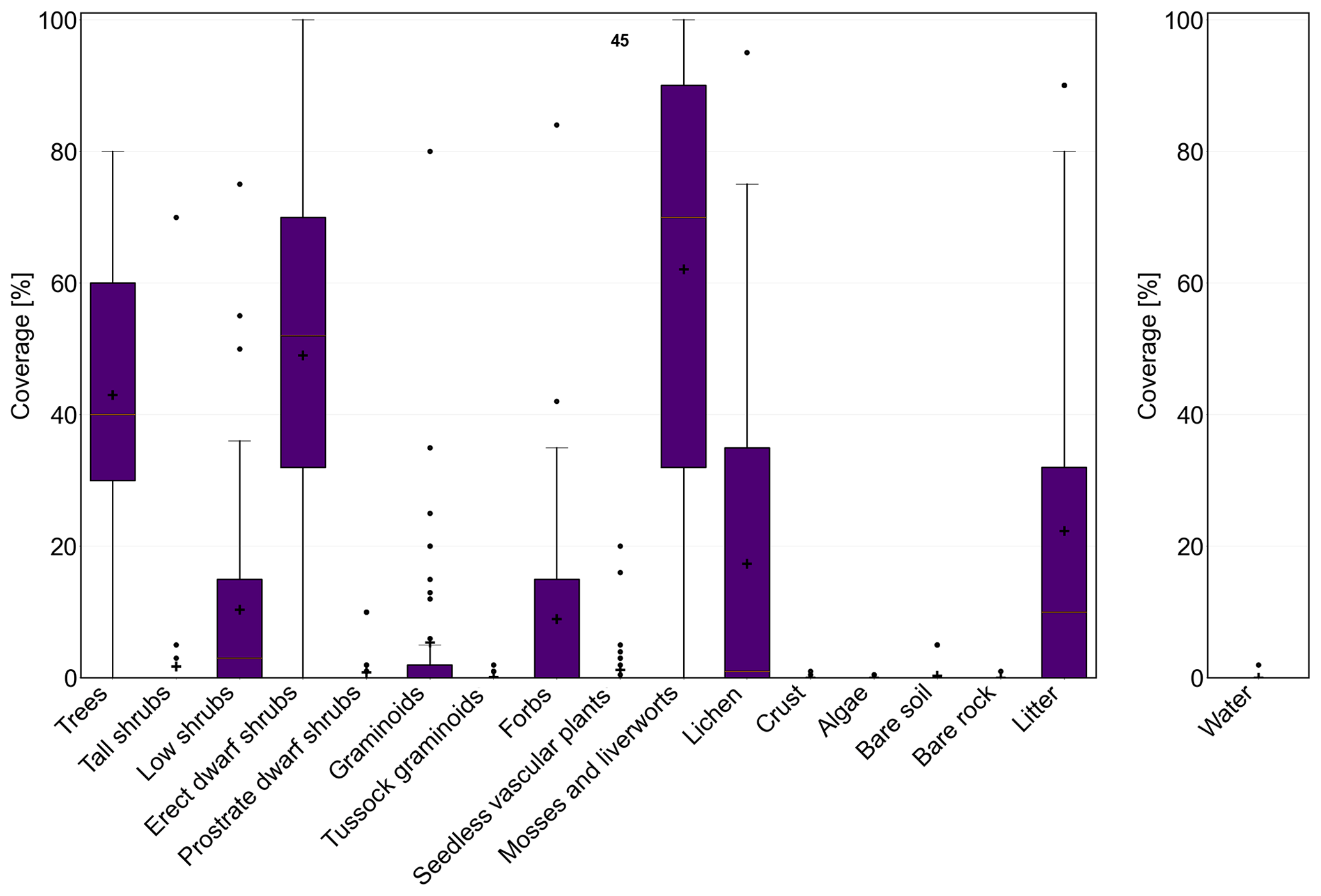
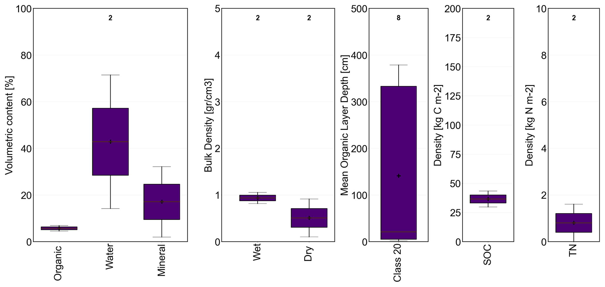
All units could be assigned vegetation compositions and water/mineral volumetric content (Table 3, Figs. 4, 5 and 6). There were differences in in situ data availability between the land cover units which needed to be considered. Soil data were largely unavailable for forest and disturbed sites (Tables A2, A1). The dry tundra unit, unit no. 7, which had the most abundant lichen coverage, had little pedon data but good vegetation description. Unit no. 13 lacked both pedon and vegetation description as it represents vegetation along incised creek channels (moist tundra, dense dwarf and low shrubs; Fig. B41) which were rarely sampled. Soil samples for inundated areas (unit no. 2) were unavailable. Vegetation samples for this unit are expected to be located at the boundary of shallow water bodies with macrophytes but in the same pixel. They were nevertheless included in the tables and figures. The lack of or very low number of samples of soil volumetric water content data for some units (no. 2 and no. 7) could be partially compensated for by general wetness information contained in the vegetation records (Fig. 6).

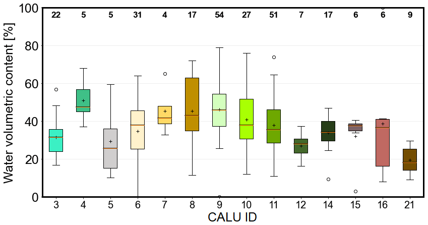
Figure 4 Volumetric water content statistics (box plot representing quartiles, median, mean as “+” and outliers as “°”) for Circumarctic Land cover Units (CALU) based on in situ data from Palmtag et al. (2022). Number of samples per unit are shown at the top. For unit details and colours, see Table 2.

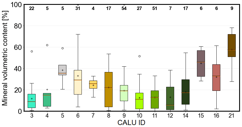
Figure 5 Mineral volumetric content statistics (box plot representing quartiles, median, mean as “+” and outliers as “°”) for Circumarctic Land cover Units (CALU) based on in situ data from Palmtag et al. (2022). Number of samples per unit are shown at the top. For unit details and colours, see Table 2.

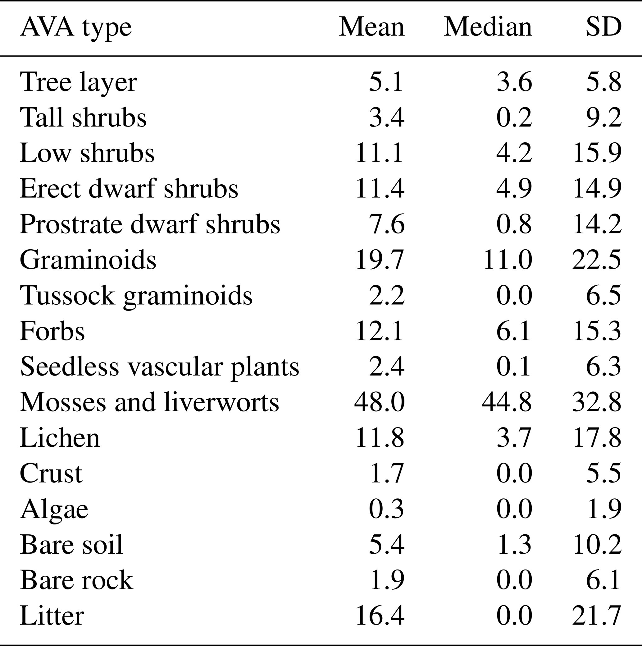
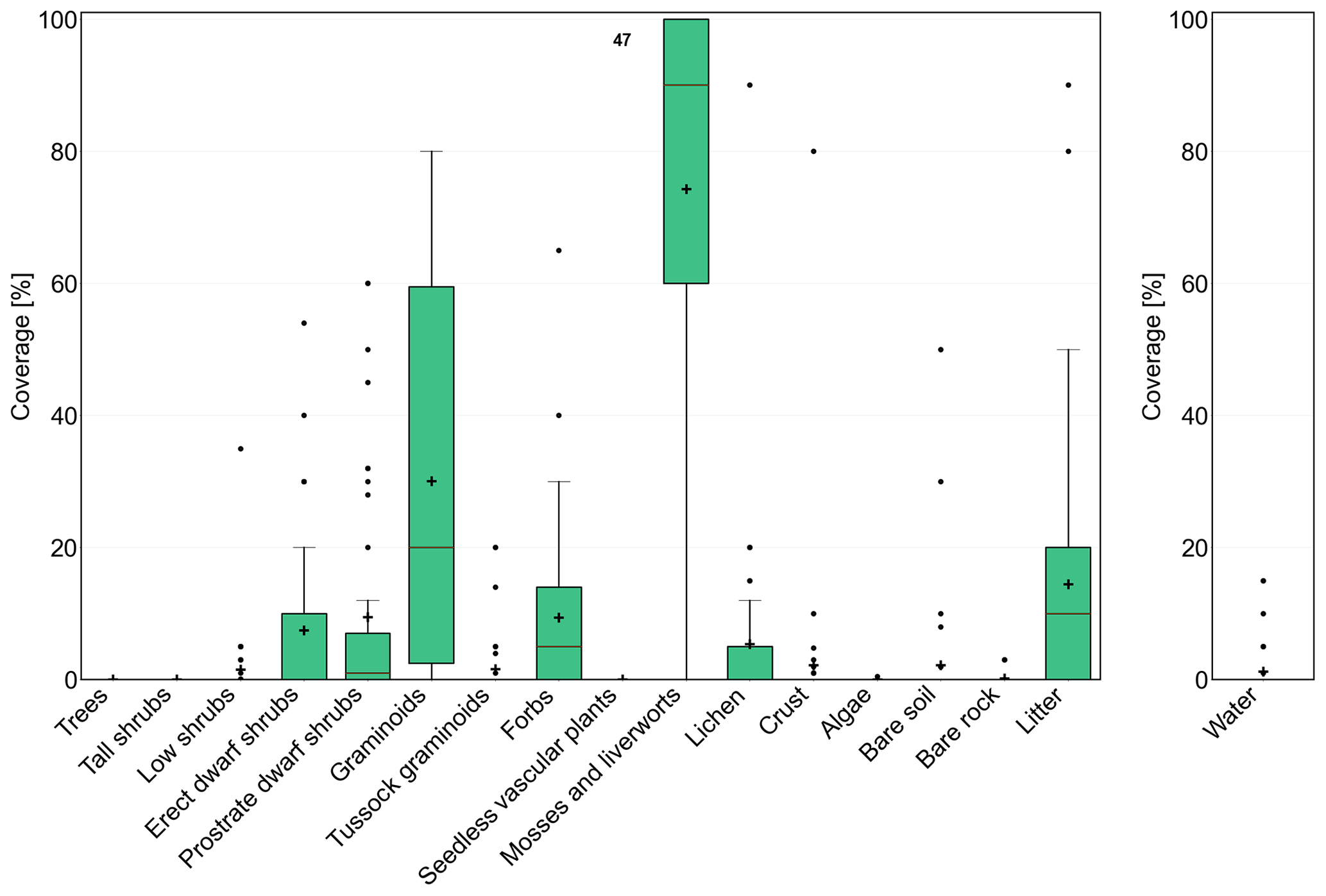
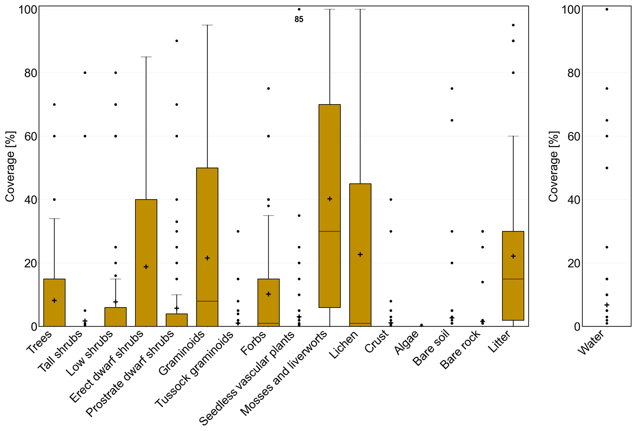
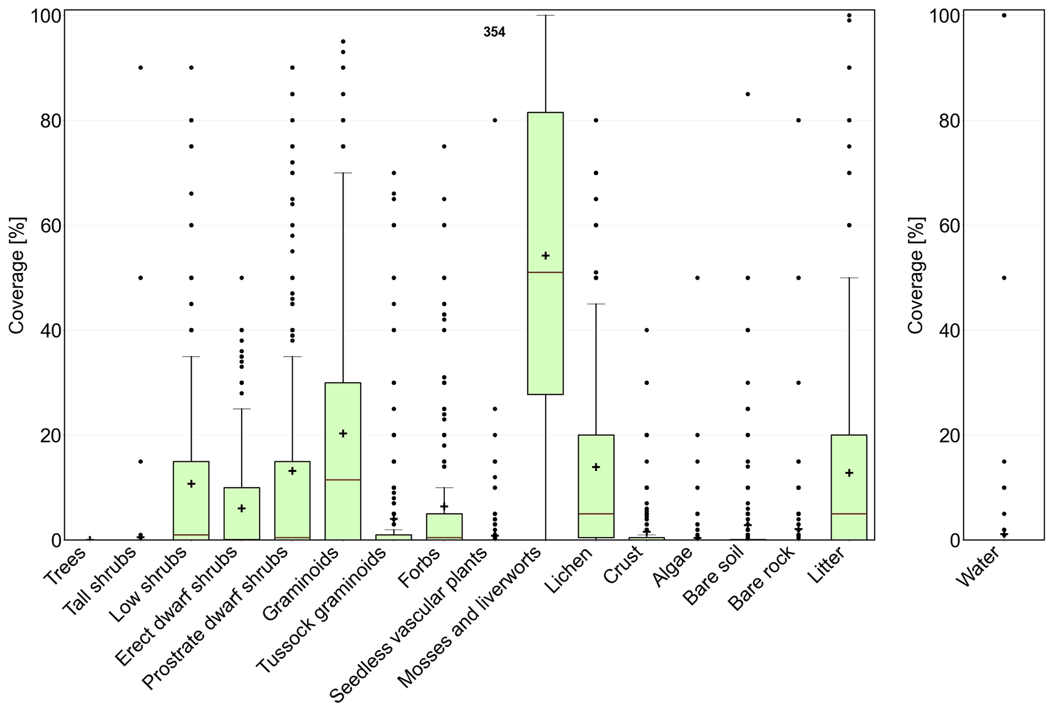
Table 3 Average coverage of different life forms for each Circumarctic Land cover Unit (CALU) based on Russian Arctic Vegetation Archive plots, West Siberia (Zemlianskii et al., 2023).

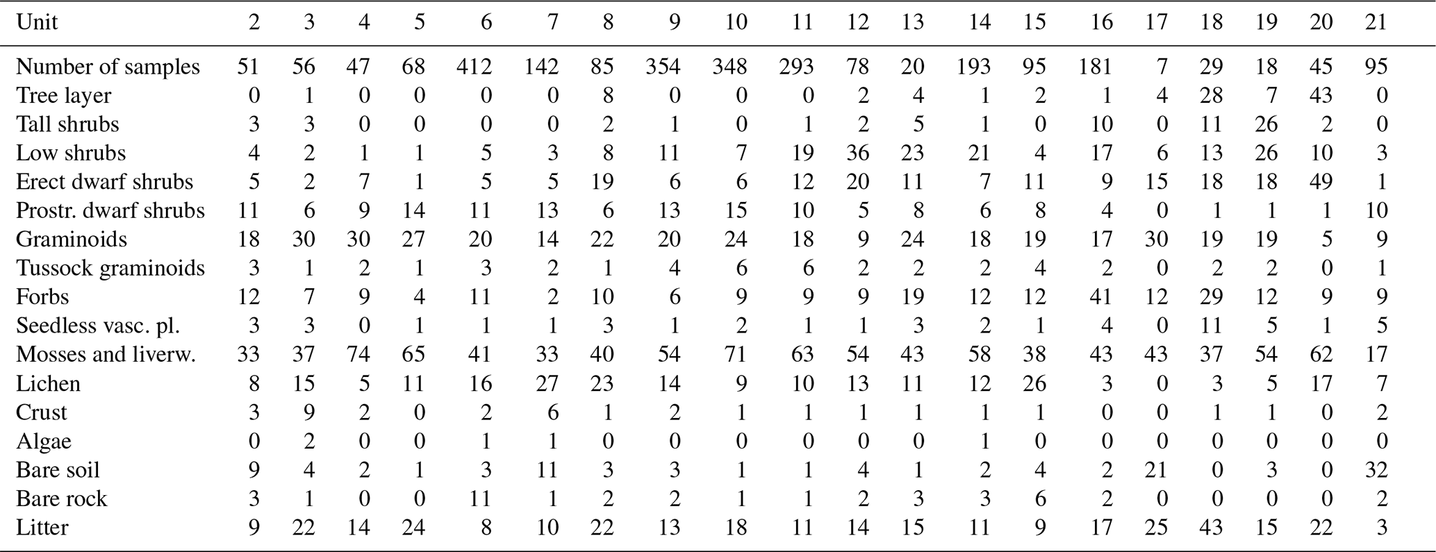
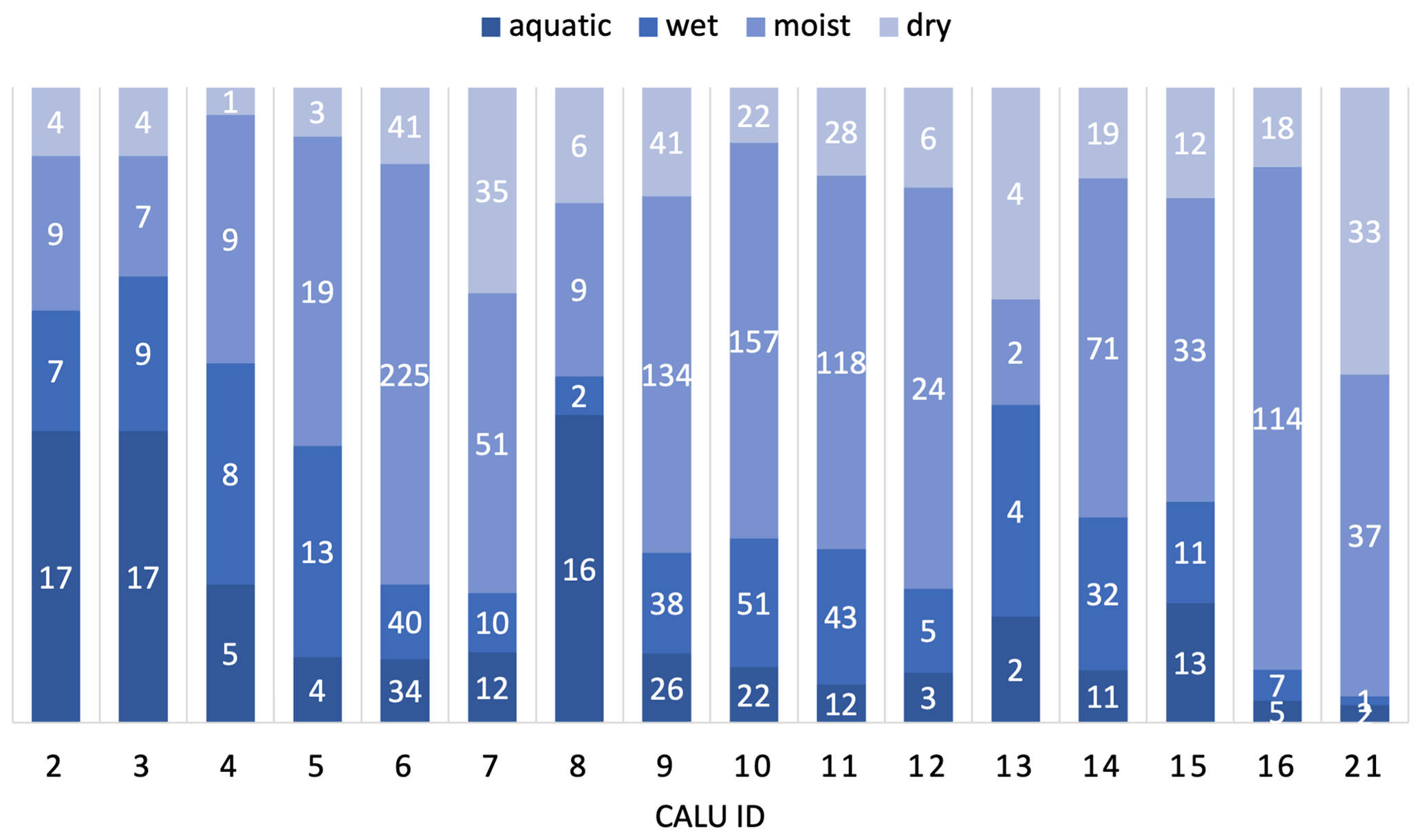
Figure 6 Wetness categories for Circumarctic Land cover Units (CALU) based on Arctic Vegetation Archive plots, West Siberia (Zemlianskii et al., 2023; units with at least 10 data points).

4.3.1 Vegetation

Mosses and graminoids were common across all units, with moss being most dominant (48 % overall average coverage) and graminoids the second most dominant (20 % overall average coverage) (Table 3). Lichens only had 12 % cover on average and only had over 20 % cover for units with comparably dry parts. Forbs were less abundant except for one case, unit no. 16, for which the average cover was 41 %. Mosses also showed the highest standard deviation within the land cover units (Table 3).

The “barren” unit, unit no. 21, had the highest bare ground fraction with, on average, 32 % for soil and 2 % for bare rock. Bare rock was most common in unit no. 6, with 11 % cover.

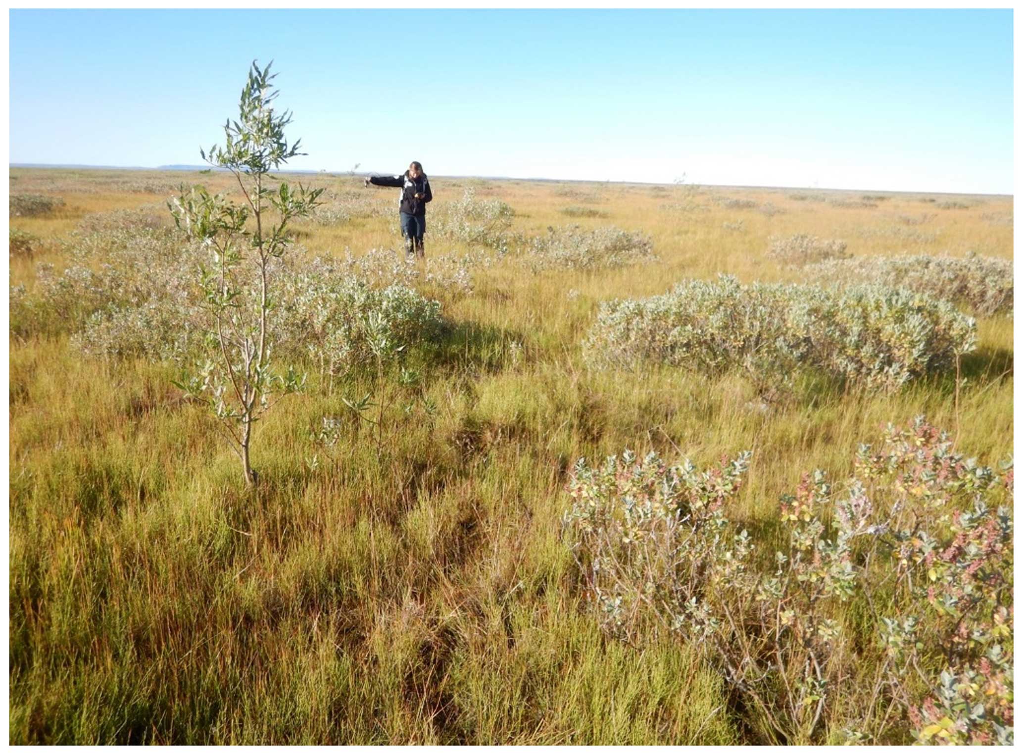
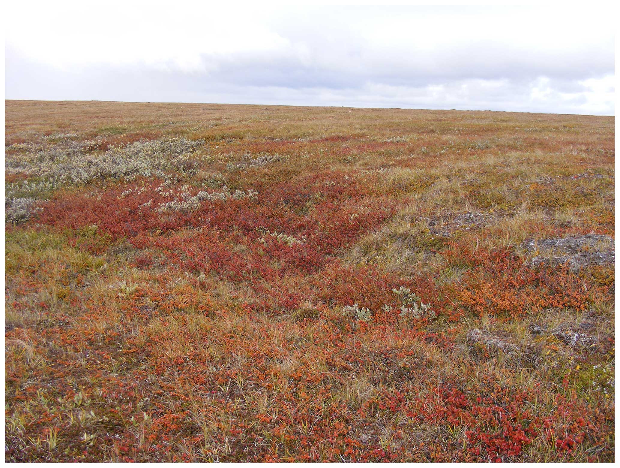
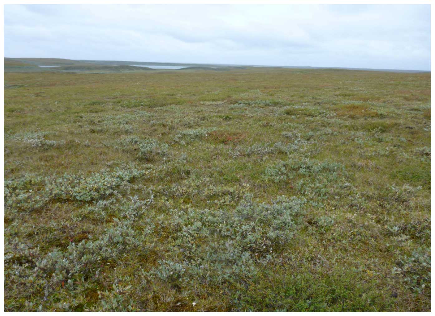
Unit no. 2 represents shallow water along lakes and seashores which are not well represented in the AVA or soil records (see example in Appendix Fig. B2). Vegetation and soil records (in the case of organic layer thickness) are taken on land along the lake margins. Presence of open water in the proximity is reported in the AVA records in some cases (Fig. B1). Macrophytes are abundant, emerging through the course of the summer season, as observed during alternative field surveys (see photograph in Fig. B3). The average open-water fraction in the AVA records is mostly close to zero (Appendix B) except for no. 2 (7.5 %), no. 3 (permanent wetland; 12%), no. 8 (dry to aquatic tundra; 7%) and no. 17 (recently burned area; 21%).

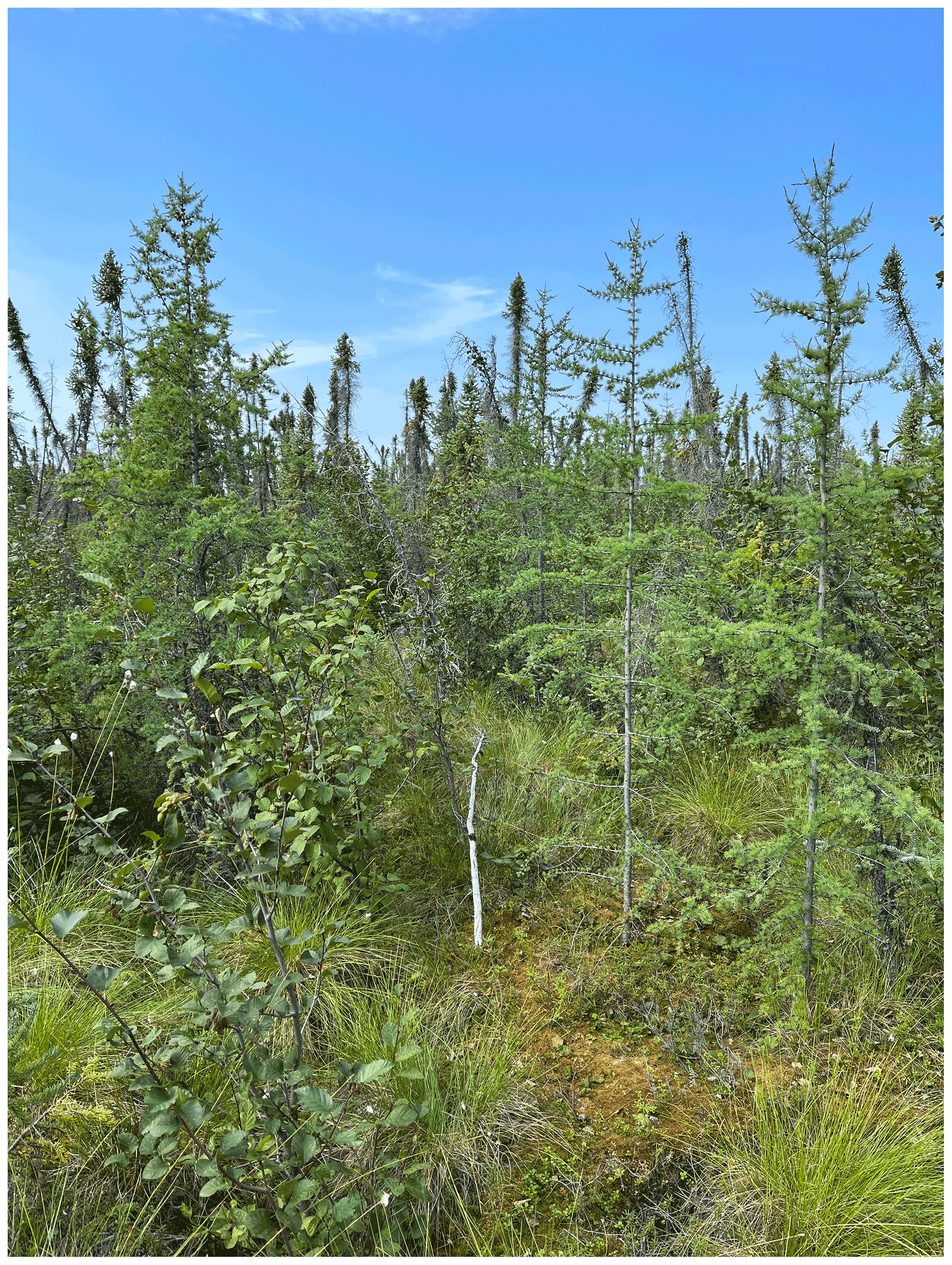
Several units with tall shrubs in proximity to the treeline also can include needle leaf trees (no. 8, no. 12 and no. 13; see Table 3). The latter are of limited height and also diameter due to the harsh environment and commonly occur in the North American treeline zone (Figs. B24 and B42). These areas correspond to the “woodlands” and “open stands” in definition level III according to Viereck et al. (1992) (10 % to 24 % crown canopy cover and 24 % to 60 % respectively).

4.3.2 Soils

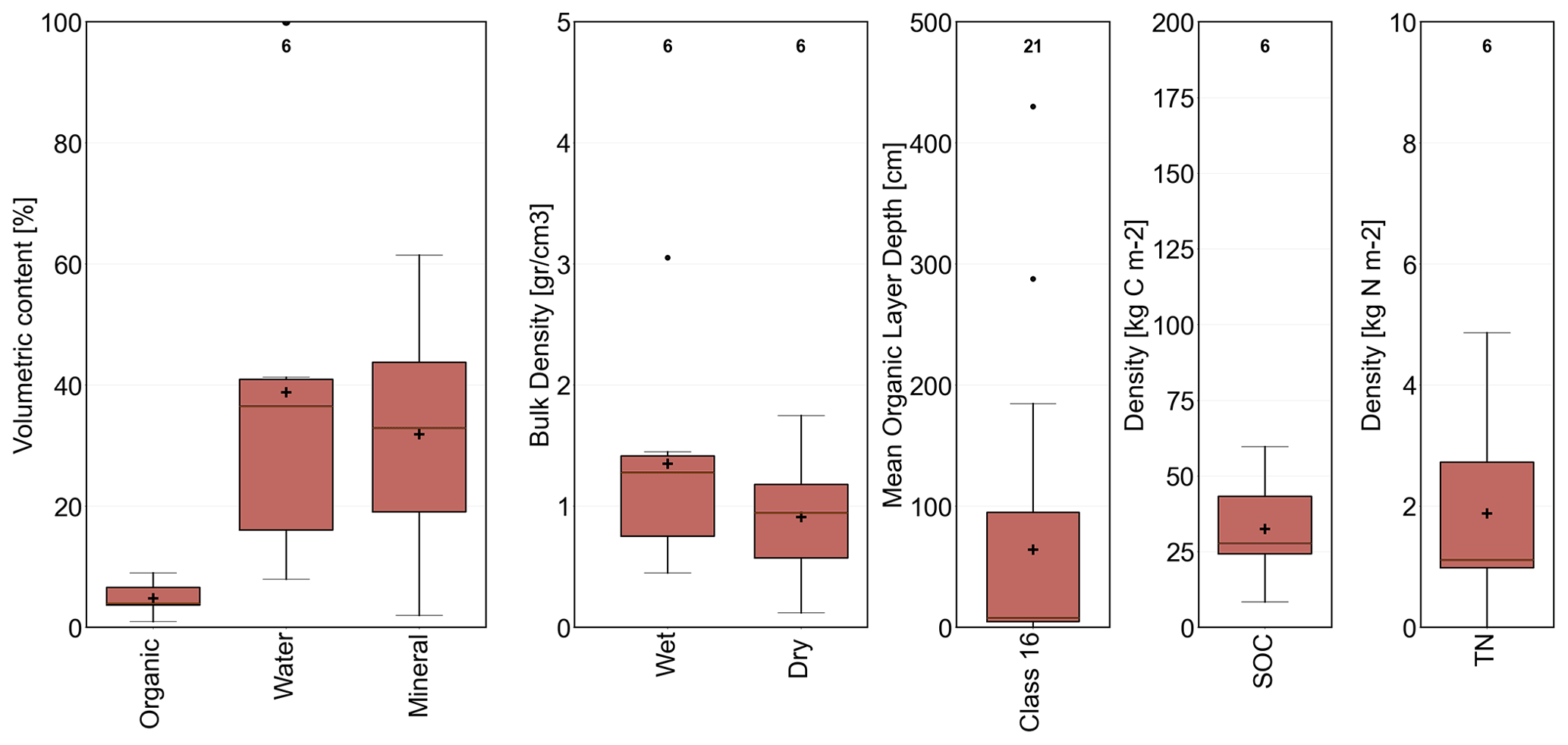
The units with a certain barren fraction (no. 6, no. 15 and no. 21; see Table 3) showed all comparably high mineral volumetric content (Table 3 and Fig. 5). Higher wetness (> 40 % volumetric content on average) could be found in permanent wetlands (no. 4) and several moist tundra units with differing types of shrub physiognomy. The barren unit was most dry. Unit no. 16 showed the highest total nitrogen density values (Table A2) with, at the same time, comparably high mean organic layer thickness (Fig. 7, Table A1), but only six pedon samples were available.

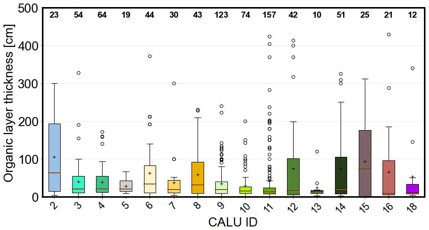
Figure 7 Soil surface organic horizon depth statistics for units with at least 10 data points. Box plot representing quartiles, median, mean as “+” and outliers as “°” for Circumarctic Land cover Units (CALU) based on in situ data. Number of samples per unit are shown at the top. For unit details and colours, see Table 2.

Soil organic carbon (SOC) and total nitrogen (TN) were lowest for the barren unit (CALU no. 21; Table A2). Unit no. 10 and 11 (moist tundra, abundant moss and shrubs) showed the highest SOC values, with more than 35 kg C m⁻².

AVA records, which provide wetness descriptions, included the categories wet and aquatic in more than 50 % of the samples in units no. 3, 4 and 8 (Fig. 6). Unit 15 (dry to moist tundra, partially barren) also had a comparably high fraction of moist and aquatic samples. The AVA records complemented the soil description specifically for unit no. 6 (only four pedon records). The AVA records confirmed that it is a relatively dry land cover type.

4.4 Fire disturbance assessment

The majority of input data for the land cover classification were acquired between 2017 and 2020. The assignment to the disturbance unit, unit no. 17, occurred up to 4 years after a burn event (Fig. 8). A specific year could not be determined in most cases due to averaging over up to 3 years. Burned areas from events before 2014 were represented through other units (vegetation recovery).

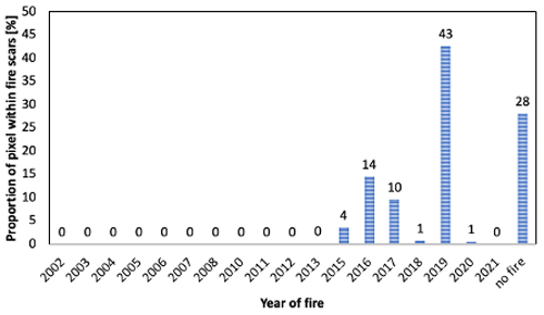
Figure 8 Year of fire for pixels in unit 17 (recently burned or flooded, partially barren) for Alaska (source: Alaska Large Fire Database).

The disturbance unit, unit no. 17, occurred within recently burned areas in approximately 72 % of all cases documented for Alaska. The majority of remaining unit no. 17 areas occurred along shorelines of lakes with varying extent. This was specifically the case on the Alaska North Slope (Fig. 9).

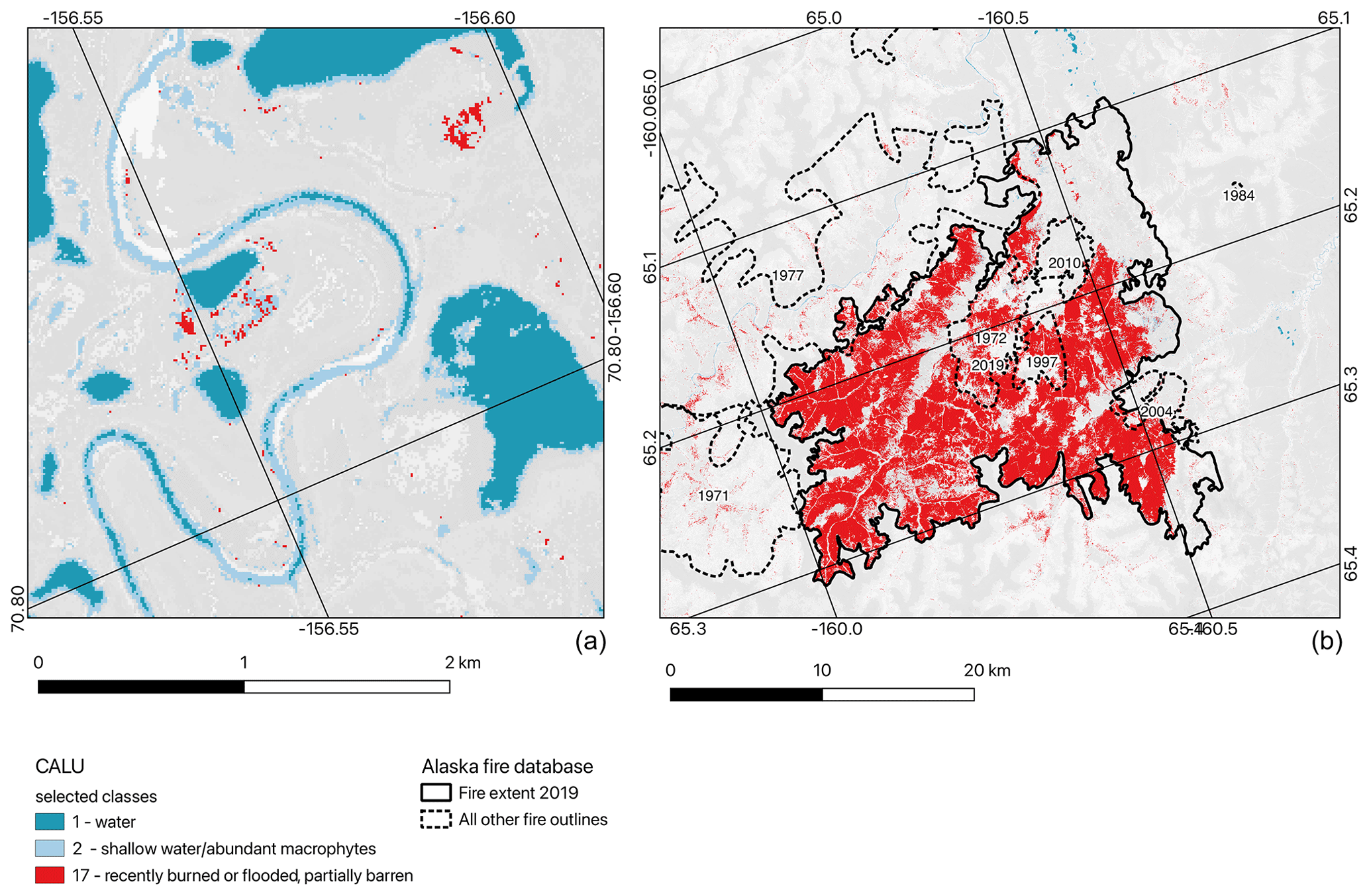
Figure 9 Examples for CALU no. 17 “recently burned or flooded” (shown in red). (a) Lakes within a river floodplain on the Alaska North Slope. (b) Burned areas in southwestern Alaska (outlines and years from Alaska Large Fire Database). Grey shades represent units other than no. 1, 2 and 17.

4.5 Heterogeneity

Land cover diversity (richness based on fractions – at least 1 % – within 1×1 km areas) was lowest in the higher Arctic and higher towards south (Fig. 10). The average number of land cover units ranged from four to nine, depending on the majority unit type. The barren-unit-dominated regions had the lowest richness (Fig. 11). Of the CAVM extent, 81 % had at least 1 % wetland within the 1×1 km cells (considering the sum of all types – units no.  2, 3 and 4), but only 0.7 % of the area constituted cells with pure wetlands. The average wetland fraction across the entire CAVM region was 8.8 %.

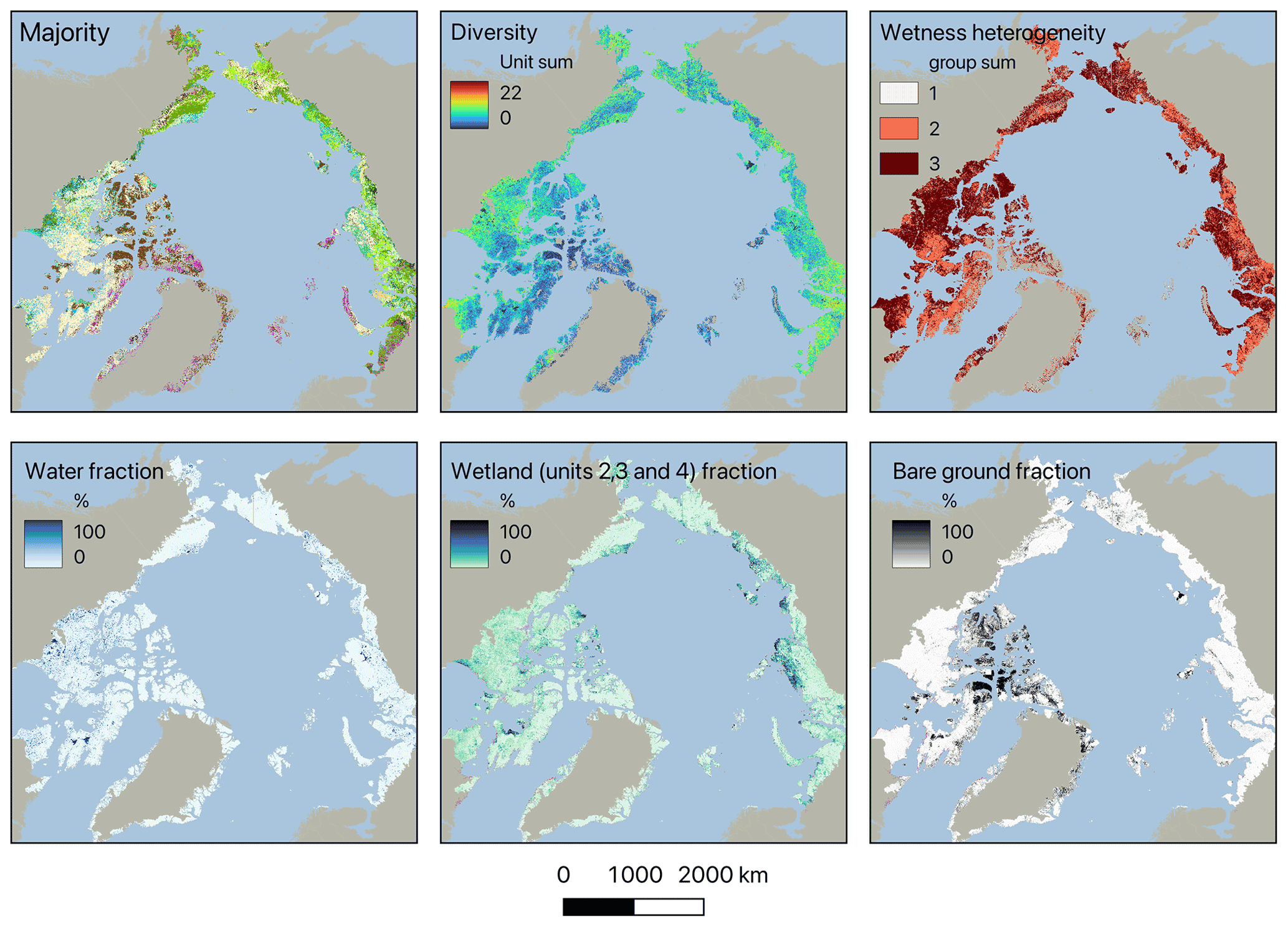
Figure 10 Statistics for CALU (10 m original resolution) for 1×1 km areas. For legend of majority, wetness groups and unit IDs, see Table 2.

The CAVM class W3 (sedge, moss, low-shrub wetland complex) showed the highest diversity, with almost nine units on average (Fig. 12). In general, wetter regions had a higher diversity than drier ones. This was also confirmed through the wetness group assessment. In 59 % of cases when wet types were present, dry and moist types were found at the same time. Of the CAVM extent, 66 % was heterogeneous regarding wetness (group sum 3, areas with no data excluded) and only 12 % homogeneous (group sum 1) (Fig. 13 left). The fraction of areas with a sum of three reduced when the heterogeneous unit, unit no. 6, was assigned to “moist” instead of “dry” but remained comparably high with 48 %.

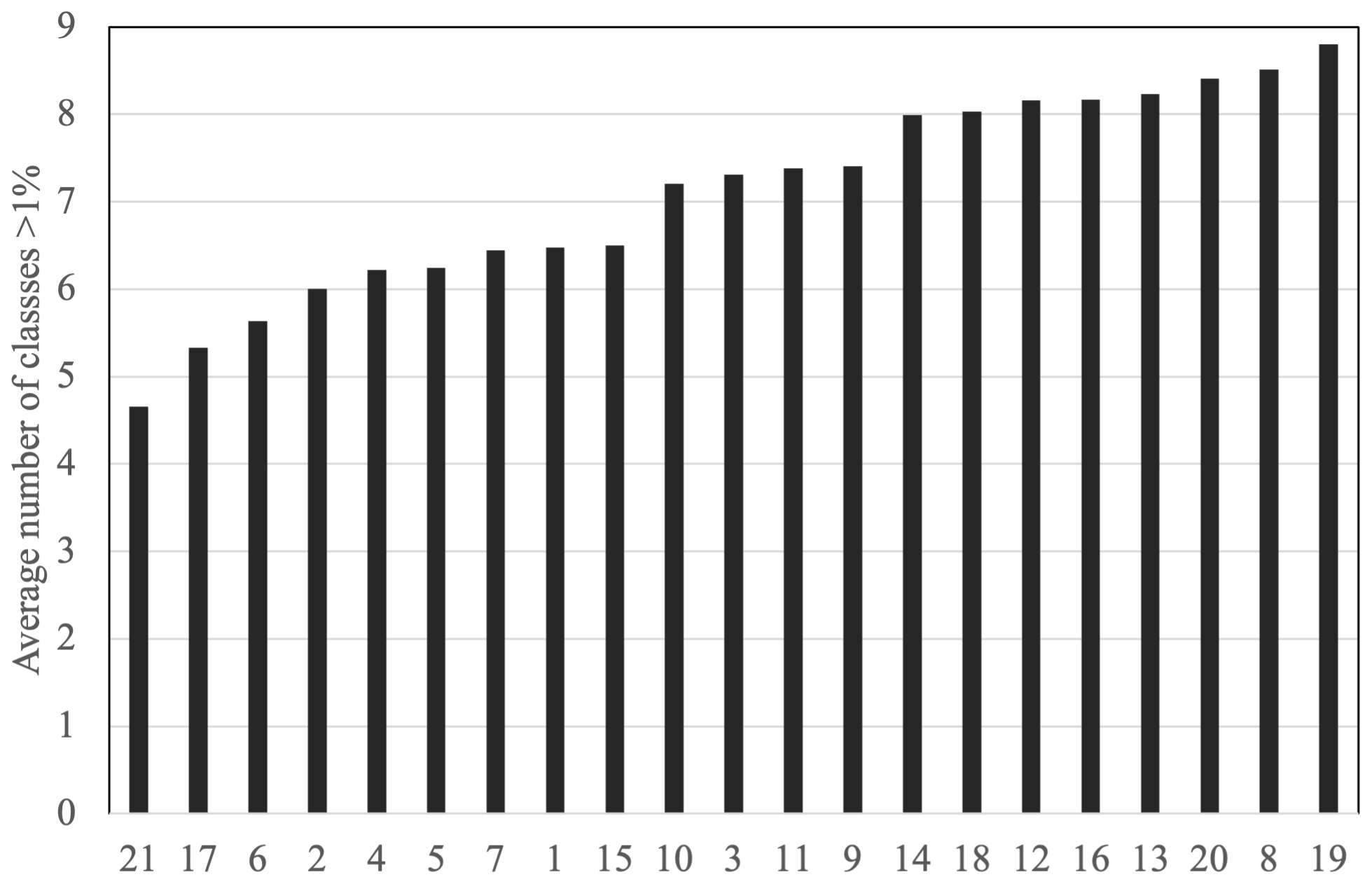
Figure 11 Diversity (average number of units (CALU) within 1 km × 1 km cells) versus majority; for unit IDs see Table 2. Sorted by diversity.

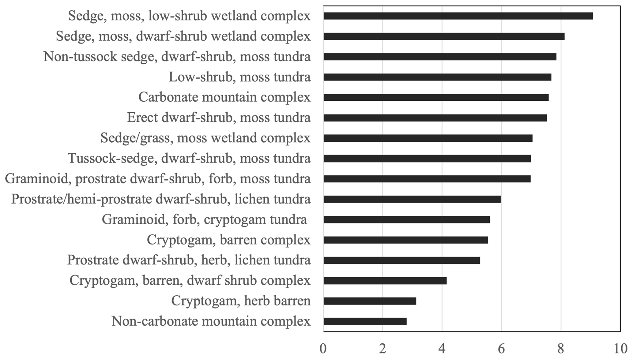
Figure 12 Land cover diversity for CAVM (Circumpolar Arctic Vegetation Map; (Raynolds et al., 2019)) classes: average number of units (CALU) within 1 km × 1 km cells.

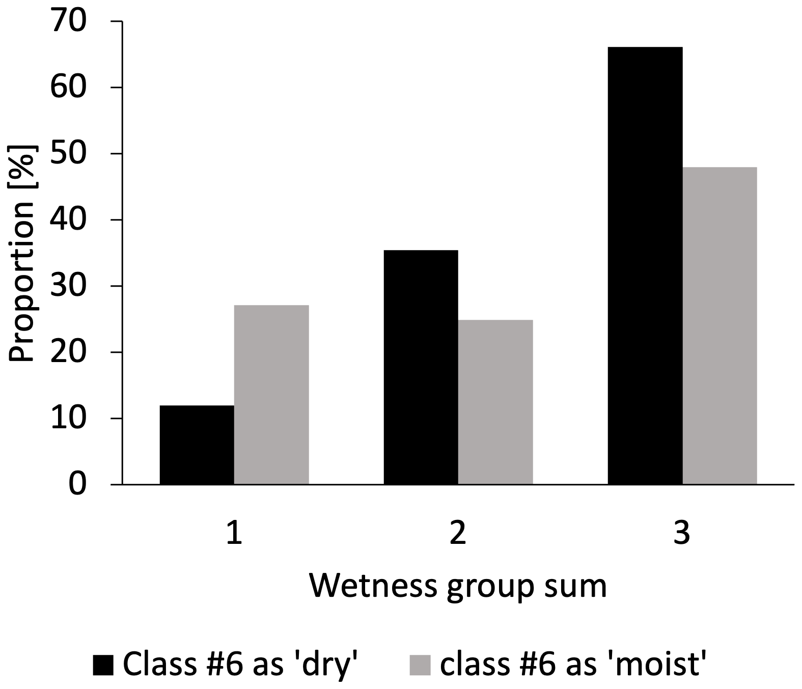
Figure 13 Wetness diversity within 1 km × 1 km areas (sum of groups B: dry, moist, wet; see Table 2; minimum 1 % fraction for each type), CAVM (Circumpolar Arctic Vegetation Map; Raynolds et al., 2019) region excluding areas with “no data”. Values for wetness group sum “1” are the proportion of 1×1 km areas that had only one wetness category, group sum “2” had two wetness categories and group sum “3” had all three.

4.6 Comparison with existing datasets

Subsets of selected regions in West Siberia, Alaska and Canada were investigated. This included regions with dwarf to low shrubs with patches of wetlands (Figs. 14 and 15) within the original prototype extent (see Fig. 1). The prototype (LCP; 20 m), CCI Land Cover (300 m), the CAVM (1 km) and CALC-2020 (10 m) were compared with CALU (10 m). Distinct differences were found between CALU and other land cover maps which are not only related to the spatial resolution difference. Wetland areas are considerably more extensive in the CALC-2020 (which is the only classification largely driven by terrain information) than in all other maps, including CALU. Wetlands are more extensive in CALU than in CCI Land Cover and CALC-2020 in the example from the Alaskan coastal plain (Fig. 16). Patterns are mostly similar for the example from the Tuktoyaktuk region (Fig. 17). Only CALC-2020 differs, where graminoids dominate instead of dwarf to low shrubs.

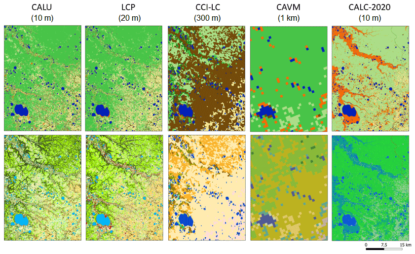
Figure 14 Comparison across all evaluated products for a region dominated by shrub tundra with patches of wetland (CALU – Circumarctic Land cover Units, LCP – land cover prototype, CCI-LC – Climate Change Initiative – Land Cover, CAVM – Circumpolar vegetation map, CALC – Circumpolar Arctic land cover 2020). Upper row – grouped classes (with name of source and spatial resolution), lower row – original classes (for detailed legend, see Tables 1, 2, C1, C2 and C3). For location, see Fig. 1 (number 1).

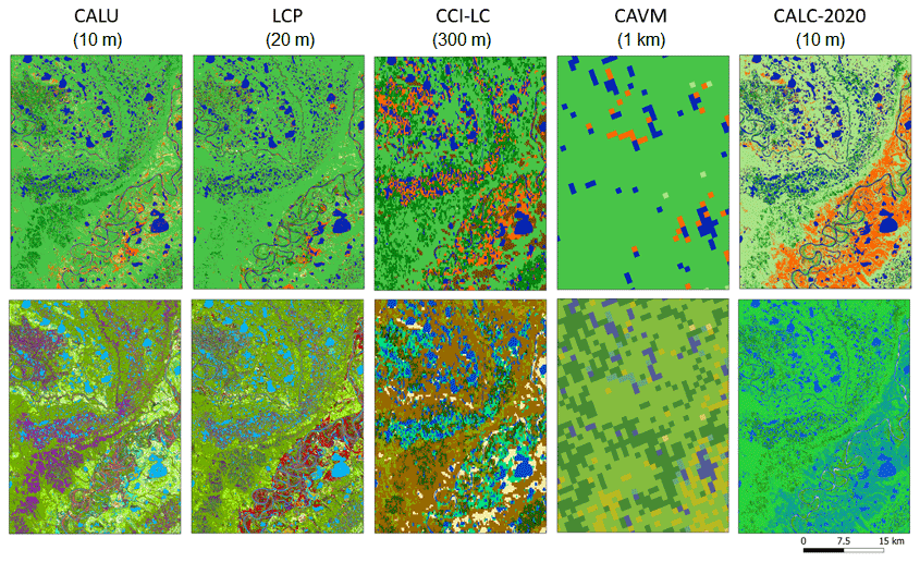
Figure 15 Comparison across all evaluated products for a region dominated by shrub tundra with patches of forest and wetland (CALU – Circumarctic Land cover Units, LCP – land cover prototype, CCI-LC – Climate Change Initiative – Land Cover, CAVM – Circumpolar vegetation map, CALC – Circumpolar Arctic land cover 2020). Upper row – grouped classes (with name of source and spatial resolution), lower row – original classes (for detailed legend, see Tables 1, 2, C1,C2 and C3). For location, see Fig. 1 (number 2).

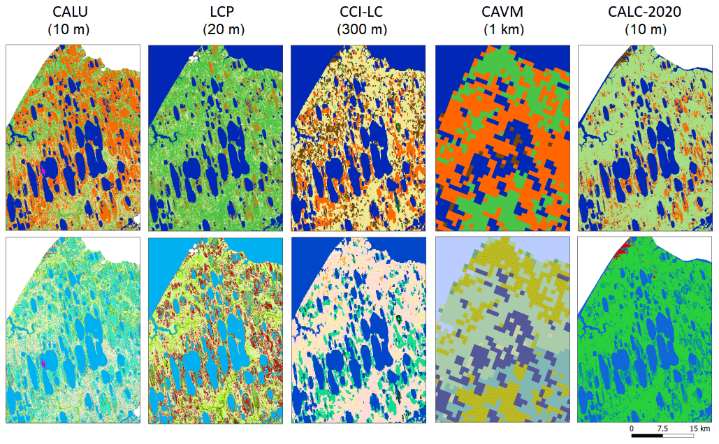
Figure 16 Comparison across all evaluated products for a region dominated by wetlands and lakes (CALU – Circumarctic Land cover Units, LCP – land cover prototype, CCI-LC – Climate Change Initiative – Land Cover, CAVM – Circumpolar vegetation map, CALC – Circumpolar Arctic land cover 2020). Upper row – grouped classes (with name of source and spatial resolution), lower row – original classes (for detailed legend, see Tables 1, 2, C1, C2 and C3). For location, see Fig. 1 (number 5).

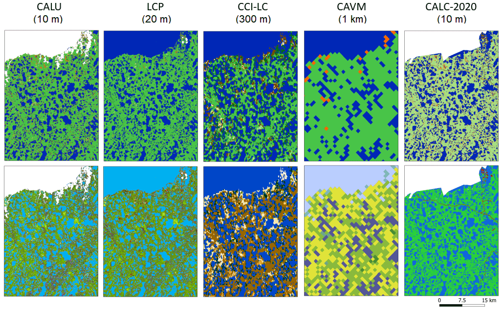
Figure 17 Comparison across all evaluated products for a region dominated by shrub tundra and lakes (CALU – Circumarctic Land cover Units, LCP – land cover prototype, CCI-LC – Climate Change Initiative – Land Cover, CAVM – Circumpolar vegetation map, CALC – Circumpolar Arctic land cover 2020). Upper row – grouped classes (with name of source and spatial resolution), lower row – original classes (for detailed legend, see Tables 1, 2, C1, C2 and C3). For location, see Fig. 1 (number 6).

4.6.1 Prototype

Results demonstrated the resolution difference between the prototype with 20 m and the CALU with 10 m well (Fig. 18). The patchiness of shrub tundra led to a reassignment to other vegetation units. About 15 % of the dwarf- to low-shrub tundra group was reassigned to other groups, mostly to wetlands (5 %) and graminoids/lichen/moss (5 %). The new disturbance units resulted in a shift of area from lichen/moss to the barren group (which was largely only partially barren according to the description of units (CALU)). Pixels originally classified as disturbed were assigned to vegetation units, specifically no. 8 (dry to aquatic tundra, with 42 %; Fig. D1). The maximum fraction of a prototype class within a new unit ranged from 17 % (disturbed) to 96 % (water) and was on average 50 %.

Figure 18 Proportion of grouped CCI Land Cover, CAVM, CALC-2020 and prototype classes within grouped units (CALU). For grouping schemes, see Table  2 and Table C3. Matrices are provided in Tables 4, C4 and C5 and as a sankey diagram in the case of the prototype (Fig. D1).

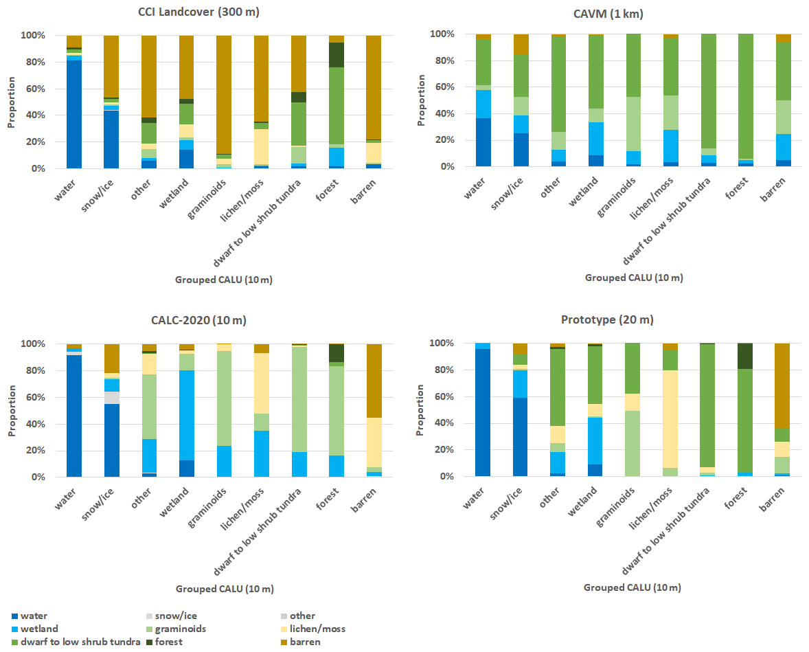
4.6.2 CCI Land Cover

The barren group of CCI Land Cover was predominant in all tundra vegetation groups of CALU (Fig. 18). In the lichen/moss group of CALU, less than 30 % was in the same group in CCI Land Cover. Also, the shrub and forest groups were most abundant in shrub tundra and forest respectively. More than 88 % of the CCI Land Cover barren group was actually characterized by vegetation (example maps in Figs. 14 and 15); 60 % was dwarf- to low-shrub tundra, about 9 % graminoids and 16 % lichen/moss (Table 4).

Table 4 Comparison matrix of grouped Climate Change Initiative (CCI) Land Cover classes and grouped units (Circumarctic Land cover Units – CALU). Values in percent. For grouping schemes, see Tables 2 and C1.

About 80 % of the CCI Land Cover class forest were in the shrub tundra group of CALU. The overlap applied specifically to unit 12, “dry to moist tundra, dense dwarf and low shrubs”. Low shrubs are abundant and very dense in the proximity to the treeline (see photograph in Fig. B39).

4.6.3 CAVM

The shrub tundra group of the CAVM was present with more than 40 % in all CALU groups (Fig. 18). This can be attributed largely to the spatial resolution difference. The spatial patterns were, however, similar (Figs. 14 and 15). Overlapping areas with the group forest corresponded mostly to shrub tundra as the CAVM does not have a forest class. Less than 1 % of CALU within the CAVM boundary was identified as mixed or needle leaf forest.

4.6.4 CALC-2020

There was a substantial mismatch between the two datasets for the group “dwarf- to low-shrub tundra” and “wetland” (Fig. 18). About 80 % of this group was labelled as graminoids and most of the remaining part to wetland in the CALC-2020. Large proportions of wetlands were also found in the CALU groups lichen/moss and forest as a larger proportion of the landscape.

5 Discussion

5.1 Adjustment of the prototype retrieval scheme

The high level of heterogeneity at the 1 km scale for shrub tundra and wetland complexes (as defined in the CAVM; Fig. 12) underlines the importance of spatial resolution and need for thematic content. The prototype was developed at 20m nominal spatial resolution as the 20 m bands of Sentinel-2 were used to better exploit the spectral capabilities. In this study, a super-resolution approach (convolutional neural networks) adjusted to Arctic environments was applied to bring these bands to 10 m. Nevertheless, the original 20 m resolution might contribute to issues in unit representation at 10 m due to the high heterogeneity.

The re-assignment of the units between the prototype and CALU reflects the high heterogeneity. The largest differences in unit assignment between the prototype with 20 m and the new version with 10 m occurred for the shrub tundra groups (Fig. D1). The splitting of the “disturbed” unit into two resulted in re-assignments across more types than initially foreseen (Fig. D1). Pixels were also re-assigned to wetlands, the heterogeneous units, unit no. 8 (dry to aquatic tundra) and unit no. 6 (dry to moist prostrate shrub tundra, partially barren), in addition to the new units, unit no. 15 (dry to moist tundra, partially barren) and unit no. 17 (disturbed, including burned areas). Unit no. 15 also now consists of areas previously assigned to no. 6. All partially barren units might potentially include disturbed areas, for example, wind-blown sands and landslide scars, as common across the Yamal Peninsula.

5.2 Expansion of the approach across the Arctic

Environmental conditions distinct from West Siberia occur specifically where coastal plains and river deltas can be found. Nevertheless, example comparisons with other circumpolar/global maps for the Alaska North Slope (coastal plain) and the Canadian Tuktoyaktuk Peninsula document similar results to those for West Siberia.

Regional maps which offer comparably high thematic content are available in other parts of the Arctic, especially for North America. These are, however, based on Landsat. The lower spatial resolution (30 m) does therefore limit the applicability for cross-validation on their basis. Several units are expected to be assigned to the classes due to land cover heterogeneity. Examples are provided in Figs. S2 and S3 in the Supplement.

The high number of units requires cloud-free Sentinel-2 at the peak vegetation season. A period of several years is therefore needed to assemble the circumpolar mosaic. Ingested images span a wide range of acquisition years, which may limit application of land cover change studies. Such analyses should be carried out only locally and the documentation of acquisition dates consulted. In addition, years can differ regarding land surface hydrology and vegetation state. Wet years with flooding and dry years leading to drought are expected to impact the detectability of especially the wetland units. Haze caused by forest fires in general cannot be corrected with the tools used. Affected scenes can not be used. This reduces the number of usable scenes considerably, as fires are abundant in the boreal forest, and smoke is transported to adjacent tundra areas.

Issues with wrong assignment are common for lakes in the northern parts. Late floating ice fragments are identified as ice/snow instead of open water. The snow/ice class can, however, be re-labelled as water in regions without glaciers (excluding High Arctic islands, Greenland and mountain ranges). Lakes may also be missing in regions close to the coastline where the Copernicus DEM contained zero or no data. Tree species typical of forest occur with reduced size, crown diameter and sparse distribution in the transition zone. Several units which include low shrubs may therefore also include trees.

The current CALU version and presented analyses do not distinguish between natural and artificial barren areas, but a dataset which can be used for separation is available (Bartsch et al., 2021a, b). It was derived from Sentinel-1/Sentinel-2 at 10 m nominal resolution. The fraction of artificial areas over the analyses region is, however, comparably small, < 0.02 % versus an overall barren fraction of 14.5 % (Table 2).

5.3 Separation of wetlands

Wetlands (in addition to lakes; Matthews et al., 2020) are of high relevance for permafrost studies as moisture gradients determine carbon fluxes, specifically potential release of methane. The three wetland types represent distinct environments with respect to hydrology and nutrient status. The total nitrogen density of no. 3 (permanent) is lower than for no. 4 (seasonal) (Table A2). Unit no. 2 represents permanent inundation. In addition, land cover unit composition and spatial patterns may allow for separation of different wetland types. In particular, unit no. 8 is expected to be very heterogeneous and to include inundated parts (see AVA records in Fig. B21). Figure 19 provides examples for different patterns of wetland units. Drained lake basin composition is distinct from wet sites in areas dominated by peat bogs. The occurrence of wetland units no. 3 (permanent) and no. 4 (seasonal) also differs across different wetland landscapes (wetscapes as defined in Olefeldt et al., 2021, Fig. S4).

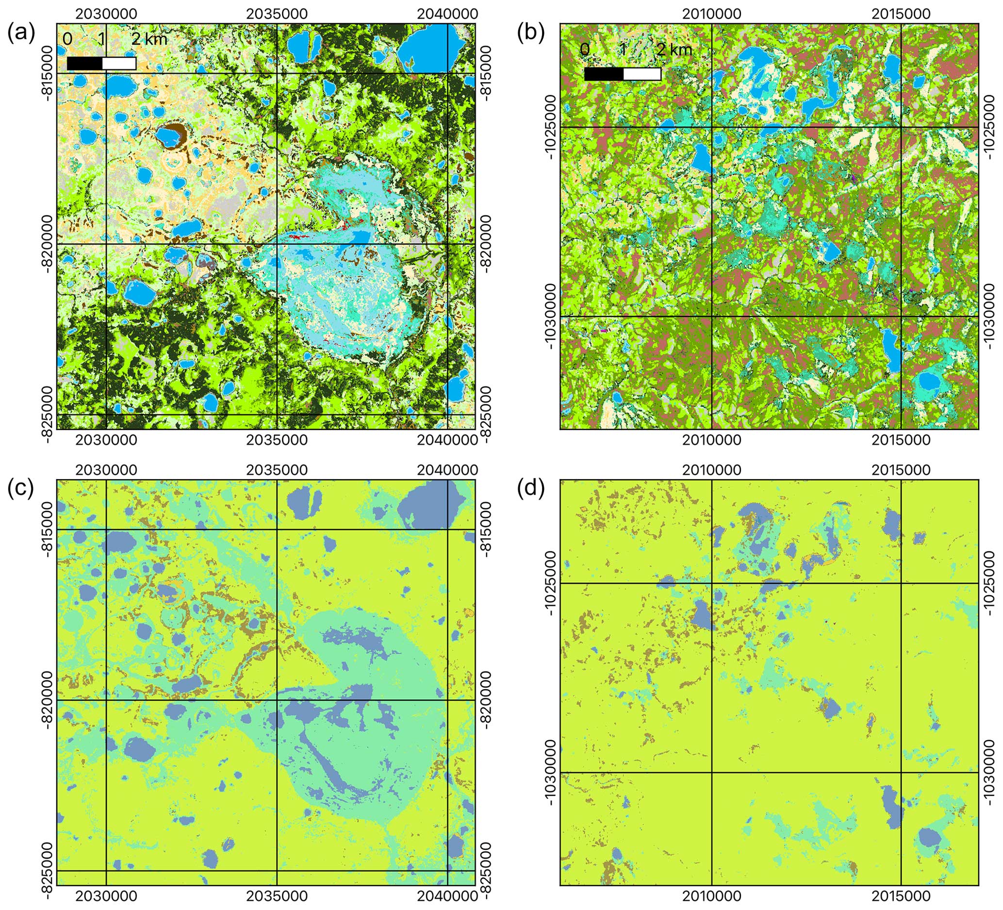
Figure 19 Examples for different wetland types: (a, c) drained lake basins on central Yamal in the tundra zone (wetscape “wetland and lake-rich tundra” according to Olefeldt et al. (2021); see also Fig. S4) and (b, d) peat bogs in the hypo-Arctic tundra zone of West Siberia (wetscape “upland tundra” according to Olefeldt et al. (2021); see also Fig. S4). (a, b) CALU – for legend, see Table 2. (c, d) CALC-2020 (Liu et al. (2023), blue – open water, turquoise – wetland, light green – graminoid tundra, brown – barren; for detailed legend, see Table C3).

5.4 Implications for estimating soil organic carbon and wetland extent across the Arctic

Previous studies used CCI Land Cover for estimation of wetland area and soil organic carbon content across the Arctic, but concerns were raised by Palmtag et al. (2022). The comparison between CALU and CCI Land Cover confirms a previous assessment which used Landsat-derived regional land cover maps (Bartsch et al., 2016a). The thematic content does not match tundra-specific landscape types. The barren fraction is in general too large. A large proportion is covered by low vegetation.

Palmtag et al. (2022) used CCI Land Cover for the upscaling of soil organic carbon. Soil probe data were linked with the land cover units. An average of more than 9 kg C m⁻² over the top metre was calculated for the barren classes, which is much higher than in the CALU assessment (2 kg C m⁻²) due to occurrence of in situ sites representing organic soils in the CCI Land Cover barren class.

The agreement between the wetland classes of CCI Land Cover and CALU was very low, which confirms the assessment based on in situ observations by Palmtag et al. (2022) (20.65 % (Table 4) and 19 % respectively). This has implication for further use as for example in the case of wetland map creation such as in Olefeldt et al. (2021). Palmtag et al. (2022), with reference to Hugelius et al. (2020), suggest a permafrost wetland area 4 times larger. The underestimation of wetland extent in CCI Land Cover can be confirmed with CALU. Just within the extent of the CAVM, our estimate (1.16×10⁶ km²) is larger than the CCI Land Cover fraction for the entire high-latitude permafrost domain (1.01×10⁶ km²).

The use of terrain information in the retrieval as in the CALC-2020 dataset leads to overestimation of wetland areas in valleys (Figs. 14 and 15) and drained lake basins (Fig. 19). The heterogeneity in those areas is lost in this case. In total, more area is, however, characterized by wetland in CALU. This might be attributed to the inclusion of shallow water bodies with abundant macrophytes (unit no. 2).

5.5 Description of units with in situ records

Although a very high number of in situ data were available (almost 40 times more vegetation sites than used for the CALC-2020 assessment; Liu et al., 2023), more is needed for full characterization of Arctic landscapes. The vegetation records used represent sites across West Siberia only. The available soil data were collected from regions spread across the Arctic, but there is a lack of data (organic layer thickness) for barren areas and for unit no. 13 (dense shrubs) as it is less common and more difficult to access. The latter also applies to the shallow water wetland unit (no. 2) as it is aquatic and thus usually not part of terrestrial surveys. This unit might be, however, important for the upscaling of methane fluxes. Soil data availability largely represents unit abundance. The most soil data are available for the second most common unit (no. 11) but much less for the most abundant unit (no. 6), which is most likely due to the comparably low organic carbon content and occurrence in High Arctic regions. Soil sampling usually targets soil carbon quantification. Shrub tundra types are in general well sampled (more than 50 % of records). Probes for organic layer thickness largely come from selected environments, often river floodplains (e.g. Lena Delta, Kytalyk) or drained lake basins (e.g. Alaska North Slope). Data for wet unit types (no. 3–5) mostly come from these type of sites. Paludification is therefore comparably low. Organic layer depth was thus rather low for these units. Unit no. 15 had rather high organic layer depth (Fig. 7) but only 25 samples and with a high spread and high mineral volumetric content. In addition to the use of more in situ data and region-specific retrieval, a stratified random selection of soil probes representing a diversity of settings might be eventually required to allow for the upscaling of soil properties.

Several units represent diverse moisture gradients according to the in situ comparison. This applies specifically to no. 8. This demonstrates that 10 m is insufficient to fully resolve Arctic land cover heterogeneity, confirming the findings of Virtanen and Ek (2014), Siewert et al. (2015) and Treat et al. (2018). There are also uncertainties in geolocation of both the satellite product and the in situ data. The representation of the in situ description for the 10×10 m is also an issue. This mismatch may play a role in the spread of properties within a unit and results in the fuzzy/broad naming of the units.

Group assignment was moist in most cases where dry to moist conditions were observed using both AVA and soil pedon records except for no. 6. This was justified based on the comparably high coverage with lichen and relatively low soil water content and high mineral content values in the pedon records. The previously published CAWASAR (CircumArctic Wetlands based on Advanced Aperture Radar; Widhalm et al., 2015) dataset also offers classes for dry, wet and moist soil. The majority of no. 6 areas coincides with the class “dry” (see Fig. S1), which confirms the validity of the group assignment. The comparison to the Alaska land cover map by Raynolds et al. (2017) and the Boreal-Arctic Lakes and Wetland Dataset (BAWLD) by Olefeldt et al. (2021) (Figs. S3 and S4) also shows that no. 6 mostly occurs in upland and alpine landscapes.

5.6 Application potential

We have provided descriptions of the CALU units based on a limited set of in situ records. Use of CALU subsets, especially outside of the regions with data availability as shown in Fig. A1, might require use of additional in situ records, specifically regarding soil conditions including organic layer thickness.

The high spatial and thematic detail of CALU potentially allows for space-for-time approaches of impact assessment of permafrost-related land cover change in addition to classical vegetation index trend analyses, for example, Nitze et al. (2018) and Foster et al. (2022). Disturbances related to abrupt thaw features are widespread across the Arctic. For example, vegetation is removed due to thaw slumping. Lakes drain and allow for vegetation regrowth. Both result in specific vegetation succession patterns, not only regarding vegetation types but also wetlands (Wolter et al., 2024). This has implications for carbon cycling. CALU in combination with records of disturbance timing (representing different stages) may support the quantification of abrupt thaw impacts.

6 Conclusions

Tundra regions with wetlands are characterized by high land cover diversity, in addition to the high number of small lakes. Wet, moist and dry landscape types co-occur close to each other in most of the area north of the treeline. Pure wetland coverage over an extent of 1×1 km is rare. This is expected to be of relevance for any type of analyses related to carbon fluxes, including up-scaling, inversions or land surface modelling.

Permafrost degradation features are known to lead to changes in land cover type and, specifically, wetness. For example, drained lake basins and also fire scars represent fast changing environments in the years after events. The new circumpolar land cover unit map provides three types of wetland units in addition to 14 terrestrial tundra units covering barren area as well as different types of shrub physiognomy and soil moisture gradients at 10×10 m. This level of detail is unprecedented. Both vegetation and soil type variations can be documented with extensive in situ datasets. Some land cover units with less extensive coverage, specifically disturbed sites (fires), are under-represented in available records.

The high thematic content requires good quality of input data. Although data availability from Sentinel-1 and -2 is good for 2016 onwards, the 7 years of records was not sufficient for complete coverage. CALU only covers 97 % of the Arctic (excluding ice sheets). Cloud coverage in the case of Sentinel-2 and inconsistent acquisition strategies for Sentinel-1 lead to quality issues. Several years' data from Sentinel-2 were combined for robustness where sufficient acquisitions were available. This needs to be considered when combined with other records, specifically with respect to assessment of cryosphere change impacts on land surface hydrology.

Appendix A: Selected statistics from in situ measurements

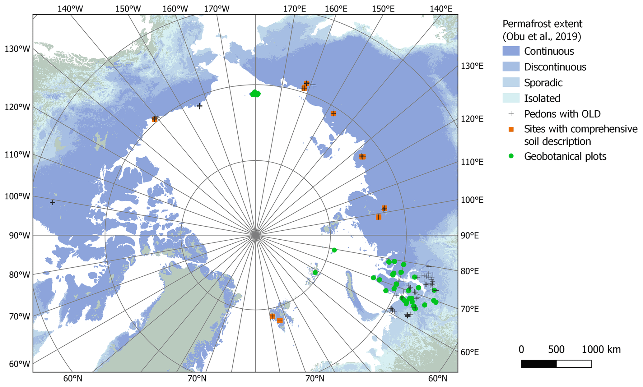
Figure A1 Location of in situ records (vegetation, Zemlianskii et al., 2023, and soils, Hugelius et al., 2013, 2014, 2020; Palmtag et al., 2022) and permafrost extent (source: Obu et al., 2019). OLD – organic layer depth.

Table A1 Soil surface organic horizon depth statistics extracted from several different sources, including Hugelius et al. (2013, 2014, 2020) and Palmtag et al. (2022).

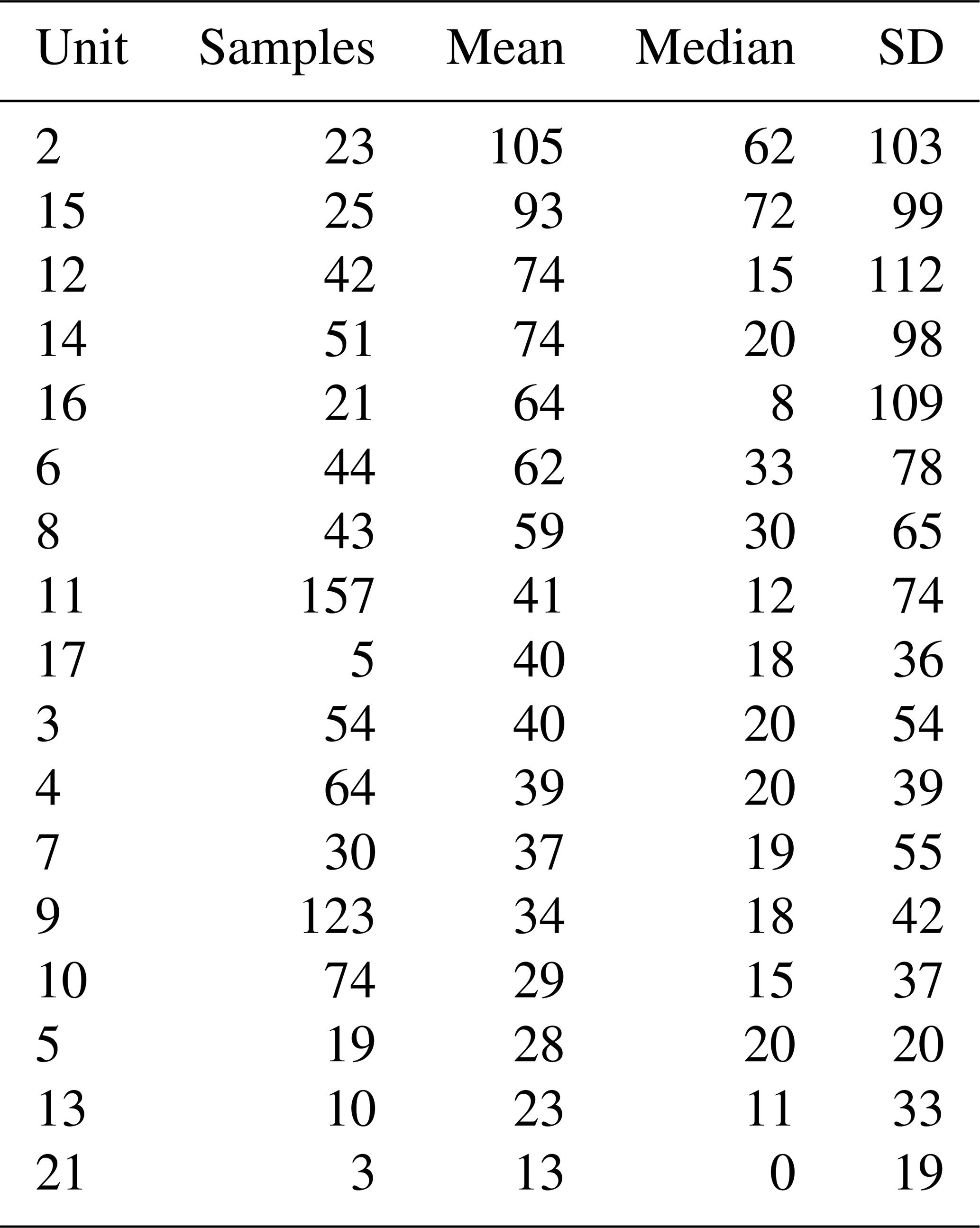
Table A2 Average soil characteristics based on Palmtag et al. (2022).

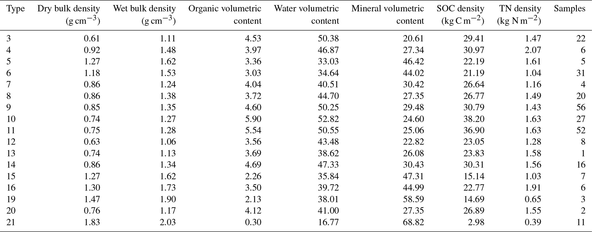
Table A3 Average coverage percentages per unit for vegetation types of used sites of the Russian Arctic Vegetation Archive (AVA; Zemlianskii et al., 2023).

Appendix B: Unit descriptions based on in situ samples

B1 CALU no. 1

Description. Open water.

B2 CALU no. 2

Description. Shallow water, abundant macrophytes.

Figure B1 CALU no. 2 vegetation properties based on AVA (Zemlianskii et al., 2023).

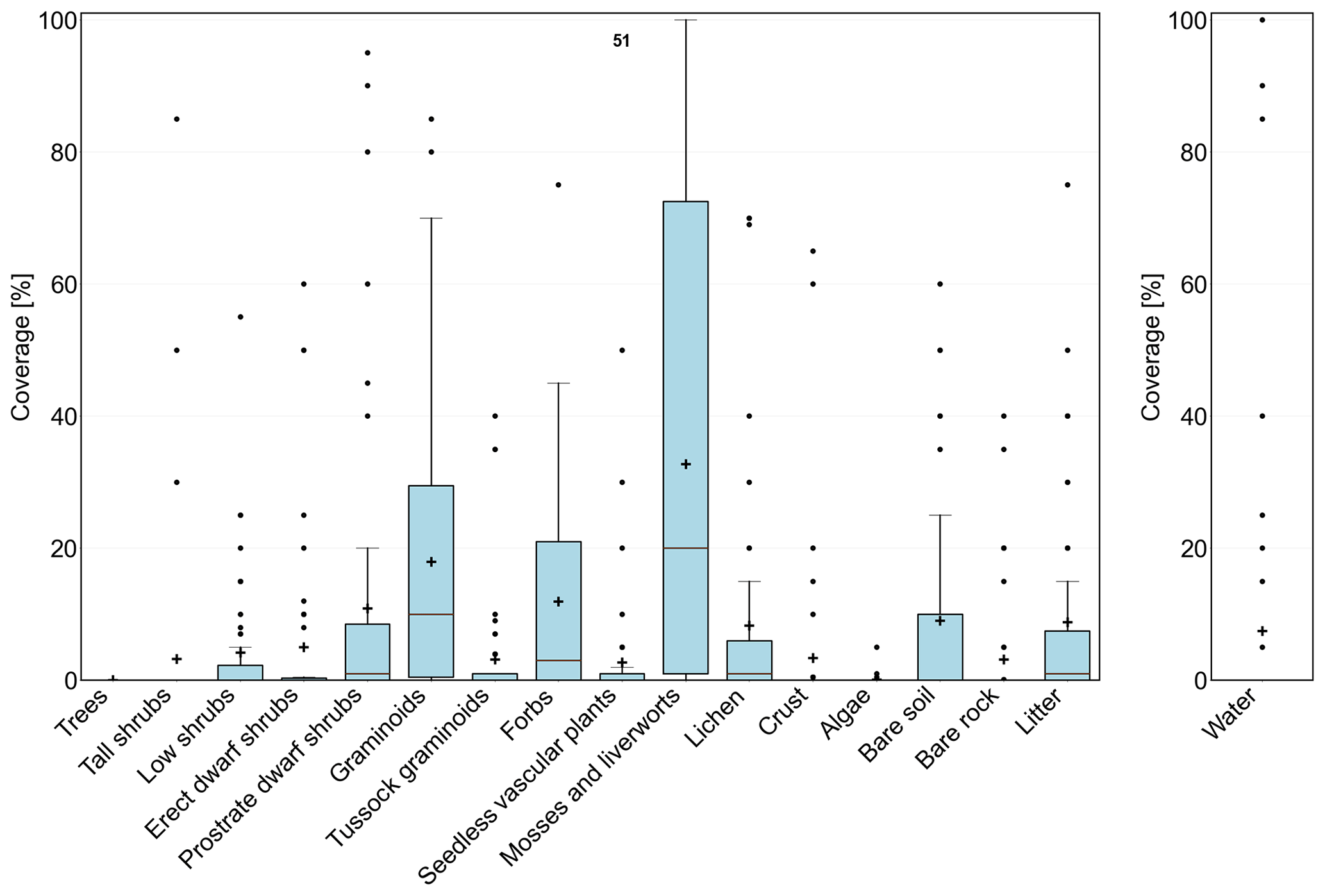
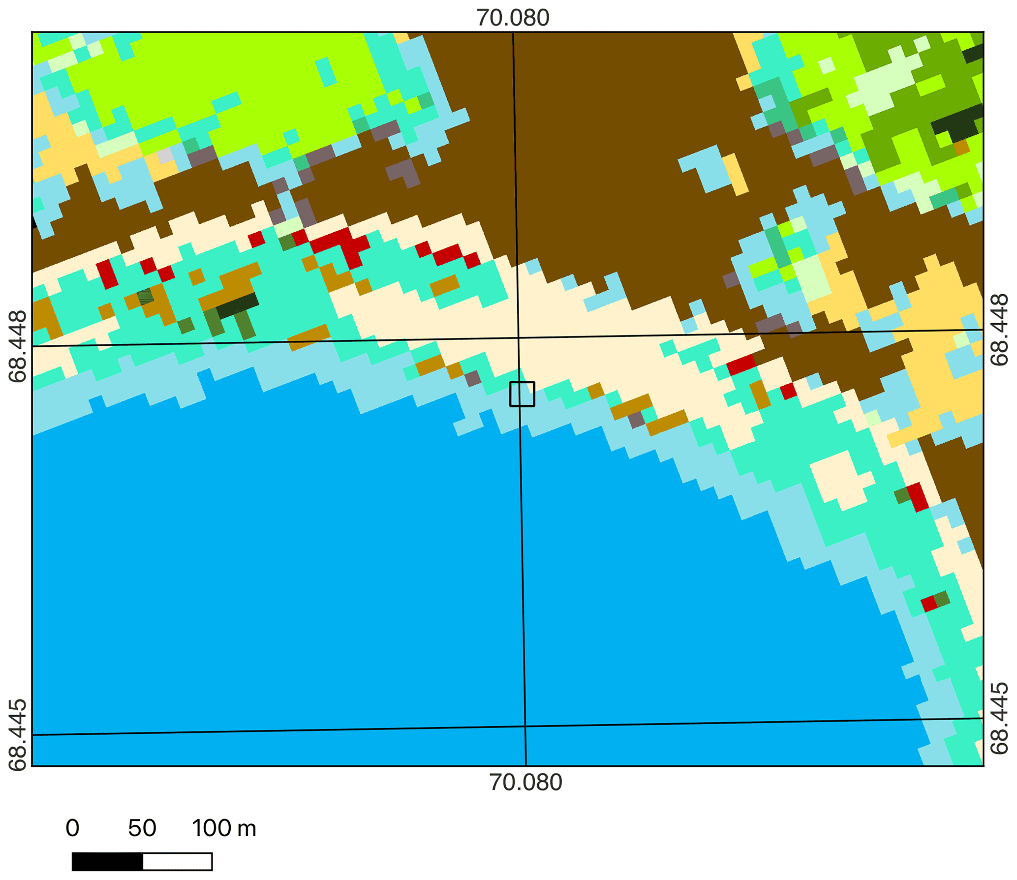
Figure B2 Example of a typical vegetation plot (Zemlianskii et al., 2023) located along a lake margin (square), falling into unit no. 2 (light blue; for full legend, see Table 2). In situ values: 15 % land covered by mostly graminoids, occurrence of 1 % forbs with height 50 cm, 85 % water, wetness category “moist”.

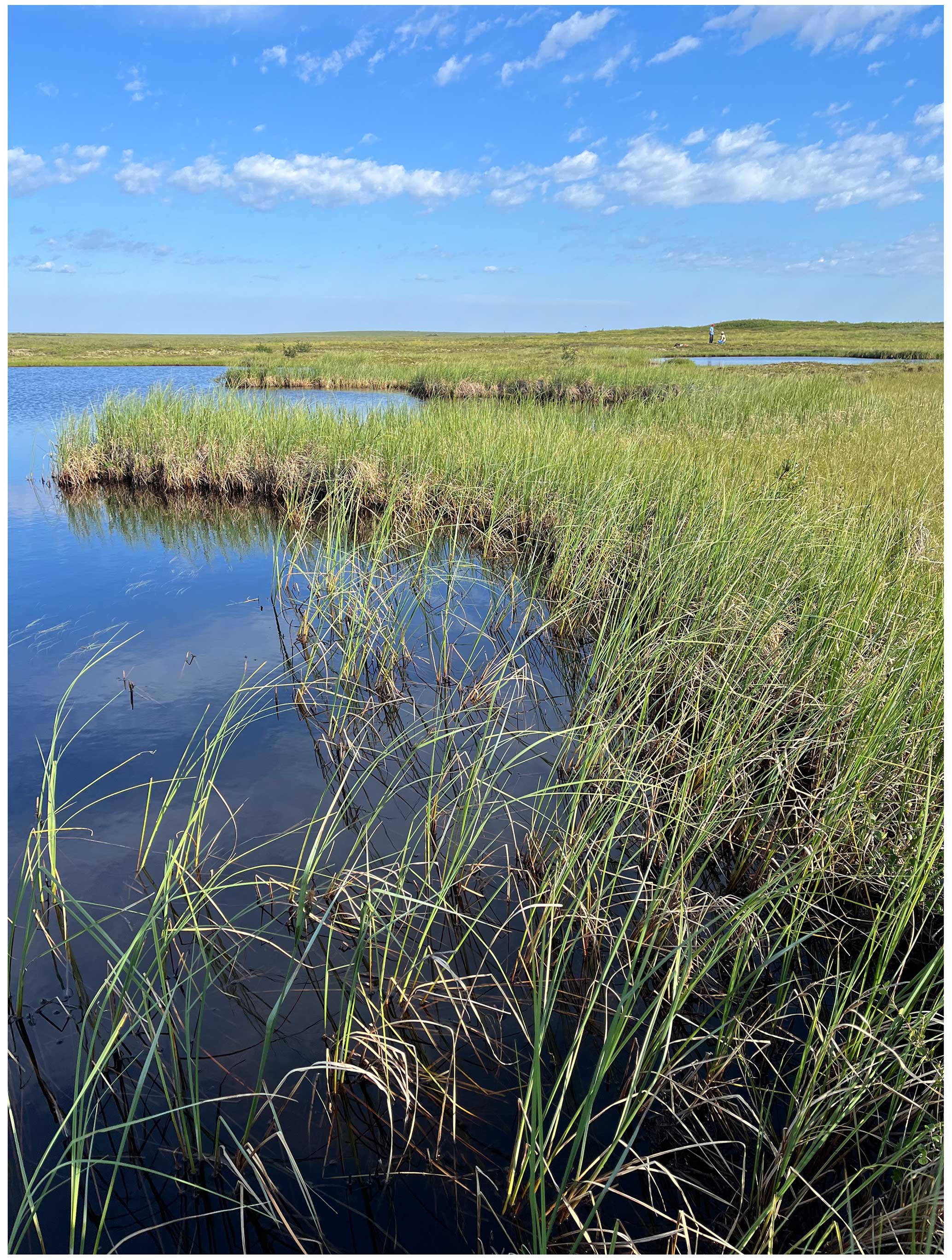
Figure B3 Example photograph CALU no. 2, lake margin with patches of macrophytes, water depth approximately 22 cm (Annett Bartsch, 21 July 2023; Inuvik region).

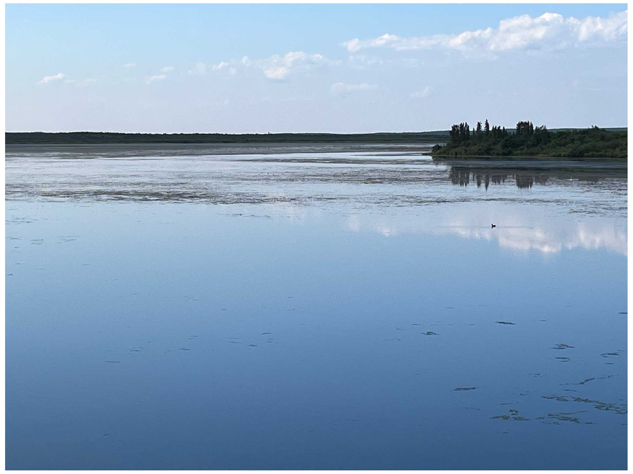
Figure B4 Example photograph CALU no. 2, lake with patches of macrophytes in the centre (Annett Bartsch, 21 July 2023, Inuvik region).

B3 CALU no. 3

Description. Permanent wetland, aquatic, low to medium organic layer thickness, medium mineral volumetric content.

Figure B5 CALU no. 3 vegetation properties based on AVA (Zemlianskii et al., 2023).

Figure B6 CALU no. 3 soil properties based on Palmtag et al. (2022).

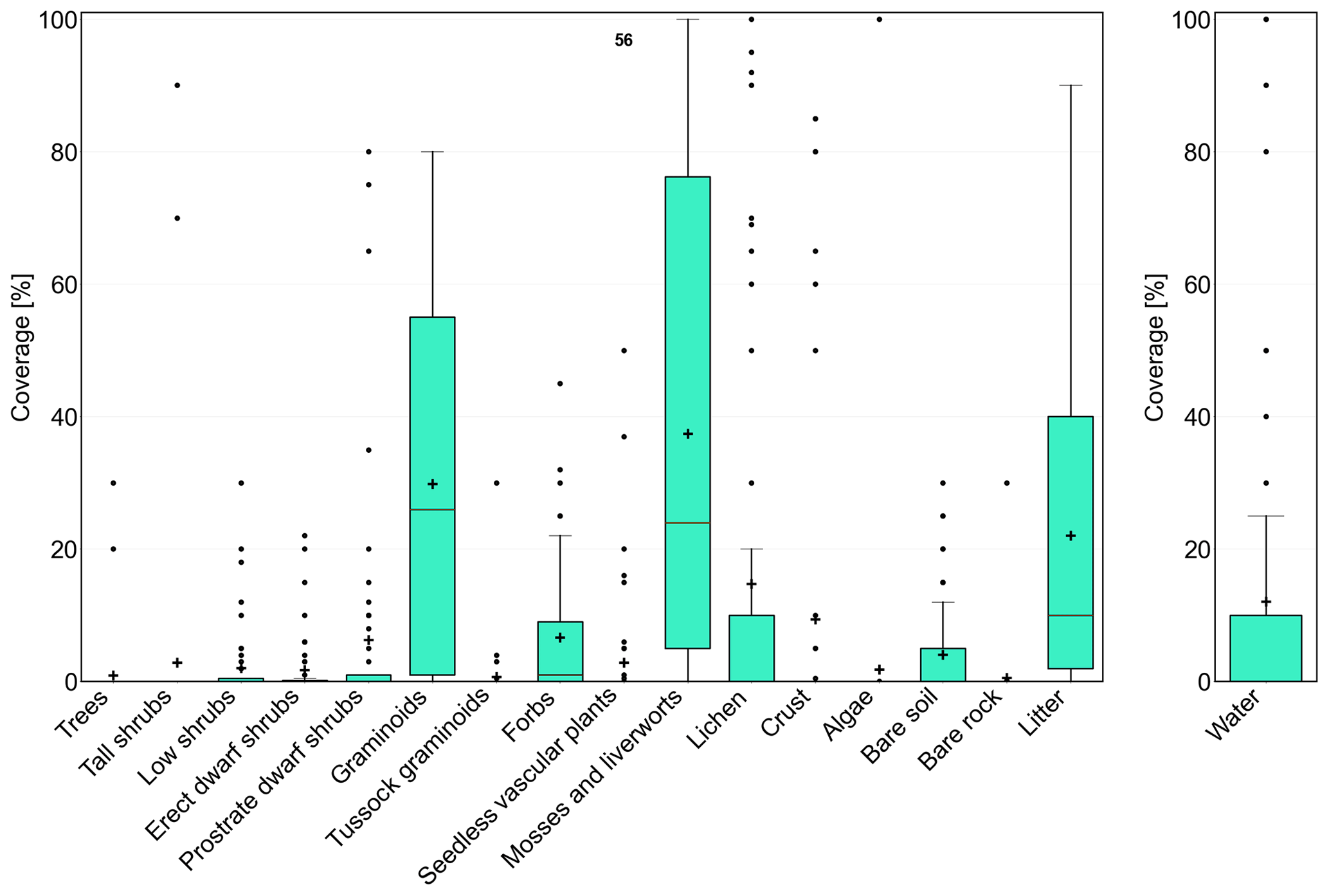
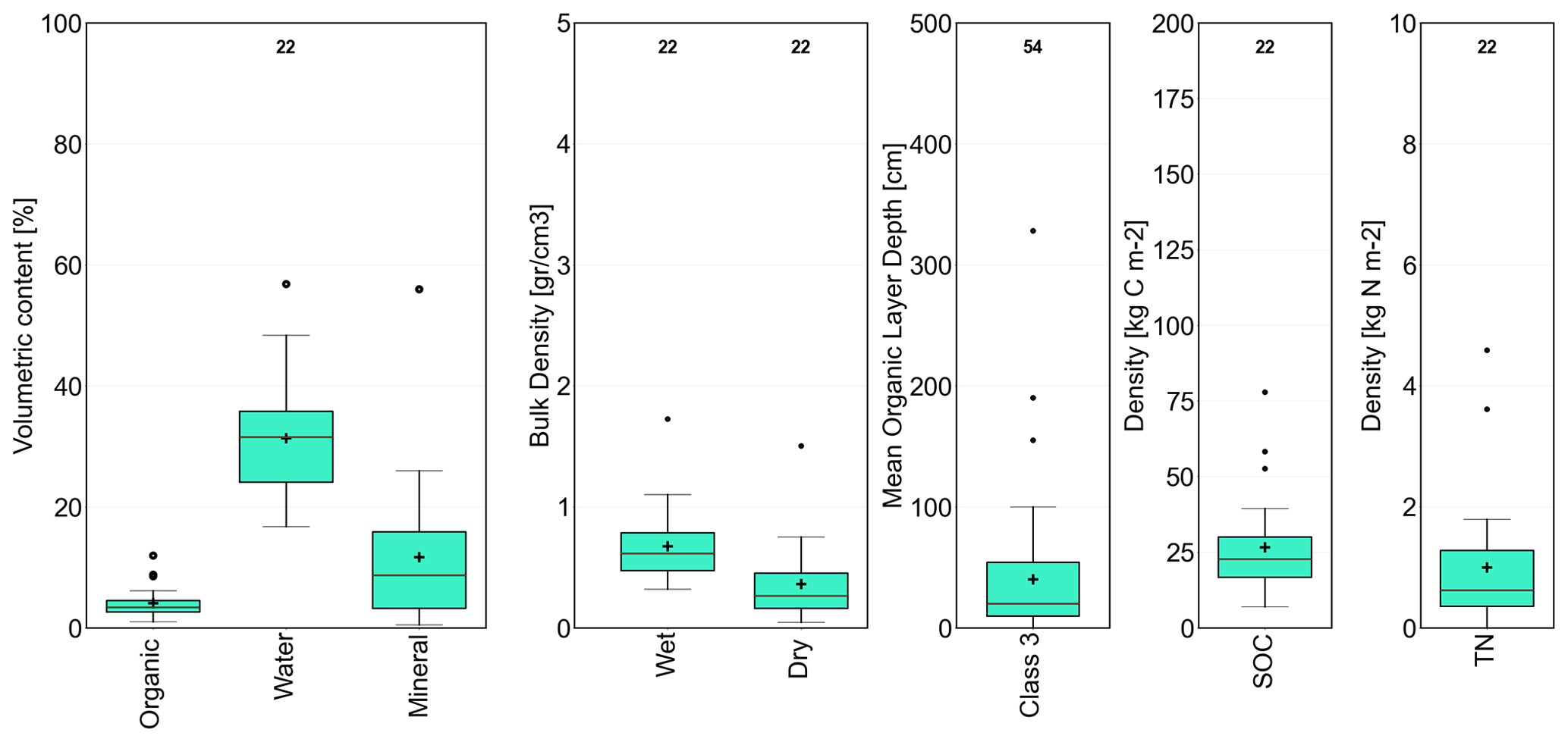
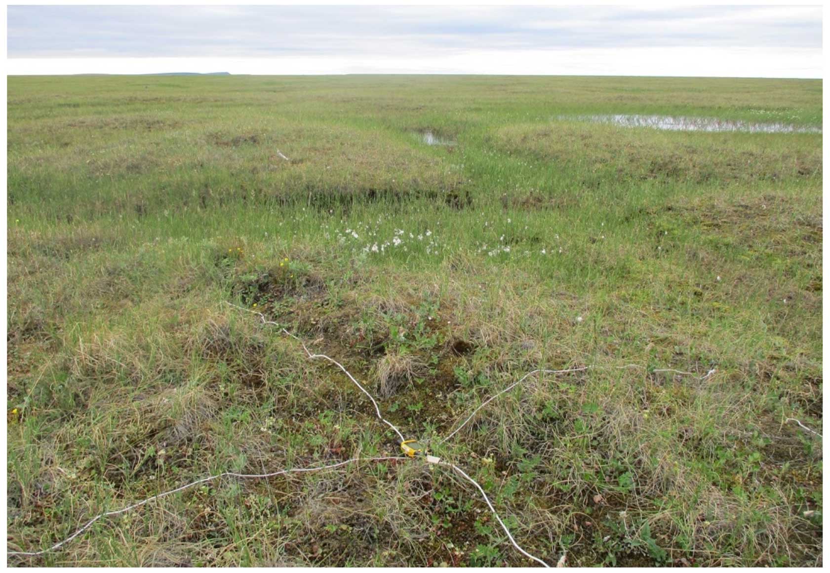
Figure B7 Example photograph CALU no. 3 (Birgit Heim, 12 July 2019; Lena Delta, Samoylov polygonal tundra).

Figure B8 Example photograph CALU no. 3 (Annett Bartsch, 21 July 2023; Inuvik region).

B4 CALU no. 4

Description. Wet to aquatic (seasonal wetland), abundant moss, low to medium organic layer thickness, low mineral volumetric content.

Figure B9 CALU no. 4 vegetation properties based on AVA (Zemlianskii et al., 2023).

Figure B10 CALU no. 4 soil properties based on Palmtag et al. (2022).

B5 CALU no. 5

Description. Moist to wet tundra, abundant moss, prostrate shrubs, low to medium organic layer thickness, medium mineral volumetric content.

Figure B11 CALU no. 5 vegetation properties based on AVA (Zemlianskii et al., 2023).

Figure B12 CALU no. 5 soil properties based on Palmtag et al. (2022).

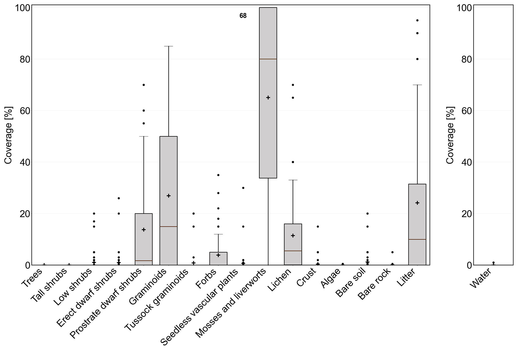
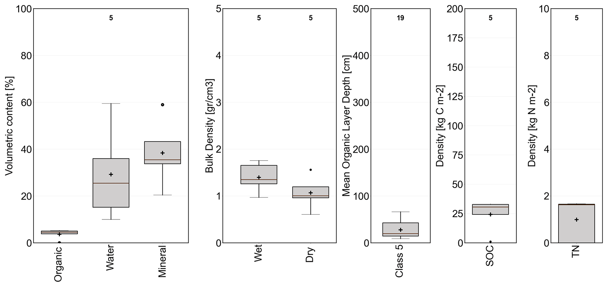
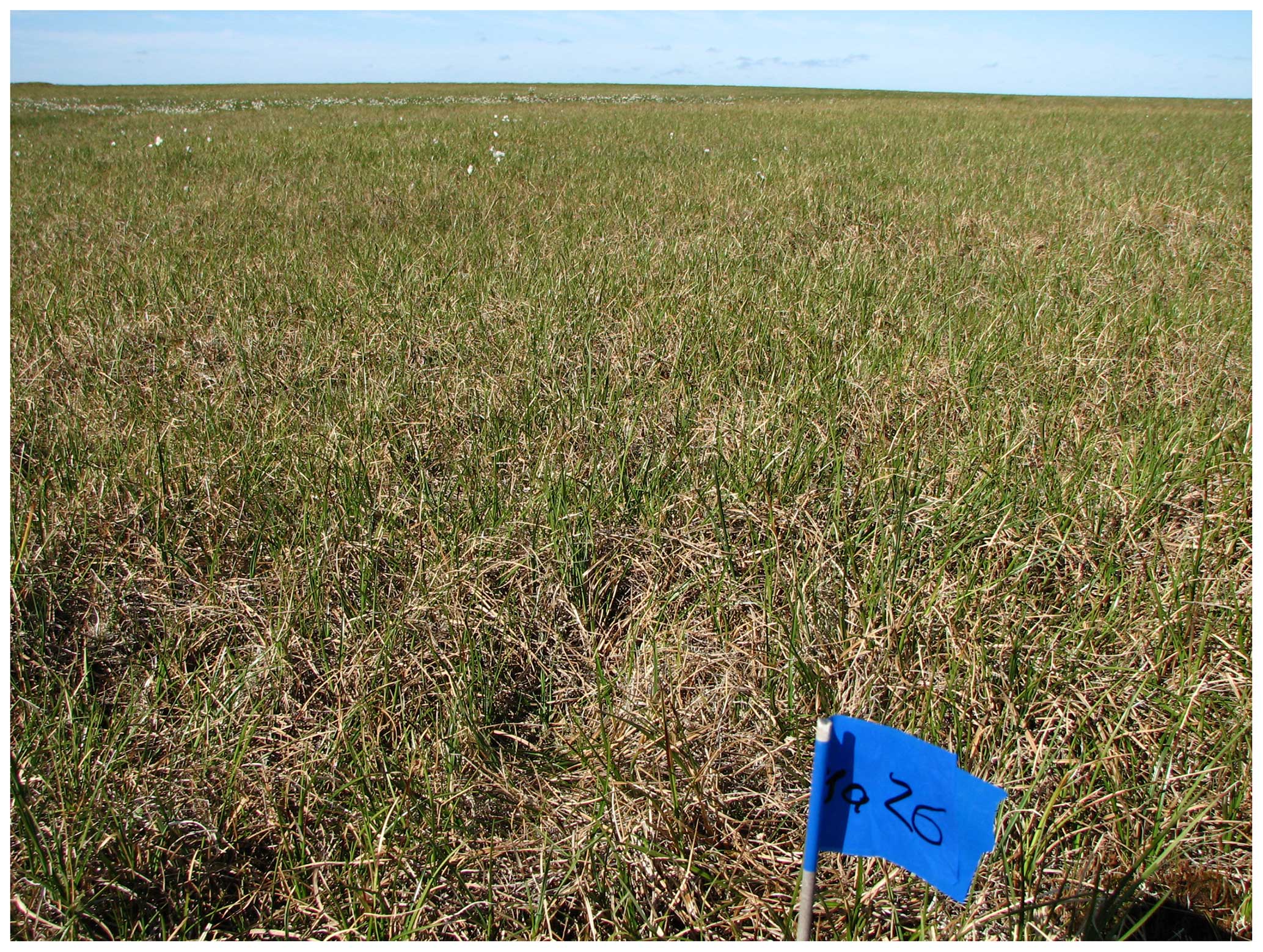
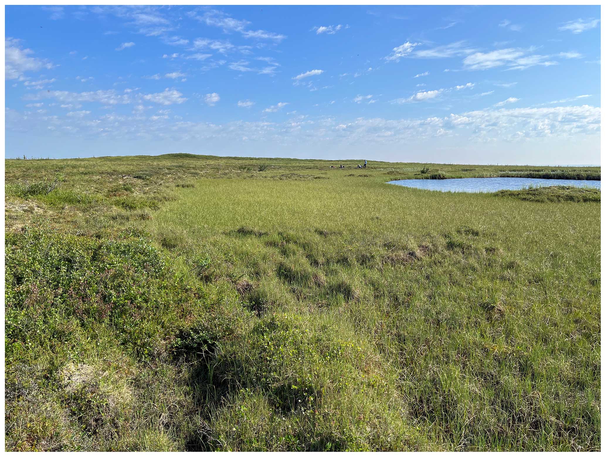
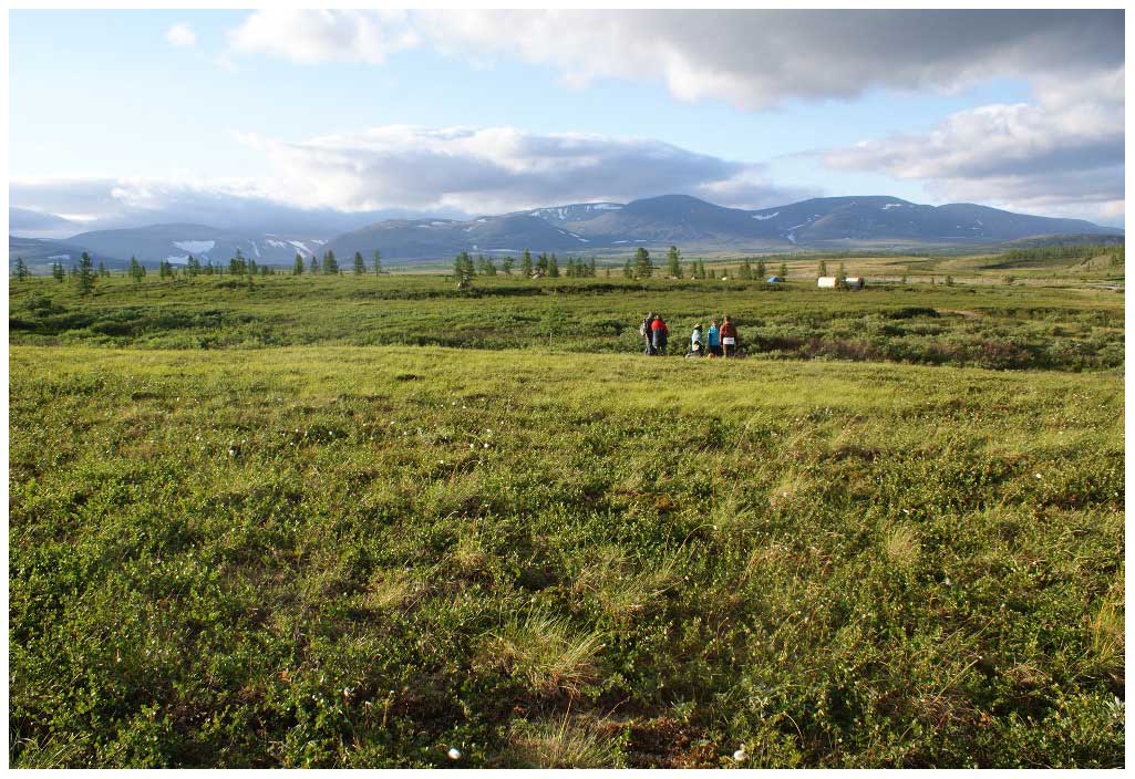
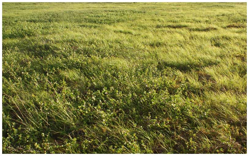
Figure B13 Example photograph CALU no. 5 (Elena Troeva, 2017; northern Yamal).

B6 CALU no. 6

Description. Dry to moist tundra, partially barren, prostrate shrubs, medium organic layer thickness, high mineral volumetric content.

Figure B14 CALU no. 6 vegetation properties based on AVA (Zemlianskii et al., 2023).

Figure B15 CALU no. 6 soil properties based on Palmtag et al. (2022).

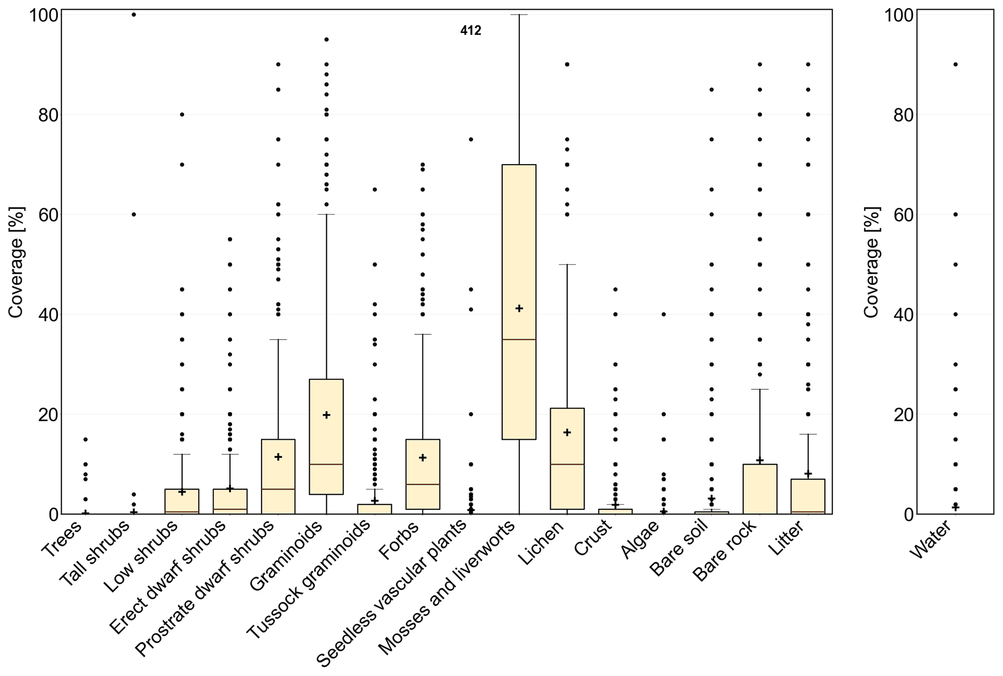
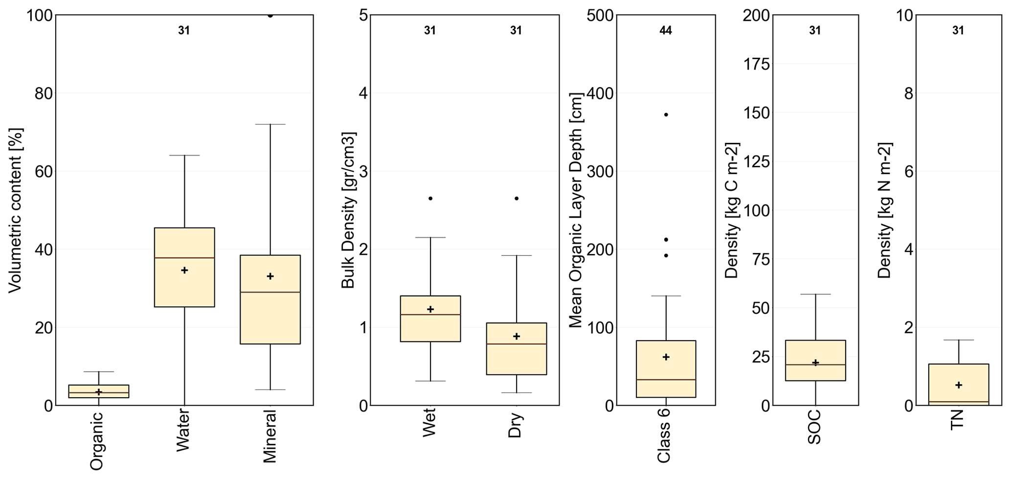
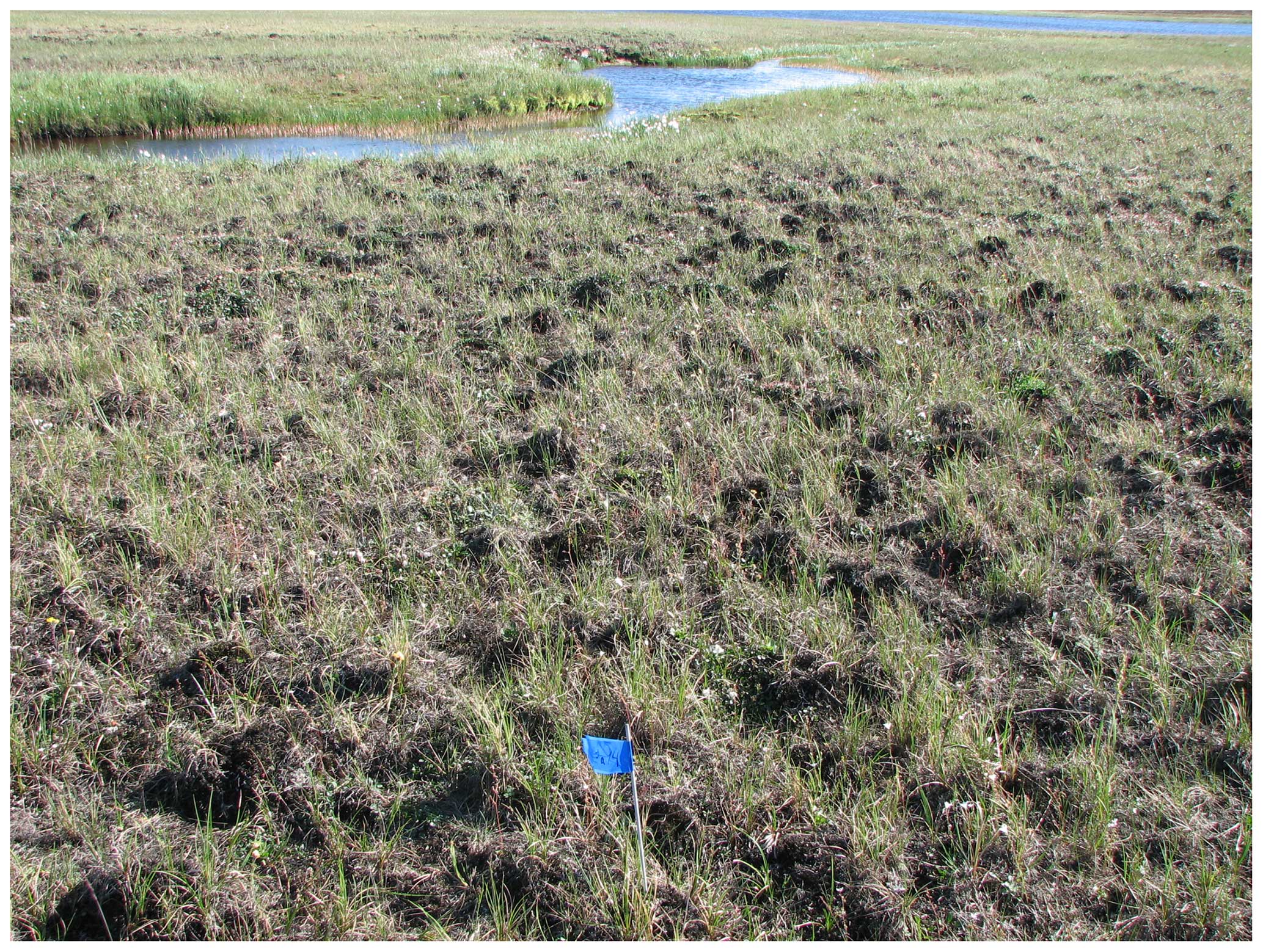
Figure B16 Example photograph CALU no. 6, foreground (Elena Troeva, 2017; northern Yamal).

B7 CALU no. 7

Description. Dry tundra, abundant lichen, prostrate shrubs, low to medium organic layer thickness, high mineral volumetric content.

Figure B17 CALU no. 7 vegetation properties based on AVA (Zemlianskii et al., 2023).

Figure B18 CALU no. 7 soil properties based on Palmtag et al. (2022).

Figure B19 Example photograph CALU no. 7 (Annett Bartsch 2018; Polar Urals).

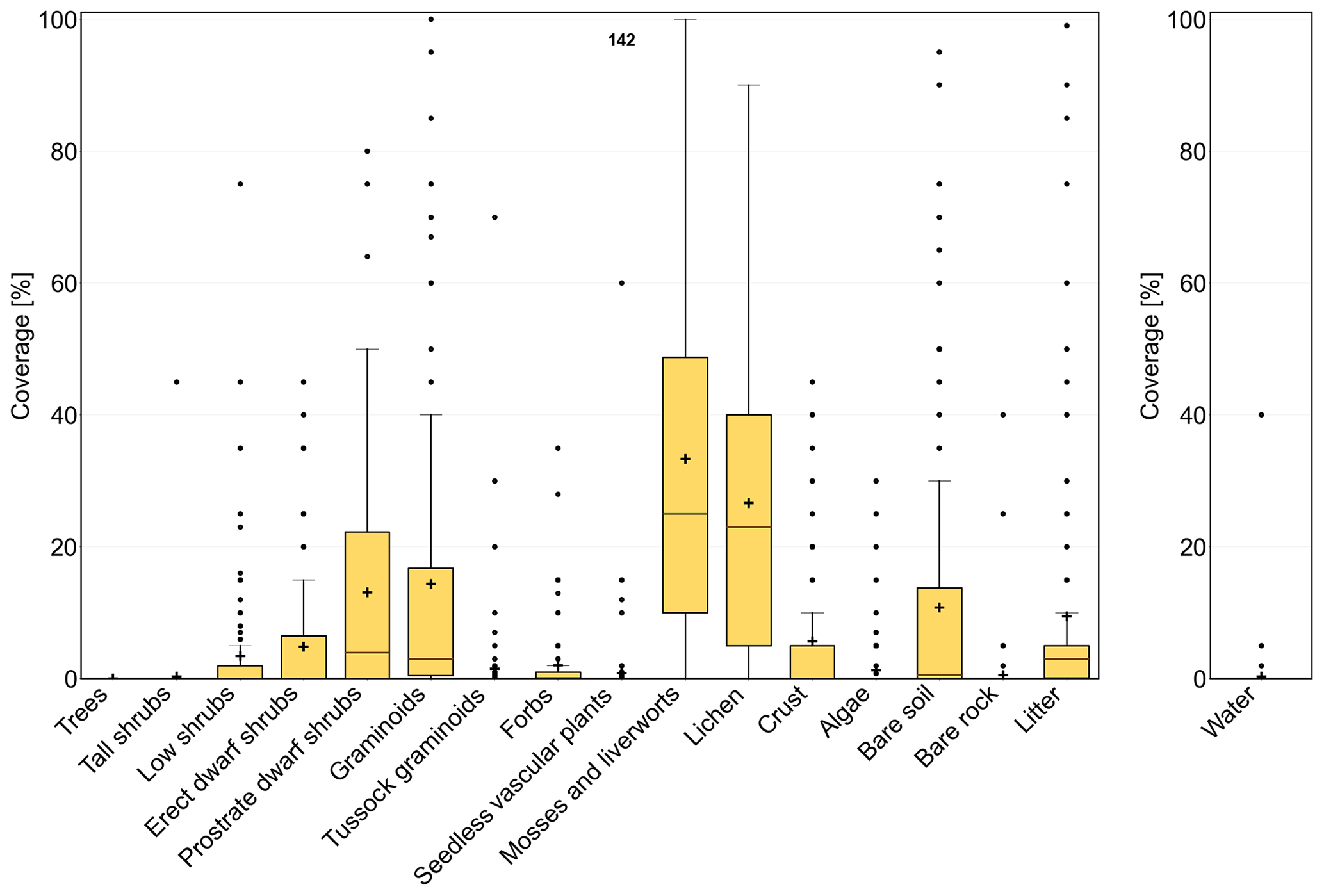
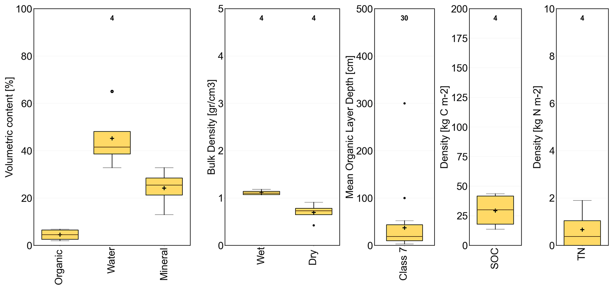
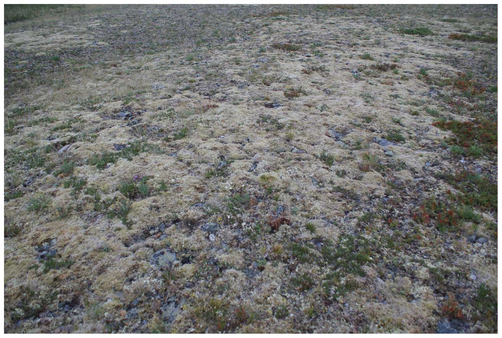
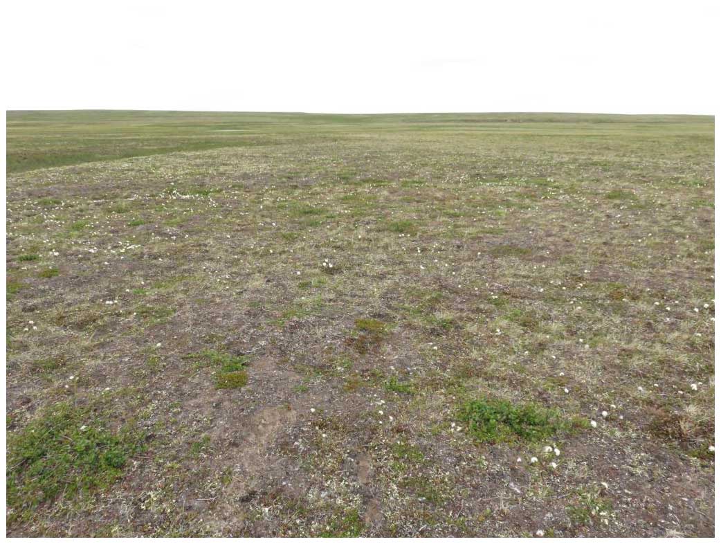
Figure B20 Example photograph CALU no. 7 (Olga Khitun, 2017; central Gydan).

B8 CALU no. 8

Description. Dry to aquatic tundra, dwarf shrubs (sparse tree cover along treeline, woodlands and open stands), medium organic layer thickness, medium mineral volumetric content.

Figure B21 CALU no. 8 vegetation properties based on AVA (Zemlianskii et al., 2023).

Figure B22 CALU no. 8 soil properties based on Palmtag et al. (2022).

Figure B23 Example photograph CALU no. 8 (Birgit Heim, 2019, Samoylov, Lena Delta).

Figure B24 Example photograph CALU no. 8 (Annett Bartsch, 27 July 2023; Inuvik region).

B9 CALU no. 9

Description. Dry to moist tundra, prostrate to low shrubs, tussocks, low to medium organic layer thickness, medium mineral volumetric content.

Figure B25 CALU no. 9 vegetation properties based on AVA (Zemlianskii et al., 2023).

Figure B26 CALU no. 9 soil properties based on Palmtag et al. (2022).

Figure B27 Example photograph CALU no. 9 (Marina Leibman, 29 August 2014; central Yamal).

Figure B28 Example photograph CALU no. 9 (Annett Bartsch, 21 July 2023; Inuvik region).

Figure B29 Example photograph CALU no. 9 (Birgit Heim, 2018; Lena Delta, third terrace).

B10 CALU no. 10

Description. Moist tundra, abundant moss, prostrate to low shrubs, tussocks, low organic layer thickness, medium mineral volumetric content.

Figure B30 CALU no. 10 vegetation properties based on AVA (Zemlianskii et al., 2023).

Figure B31 CALU no. 10 soil properties based on Palmtag et al. (2022).

Figure B32 Example photograph CALU no. 10 (Marina Leibman, 2014; central Yamal).

B11 CALU no. 11

Description. Moist tundra, abundant moss, dwarf and low shrubs, tussocks, low organic layer thickness, medium mineral volumetric content.

Figure B33 CALU no. 11 vegetation properties based on AVA (Zemlianskii et al., 2023).

Figure B34 CALU no. 11 soil properties based on Palmtag et al. (2022).

Figure B35 Example photograph CALU no. 11 (Annett Bartsch, 28 July 2018; Polar Urals).

Figure B36 Example photograph CALU no. 11 (Annett Bartsch, 19 July 2023; Inuvik region).

B12 CALU no. 12

Description. Moist tundra, dense dwarf and low shrubs (sparse tree cover along treeline, woodlands with open stands), medium organic layer thickness, low mineral volumetric content.

Figure B37 CALU no. 12 vegetation properties based on AVA (Zemlianskii et al., 2023).

Figure B38 CALU no. 12 soil properties based on Palmtag et al. (2022).

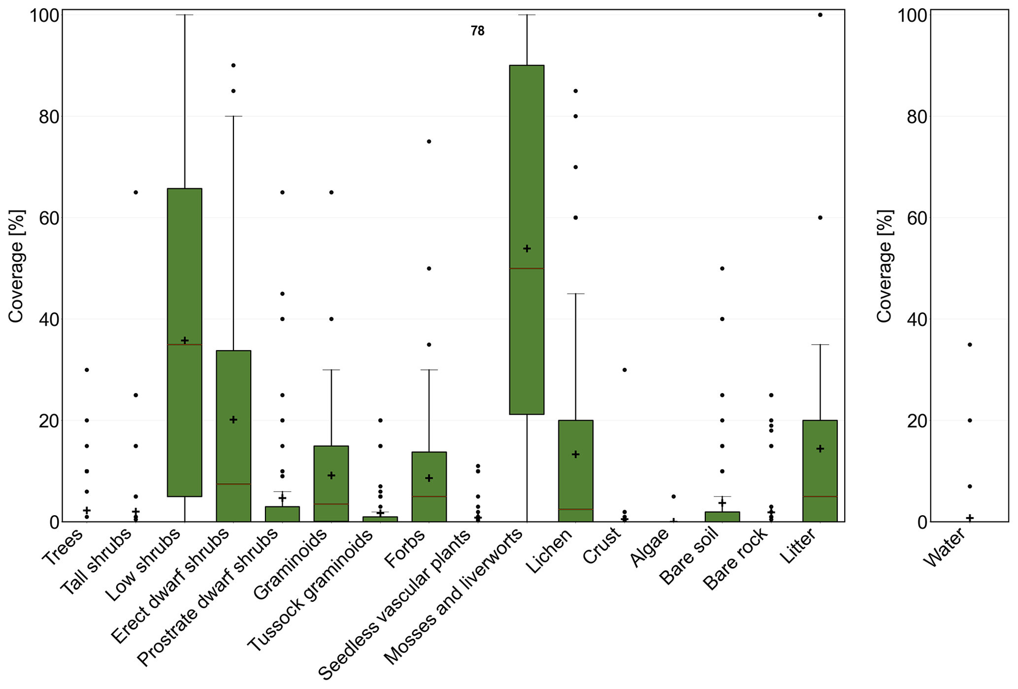
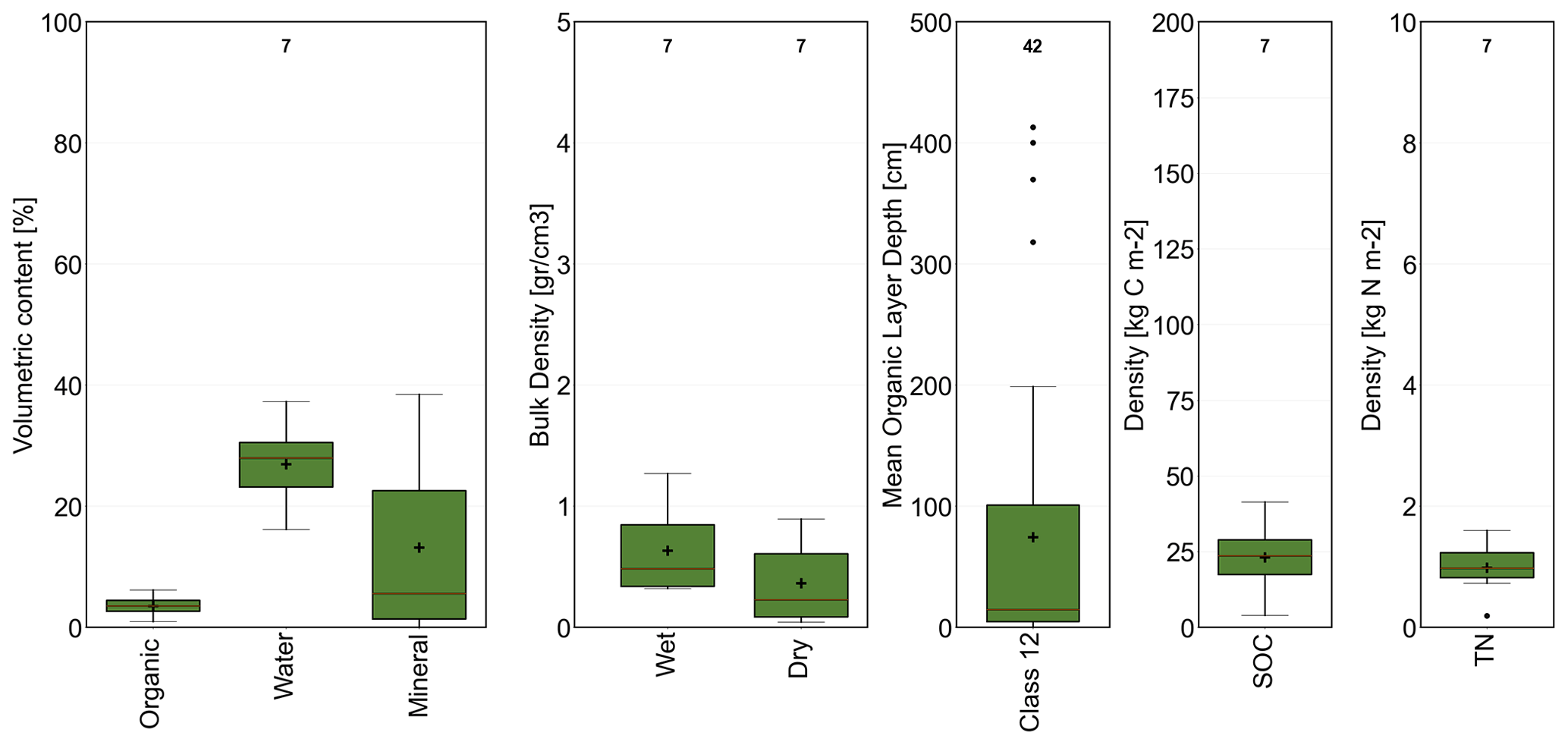
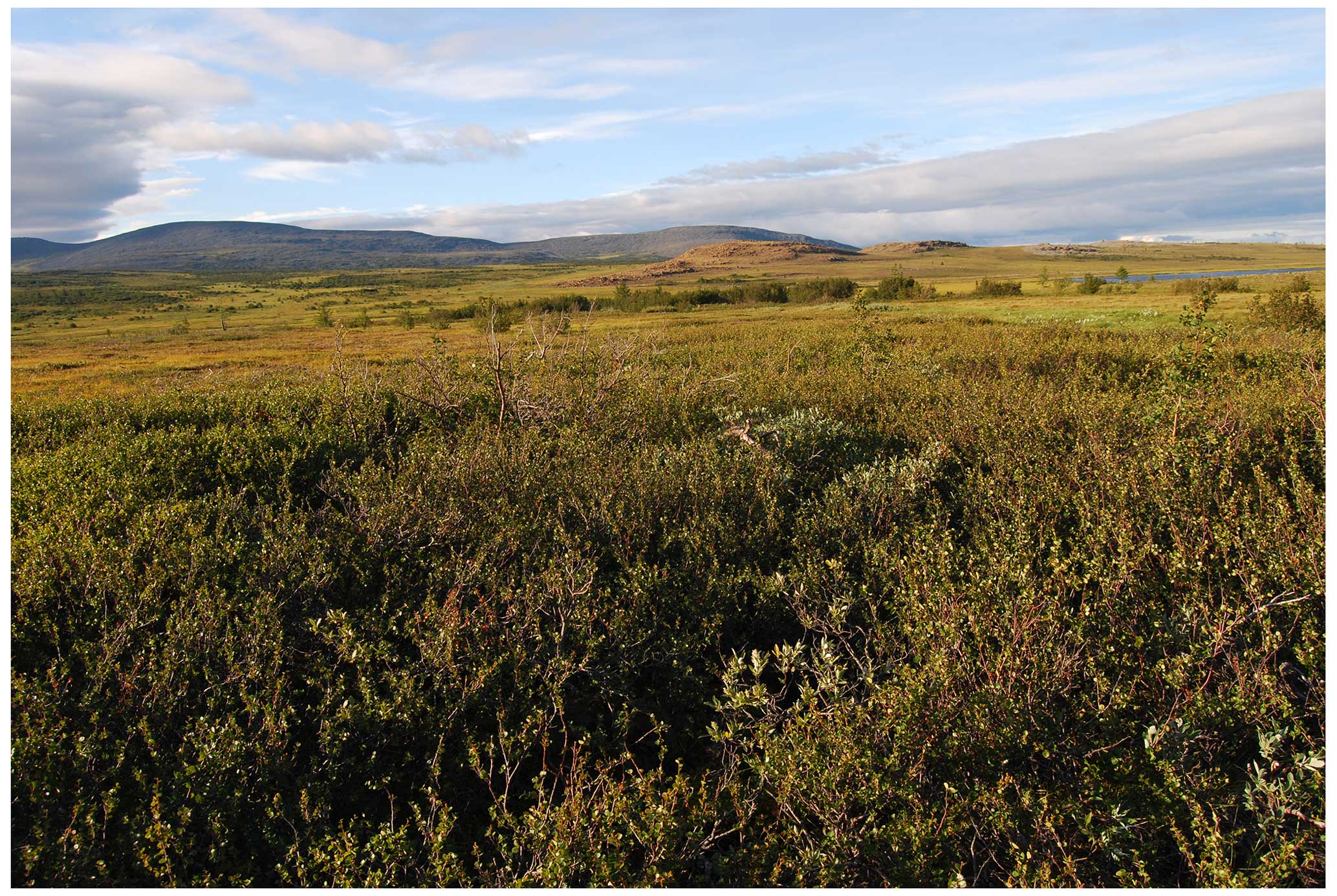
Figure B39 Example photograph CALU no. 12, foreground (Ksenia Ermokhina, 1 August 2011; Polar Urals, mostly Betula nana, scattered Salix ssp.).

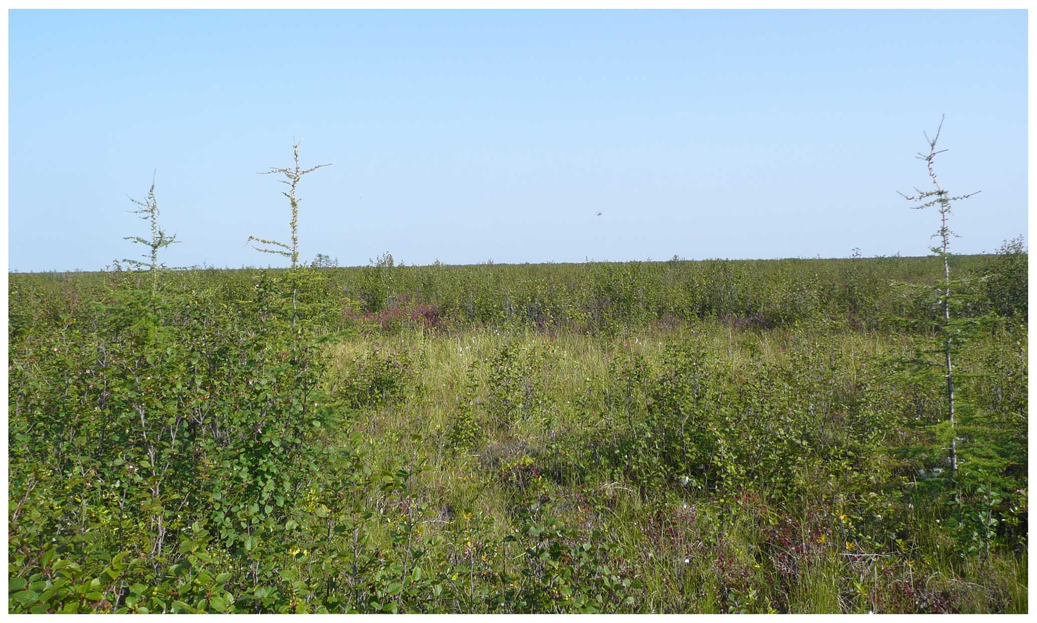
Figure B40 Example photograph CALU no. 12 (Mareike Wieczorek, 11 August 2012; Kolyma region, mostly Betula nana in proximity to patches of CALU no. 3.

B13 CALU no. 13

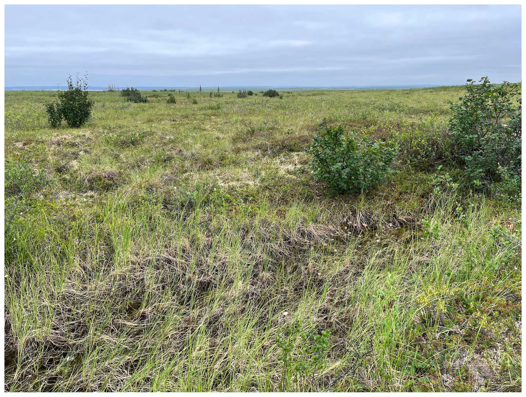
Description. Moist to wet tundra, dense dwarf and low shrubs (sparse tree cover along treeline, woodlands with open stands).

Figure B41 CALU no. 13 vegetation properties based on AVA (Zemlianskii et al., 2023).

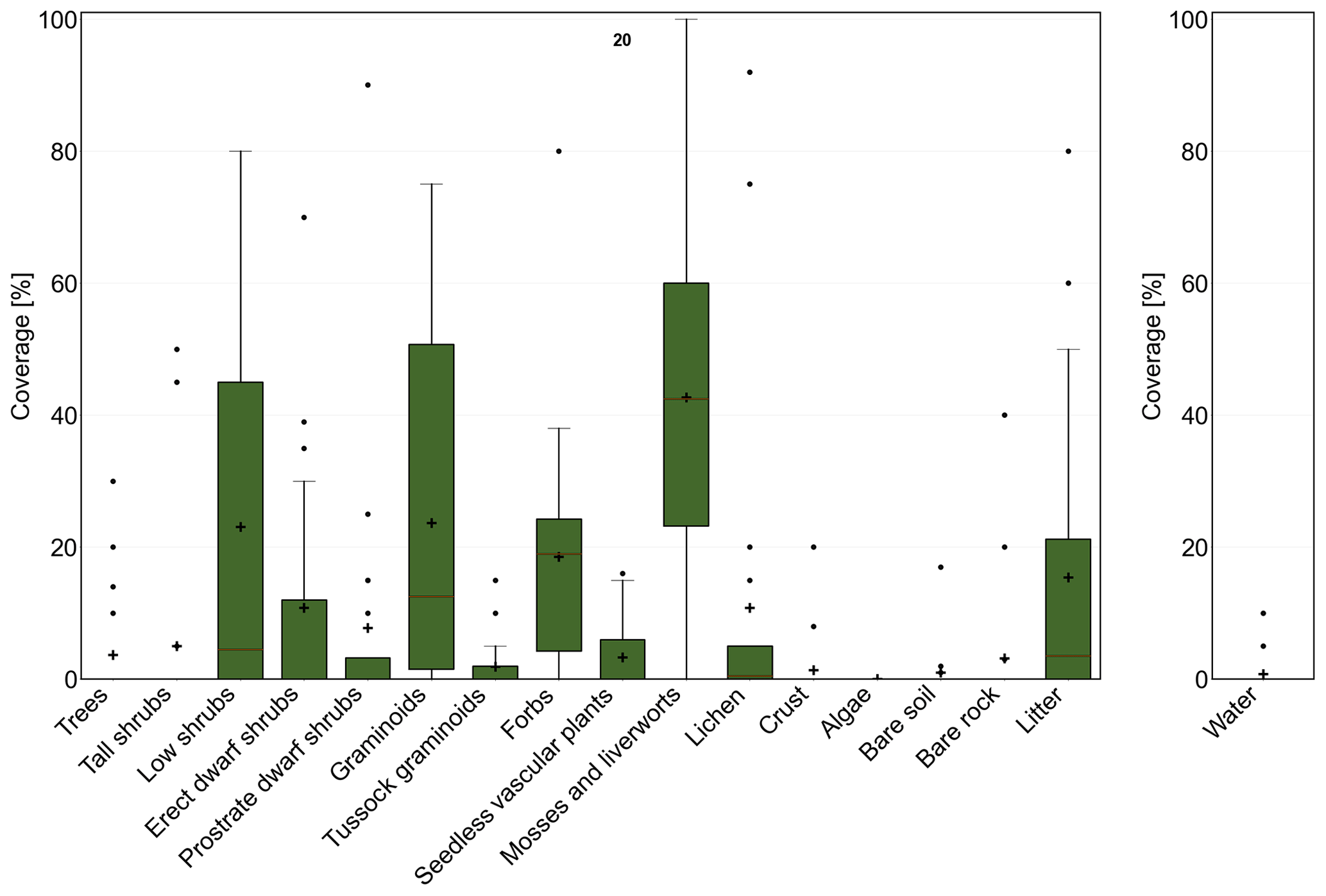
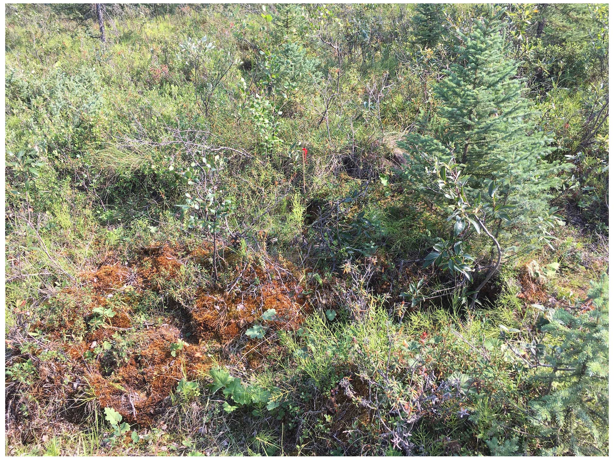
Figure B42 Example photograph CALU no. 13 (Clemens von Baeckmann, 25 July 2023; Inuvik region).

B14 CALU no. 14

Description. Moist tundra, low shrubs, medium organic layer thickness, medium mineral volumetric content.

Figure B43 CALU no. 14 vegetation properties based on AVA (Zemlianskii et al., 2023).

Figure B44 CALU no. 14 soil properties based on Palmtag et al. (2022).

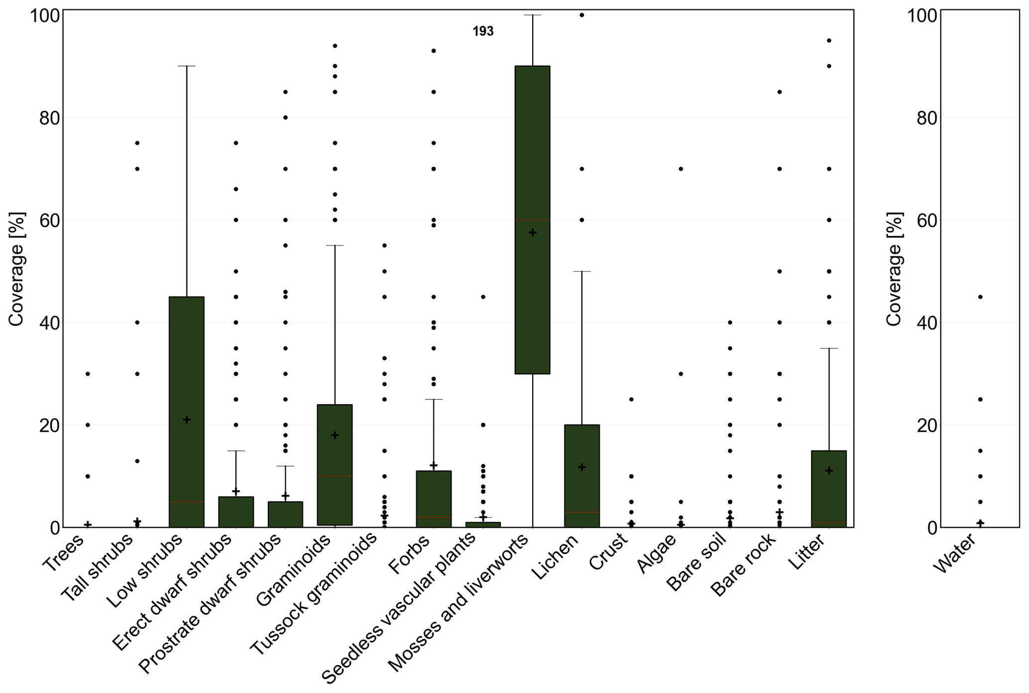
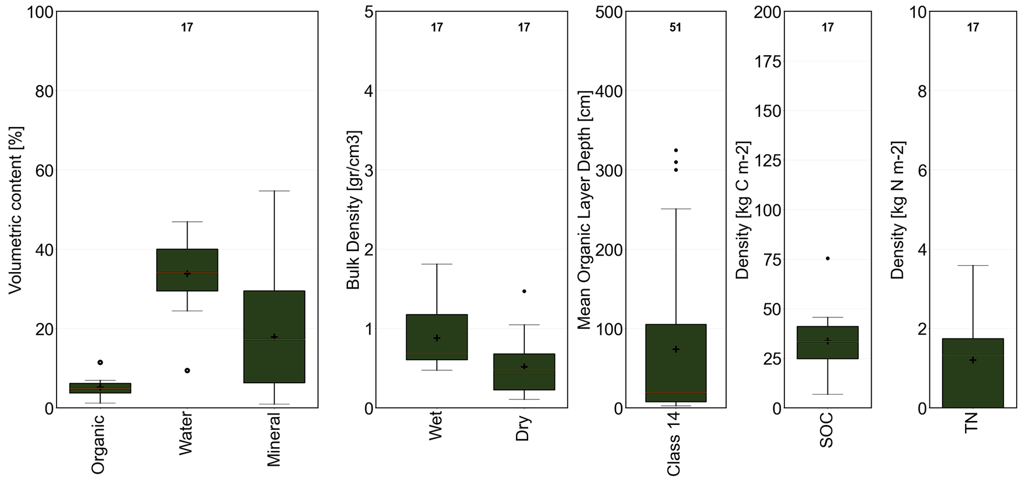
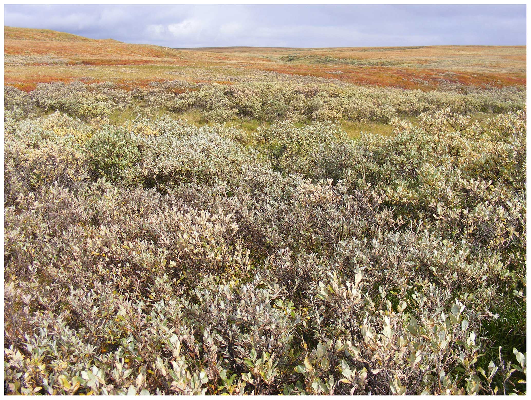
Figure B45 Example photograph CALU no. 14 (Marina Leibman, 29 August 2014; central Yamal, mostly Salix ssp.).

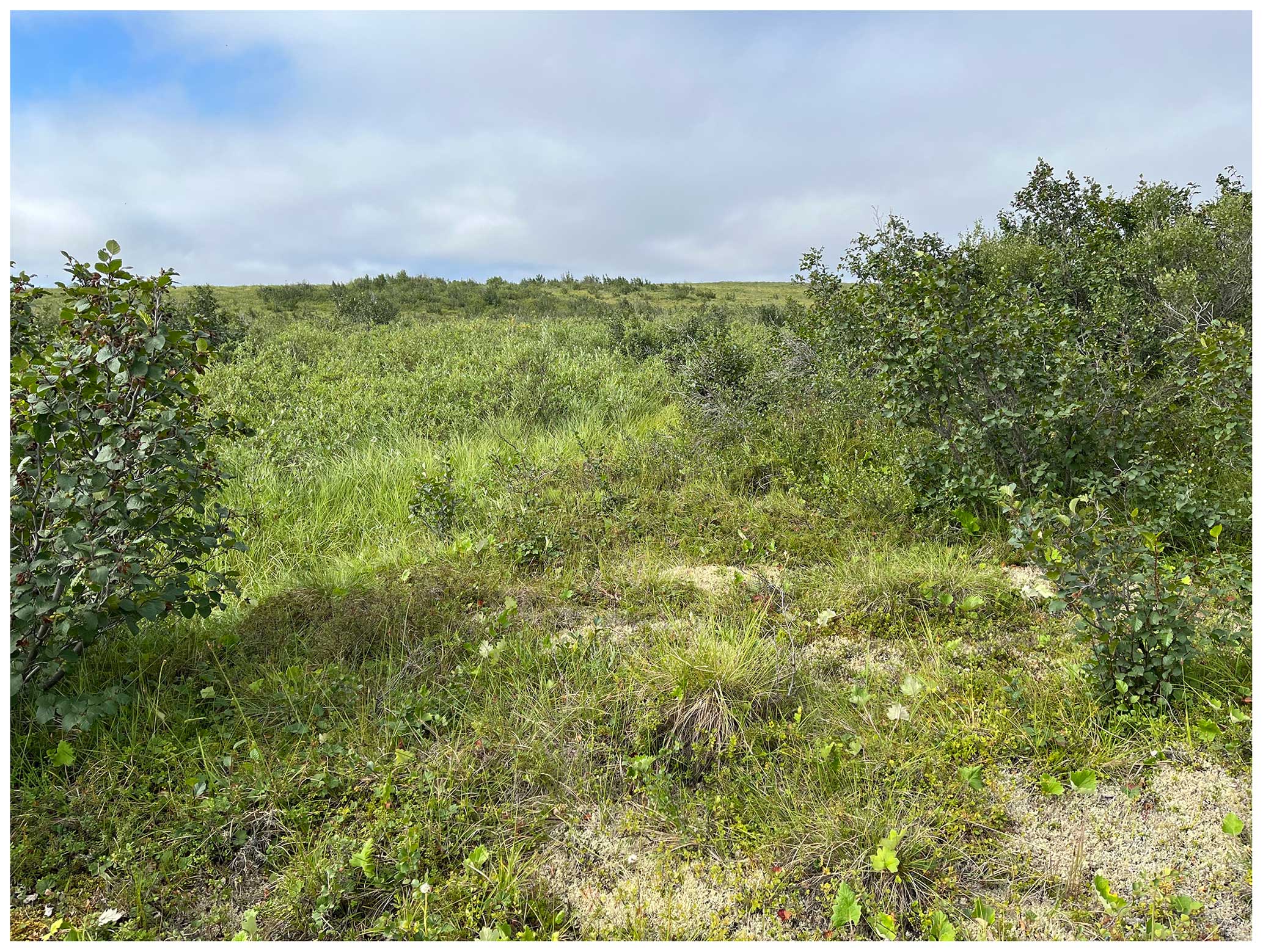
Figure B46 Example photograph CALU no. 14 (Annett Bartsch, 24 July 2023; Inuvik region, background Salix ssp., left and right Alnus ssp.).

B15 CALU no. 15

Description. Moist to wet tundra, abundant lichen, in some cases partially barren (disturbed).

Figure B47 CALU no. 15 vegetation properties based on AVA (Zemlianskii et al., 2023).

Figure B48 CALU no. 15 soil properties based on Palmtag et al. (2022).

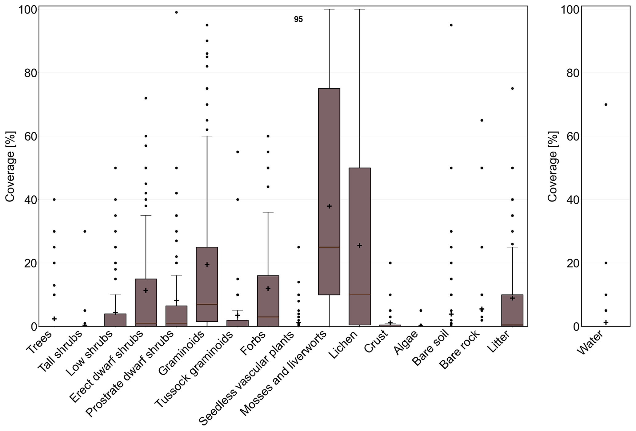
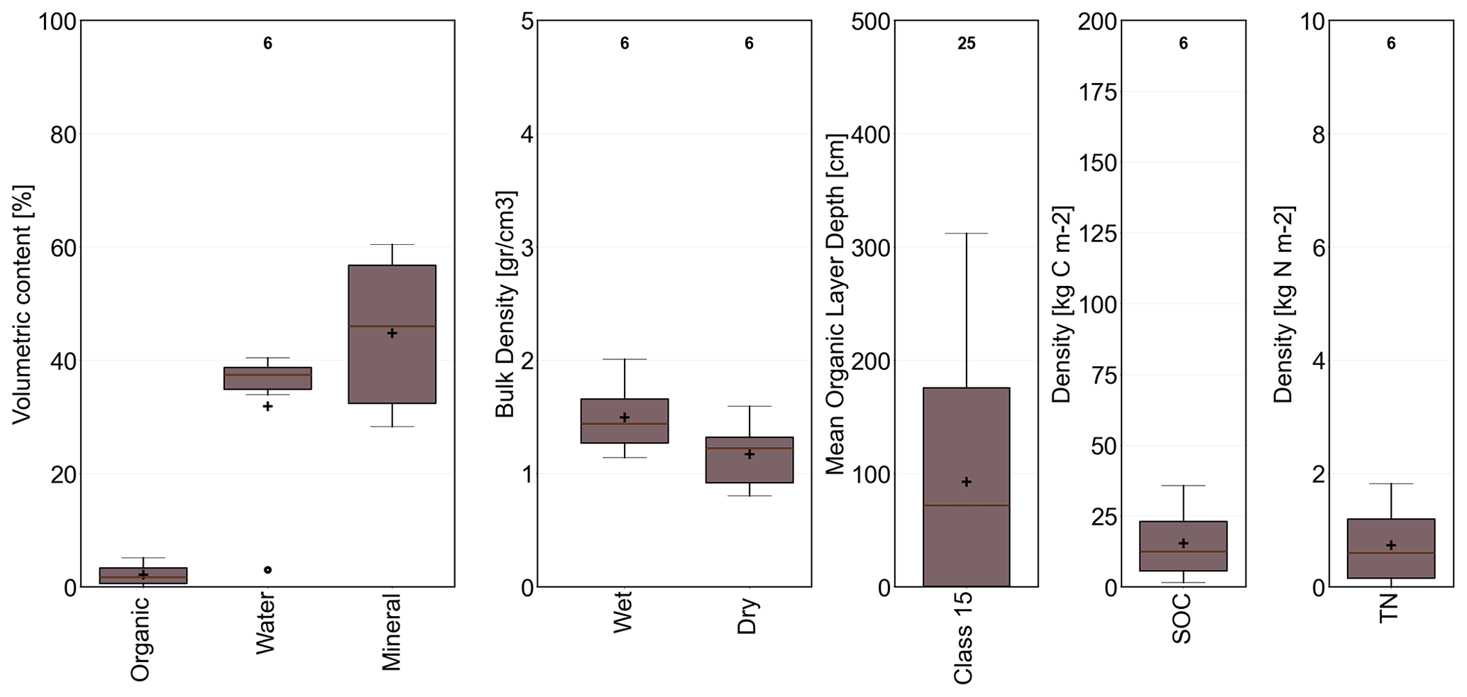
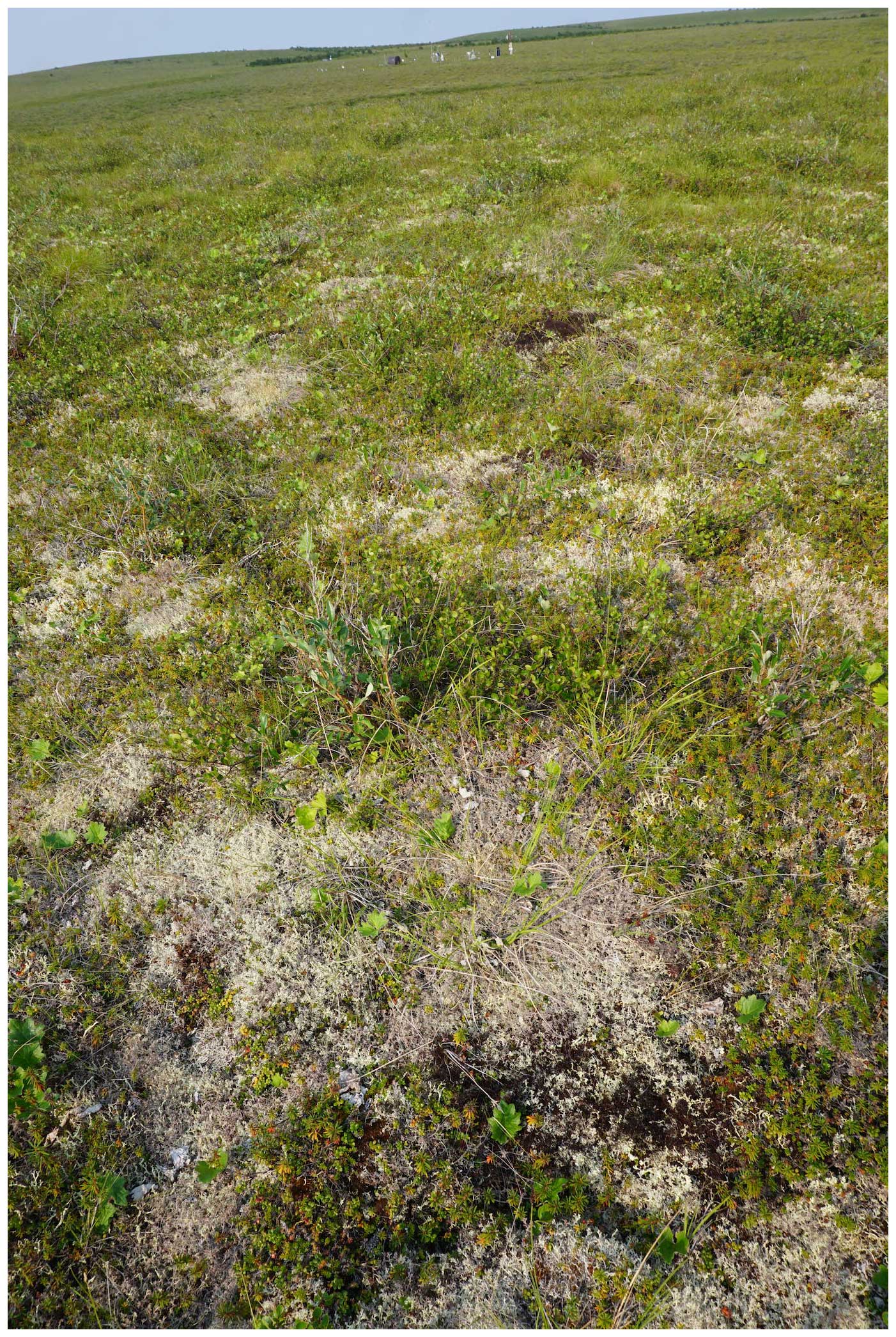
Figure B49 Example photograph CALU no. 15 (Veronika Döpper, 17 July 2023; Inuvik region).

B16 CALU no. 16

Description. Moist tundra, abundant forbs, dwarf to tall shrubs, medium organic layer thickness.

Figure B50 CALU no. 16 vegetation properties based on AVA (Zemlianskii et al., 2023).

Figure B51 CALU no. 16 soil properties based on Palmtag et al. (2022).

Figure B52 Example photograph CALU no. 16 (Annett Bartsch, 28 July 2018; Polar Urals).

B17 CALU no. 17

Description. Recently burned or flooded, partially barren.

Figure B53 CALU no. 17 vegetation properties based on AVA (Zemlianskii et al., 2023).

Figure B54 Example photograph CALU no. 17 (Annett Bartsch, 27 July 2023; Inuvik region).

B18 CALU no. 18

Description. Forest (deciduous) with dwarf to tall shrubs.

Figure B55 CALU no. 18 vegetation properties based on AVA (Zemlianskii et al., 2023).

B19 CALU no. 19

Description. Forest (mixed) with dwarf to tall shrubs.

Figure B56 CALU no. 19 vegetation properties based on AVA (Zemlianskii et al., 2023).

Figure B57 CALU no. 19 soil properties based on Palmtag et al. (2022).

B20 CALU no. 20

Description. Forest (needle leaf) with dwarf and low shrubs.

Figure B58 CALU no. 20 vegetation properties based on AVA (Zemlianskii et al., 2023).

Figure B59 CALU no. 20 soil properties based on Palmtag et al. (2022).

B21 CALU no. 21

Description. Partially barren, dry.

Figure B60 CALU no. 21 vegetation properties based on AVA (Zemlianskii et al., 2023).

Figure B61 CALU no. 21 soil properties based on Palmtag et al. (2022).

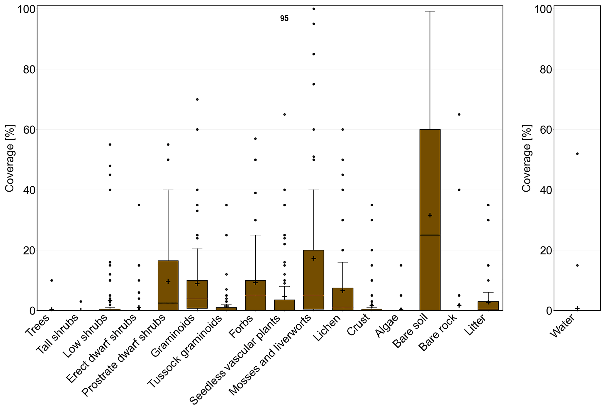
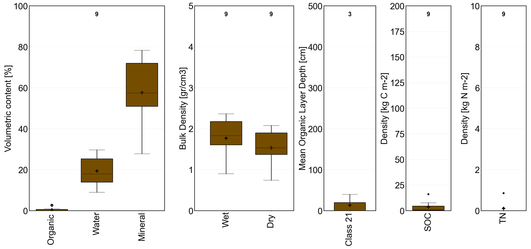
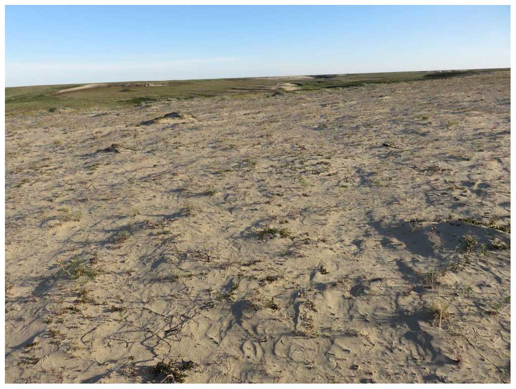
Figure B62 Example photograph CALU no. 21 (Olga Khitun, 2017; Tazovskiy Peninsula).

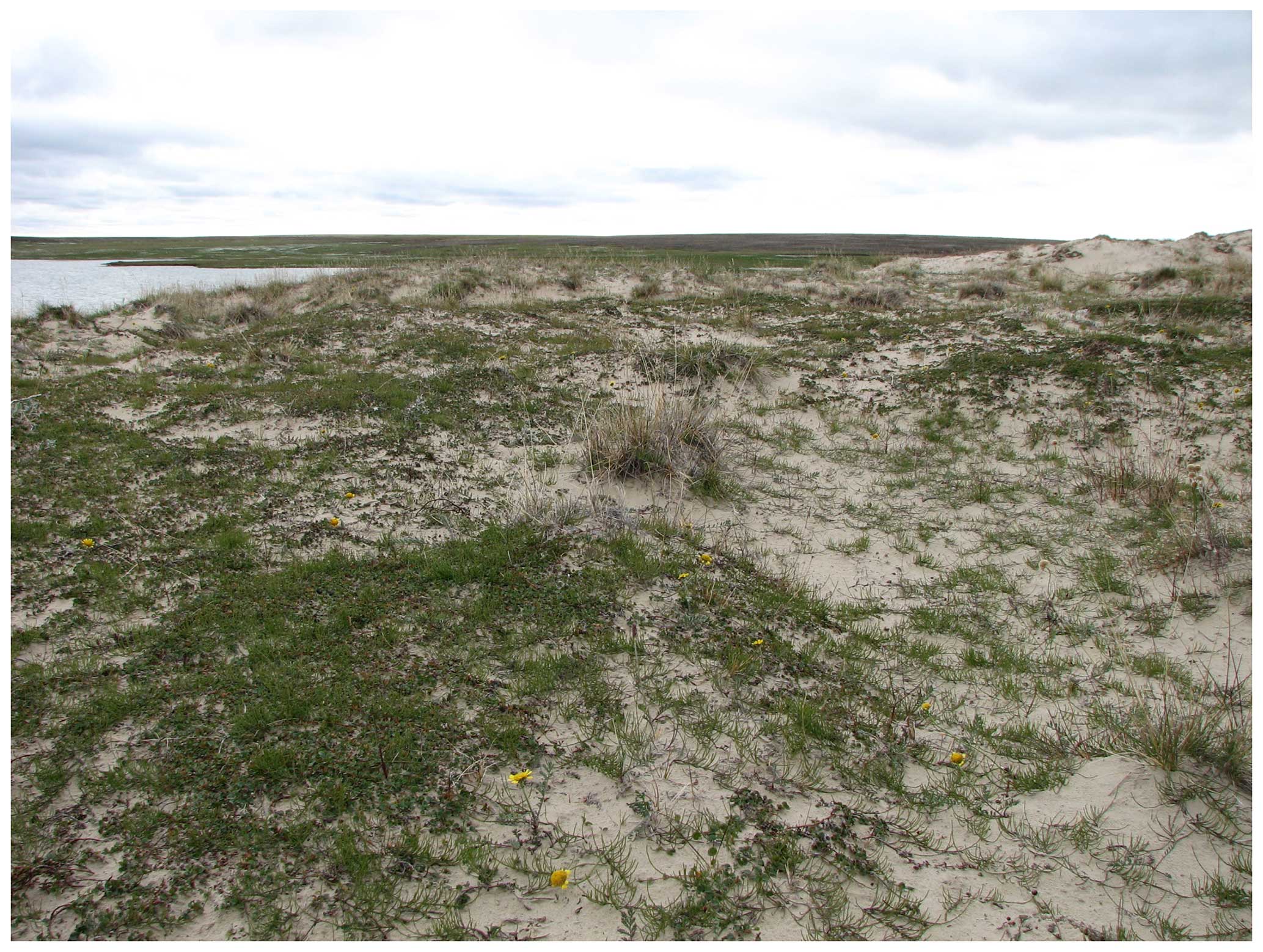
Figure B63 Example photograph CALU no. 21 (Elena Troeva, 2017; northern Yamal).

Appendix C: Comparison schemes and matrices for external land cover datasets

Table C1 Classes of ESA CCI Land Cover (http://maps.elie.ucl.ac.be/CCI/viewer/index.php, last access: 1 September 2023) and grouping for comparison (see Table 2).

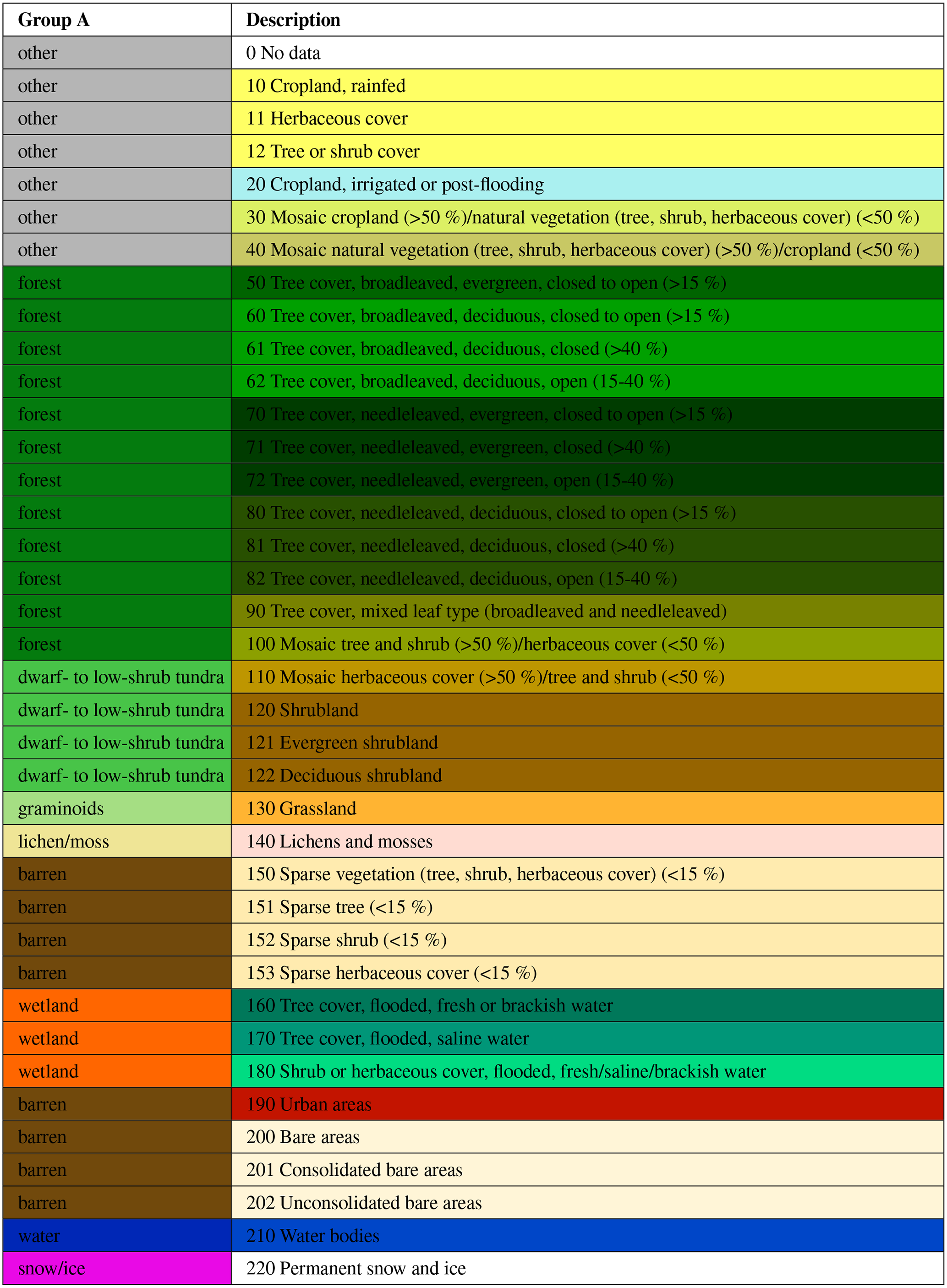
Table C2 Classes of the CAVM (Raynolds et al., 2019) and grouping for comparison (see Table 2).

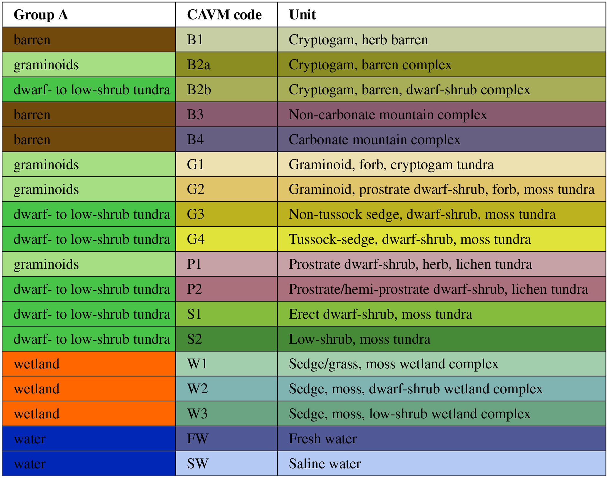
Table C3 Classes of the CALC-2020 (Liu et al., 2023) and grouping for comparison (see Table 2).

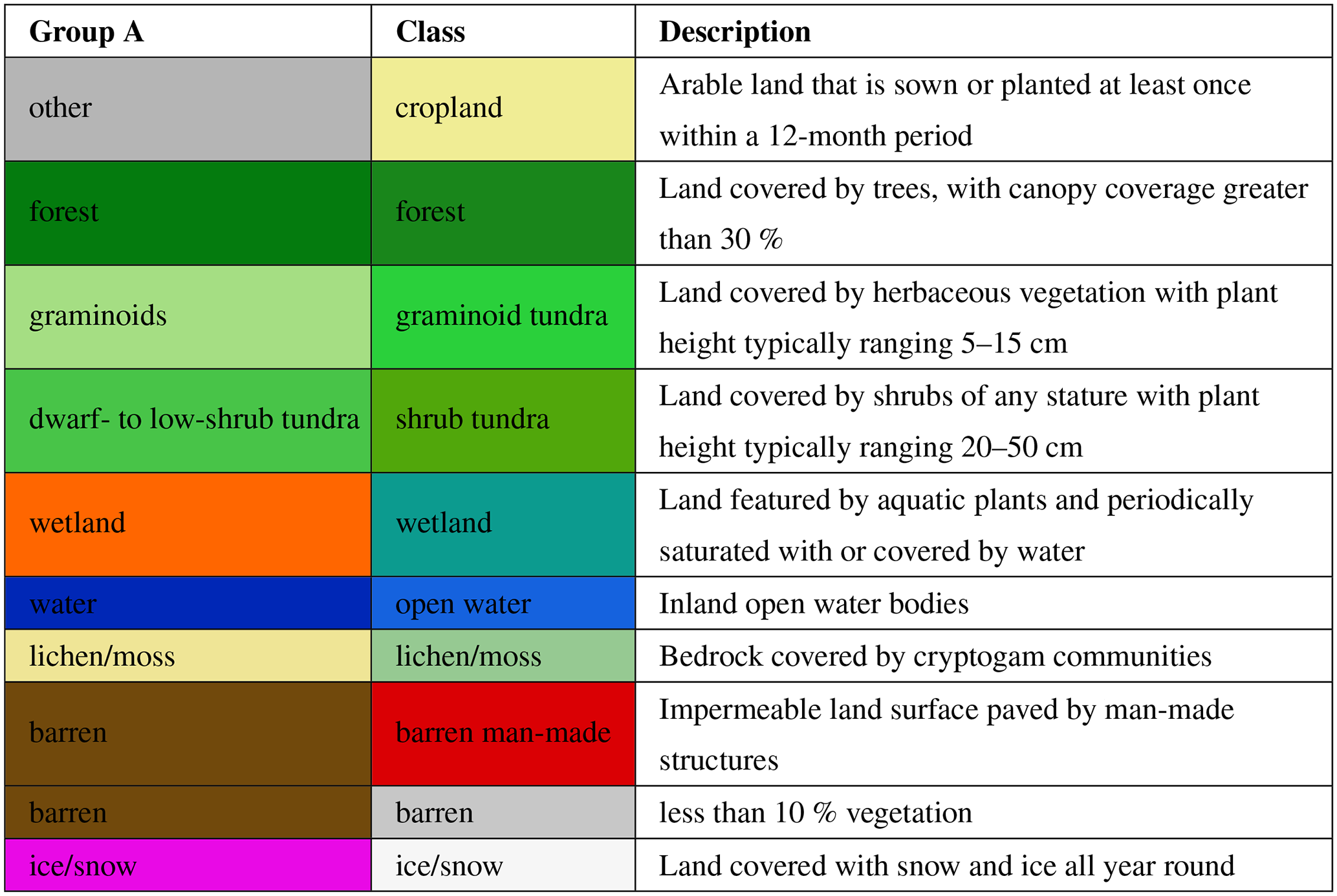
Table C4 Comparison matrix of grouped Circumpolar Arctic Vegetation Map (CAVM) classes and grouped units (Circumarctic Land cover Units – CALU). Values in percent. For grouping schemes, see Tables 2 and C2.

Table C5 Comparison matrix of grouped circumpolar Arctic land cover (CALC-2020) land cover classes and grouped units (Circumarctic Land cover Units – CALU). Values in percent. For grouping schemes, see Table 2 and Table C3.

Appendix D: Changes between prototype and CALU

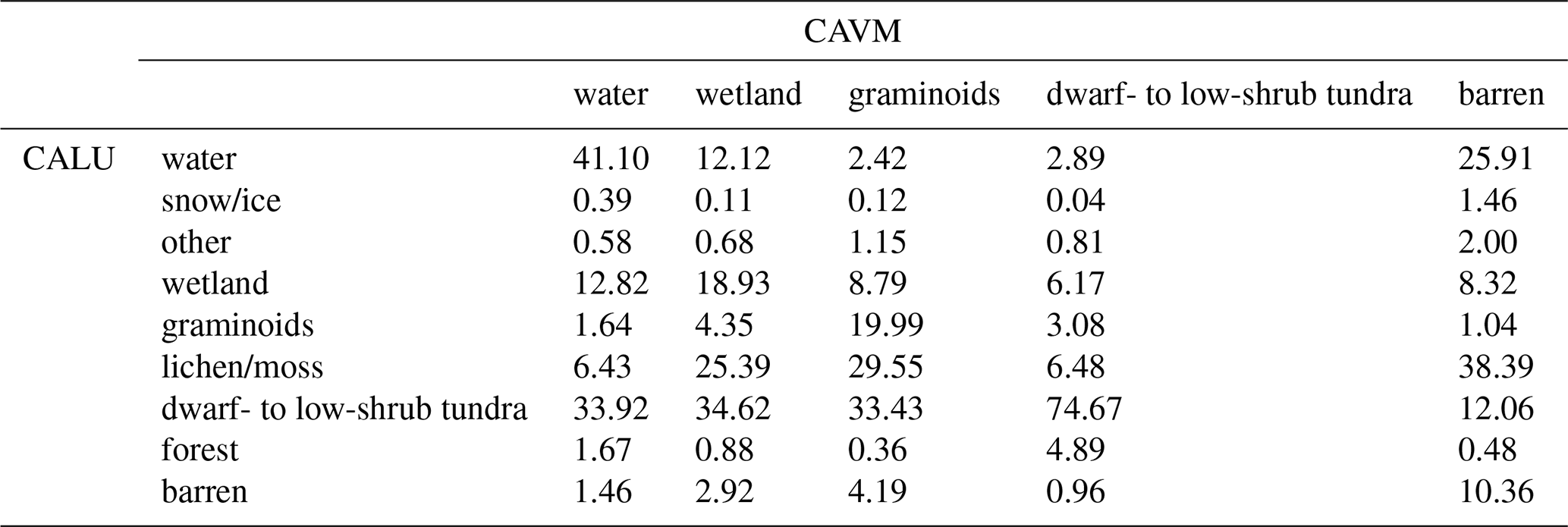
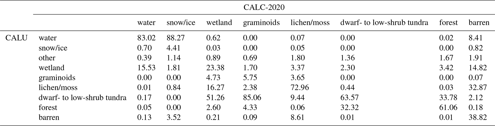
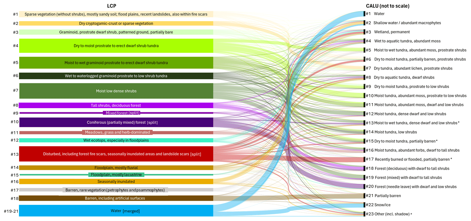
Figure D1 Visualization of changed mapping units from the land cover prototype (LCP; 20 m) to CALU (10 m). The three water classes of the LCP are merged. New units are marked with ^*.