Differentiating between crop and soil effects on soil moisture dynamics

There is an urgent need to develop sustainable agricultural land use schemes. Intensive crop production has induced increased greenhouse gas emissions and enhanced nutrient and pesticide leaching to groundwater and streams. Climate change is also expected to increase drought risk as well as the frequency of extreme precipitation events in many regions. Consequently, sustainable management schemes require sound knowledge of site-specific soil water processes that explicitly take into account the interplay between soil heterogeneities and crops. In this study, we applied a principal component analysis to a set of 64 soil moisture time series from a diversified cropping field featuring seven distinct crops and two weeding management strategies.

Results showed that about 97 % of the spatial and temporal variance of the data set was explained by the first five principal components. Meteorological drivers accounted for 72.3 % of the variance and 17.0 % was attributed to different seasonal behaviour of different crops. While the third (4.1 %) and fourth (2.2 %) principal components were interpreted as effects of soil texture and cropping schemes on soil moisture variance, respectively, the effect of soil depth was represented by the fifth component (1.7 %). However, neither topography nor weed control had a significant effect on soil moisture variance. Contrary to common expectations, soil and rooting pattern heterogeneity seemed not to play a major role. Findings of this study highly depend on local conditions. However, we consider the presented approach generally applicable to a large range of site conditions.

1 Introduction

Agriculture plays a major role in ensuring the provision of food to a growing global population. At the same time, climate change is putting yield stability at risk due to extreme weather events, increasing the need for sustainable management of resources such as water and soil (Trnka et al., 2014). The transformation from large homogeneously cropped fields towards diversified agricultural landscapes has been identified as an opportunity that can contribute to climate adaptation due to the positive effects on multiple ecosystem services (Tamburini et al., 2020) and cropping system resilience to climatic extremes (Birthal and Hazrana, 2019). Additionally, crop diversification is highly beneficial by reducing soil erosion through permanent soil cover (Paroda et al., 2015) and by improving resource use efficiency through wider crop rotations (Rodriguez et al., 2021).

In terms of soil water dynamics, crop and management diversification can lead to improved water-stable macro-aggregation, reduced soil compaction, and increased soil organic carbon, which can reduce soil water infiltration and improve water retention (Alhameid et al., 2020; Fischer et al., 2014; Karlen et al., 2006; Koudahe et al., 2022; Nunes et al., 2018). Korres et al. (2015) reported that spatial variability in soil moisture was mainly driven by soil characteristics, followed by crop cover and management. Soil moisture is also affected by soil texture and pore size distribution (Krauss et al., 2010; Rossini et al., 2021; Pan and Peters-Lidard, 2008). The quantification of the impact of these effects on soil moisture variability is important, for instance for hydrological applications and adopted management practices in agriculture (Hupet and Vanclooster, 2002).

As the diversity of independent variables in agricultural systems increases, demands for frequency and spacing of soil moisture measurements and related data interpretation grow. Therefore, soil sensor networks are receiving increased attention, particularly in precision agriculture (PA; Bogena et al., 2022; Salam and Raza, 2020), where the main goal is to increase efficiency and productivity at the farm level while minimizing the negative impacts on the environment (Taylor and Whelan, 2010). Soil sensor networks can meaningfully contribute to PA as they can be used for various purposes, including the delineation of management zones (Khan et al., 2020; Salam and Raza, 2020). Still, one of the most important demands to be fulfilled by soil sensor networks is soil moisture monitoring, as accurate measurement of soil water content can play an important role in improving water management and, therefore, crop yields (Salam, 2020).

Wireless solutions, for instance based on long-range wide-area network (LoRaWAN) technology, in combination with electromagnetic soil moisture sensors avoid labour-intensive and destructive soil moisture measurements that disrupt field traffic. The development of such wireless sensor networks (WSNs) enables broad and affordable application also in areas with low cellular coverage (Cardell-Oliver et al., 2019; Lloret et al., 2021; Placidi et al., 2021; Prakosa et al., 2021).

The evolution of WSN not only has benefits for management but is also of high relevance for fostering the understanding of hydrological dynamics in the vadose zone. High-resolution data sets measured under real farming conditions can be used to characterize and analyse spatiotemporal dynamics of soil water. Due to the large size of data sets that are recorded with WSN, sophisticated data analysis approaches are required to detect hidden patterns and determine influence factors on soil moisture variability (Vereecken et al., 2014). With the introduction of multiple-point geostatistics it became possible to not only analyse patterns but also connect them with factors affecting soil moisture, such as topography, texture, crop growth and water uptake, and land management (Brocca et al., 2010; Strebelle et al., 2003). Wavelet analysis can analyse both localized features and spatial trends through which non-stationary variation in soil properties can be considered (Si, 2008). Cross-correlation analysis allows linking soil moisture variability to climatic variables (Mahmood et al., 2012). Furthermore, temporal stability analyses detect spots in the investigated area which are consistently wetter or drier than the mean soil moisture (Baroni et al., 2013; Vachaud et al., 1985, Vanderlinden et al., 2012). This method was already successfully used to detect soil moisture patterns related to soil properties, vegetation, and topography (Zhao et al., 2010).

Principal component analysis (PCA) is another method that was successfully applied for soil moisture variability analysis at the field (Hohenbrink et al., 2016; Hohenbrink and Lischeid, 2015; Martini et al., 2017), catchment (Korres et al., 2010; Lischeid et al., 2017; Nied et al., 2013; Graf et al., 2014), and regional (Joshi and Mohanty, 2010) scales. These studies build on previous applications in climatology where the term “empirical orthogonal functions” is used (Bretherton et al., 1992) and are examples of how space and time dimensions can be disentangled and assigned to influencing factors. Additionally, the propagation of hydrological signals (e.g. precipitation events) over depth can be assessed (Hohenbrink et al., 2016). This presents great opportunities to improve the knowledge of changing soil water dynamics in complex diversified agricultural systems with increasing heterogeneity (e.g. soil texture) and site-specific adjustment of crop and field management, which, to our knowledge, have hardly been studied so far.

The main objective of this study was to identify the drivers of soil moisture variability in a diversified cropping field in terms of soil texture, crop selection, and field management by applying PCA. Special focus was put on the interpretation of spatial and temporal effects of crop diversification and of soil heterogeneities on soil moisture dynamics. For this, we analysed a high-resolution soil moisture data set measured by a novel underground LoRaWAN monitoring system with soil moisture sensors in different depths of the vadose zone at a spatiotemporally diversified agricultural field in northeastern Germany. The novelty of this WSN relies on its unique on-farm installation environment. The deployment of transmission units in 0.3 m soil depth and 180 sensors in up to 0.9 m soil depth allows high-spatiotemporal-resolution wireless data transmission and enables conventional farming practices like machinery traffic, tillage, and mechanical weeding.

2 Materials and methods

2.1 Study site

The study site (52°26^′51.8^′′ N, 14°08^′37.7^′′ E; 66–83 $\mathrm{m}\mathrm{a}.\mathrm{s}.\mathrm{l}.$) is located near the city of Müncheberg in the federal state of Brandenburg in northeastern Germany. The landscape is classified as a hummocky ground moraine that formed during the last glacial period. Glacial and interglacial processes, as well as subsequent erosion, resulted in highly heterogeneous soils (Deumlich et al., 2018) classified as Dystric Podzoluvisols according to the FAO scheme (Fischer et al., 2008). In the top 0.3 m soil layer, total organic carbon was 0.94 %, total nitrogen content was 0.07 %, and pH was 6.12. Between January 1991 and December 2020, the mean annual temperature in Müncheberg was 9.6 °C and the mean annual sum of precipitation was 509 mm (DWD Climate Data Center (CDC), 2021).

Table 1 Overview of crop rotation, sand content in the top 0.25 m soil depth, and weed control for selected patches at the patchCROP landscape experiment, Tempelberg, Brandenburg, Germany.

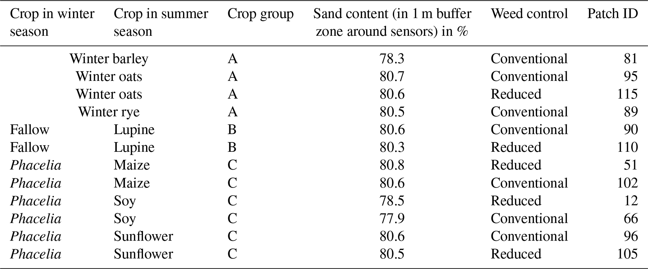
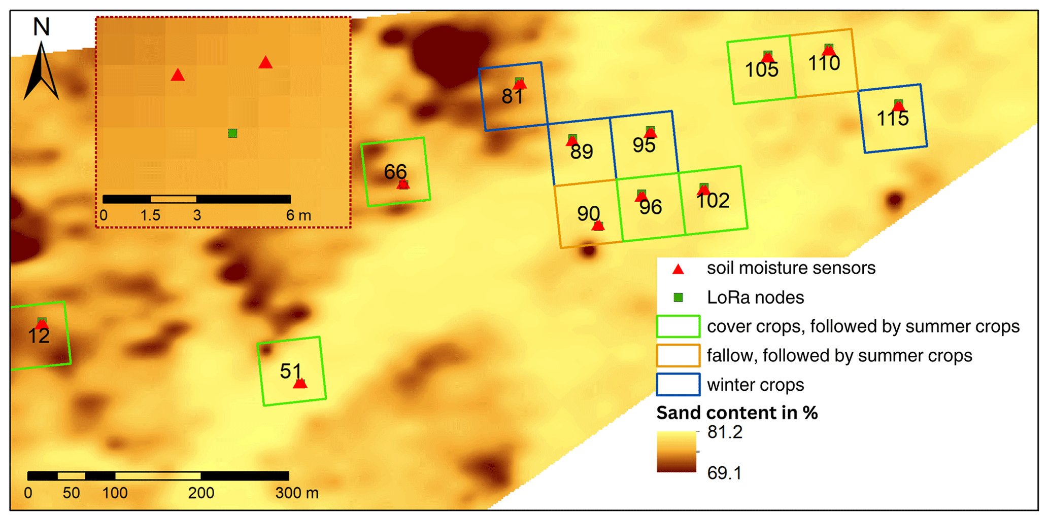
Figure 1 Sand content (in %) in the top 0.25 m soil depth, location of the analysed patches, soil moisture sensors (triangles), and LoRa nodes (squares) under different crop rotations at the patchCROP landscape experiment, Tempelberg, Brandenburg, Germany.

2.2 Experimental setup

The data collection was carried out from December 2020 until the middle of August 2021 in the patchCROP experiment (Grahmann et al., 2024; Donat et al., 2022). This landscape experiment has been set up to study the multiple effects of cropping system diversification on productivity, crop health, soil quality, and biodiversity. To that end, a cluster analysis was carried out based on soil maps and multi-year (2010–2019) yield data to identify high- and low-yield-potential zones in the 70 ha field (Donat et al., 2022). Afterwards, single experimental units comprising 30 patches with an individual size of 0.52 ha (72 × 72 m) each were implemented in both high- and low-yield-potential zones where each of those zones is characterized by varying soil conditions and a site-specific, 5-year, legume-based crop rotation (Grahmann et al., 2024). The remaining area outside of the 30 patches was planted with winter rye. For the current study, 12 out of 30 patches were considered (Fig. 1; Table 1). Specific patches were selected to capture the soil heterogeneities in terms of soil texture but also the seasonal patterns of the crop rotation that may have important effects on the soil water dynamics such as crop types, presence of cover crops, or fallow periods. In the cropping season 2020–2021, seven different main crops were grown. For subsequent data interpretation, crops have been grouped into (A) winter crops, (B) fallow followed by summer crops, and (C) cover crops followed by summer crops. In 7 out of 12 considered patches, weed control was carried out with herbicide application, referred to as “conventional” pesticide application, while in the remaining 5 patches, “reduced” pesticide management was carried out by mainly using mechanical weeding by harrowing, blind harrowing, and hoeing. Only in the case of high weed pressure were herbicides applied. Due to the potential impact of mechanical weeding, i.e. on rainwater infiltration, soil evaporation, and topsoil rooting intensity, we differentiate between these modes of weed control.

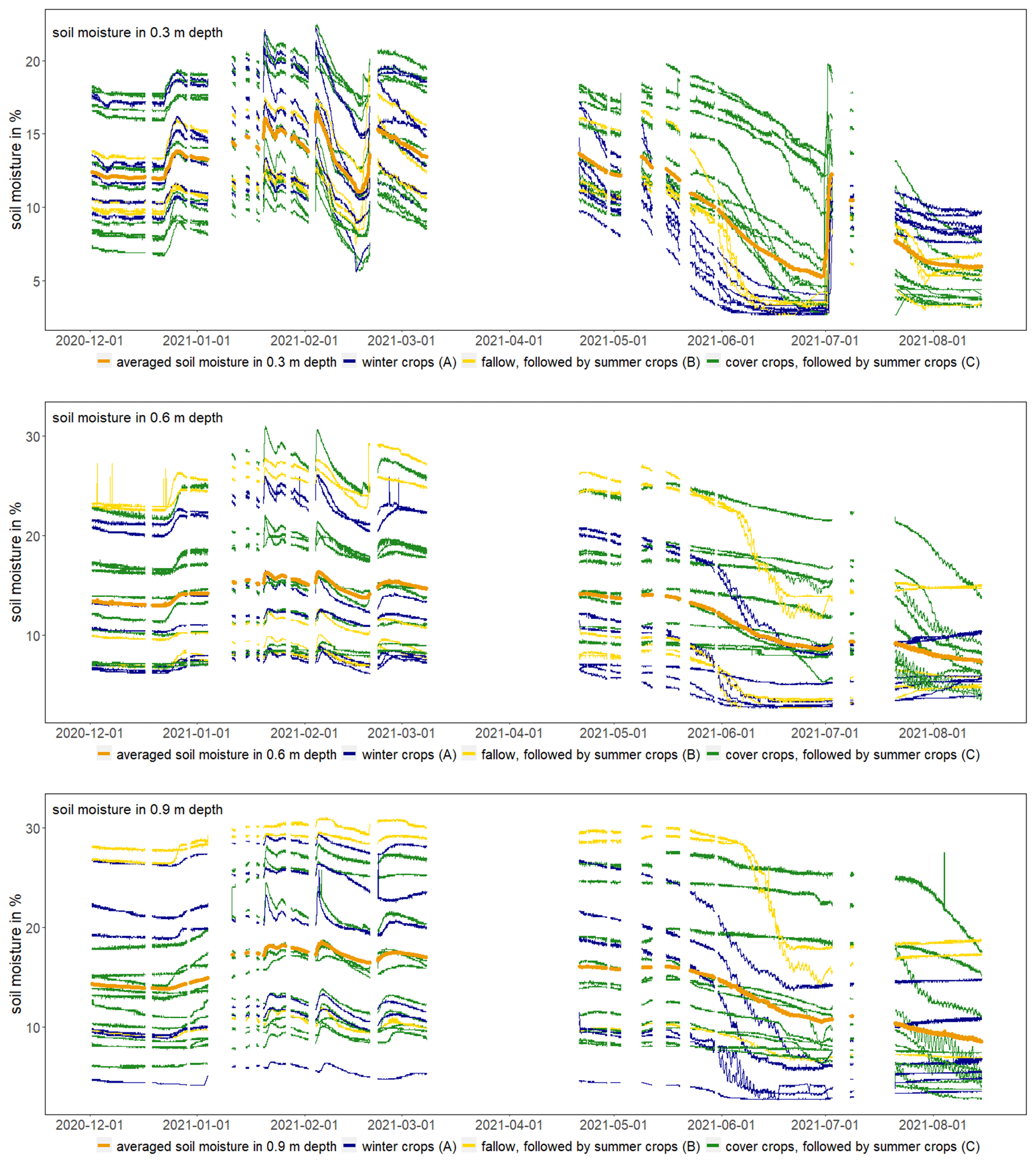
Figure 2 Input soil moisture time series per depth, differentiated between crop groups, and average soil moisture of all time series per depth from 1 December 2020 until 15 August 2021 at the patchCROP landscape experiment, Tempelberg, Brandenburg, Germany.

2.3 Data collection

2.3.1 Soil moisture data

Soil moisture was recorded by a long-range wide-area network (LoRaWAN)-based WSN. In each patch, one Dribox box equipped with an SDI-12 distributor (serial data interface at 1200 baud rate; model TBS04; TekBox, Ho Chi Minh City, Vietnam) connected to six TDR sensors (model TDR310H; Acclima, Meridian, MS, USA) and attached to an outdoor remote terminal unit (RTU) fully LoRaWAN-compliant (4 + 1 channel analogue to SDI-12 interface for 24 Bit A/D conversion of sensor signals; model TBS12B; TekBox, Ho Chi Minh City, Vietnam) was installed as a LoRa node. It was deployed at least 0.3 m below ground to allow field traffic and soil tillage. The sensors and boxes were installed between August and November 2020. At two georeferenced locations within each patch, soil moisture sensors were installed in 0.3, 0.6, and 0.9 m depth. Sensors were approximately 2 m from the LoRa node at angles between 45 and 60° (Fig. 1). Soil moisture sensors at 0.3 m were placed horizontally, while sensors at 0.6 and 0.9 m depth were placed vertically using auger-made boreholes and extension tubes for soil insertion. Communication of LoRa nodes was wireless and autarkic in energy supply. Thus, no electric cabling, except from connections between sensors and LoRa nodes, was needed. Under optimum conditions, the battery running time of the LoRa nodes can be up to 12 months but can be reduced to 8 months when radio transmission is attenuated (e.g. due to nearly water-saturated soil), which then increases power consumption (Bogena et al., 2009). Data were recorded every 20 min by the LoRa nodes through a LoRa-WAN Gateway DLOS8 (UP GmbH, Ibbenbüren, Germany), which was equipped with the modem TL-WA7510N (TP Link, Hong Kong SAR, China) to transfer the data to a cloud from which collected data could be accessed directly after the measurement. The time series included in this study covered the period from 1 December 2020 until 14 August 2021 (Fig. 2).

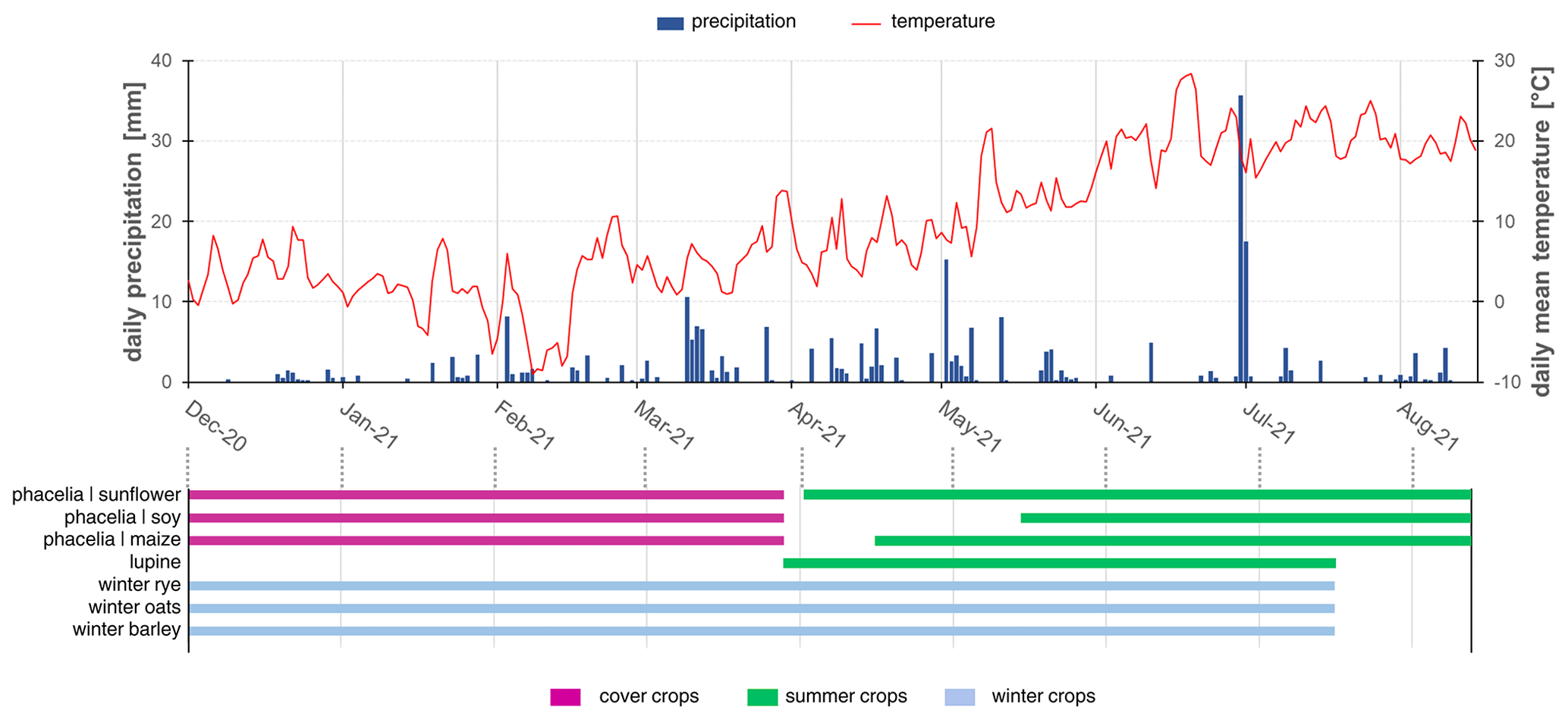
Figure 3 Measured daily precipitation, mean temperature, and cultivated crops – differentiated between winter crops (blue bars), summer crops (green bars), and cover crops (magenta bars) – from 1 December 2020 until 15 August 2021 at the patchCROP landscape experiment, Tempelberg, Brandenburg, Germany. Specific crops for the studied time frame are stated on the left side of the horizontal bars.

2.3.2 Weather data

Precipitation and temperature data (Fig. 3) with a 15 min temporal resolution were obtained from two weather stations located in the eastern and western ends of the main patchCROP field. Climatic water balance was calculated from precipitation and potential evapotranspiration, both measured at the climate station by the German Weather Service in Müncheberg (DWD Climate Data Center (CDC), 2021). This station was chosen due to its proximity to the study site.

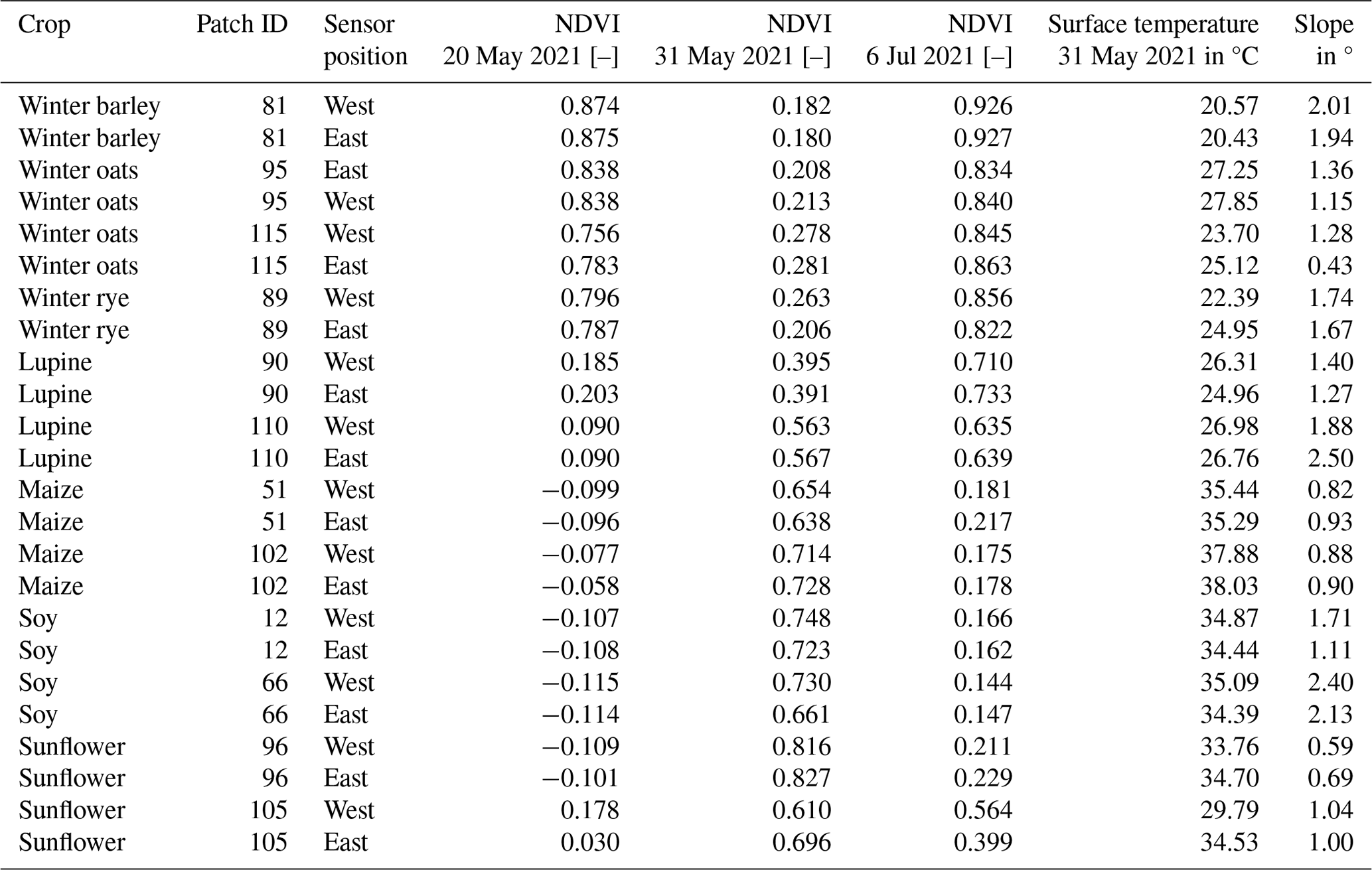
Table 2 Overview of normalized difference vegetation index (NDVI), surface temperature, and slope at the locations of analysed sensors in the patchCROP experiment in Tempelberg, Brandenburg, Germany.

2.3.3 Remote sensing data for vegetation dynamics

Drone imagery from 20 May 2021, 31 May 2021, and 6 July 2021 was used for vegetation assessment. The drone fixed-wing UAV-based RS eBee platform (SenseFly, Cheseaux–Lausanne, Switzerland) was operated at noon and recorded multispectral imagery with a Parrot Sequoia+ camera (green, red, near-infrared, and red edge bands; spatial resolution of 0.105 m) and thermal imagery of the surface (only on 31 May 2021) with a SenseFly Duet T camera with a spatial resolution of 0.091 m (Table 2). The multispectral imagery was processed with Pix4D to obtain the normalized difference vegetation index (NDVI) following Eq. (1):

$$\begin{array}{}\text{(1)}& \mathrm{NDVI}={\displaystyle \frac{\text{NIR}-\text{Red}}{\text{NIR}+\text{Red}}},\end{array}$$

in which NIR is the intensity of reflected near-infrared light (reflected by vegetation) and Red the intensity of reflected red light (absorbed by vegetation). A digital elevation model with a spatial resolution of 1 m (GeoBasis-DE and LGB, 2021) was used to calculate the slope (ArcGIS 10.7.0; ESRI, 2011) (Table 2).

2.3.4 Soil information

Soil texture by layer

Manual classification of soil texture by layer was carried out by collecting 140 samples in 8 of 12 analysed patches. Samples were taken with a 1 m long Pürckhauer soil auger. Soil textural class was manually determined at the field scale by applying the protocol “Finger test to determine soil texture according to DIN 19682-2 and KA5” (Sponagel et al., 2005). Additionally, representative soil samples were collected and analysed at the laboratory to determine particle size distribution for sand, silt, and clay (soil texture based on the German particle classification). Soil texture was analysed following the DIN ISO 11277 (2002) reference method by wet sieving and sedimentation using the Sedimat 4-12 (Umwelt-Geräte-Technik, Müncheberg, Germany). The sand fraction in this method is defined between 2 and 0.063 mm, according to IUSS Working Group WRB (2015).

To extrapolate the laboratory-based soil particle distribution to the soil textural classes manually determined at the field scale, the high- and low-yield-potential laboratory samples were pooled separately. The average soil particle distribution was calculated for each soil textural class and assigned to the respective soil layer with that specific soil textural class. The soil texture analysis showed that soil texture variability increased with depth. In the third layer (average bottom depth = 0.92 m), the sand and clay content across 133 sampling points varied between 53 % and 94 % and between 2 % and 22 %, respectively. Soil sampling points were located 0.8 and 2.5 m away from the soil moisture sensors to minimize damage risk.

Topsoil proximally sensed data

In October 2019, the Geophilus soil scanner system (Lueck and Ruehlmann, 2013) was used in the entire field to map soil electrical resistivity (ERa) as a proxy for texture for the topsoil using reference soil samples to calibrate the readings. A total of four georeferenced reference soil samples were taken until 0.25 m soil depth, and locations were selected based on the proximal soil sensor data (sensor-guided sampling; Bönecke et al., 2021). The Geophilus system is based on a sensor fusion in which ERa sensors are coupled with a gamma-ray detector. Apparent electrical conductivity was measured by pulling one or more sensor pairs mounted on wheels across the field where each pair of sensors measured a different soil depth. Amplitude and phase were measured simultaneously using frequencies from 1 MHz to 1 kHz. Reference soil samples were analysed via soil particle size analysis according to DIN ISO 11277 (2002) and served as calibration information in order to estimate sand, silt, and clay content in the top 0.25 m soil for the entire field. A non-linear regression model was applied. The RMSE of sand content (5.7 %) was considerably smaller than the standard deviation of the sand content in the first layer from the manual soil texture analysis (11.9 %), indicating a satisfactory prediction performance. The gamma sensor was used to minimize uncertainties, being less sensitive to soil moisture than the ERa readings (Bönecke et al., 2021). The estimated sand content in the upper 0.25 m at the study site varied between 69.1 % and 81.2 % and averaged 79.0 % (Fig. 1; Table 1).

2.4 Data processing

Soil moisture data were available at 20 min intervals. Transmission failures due to discharged batteries, signal disturbances after rainfall, high density of biomass in some patches (e.g. maize), and theft of parts of the WSN led to data gaps that affected in some cases all sensors of the WSN and amounted to 81 out of 257 d of the measuring period. The affected days were therefore skipped for the analysis. Whereas time series of eight sensors were excluded due to a higher frequency of transmission failures, in total, 64 time series were used for the analysis, and additional data gaps for single sensors were interpolated linearly. Of all 20 668 interpolated gaps, 96 % were shorter than 2 h, 3 % between 2 and 6 h, and 1 % longer than 6 h. In 26 cases, gaps exceeded the duration of 1 d. The interpolation was justified, as the differences between the values before and after the gaps were within the measuring accuracy of ±3 vol % of the soil moisture sensors (Acclima Inc., 2023). As indicated by the retailer, sensors might suddenly jump to a soil moisture value of 28.6 % and go back to normal again after one or a few time steps. Thus, a data deletion procedure of abrupt jumps to 28.6 was created. To ensure equal weighting for the subsequent analysis, all soil moisture time series were z-transformed to unit variance and zero mean each (see Hohenbrink and Lischeid, 2015). As a consequence, differences in absolute values were not considered by the further analysis.

2.5 Statistical analysis

To identify common temporal patterns among single time series, the soil moisture data set was analysed by a principal component analysis (PCA). In a first step, PCA decomposes the total variance of a multivariate data set into independent fractions called principal components (PCs). The number of PCs is the same as the number of time series in the input data set. Each PC consists of eigenvectors (loadings), scores, and eigenvalues. The scores reflect the temporal dynamics. The importance of single principal components for single sites is represented by the loadings of each PC (Jolliffe, 2002; Lehr and Lischeid, 2020). Loadings are the Pearson correlation coefficients of the single time series of the input data set with the scores of each PC, respectively. The eigenvalues of the single PC are proportional to the variance that they explain. The PCs are sorted in descending order of eigenvalues. Eigenvalues greater than 1 indicate that a PC explains more variance than a single input time series could contribute to the total variance of the entire input data set (Kaiser, 1960). More details on principal component analysis for time series analysis are found in Jolliffe (2002). The PCA was performed using the prcomp function in R version 4.1.0 (R Development Core Team, 2021).

The scores of the principal components constitute time series. Every observed soil moisture z-transformed time series can be presented at arbitrary precision as a combination of various principal components. When the data set consists of time series of the same observable measured at different locations, the first principal component describes the mean behaviour inherent in the data set. Subsequent principal components reflect typical modifications of that mean behaviour at single locations due to different effects. Thus, generating synthetic time series as linear combinations of the first PC and another additional PC helps to assign this additional PC to a specific effect. To that end, scores of that component have either been added to or subtracted from those of the first component using arbitrarily selected factors. The two resulting graphs show how the respective PC causes deviations from the mean behaviour of the data set.

The relations to soil and vegetation parameters were tested by computing the Pearson correlation coefficients between the scores and arithmetic mean values of all input time series as well as the Pearson correlation coefficients between loadings and sand content until 0.25 m depth, sensor depth, antecedent z-transformed soil moisture, slope, and drone imagery products (NDVI and surface temperature). Eventually, the Wilcoxon–Mann–Whitney test was applied to check whether loadings could be grouped by management parameters (i.e. crops, cover crops, and weeding management). All statistical analyses were conducted with R version 4.1.0 (R Development Core Team, 2021).

3 Results

3.1 Manual soil texture analysis

The transferability of texture information from the sampling point to the soil moisture sensor location was not ensured due to high nugget effects. Furthermore, manual soil texture analysis data were not available for all analysed patches. Consequently, they were not included in further analysis.

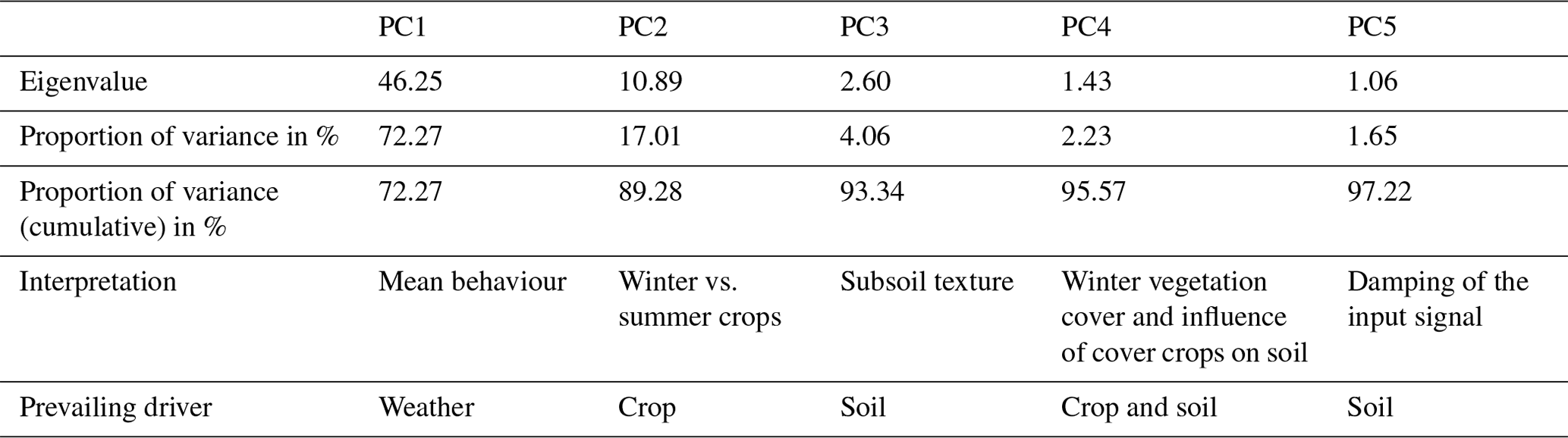
Table 3 Statistical characteristics and interpretations of principal components 1–5 for soil moisture dynamics of selected patches at the patchCROP landscape experiment in Tempelberg, Brandenburg, Germany.

3.2 Principal component analysis

The principal component analysis yielded five components with eigenvalues exceeding 1, which accounted for > 97 % of the total variance of the data set (Table 3).

3.2.1 First principal component

The first principal component explained 72.3 % of the spatiotemporal variance in the data set. All loadings on the first PC were negative (see Appendix A). The Pearson correlation coefficient of the scores of the first principal component with the mean values of all input time series was less than −0.999 (p < 0.01), and the correlation between the scores and the cumulative climatic water balance (P−ET_p) was −0.969 (p < 0.01). Thus, the time series of the negative scores of this component represented the mean behaviour of soil moisture driven by external factors such as precipitation, temperature, and seasons in general which affected all time series in the same way, although to different degrees (see Hohenbrink et al., 2016; Lischeid et al., 2021).

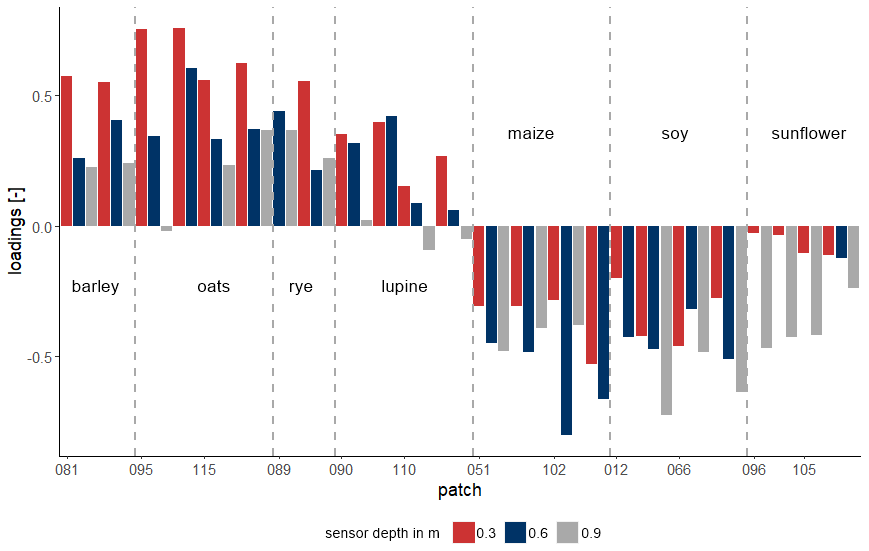
Figure 4 Time series loadings on the second principal component at the patchCROP landscape experiment in Tempelberg, Brandenburg, Germany, showing a crop-group-related pattern. Bars represent individual time series grouped by patch ID and sorted by crop.

3.2.2 Second principal component

The second principal component explained 17.0 % of the total variance. The loadings ranged from −0.801 to 0.760 with a median of −0.030 (Fig. 4). The loadings showed a crop-group-specific pattern. All winter crops (barley, oats, and rye) had positive loadings with only one exception in 0.9 m depth. The summer crops maize, soy, and sunflower exhibited negative loadings. In contrast, the summer crop lupine exhibited mostly positive loadings, similar to the winter crops, although of slightly smaller magnitude. According to the Wilcoxon–Mann test, the group of barley, oats, rye, and lupine differed significantly from the group of maize, soy, and sunflower.

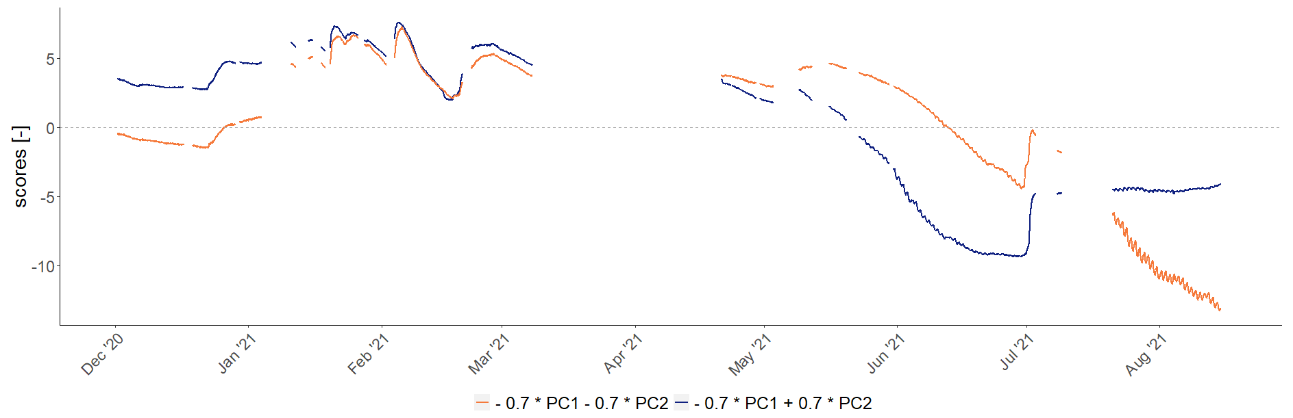
Figure 5 Effect of the second principal component on modification of the general mean behaviour presented by the first principal component at the patchCROP landscape experiment in Tempelberg, Brandenburg, Germany. The blue line represents deviations from mean soil moisture for time series with positive loadings on PC2 (winter crops), while the orange line represents deviations from mean soil moisture for time series with negative loadings on PC2 (summer crops).

As described in the “Materials and methods” section, synthetic time series were generated as a linear combination of PC1 and PC2 as shown in Fig. 5. The graph resulting from applying a positive factor for PC2 represents a typical deviation from mean behaviour for sites that exhibit positive loadings, e.g. winter crops (blue line). The opposite holds for the summer crops which load negatively on PC2 (orange line). Both lines plot very close to each other in February and March. In contrast, the orange line shows lower values than the blue line in December and January, indicating lower soil moisture at the summer crop patches. The inverse holds for the subsequent summer period starting in early June, pointing to earlier and more rapid water uptake of the winter crops. In July and August, the approximately constant level of the blue curve indicates that only summer crops continue to consume water, while winter crops are in their ripening phase and eventually harvested.

Lupine and sunflower were the summer crops which were sown first (30 March 2021 and 21 April 2021, respectively). Maize was sown on 16 April 2021 and soy on 15 May 2021. The loadings of lupine, which performed like winter crops rather than summer crops, indicated that lupine showed an early onset of intensive evapotranspiration compared with other summer crops, especially sunflower, which was sown at the same time.

Table 4 Pearson correlation coefficients between surface temperature and normalized difference vegetation index (NDVI) at the patchCROP landscape experiment (Tempelberg, Brandenburg, Germany) and loadings of sensors in all depths or at single depths, respectively, on the second principal component. All correlations were highly significant (p < 0.01).

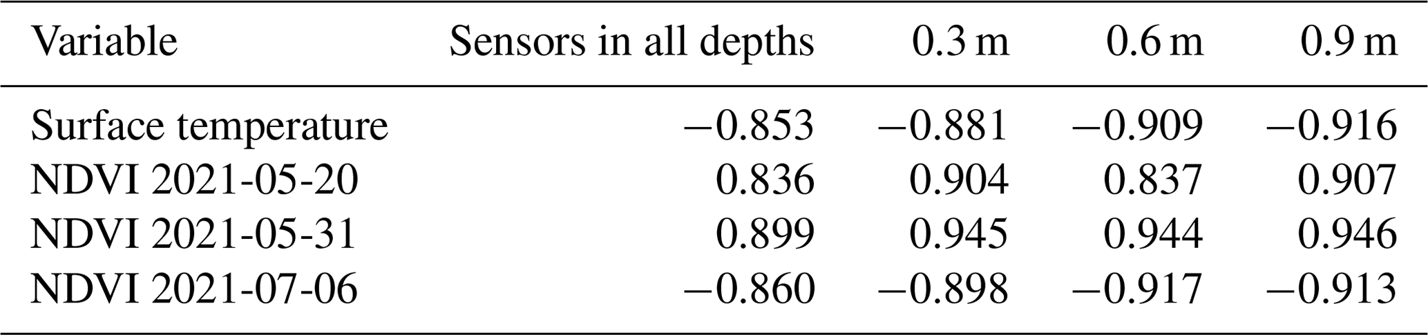
For further investigation of the vegetation effect on PCs, drone imagery taken at the end of May, when sowing has been completed in all patches, and imagery taken at the beginning of July, when winter crops are in the ripening phase, were analysed. The second PC's loadings of the time series from different sensors were compared with the normalized difference vegetation index (NDVI; available for three dates) and surface temperature (only available for 31 May 2021) of the respective sensor location as a proxy for actual evapotranspiration. At the end of May, the NDVI, as a proxy for photosynthesis potential, was positively correlated with the loadings (Table 4). Surface temperature exhibited a negative correlation. The spatial pattern of surface temperature is assumed to be inversely related to that of actual evapotranspiration. Thus, both proxies, NDVI and surface temperature, support the inference that in this study positive loadings on this principal component represent sites with above-average plant activity and root water uptake at the end of May. This holds for sensors from all depths but was the closest for 0.9 m depth (Pearson correlation of r = −0.916 for surface temperature and r = 0.946 for NDVI on 31 May). The results in July compared with those in May support the observation. At the time when the winter crops are already in the ripening phase and the summer crops reach high levels of evapotranspiration, the correlations are reversed and negative loadings indicate above-average plant activity for summer crops. On 6 July, the highest Pearson correlations for NDVI are found for 0.6 m depth (r = −0.917).

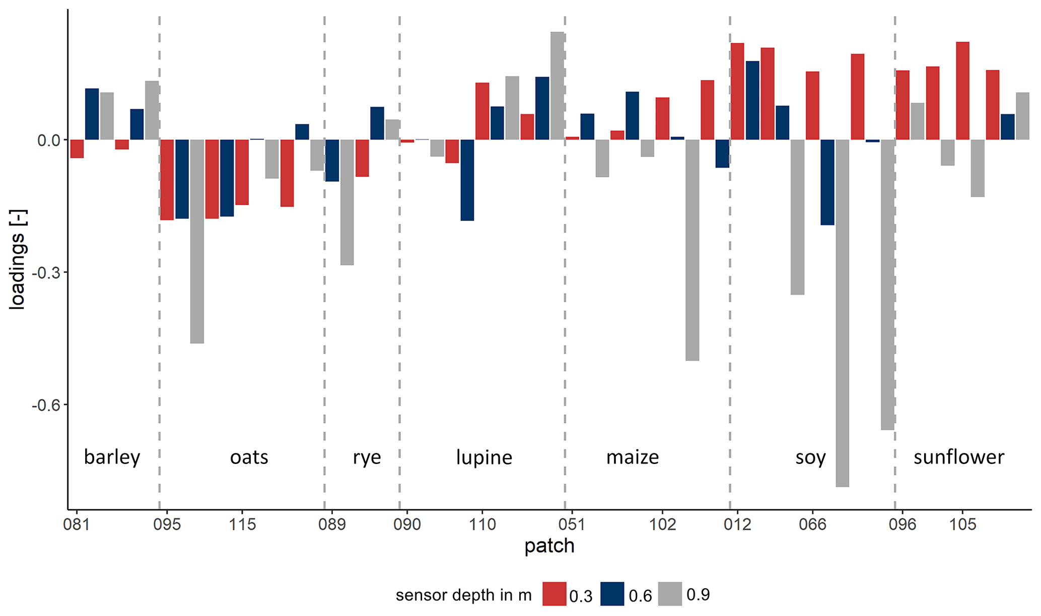
Figure 6 Loadings of time series on the third principal component at the patchCROP landscape experiment (Tempelberg, Brandenburg, Germany) with some of the sensors in deeper layers showing noticeably negative loadings. Bars represent individual time series grouped by patch ID and sorted by crop.

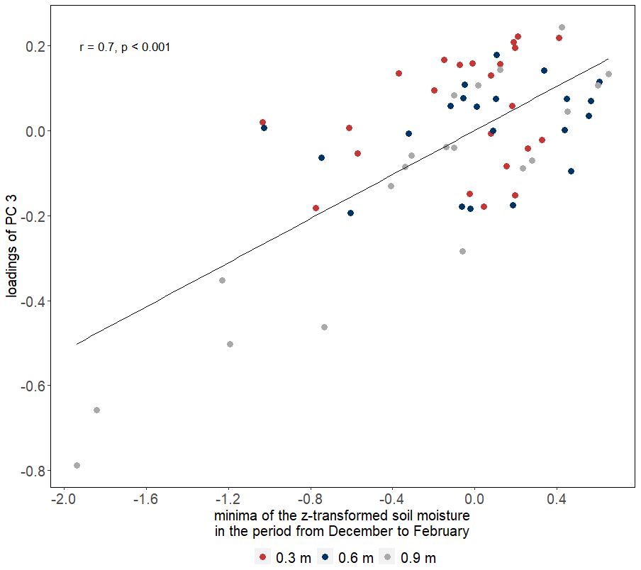
Figure 7 Relation between minima of the z-transformed soil moisture in the first months of the study period and loadings of the third principal component showing that sensors with noticeably negative loadings showed distinctly negative z-transformed minima.

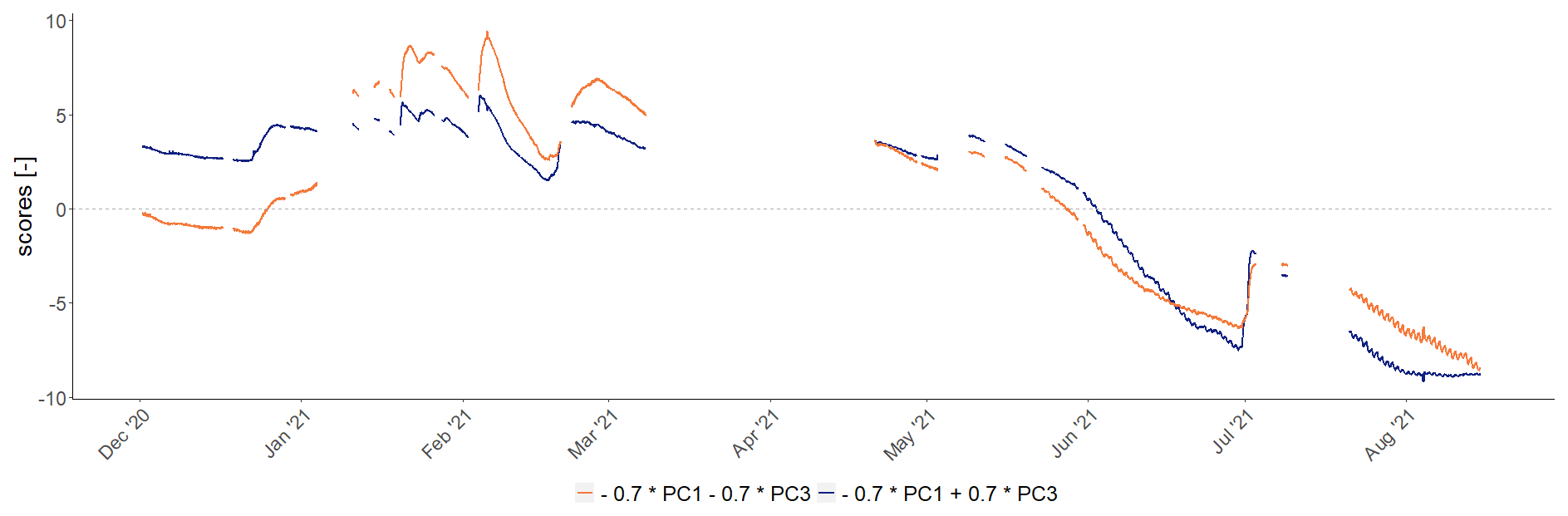
Figure 8 Effect of the third principal component on modification of the general mean behaviour presented by the first principal component at the patchCROP landscape experiment in Tempelberg, Brandenburg, Germany. The blue line represents deviations from mean soil moisture for time series with positive loadings on PC3 (majority of the time series), while the orange line represents deviations from mean soil moisture for time series with negative loadings on PC3 (some of the sensors in 0.9 m depth).

3.2.3 Third principal component

The third PC explained 4.1 % of the total data set's variance. Loadings ranged between −0.787 and 0.244 with a median of 0.006. Extreme loadings (< −0.25) were found only for sensors in 0.9 m depth in patches 66, 89, 95, and 102 (Fig. 6). The locations of these patches show a certain spatial pattern, with the patches roughly following an east–west direction rather than being distributed randomly within the field. This may point to topography or soil structure causing deviations from mean soil moisture behaviour for patches located near this gradient. However, this pattern cannot be assigned to topography or structures apparent on the topsoil map (Fig. 1). Loadings were closely related to the minima of the z-transformed soil moisture in the period from December to February (r = 0.70, p < 0.001; Fig. 7). What distinguishes the orange line (negative loading on PC3) from the blue line (positive loading on PC3) in Fig. 8 is the higher temporal variability and the delayed reaching of maxima in the first half of the study period.

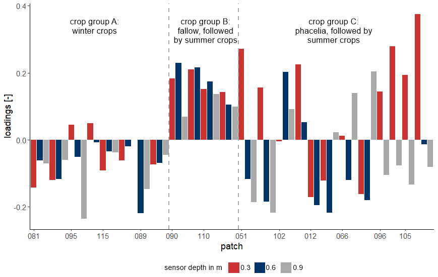
Figure 9 Loadings of time series on the fourth principal component at the patchCROP landscape experiment (Tempelberg, Brandenburg, Germany) showing mainly negative loadings for crop group A, positive loadings for crop group B, and loadings with no clear pattern for crop group C. Bars represent individual time series grouped by patch ID and sorted by treatment group.

3.2.4 Fourth principal component

The fourth PC explained 2.2 % of the total data set's variance. The loadings were clustered by crop groups. All fallow patches showed consistent positive loadings, while the patches which were covered by winter crops showed mainly negative loadings except in patch 95 where the loadings of the two sensors in 0.3 m depth were slightly above zero (Fig. 9). According to the Wilcoxon–Mann test, treatment group B (fallow followed by summer crops) differed significantly from group A (winter crops) and C (cover crops followed by summer crops), whereas there was no significant difference between groups A and C. In contrast to crop groups A and B, patches that were covered by the cover crop Phacelia during the winter months did not show one-directional loadings.

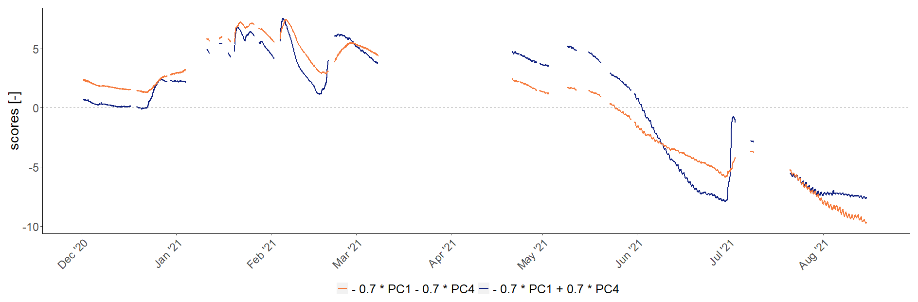
Figure 10 Effect of the fourth principal component on modification of the general mean behaviour presented by the first principal component at the patchCROP landscape experiment. The blue line represents deviations from mean soil moisture for time series with positive loadings on PC4 (single sensors of crop group A, all sensors of crop group B, and part of crop group C), while the orange line represents deviations from mean soil moisture for time series with negative loadings on PC4 (most sensors of crop group A and part of the sensors of crop group C).

Figure 10 illustrates the effect of the fourth PC on time series. The blue line (positive loading) shows hydrological behaviour which would be typical for more sandy soils, while the orange line (negative loading) depicts behaviour that one would expect in more loamy soils due to its delayed responses to rainstorms and subsequent less steep recovery. The patterns in the loadings thus show a differentiation between patches with winter crops and fallow patches in the winter months (Fig. 9). However, it is not clear how winter crops on the one side and fallow patches on the other side could induce such different soil water behaviour as shown in Fig. 10.

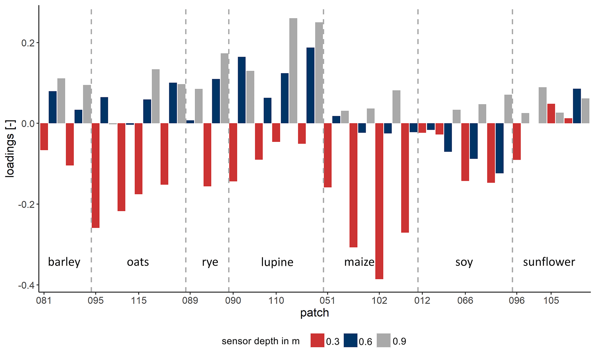
Figure 11 Loadings of time series on the fifth principal component at the patchCROP landscape experiment showing a depth-related pattern. Bars represent individual time series grouped by patch ID and sorted by crop.

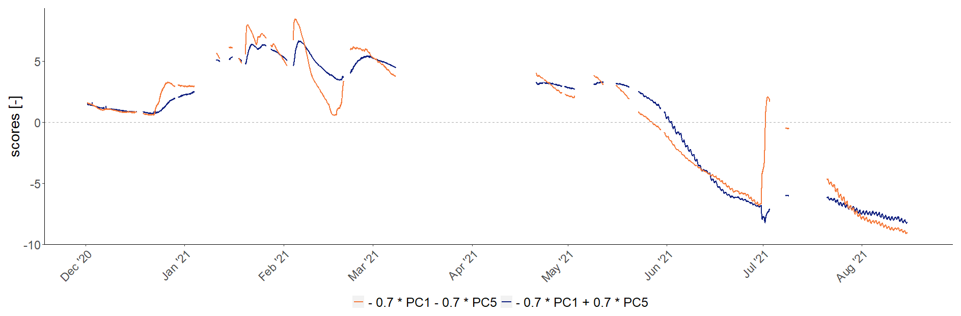
Figure 12 Effect of the fifth principal component on modification of the general mean behaviour presented by the first principal component at the patchCROP landscape experiment, Tempelberg. The blue line represents deviations from mean soil moisture for time series with positive loadings on PC5 (sensors in greater depth), while the orange line represents deviations from mean soil moisture for time series with negative loadings on PC5 (sensors in shallow depth).

3.2.5 Fifth principal component

The fifth PC explained 1.7 % of the data set's variance. The loadings showed a depth-related pattern. All time series from 0.3 m depth exhibited negative loadings with two minor exceptions in patch 105. Except for patch 95, all time series from 0.9 m depth showed positive loadings. Loadings in 0.6 m depth and 0.9 m depth were mostly more similar to each other than to the loadings in 0.3 m depth (Fig. 11). The Pearson correlation coefficient between loadings and depth was r = 0.710 (p < 0.05). Thus, it can be concluded that the fifth PC reflected the effect of soil depth on soil moisture variance. This effect differed between crops, with the three most negative loadings found in maize patches and the three most positive loadings found in lupine patches. In Fig. 12 the soil water dynamics show a damping effect with increasing depth from little damping for sensors in the upper depth (orange line) to higher damping for sensors in greater depth (blue line).

Patterns in neither topography nor weeding management modes were reflected in the loadings of PC1–PC5. Due to the lack of subsurface soil data, no additional findings could be derived from the Geophilus texture analysis.

4 Discussion

A PCA was conducted to identify the drivers of soil moisture variability in a diversified cropping field. Data consisted of observed time series from 64 soil moisture probes. Results showed that the first five principal components described about 97 % of the variance of the data set and revealed various effects of weather, soil texture, soil depth, crops, and management schemes (Table 3). The first principal component captured 72 % of the total variance. Consequently, 72 % of the observed dynamics could be described by a lumped model that would not consider any within-field heterogeneity. These results are in the range of similar studies. Martini et al. (2017) found that the first PC explained 58 % of the variance in a data set that comprised both agricultural fields and grassland transects. Similarly, Lischeid et al. (2017) ascribed 70 % of the variance in a forest soil moisture data set to a single component. In the study by Hohenbrink et al. (2016), 85 % of the variance in soil moisture data in a set of arable field experiments with two different crop rotation schemes was attributed to the first principal component. The strong influence of weather conditions as shown in our study is confirmed by Choi et al. (2007), who showed that rainfall, next to topography, explained most of the surface soil moisture variability.

4.1 Crop effects

As Korres et al. (2015) stated, vegetation and management (e.g. planting and harvesting dates) are among the main causes for spatial variability in soil moisture in agricultural fields. In this study, around 17 % of the total variance at the field scale was attributed to the vegetation effect. When not considering the temporal component reflected by PC1 and thus only looking at the spatial variability, 61 % of the remaining variance is caused by the vegetation effect reflected by PC2. Korres et al. (2010) also used PCA to identify the drivers of spatial variability in soil moisture within a cropped area but did not find such a pronounced vegetation effect. In their study, more than two-thirds of the spatial variability was related to soil parameters and topography. In contrast, the strong influence of vegetation in our study may be due to the high level of crop diversification. Within single crop fields, vegetation effects are observable due to heterogeneous biomass or root development (Brown et al., 2021; Korres et al., 2010) but may be of a lower magnitude compared with fragmented field arrangements with different crops. The high impact of crop diversification on soil moisture variability is also visible when comparing our results with the results of a field under comparable conditions in the same region with only two crop rotations in which only 3.8 % was explained by the different crop rotations (Hohenbrink et al., 2016). Joshi and Mohanty (2010) also assessed the effect of vegetation in their study in which they investigated spatial soil moisture variability at the field to regional scale in the southern Great Plains regions in the USA by means of PCA. With none of the first seven PCs showing strong correlation with vegetation parameters, the effect of vegetation was limited in contrast to our study.

It needs to be considered that the proportion of the vegetation effect on soil moisture variability varies not only spatially and over depth, but also over time. Under dry conditions, soil–plant interactions prevail, while under moist conditions, percolation behaviour is predominant (Baroni et al., 2013). The scores are time series and reflect the effect size of a particular process represented by the respective PC. The more the scores of a certain PC deviate from zero during specific periods, the stronger the respective effect is. Consequently, the time series of PC2 scores indicates that the effect of vegetation on total variability varies with time. In accordance with the literature, the absolute values of the scores of PC2, representing differences between the contrasting seasonality of crops, are highest in the dry months, May to August. This is mostly explained by the high water demand of summer crops, which are in their vegetative growth stage from May to August, whereas winter crops are already in their reproductive growth stage, including maturity, senescence, and harvest where water uptake by crops is minimal or absent (Zhao et al., 2018). In the moist winter months of January to March, as well as during the heavy rainfall event in July, the scores of PC2 are relatively small, showing that spatial variability at that time is caused by other factors.

The second principal component clearly differentiated between winter and summer crops and was driven by the different seasonal patterns of root water uptake (Fig. 4). In contrast, the fourth component differentiated between fallow patches followed by summer crops and winter crops, whereas Phacelia followed by summer crops did not show a clear pattern (Fig. 9). Phacelia is grown as a cover crop and usually dies off in frost periods. Due to rather mild winter temperatures during 2020–2021, Phacelia was not terminated efficiently and kept growing until spring, until it was terminated mechanically. It was recently shown that the timing of removal of winter cover crops is key to providing soil water recharge for the subsequent crops, as the depletion of soil water in autumn is significant (Selzer and Schubert, 2023). Thus, some Phacelia patches exhibited negative loadings, similarly to the winter crop patches, while other patches with most likely different termination dates exhibited positive loadings.

Hence, the fourth component obviously reflected the effect of the active root system in the winter period. According to this component, soil water dynamics in the fallow patches mostly resembled the typical behaviour expected for sandy soils and winter crop patches showed a more damped behaviour that is usually observed in more loamy soils. (Note that the term “fallow” refers to crop cover in autumn and winter only.) Acharya et al. (2019) found that winter cover crops increased soil moisture from 3 % to 5 % in the top 0.3 m soil layer; this is in line with the findings in Fig. 10, which shows a higher water-holding capacity for winter crops (orange line) in winter. However, it has also been observed that roots from winter crops can increase soil porosity and therefore water mobility in the soil (Lange et al., 2013; Scholl et al., 2014).

Further soil–vegetation interactions might play a role for the delayed seepage fluxes of winter crop and part of cover crop patches, such as soil organic content increase through the presence of cover crops and plant residues (Manns et al., 2014; Rossini et al., 2021). Usually, such effects are assumed to occur only at larger timescales, which is closely related to problems of detecting changes in soil organic carbon (SOC) quantity or quality. So far, there is only anecdotal evidence for rather short-term SOC quality changes affecting soil hydraulic properties even at smaller timescales. Although this effect constituted only a minor share of soil moisture variance (Table 3), it was clearly discernible as a separate principal component. This effect would be worth testing in more detailed future studies.

4.2 Soil texture and soil depth effects

Loadings on the third principal component were not related to crop types. In contrast, a spatial pattern emerged: only sensors from 0.9 m depth from six adjacent patches exhibited strongly negative loadings (Fig. 6), whereas all other sensors showed minor positive or negative loadings. This points to an effect of subsoil substrates: that is, higher clay content and consequently higher water-holding capacity. That would be consistent with delayed response to seepage fluxes and reduced desiccation in the vegetation period (Fig. 8). The strong relation between z-transformed soil moisture minima at the beginning of the study period (Fig. 7), which might originate from a delayed response to a prior rainfall, and the regional pattern of the location of the patches following a west–east direction within the experiment might be an indicator of underlying soil structures causing this effect. Data on texture at soil moisture sensor locations in deeper layers would be of high value to confirm the assumptions.

Whereas the third principal component seems to reflect a local peculiarity, the fifth component obviously grasps a more generic feature. Loadings on this component are clearly related to depth (Fig. 11). Strong positive loadings indicate a strongly damped behaviour of soil moisture time series: in Fig. 12, the blue line, representing sites with positive loadings on PC5 which is typical for sensors at greater depth, exhibits clearly reduced amplitudes compared with the orange line, which represents sensors at shallow depth. Hohenbrink and Lischeid (2015) combined a hydrological model and principal component analysis to study the effect of soil depth and soil texture on damping of the input signal in more detail. A subsequent field study proved the relevance of that effect in a real-world setting (Hohenbrink et al., 2016). Moreover, Thomas et al. (2012) found that damping accounted for a large share of variance in a set of hydrographs from a region of 30 000 km². Damping was also the most relevant driver of spatial variance in a set of time series of groundwater head at about the same scale (Lischeid et al., 2021).

4.3 Limitations

Data gaps during the studied period occurred due to multiple technical and environmental factors. Data gaps in soil moisture time series were caused by repeated temporary failure of the WSN. There was a failure of one sensor that was replaced and one LoRa node was damaged by intruding water. More relevant, however, were failures of data transmission. Yildiz et al. (2015) point to the problem of optimizing transmission power for data and acknowledgement packets depending on energy dissipation under the given conditions. For example, saturated soil conditions and dense biomass stands reduce the transmission signal from the node to the gateway (Bogena et al., 2009). The installation of a second gateway in September 2021 increased higher transmission coverage in the field. Another obstacle was snow cover on the gateways' solar panels. Finally, solar panels were subject to theft. However, a higher level of maintenance and supervision helped to reduce the number and the length of data gaps.

PCA requires gapless time series. Gaps in single time series either need to be filled at the risk of introducing artefacts or the respective time period cannot be considered at all for analysis. This can be seen as a weakness of PCA. On the other hand, and in contrast to other time series analysis approaches, the time series need not be equidistant. Assigning PCs to processes and effects is not straightforward and might be a subject for debate. For example, in this study soil samples were taken at least 0.8 m from the sensors to avoid disturbance in the measurements. Due to pronounced small-scale soil variability, these samples are not fully representative of the measurement sites. In spite of these limitations, the PCA results clearly point to various effects worth further study in more detail in subsequent work.

5 Conclusion

The use of PCA is quite valuable for application in environmental sciences, as it contributes to process understanding of soil water dynamics by disentangling the different effects of complex spatially and temporally diversified cropping systems. In this study, more than 97 % of the observed spatial and temporal variance was assigned to five different effects. Meteorological drivers explained 72.3 % of the total variance (PC1). Different seasonal patterns of root water uptake of winter crops compared with summer crops accounted for another 17.0 % of variance (PC2). An additional share of 2.2 % of variance seemed to be related to the effects of different vegetation cover and its interplay with soil hydraulic properties (PC4). Heterogeneity of subsoil substrates explained 4.1 % of variance (PC3) and the damping effect of input signals over depth another 1.7 % (PC5). To summarize, plant-related direct and indirect effects accounted for 19.2 % of the variance (PC2 and PC4), and soil-related effects for only 5.8 % (PC3 and PC5). In particular, the plant-induced effects on soil hydraulic properties would be worth studying in more detail.

Findings of this study highly depend on local conditions. However, the methodology itself is generally applicable to other site conditions and can lead to improved management practices through improved knowledge about soil water dynamics. Furthermore, information from this study can also help in developing both parsimonious and tailored mechanistic models for model upscaling. In this regard, principal component analysis of large soil moisture data sets from real-world monitoring setups can be performed as a meaningful diagnostic tool for complex cropping systems.

Appendix A

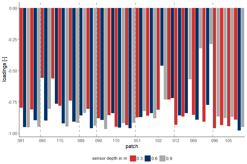
Figure A1 Loadings of time series on the first principal component at the patchCROP landscape experiment, Tempelberg, Brandenburg, Germany. Bars represent individual time series grouped by patch ID and sorted by crop.