the Creative Commons Attribution 4.0 License.
the Creative Commons Attribution 4.0 License.
 | 05 Jun 2024
Machine learning and global vegetation: random forests for downscaling and gap filling
Barry van Jaarsveld
Sandra M. Hauswirth
Niko Wanders
Drought is a devastating natural disaster, during which water shortage often manifests itself in the health of vegetation. Unfortunately, it is difficult to obtain high-resolution vegetation drought impact information that is spatially and temporally consistent. While remotely sensed products can provide part of this information, they often suffer from data gaps and limitations with respect to their spatial or temporal resolution. A persistent feature among remote-sensing products is the trade-off between the spatial resolution and revisit time: high temporal resolution is met with coarse spatial resolution and vice versa. Machine learning methods have been successfully applied in a wide range of remote-sensing and hydrological studies. However, global applications to resolve drought impacts on vegetation dynamics still need to be made available, as there is significant potential for such a product to aid with improved drought impact monitoring. To this end, this study predicted global vegetation dynamics based on the enhanced vegetation index (evi) and the popular Random forest (RF) regressor algorithm at 0.1°. We assessed the applicability of RF as a gap-filling and downscaling tool to generate global evi estimates that are spatially and temporally consistent. To do this, we trained an RF regressor with 0.1° evi data, using a host of features indicative of the water and energy balances experienced by vegetation, and evaluated the performance of this new product. Next, to test whether the RF is robust in terms of spatial resolution, we downscale the global evi: the model trained on 0.1° data is used to predict evi at a 0.01° resolution. The results show that the RF can capture global evi dynamics at both a 0.1° resolution (RMSE: 0.02–0.4) and at a finer 0.01° resolution (RMSE: 0.04–0.6). Overall errors were higher in the downscaled 0.01° product compared with the 0.1° product. Nevertheless, relative increases remained small, demonstrating that RF can be used to create downscaled and temporally consistent evi products. Additional error analysis revealed that errors vary spatiotemporally, with underrepresented land cover types and periods of extreme vegetation conditions having the highest errors. Finally, this model is used to produce global, spatially continuous evi products at both a 0.1 and 0.01° spatial resolution for 2003–2013 at an 8 d frequency.
- Article
(6686 KB) - Full-text XML
- BibTeX
- EndNote


The impacts of natural hazards are felt at a local scale, but creating impactful risk management strategies requires a global view regarding the driving processes and impacts (Ward et al., 2020). Given its complex and multivariate nature, a global perspective is especially necessary when considering drought hazards. Drought is one of the most disruptive natural hazards, causing negative repercussions for the environment, economy, and society and potentially affecting large areas and populations (Naumann et al., 2014; Vereinte Nationen, 2021). However, a universal definition of what constitutes a drought event remains elusive. As a result, we lack a comprehensive understanding of the direct and indirect effects of drought on the environment and society (Blauhut et al., 2016; Vogt et al., 2018; Sutanto et al., 2019). Remotely sensed products that monitor Earth system responses during drought periods are one promising tool that can enable a global perspective on drought hazards and their impacts (AghaKouchak et al., 2015; West et al., 2019). However, they suffer from trade-offs between spatial and temporal resolution: we either have high-resolution, low-frequency products or the inverse. The production of high-resolution, spatially continuous products can facilitate a more holistic view of drought responses and management by incorporating more relevant fine-scale processes (Chen et al., 2022; Schneider et al., 2017).
Vegetation is involved in numerous drought impact pathways, and using remote sensing to track vegetation responses has been widely used (Y. Zhang et al., 2021; AghaKouchak et al., 2015). Drought disrupts terrestrial water and carbon cycles, which can reduce the integrity of ecosystem dynamics and associated ecosystem services (Banerjee et al., 2013; Crausbay et al., 2017; Han et al., 2018; Smith et al., 2020). More subtly, vegetation also affects the dynamics of drought propagation itself; under favourable antecedent conditions, vegetation overshoot may exacerbate and facilitate the onset of rapid and intense droughts (Y. Zhang et al., 2021). Vegetation is also expected to play a crucial role in shaping drought resistance under future climate change (Vereinte Nationen, 2021). In the absence of such resistance, interventions to alleviate the negative impacts of disrupted ecosystem services can cost up to USD 1 billion per drought event (Banerjee et al., 2013; Cammalleri et al., 2020). It follows that formulating appropriate responses to drought and alleviating the negative effects of ecosystem disruption during these periods requires accurate predictions.
In recent decades, numerous satellite-based vegetation indices have been developed (S. Li et al., 2021). For example, the enhanced vegetation index (evi) has proven to be an indispensable tool for monitoring vegetation at multiple scales, from the fine scale, such as crop patches (Moussa Kourouma et al., 2021; Sharifi, 2021), to the global scale (Huang et al., 2021; Vicente-Serrano et al., 2010). However, a persistent feature among these products is the trade-off between the spatial resolution and revisit time: high temporal resolution is met with coarse spatial resolution and vice versa. For example, the Moderate Resolution Imaging Spectroradiometer (MODIS) captures the entire Earth at high temporal resolution every 1 to 2 d (Zhao and Duan, 2020) with a maximum spatial resolution of 250 m. Landsat and Sentinel-2 data have a higher spatial resolution (10 and 30 m, respectively) but longer revisit periods of approximately 10 and 5 d, respectively (Zhu, 2017; S. Li et al., 2021). Revisit times for Landsat and Sentinel-2 are further prolonged when sensors or retrievals are interrupted by cloud cover, pollution in the atmosphere, or even technical issues. In addition to the temporal frequency, temporal coverage is another important consideration. Coarser-scale products are associated with older satellites and have more extended temporal coverage than the newer ones; MODIS products reach as far back as 1999, whereas Sentinel-2 products only go back to 2017. The ideal product for monitoring vegetation dynamics would have global coverage, few to no data gaps, and high spatial and temporal resolution.
Machine learning (ML) methods have been used for downscaling and gap-filling purposes in remote-sensing products; thus, they can be seen as one tool that can lead to the production of high-quality remote-sensing products, thereby alleviating the resolution and coverage limitations that current products exhibit (Zhu et al., 2022; Zeng et al., 2013). ML methods have been successfully applied to a wide range of drought-related (Hauswirth et al., 2021; Shamshirband et al., 2020; Tufaner and Özbeyaz, 2020; Shen et al., 2019; Das et al., 2020; Hauswirth et al., 2023) and remotely detected vegetation studies (Roy, 2021; X. Li et al., 2021; Reichstein et al., 2019). Compared with conventional statistical downscaling techniques, ML is considered the superior alternative, as no strict statistical assumptions are required, complex and nonlinear relationships are well captured, and it provides high precision (Ebrahimy et al., 2021).
One ML algorithm that has been widely applied for gap filling and downscaling of remote-sensing data is the Random forest (RF) regressor (J. Zhang et al., 2021; Fu et al., 2022; Liu et al., 2020; Wang et al., 2022). Gap filling can be achieved by training an RF on available data and then using the model to predict values where data are sparse or missing (Wang et al., 2022). Using RF to downscale data involves the establishment of an RF at a coarse scale and the prediction of targets at finer resolutions by feeding the algorithm with high-resolution auxiliary data (Liu et al., 2020). These studies have highlighted that ML methods can accurately predict the dynamics of vegetation (Roy, 2021; Gensheimer et al., 2022). However, studies applying ML methods to global vegetation dynamics and assessing their suitability to investigate drought responses are less prominent, and it remains to be seen whether this approach is applicable at the global scale (X. Li et al., 2021; Y. Zhang et al., 2021; Chen et al., 2021).
This study aims to further our understanding of how well ML methods can be used create vegetation products that are useful for global drought impact applications. This will allow us to further quantify the degree to which ML can facilitate continuous drought monitoring by gap filling and downscaling existing remote-sensing products. We set out to establish whether ML methods can alleviate the data gap and resolution limitations of remote-sensing-based vegetation health products by linking vegetation condition (evi) with meteorological and hydrological data. This was done in three steps. First, we assessed whether ML is an appropriate tool to predict the condition of vegetation on a global scale and act as a gap-filling tool. Second, we determined whether ML can be used to downscale vegetation conditions and predict values at spatial scales finer than those provided during training. High degrees of transferability between scales could allow for further spatial up- or downscaling of the vegetation status in future applications while still providing robust predictions. Finally, to explore how these products can be applied to drought impact studies, we investigated how well the ML-based vegetation maps predict vegetation status during periods of drought.
The materials and methods are constructed so that each subsection corresponds to one of the objectives. We first provide an overview of the approach used to construct an RF (utilizing a variety of input data); this RF is then employed to assess how well an ML approach can be used as a gap-filling and downscaling tool. Next, we detail how we trained the RF and which data were used as well as how we tested the gap-filling and downscaling capabilities. Last, the gap-filled and downscaled products are stress tested by investigating how well they can be used to derive insights into global vegetation dynamics, specifically under drought conditions.
The relative abundance of remotely sensed vegetation data provides an opportunity to effectively establish the suitability of ML-based methods for gap filling and downscaling. In this study, we relied on already assimilated data products to test the applicability of RF as a downscaling and gap-filling tool. To do this, we first set out to train an RF on a subset of the available evi data at 0.1°. As a test of its gap-filling abilities, the model was then used to predict evi values at locations not seen during training. To determine how viable the RF is for downscaling, we predicted the evi at a 0.01° resolution by providing the model with available high-resolution auxiliary data and regridding the data that were not available at a high resolution.
2.1 Random forest regressor
2.1.1 Data sources
The data sources (Table 1) and further information in the following subsections were used to construct a 0.1° resolution data set to train and test the ML model. The data set spans 10 years, from 2003 to 2013. The goal was to have all data at a 0.1° resolution; in cases where the resolution of the downloaded data was not 0.1°, the relevant treatments are described below.
Gao et al. (2000)Friedl and Sulla-Menashe (2019)Yamazaki et al. (2019)Muñoz-Sabater et al. (2021)Singer et al. (2021)Table 1The target variable (evi) and potential features, showing their accompanying name, description, units, spatial resolution (Spat. res.), temporal resolution (Temp. res.), and reference.
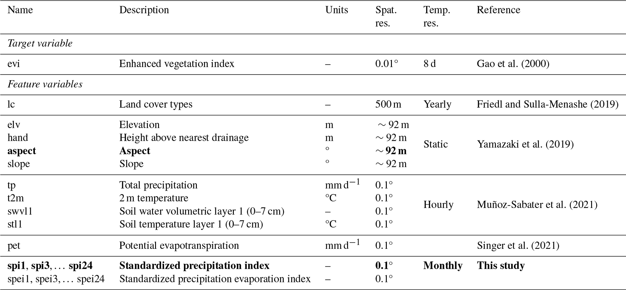
Bold text indicates that features were dropped from further analysis after conducting feature selection prior to model fitting.
Vegetation index
The reference data used in this study are the evi index values. The evi data provide an observational benchmark for the training and validation of the ML-based products created in this study. The evi can be used as an indicator of overall vegetation status and health, as it is sensitive to chlorophyll content and correlates with primary production, photosynthesis rates, and vegetation physiognomy (Box et al., 1989). Compared with the more widely used normalized difference vegetation index, the evi is considered to be the superior index, as it is less sensitive to atmospheric conditions and saturation effects in areas of dense vegetation (Gao et al., 2000). These data arise from MODIS aboard the Terra and Aqua satellites. Sensors aboard Terra and Aqua are identical, and the 16 d composite images from each sensor are released 8 d apart. In this study, Google Earth Engine's Python Application Program Interface (Gorelick et al., 2017) through the geemap package (Wu, 2020) was used to access the Terra (MOD13A2.061) and Aqua (MYD13A2.061) evi data. These two products were combined to produce a quasi-8 d time series (Didan, 2015, 2021). For the experimental setup used here, we required two sets of evi data: one at a 0.1° resolution, for training the RF and testing its gap-filling capability, and another at a 0.01° resolution, to assess the RF's downscaling abilities. To enable assessment of the gap-filling and downscaling capabilities of the RF, we downloaded one data set at a 0.01° resolution and another at a 0.1° resolution. The two different data sets (with respect to resolution) were acquired by relying on Google Earth Engines' Image Pyramiding Policy. This policy aggregates high-resolution data to the required resolution using the mean for continuous variables (i.e. evi).
Feature variables
Global vegetation dynamics are largely driven by terrestrial water and energy balances (Hawkins et al., 2003). Similarly, the responses of vegetation to drought are regulated, in part, by water and energy availability (Xu et al., 2010). Consequently, a suite of data indicative of terrestrial water and energy balances were selected as potential input variables. These variables are introduced below, and Table 1 provides an overview.
Meteorology
Hourly data for total precipitation (tp), 2 m temperature (t2m), volumetric soil moisture layer 1 (swvl1; 0–7 cm), and soil temperature layer 1 (stl1; 0–7 cm) were retrieved from the hourly ERA5-Land reanalysis product by the European Centre for Medium-Range Weather Forecasts (Muñoz-Sabater et al., 2021). In addition, potential daily evaporation (pet) was acquired from Singer et al. (2021). The pet is calculated following the Penman–Monteith formulation with ERA5-Land as the input data. This information (pet) was included because it is directly correlated with air temperature and radiation (Thornthwaite, 1948; Monteith, 1965; Priestley and Taylor, 1972) as well as with the photosynthesis potential of plants; thus, it can account for a number of other variables. All meteorological data were resampled to match the 8 d frequency of the evi data. The tp was aggregated by taking the cumulative sum of the previous 8 d, whereas the remainder of the variables were averaged over a previous 8 d window.
Drought indices
Aside from short-term changes in water availability, it is also imperative to understand the long-term dynamics to identify drought legacy effects on the current vegetation states (Schwalm et al., 2017). To this end, the standardized precipitation index (spi) (McKee et al., 1993) and standardized precipitation evapotranspiration index (spei) (Vicente-Serrano et al., 2010) were used to characterize these legacy effects. The spi and spei were calculated at 1-, 3-, 6-, 9-, 12-, and 24-month aggregation lengths. The different lengths of aggregation are related to types of drought: precipitation, soil moisture, and hydrological droughts. Precipitation and soil moisture droughts are mostly associated with short-term soil water deficits (1–3 months), and they are important for vegetation with shallow roots; hydrological drought (6–12 months) can be a good proxy for impacts on shrubs, bushes, and trees that have deeper roots and are likely to rely on local groundwater for water (12–24 months). In addition, the inclusion of drought indices allows for the characterization of past climate memory effects on current vegetation growth (Reichstein et al., 2019; Schwalm et al., 2017) associated with past climatic conditions. The equations and steps for calculating the spi and spei are detailed in Appendix A2.
Land cover types and topography
Land cover type is an important predictor of vegetation abundance and health (Meza et al., 2020). Here, the MODIS yearly Land Cover Type (MCD12Q1.061) data were retrieved from the Google Earth Engine. In this product, land cover types are classified according to the International Geosphere–Biosphere Programme classification scheme. Barren land, deserts, permanent snow, and water bodies are masked in all further analyses. It is important to note that the RF was supplied with the remaining 15 unique land cover types; however, these are collapsed into eight broader classifications for brevity and clarity in the results, discussion, and visualizations. Grasslands, wetlands, croplands, urban, and mixed did not require grouping, and they represent the corresponding classes in accordance with the Geosphere–Biosphere Programme classification scheme. Forests refers to the grouped class that contains evergreen needleleaf, evergreen broadleaf, deciduous needleleaf, deciduous broadleaf, and mixed broadleaf forests. Shrubland refers to the grouped class containing closed and open shrubland, whereas savannas refer to the grouped class containing woody savannas and savannas. To capture the variations in water and energy availability attributable to topographic effects, elevation (elv) and height from the nearest drainage basin (hand) were accessed using MERIT Hydro, a high-resolution global hydrography map (Yamazaki et al., 2019), also through Google Earth Engine. To enable assessment of the gap-filling and downscaling capabilities of the RF, we downloaded one data set at a 0.1° resolution and another at a 0.01° resolution using the Google Earth Engine's Python Application Program Interface (Gorelick et al., 2017) via the geemap package (Wu, 2020). The two different data sets (with respect to resolution) were acquired by relying on Google Earth Engines' Image Pyramiding Policy. This policy aggregates high-resolution data to the required resolution using the mode for land cover data and mean for continuous variables (i.e. evi and hand). Last, 0.1° and 0.01° slope and aspect were calculated from elv using the relevant functions in xarray-spatial (Hoyer and Hamman, 2017).
2.1.2 Random forest model
While an abundance of ML approaches have been used to predict vegetation status, here the Random forest (RF) regressor was selected to link meteorology, land cover, topography, and drought inputs to vegetation health. RF is an ensemble method that fits many decision trees on different subsets of data.
RF is advantageous given its relatively straightforward implementation, ability to incorporate categorical features, ability to easily identify causal links, and limited risk of overfitting. The general pipeline used throughout consisted of five sequential steps (Fig. 1). Here, the RF was implemented in Python 3.9 (Rossum and Drake, 2010) under the scikit-learn framework (Pedregosa et al., 2011).

Feature selection
In an attempt to include only relevant data in the ML model, the potential variables described in Sect. 2.1.1 and listed in Table 1 were evaluated with respect to their ability to provide meaningful information during model fitting. A pairwise Spearman rank correlation was calculated between all features to ensure that input data correlated with evi. Those variables that exhibited strong correlations were retained in further analysis, whereas variables that experienced weak correlations were excluded. Aspect did not exhibit strong correlations with evi (Fig. A1). Similarly, spi (at all aggregation times) did not correlate strongly with evi. In addition, spi was closely correlated with spei; thus, spi was excluded in favour of spei (Fig. A1). spi and aspect were excluded from further analyses; features that were excluded are highlighted in Table 1. Soil moisture and total precipitation exhibited some degree of cross-correlation in the global sense, yet these were retained to account for regions in which soil moisture is independent of precipitation, such as wetlands and groundwater-dependent ecosystems.
Preprocessing
Given that the RF algorithm accepts 2-dimensional numeric arrays as input, the 3-dimensional data were processed so that each unique latitude and longitude combination was associated with a time series of each variable. The single categorical feature (lc) was converted to a binary numeric form. Each unique land cover type is assigned to a new feature, with 1 indicating presence and 0 indicating absence.
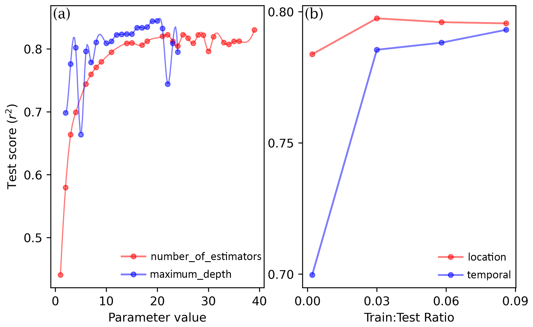
Figure 2(a) Evolution of RF performance during HalvingRandomSearchCV hyperparameter optimization of maximum_depth and number_of_estimators. (b) RF performance following the incremental increase in the training set size using a location-based split approach compared with a temporally based split approach.
Split strategy and hyperparameter optimization
To refine the number of estimators and maximum depth, a 3-fold cross-validation approach using HalvingRandomSearchCV was applied. This hyperparameter optimization provides the optimal configuration for the RF so that the critical vegetation dynamics are captured while simultaneously reducing the RF complexity and preventing overfitting. The hyperparameter optimization focused on two parameter settings, namely, maximum_depth and the number_of_estimators. The maximum_depth determines the maximum depth of the decision tree, whereas the number_of_estimators determines the number of decision trees used. The search space used for the number_of_estimators and maximum_depth was 1–40 and 1–25, respectively. The upper bounds of the search space were largely determined by computational considerations, increasing the upper limits beyond 40 for number_of_estimators and beyond 25 for maximum_depth would result in impractical computation times. Nonetheless, even with this constraint, increasing the maximum_depth and number_of_estimators past 12 and 13, respectively, yielded only marginal increases in test scores (Fig. 2a). Given that the risk of overfitting and a longer computational time increases with increasing maximum_depth and number_of_estimators as well as the fact that only marginal increases in test scores are observed past 12 and 13, these values were identified as optimal for maximum_depth and number_of_estimators, respectively.
After determining optimal parameter settings, the data were split into training and validation sets. However, 3-dimensional data could conceivably be split along the temporal dimension, where the model is trained on all locations with only a subset of the temporal availability (i.e. temporal splitting), or the data could be split according to location, where only a subset of the grid pixels are selected for training but over the entire available period (i.e. spatial splitting). Given that previous research has highlighted that RF performance is sensitive to spatial vs. temporal splitting, this is especially true for extreme events such as droughts (Hauswirth et al., 2021). We conducted a cursory analysis to determine whether a temporal or spatial splitting approach better balanced trade-offs between computational complexity and learning rates. Learning curves for cursory RF models using each splitting approach were quantified and compared. Each model was supplied with increasing training sizes, and test scores were calculated and plotted to visualize learning curves. This cursory analysis revealed that spatial splitting yields faster learning curves than the temporal splitting approach (Fig. 2b); therefore, spatial splitting was identified as the preferred approach.
Training
For the final RF model, a spatial split with a 0.06:0.94 (train : predict) ratio was used to train the final model. A 0.06:0.94 split was chosen, as there was very little increase in performance past training sizes of 6 % (Fig. 2b). The maximum_depth and number_of_estimators were set at 12 and 13, respectively. The parameters that were not subjected to hyperparameter optimization were set as follows: the squared_error criterion was used to measure the quality of the splits in branches; the maximum number_of_features considered in each split was set to auto, which instructs the algorithm to consider all features when considering a split; the minimum samples_per_leaf_node, which determines the minimum number of samples required in a leaf node, was set at the default value of 1; and the minimum samples_per_split was also set at the default value of 2, which means a split will only be considered if each branch left and right of an internal node has at least two samples in it.
2.2 Gap filling evi using random forests
As a test of the RF gap-filling capabilities, we predicted evi for the 94 % of grid cells not used during training. The accuracy of these predictions was evaluated against the evi data obtained from MODIS. As a first-pass assessment of overall performance, the model was scored using a default coefficient of determination (R2) scorer in the RF implementation of scikit. The model predictions were further evaluated by calculating the root-mean-square error (RMSE) and the Pearson correlation coefficient. These were calculated independently for each grid cell to provide information on the spatial variation in errors. Last, to gain insight into which features were the most essential for predicting evi, global feature importance was calculated using the Shapley Additive exPlanations (SHAP) TreeExplainer (Lundberg et al., 2020).
2.3 Downscaling the evi using random forests
In this section, the focus shifts toward whether RF can be used to downscale global evi values – that is, whether a model trained on 0.1° resolution data can accurately predict evi at a finer 0.01° scale. To this end, a 0.01° resolution data set was compiled. In cases where data were not at a 0.01° resolution (i.e. meteorology and drought indices data), the nearest-neighbour interpolation scheme from xarray (Hoyer and Hamman, 2017) was used to match the variables to the same spatial resolution. This data set was used as new input data for the already trained RF model to predict evi at a 0.01° scale. The evaluation approach for the downscaled values remained much the same: the overall model accuracy was assessed using the R2 and RMSE, and Pearson correlation coefficients were calculated for each grid cell.
2.4 Applicability of ML-informed vegetation status products during periods of drought
One noticeable shortcoming of the RF is its relatively poor ability to predict extreme values depending on the training selection (Hauswirth et al., 2021). To determine the extent to which this may influence the generality of the two products mentioned above, we further investigated the accuracy of the predicted evi under low growing conditions by calculating the anomaly correlation coefficient of the evi (eviACC; Eq. 1):
where eviACCi,j denotes the evi anomaly for the month j in year i, denotes the average evi of month j over 2003–2013, and σ stands for the standard deviation of evi during the period. We use this metric to assess the applicability of the RF-based 0.1 and 0.01° evi predictions against remotely sensed evi. We consider eviACC values greater than 0 as capable of capturing anomalies beyond the seasonal cycle and values exceeding 0.2 as good, given the strong seasonal cycle that is present in evi data.
Here, the results are presented in three parts. First, the results of the model trained on the 0.1° resolution data are presented; the focus is on the model's performance and ability to predict the status of the vegetation at the spatial resolution that it was not trained at, thereby assessing its ability as a gap-filling tool. We also touch on which features are most important for predicting the status of the vegetation. Subsequently, we present the model's performance when used to downscale the evi and predict 0.01° resolution data. Last, we explore how this model can be used to gain insight into global vegetation dynamics by assessing the accuracy of both products under drought conditions.
3.1 Gap filling the evi using random forests
The model was able to reproduce global vegetation patterns by correctly predicting high vegetation density in tropical forests and low vegetation density in arid and urban regions of the world (Fig. 3). SHAP values provided an understanding of the relative importance of each feature with respect to predicting evi. The most important features were those associated with meteorology, land cover type, and elevation; drought indices and slope proved to be less important (Fig. 4).
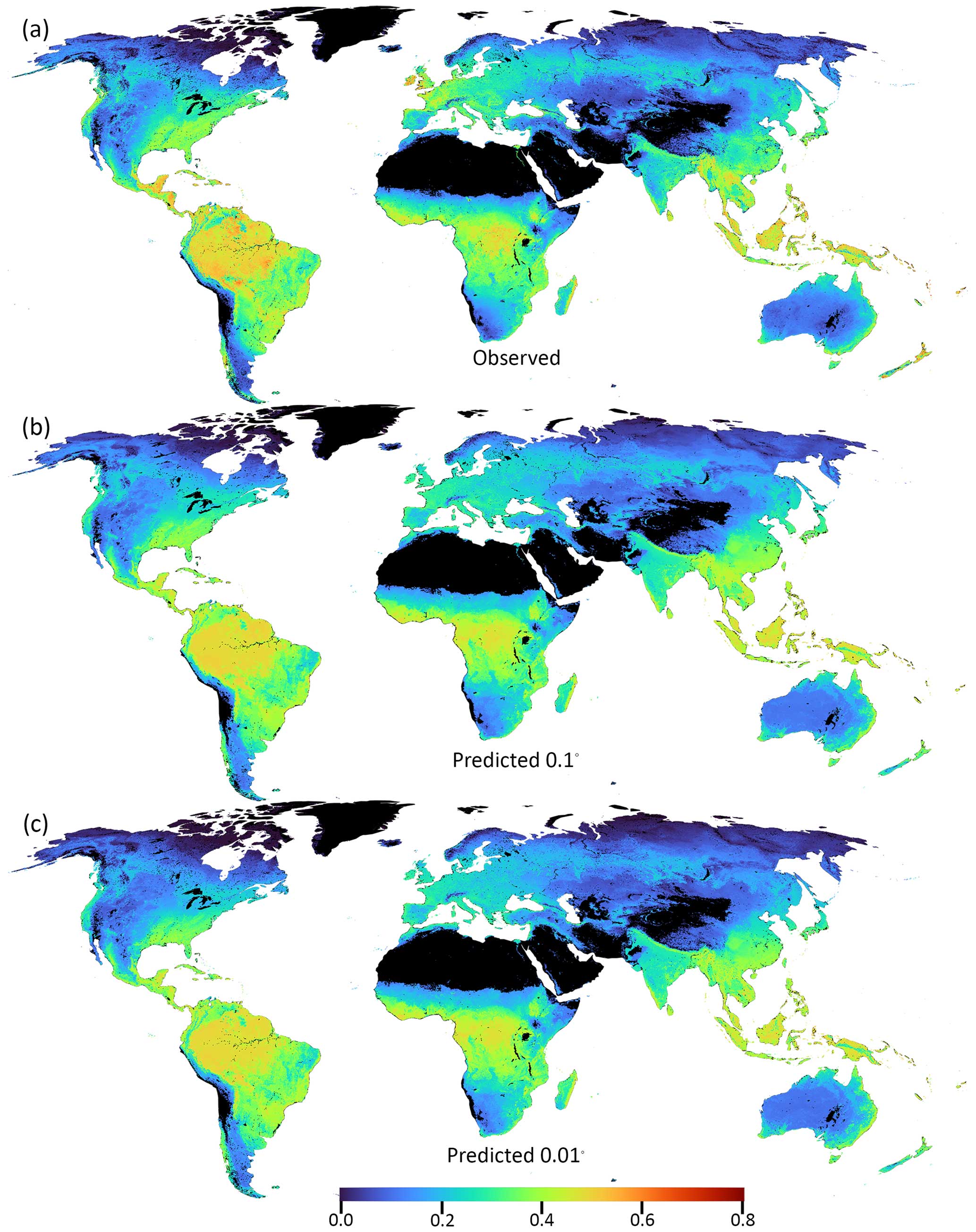
Figure 3Mean evi (2003–2013) for the (a) observed, (b) predicted 0.1°, and (c) predicted 0.01° values by the RF. Barren land, deserts, permanent snow, and water bodies were masked and are represented using black.
When trained on only 6 % of the data (i.e. the point at which the use of additional data did not result in better predictions but increased the risk of overfitting), the RF was able to predict the global evi accurately with a spatial resolution of 0.1° (R2=0.86; Figs. 3–6 and 7a). Looking more closely at the distribution of errors, less than 1 % of grid cells showed negative correlations, more than 80 % showed correlations higher than 0.5 (Fig. 7c), and the RMSE ranged between 0.02 and 0.4 (mean: 0.05±0.03; Fig. 7d). However, it is important to note that the accuracy was neither spatially nor temporally uniform. Land cover types were an important feature in determining predictive ability. The evi predictions in areas dominated by urban, mixed, and crop land cover types showed the highest degree of error (Fig. 6a). On the contrary, the most natural types of land cover, such as forests and grasslands, were the most accurately represented by the model (Figs. 5a and 6a). For all types of land cover, the periods of maximum and minimum evi were less accurately predicted than the intermediate periods (Fig. 6a). Predicted evi was consistently overestimated by the model for urban land covers (Fig. 6a).
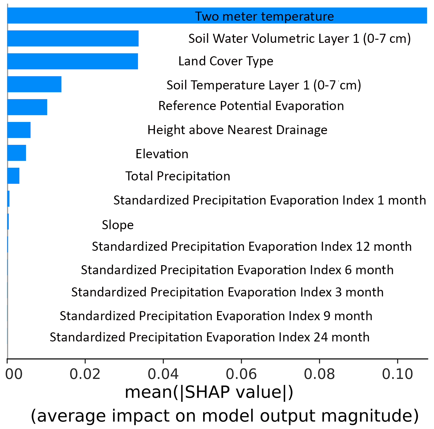
Figure 4Feature importance for the RF-based predicted evi at a 0.1° resolution. The features are ordered by level of importance, with higher mean SHAP values indicating higher importance.
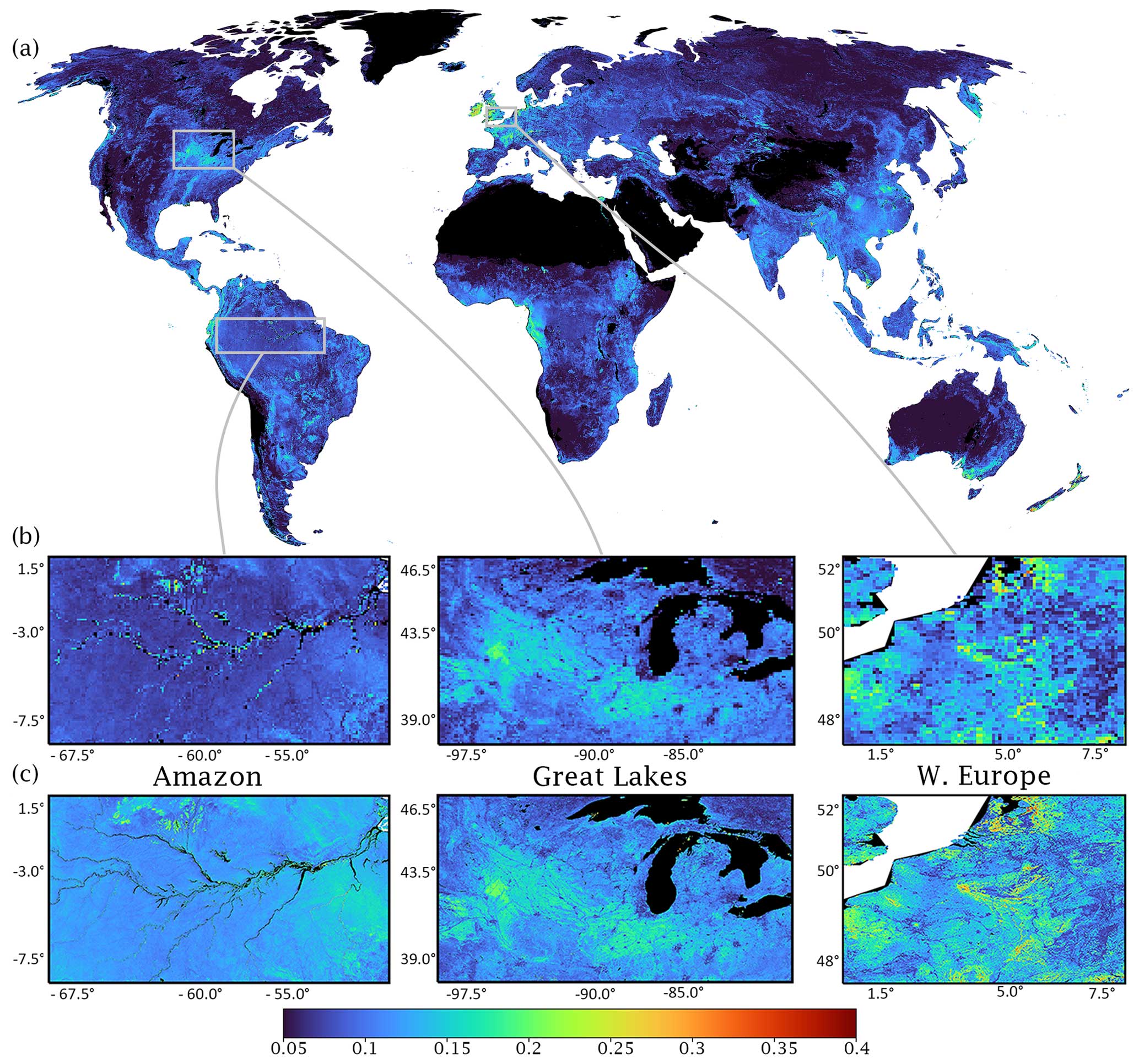
Figure 5(a) RMSE for the RF-predicted evi. The close-up inset panels show the Amazon Basin as representative region for forest land cover, the Great Lakes as a representative region for croplands, and western Europe as a representative region for urban land cover at (b) 0.1° and (c) 0.01° resolutions.
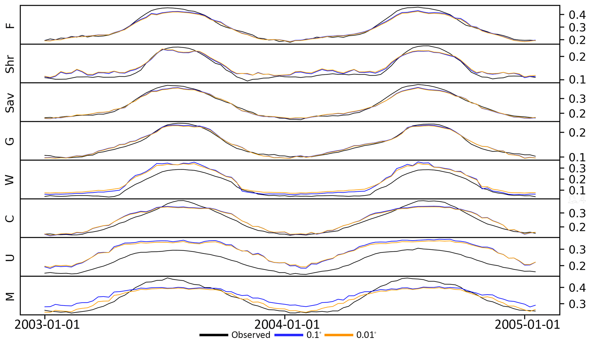
Figure 6Time series of the average and predicted evi per major land cover type at 0.1° and 0.01° resolutions. The abbreviations on the y axis are as follows: F – forest; Shr – shrubland; Sav – savanna; G – grassland; W – wetlands; C – crops; U – urban; M – mixed.
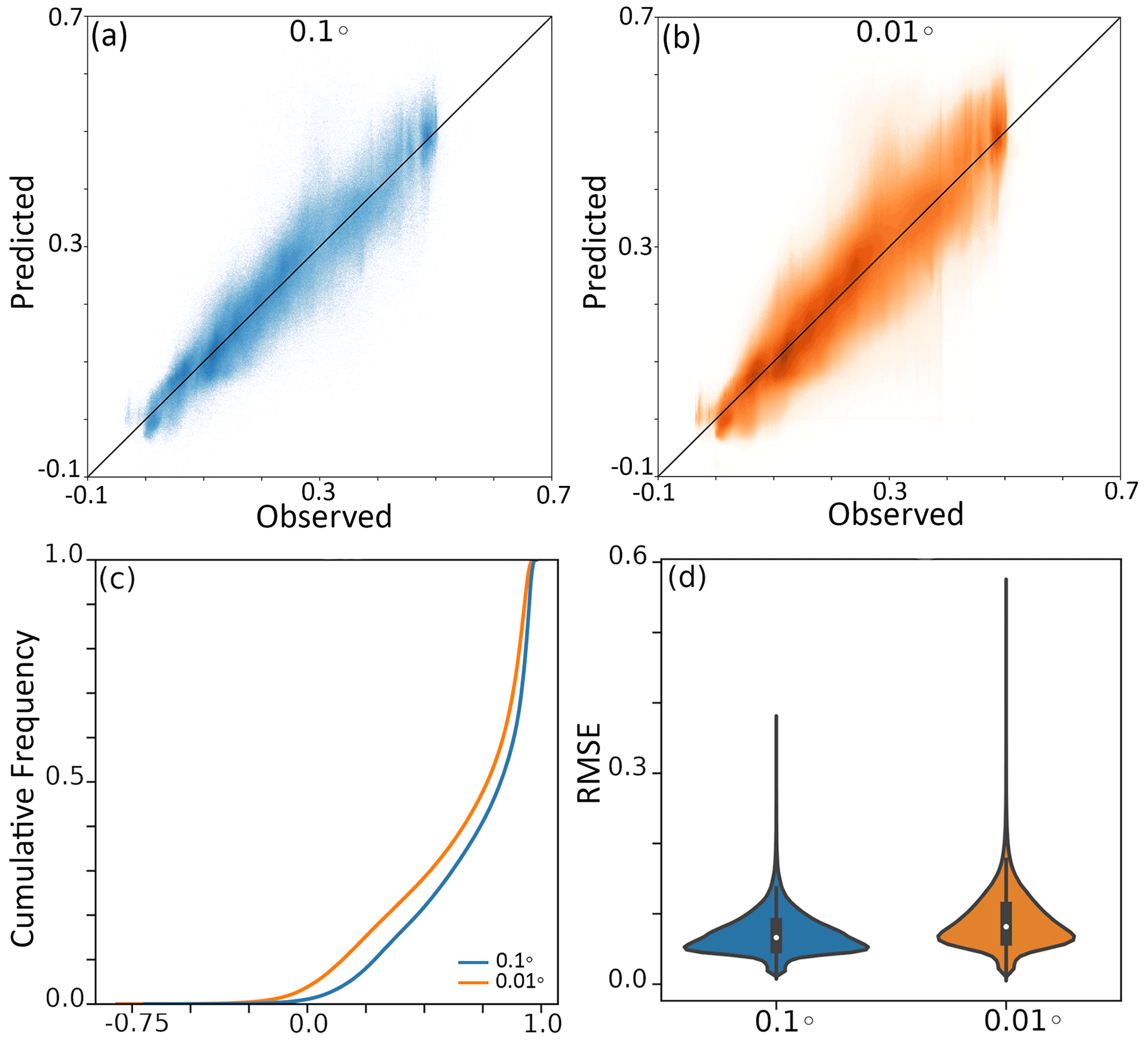
Figure 7Scatterplot of the observed and predicted evi at (a) 0.1° and (b) 0.01° resolutions; cumulative distribution function for (c) Pearson correlation coefficients for all grid points at 0.1° and 0.01° resolutions; (d) violin plot of the RMSE for all grid points at 0.1° and 0.01° resolutions.
3.2 Downscaling the evi using random forests
When the model trained on 0.1° data was used to predict evi at the 0.01° spatial resolution, there was a slight drop in accuracy, but the model was still able to capture spatial and temporal vegetation dynamics when supplied with 0.01° data (Figs. 5 and 7b). The predictive capacity was still good, although reduced compared with the 0.1° product, with a median R2 of 0.75 (Fig. 7b). The errors also increased: 5 % of grid cells displaying negative correlations (Fig. 7c) compared with less than 1 % for the 0.1° product. The RMSE ranged between 0.04 and 0.6 (mean: 0.09±0.07; Fig. 7d), with the majority of the grid cells exhibiting an RMSE of around 0.05. Accuracy was again dependent on the land cover, with urban, mixed, and crop land cover types performing the worst (Fig. 6b). Noticeably, the model consistently overestimated the evi for urban land cover types.
3.3 Accuracy under drought conditions
The anomaly correlation analysis revealed that the RF was still able to capture evi anomalies (Fig. 8), although to a lesser extent compared with overall performance (Fig. 7c). The majority of grid cells showed positive correlations, with less than 10 % displaying negative correlations; indicating that, for that 90 % of the locations where eviACC was positive, the RF can reproduce anomalies from the average seasonal cycle and, thus, be used to identify periods of negative or positive evi impacts resulting from droughts or more favourable growing conditions. More than 50 % of grid cells exhibited an eviACC of 0.25 for 0.1° resolution data compared with 45 % when the evi was predicted at a 0.01° resolution (Fig. 8).
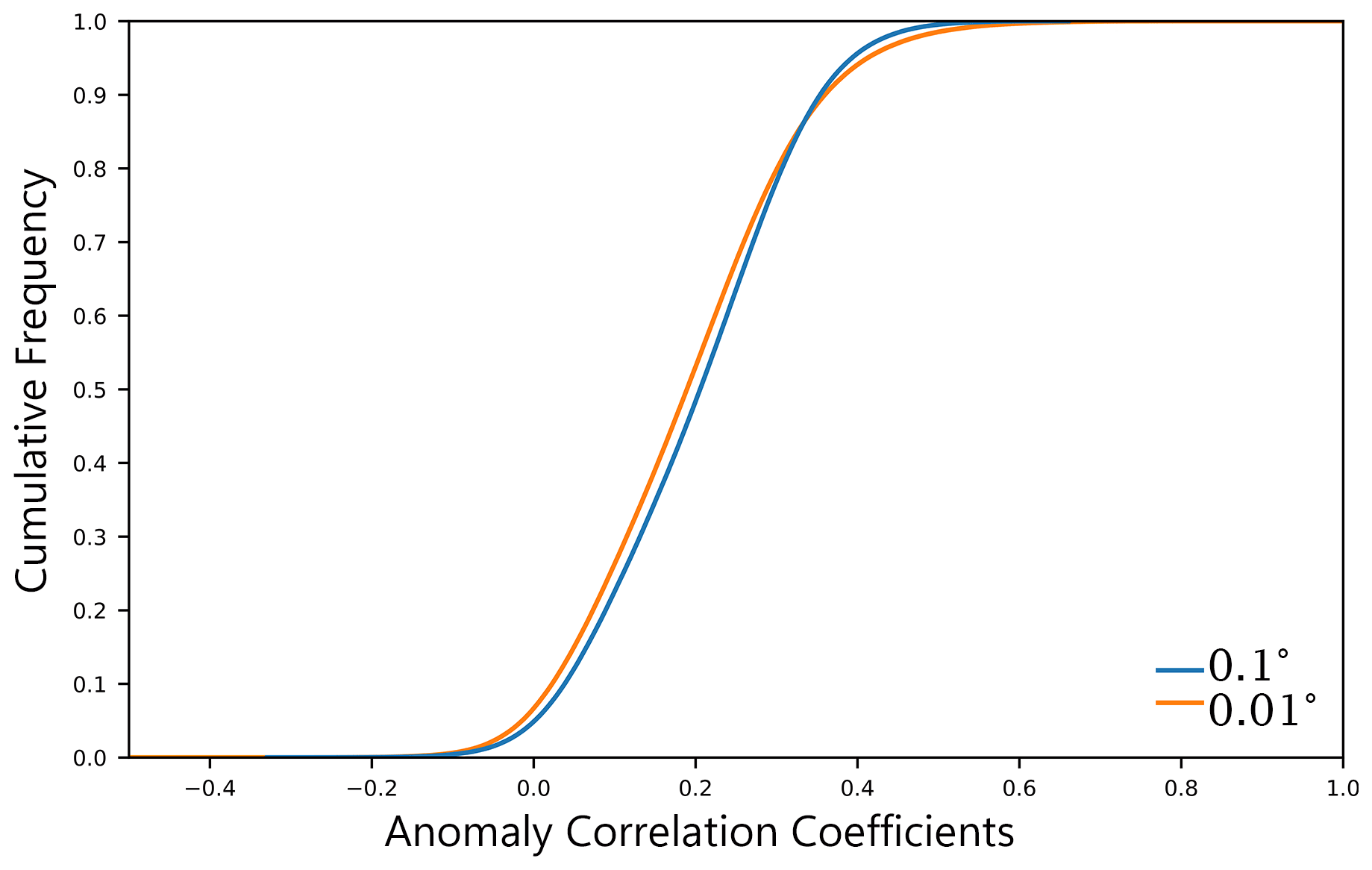
Figure 8Cumulative distribution curves of anomaly correlation coefficients for the evi predicted using RF at a 0.1° resolution (blue) and 0.01° resolution (orange).
4.1 Gap filling the evi using random forests
Here, the results show that RF can accurately predict the evi at unseen geographic locations when trained on relatively few data; in this work, training the RF on only 6 % of data provides a representative sample of the global distribution of evi values (see Sect. 4.4 for further discussion on the influence of data representativity). Using RF as a gap-filling tool has previously been applied to remotely sensed vegetation indices (Roy, 2021; Sarafanov et al., 2020; Sun et al., 2023; Wang et al., 2021; Moreno-Martínez et al., 2018), albeit mostly at a more local scale. Although it is challenging to directly compare the errors in a global product to other regional products, the errors and correlations reported here are comparable with regional studies (R2: ≈0.9; RMSE: 0.02–0.4). Two previous studies have, however, applied ML techniques to predict the evi at a global scale. These studies relied on long short-term memory (LSTM) networks, using only meteorological input data, to predict the global 15 and 8 d evi at a 0.5° (Chen et al., 2021) and 250 m (Xiong et al., 2023) resolution, respectively. This study, using a more simple ML model, reports similar rates of error (R2: ≈0.9; RMSE: 0.02–0.4) compared with the more sophisticated methods in Chen et al. (2021) (RMSE: 0.01) and Xiong et al. (2023) (R2: ≈0.9; RMSE: ≈ 0.07); this suggests that using multiple sources of input data is beneficial. The use of multiple sources of Earth data in conjunction with RF has also been employed for predicting global soil moisture (L. Zhang et al., 2021). In addition to other ML-based methods, this current work adds to the number of existing available tools (reviewed in Peng et al., 2017) that can be used for gap filling and the production of global and spatially continuous evi data sets.
4.2 Downscaling the evi using random forests
The RF accurately predicted the evi at finer spatial scales than those used to train the model, successfully predicting the evi at a scale of 0.01° using high-resolution auxiliary data. However, it should be noted that this resulted in a reduction in precision compared with the 0.1° product. This is an expected result, given that the evi at a 0.01° resolution will exhibit greater variances and more extreme values during periods of high and low growth. Scale-dependent drivers of vegetation dynamics may be another phenomenon that contributes to decreased precision when predicting the evi at a 0.01° resolution using a model trained at a coarser resolution. Meteorology has been shown to be tightly coupled to vegetation at the ecosystem scale but less so at finer scales, where biotic processes, such as competition, herbivory, disease, and fire, are more important (Franklin et al., 2020). When predicting the evi, the relative increases in error remained small. Vegetation indices downscaled using ML methods have been applied to downscale other remotely sensed variables, such as precipitation (Park et al., 2022), evapotranspiration (Hobeichi et al., 2023), and gross primary productivity (Gensheimer et al., 2022).
4.3 Random forests for predicting drought effects
The increase in error among extreme values is a known limitation of RF (Hauswirth et al., 2021); thus, RF was less capable of capturing extreme evi values compared with the overall performance of the model. During RF training, an evaluation metric, in this case squared_error, is used to minimize the error for the model as a whole. In this scenario, optimal fits inevitably result in reduced errors for values close to the mean at the expense of inflated errors for the outliers (Ribeiro and Moniz, 2020). In the current study, this means that the evi during normal growth periods is prioritized over periods of extremely low or high vegetation growth. Nonetheless, given that the majority of the grid cells exhibited positive anomaly correlations, the ability to predict the vegetation status under drought is still a positive result, in accordance with previous research (Prodhan et al., 2022; Hauswirth et al., 2021). As more sophisticated ML models tend to predict extreme values more accurately than the RF model used here (e.g. Kladny et al., 2024), future studies should aim to evaluate their feasibility and applicability to predict vegetation status under drought conditions at the global scale. However, in comparison with RF, the more complex algorithms have larger computational requirements during model training and are less capable of capturing potential nonlinearities.
4.4 Importance of land cover type and input data
Varying error according to land cover type at the 0.1° and 0.01° resolutions is expected for at least two reasons: the first relates to the inherent features of the RF algorithm itself, while the second relates to the environmental process that affects the dynamics of the evi. A limitation of the RF algorithm is that underrepresented groups are less well explained by the algorithm when data are imbalanced. Accordingly, accuracy varied according to a proportional abundance of land cover types (Jung et al., 2020). Dominant land cover types, such as forests and grasslands, displayed the least amount of error; in contrast, minority land cover types, such as regions that have undergone human modification (i.e. urban areas and croplands), were associated with the highest error. Moreover, the features used in this study may not equally incorporate processes critical to vegetation status among land cover types (Moussa Kourouma et al., 2021). Forests, grasslands, and other natural ecosystems are closely coupled to water availability determined by climatic variation processes. However, croplands and urban areas may be less influenced by weather and more influenced by anthropogenic manipulations of water and energy balances (Zhang et al., 2004; Hawkins et al., 2003; Tang et al., 2021). A potential solution to this problem is to rely on extreme gradient boosting decision trees, which have been shown to provide more accurate predictions when data are imbalanced (X. Li et al., 2021) or include information on anthropogenic water management, to better represent drought responses (Wanders and Wada, 2015).
Land-cover-specific variations in the model’s ability to predict vegetation are an important outcome of this study. Apart from the statistical reasons detailed as potential mechanisms for this phenomenon in the previous paragraph, an additional, and most likely compounding, explanation is that the data used to predict the evi may be more relevant for some land cover types and levels of vegetation growth than others. For instance, vegetation status in urban areas and croplands shows weak correlation or high errors (Figs. 5 and 6). The meteorological data used here to predict the evi may not be the only factor driving the vegetation dynamics in anthropogenically modified areas. It is possible that irrigation, harvesting, and water management influence vegetation. Indeed, vegetation in urban areas has been shown to grow more rapidly and have a longer growing season compared with rural regions; this is thought to be driven by higher temperatures and by a high concentration of airborne phosphorous and other aerosol pollutants (Sicard et al., 2018a, b; Pretzsch et al., 2017). In contrast, natural forests and grasslands show high levels of accuracy and correlations, suggesting that the data used here are appropriate for the ML models to capture vegetation dynamics. Similarly, poor accuracy in wetlands is not unexpected, as wetland vegetation is primarily driven by water quality, salinity, and pH (Grieger et al., 2021). On the contrary, forests and grasslands show high accuracy when using meteorological variables, as these are important drivers of vegetation growth in these areas. Although not directly related to vegetation, Hauswirth et al. (2021) showed that the inclusion of water management practices in ML models resulted in more accurate predictions of groundwater head flow and streamflow. It is important to note that the relevancy of predictors in shaping the evi does not only affect the accuracy between land cover types but also plays a role in determining the overall accuracy of the model. For instance, precipitation and soil moisture do not exhibit similar feature importance, whereas soil temperature and 2 m temperature do. The amount of precipitation retained in soils is dependent on a number of factors, and these results suggest that soil water moisture is a more critical variable than precipitation in governing the global evi dynamics; this aligns with observation of soil precipitated water residence times that are often much longer than the actual precipitation events (McColl et al., 2017). In addition, slope is known to be an important determinant of vegetation status at fine spatial resolutions (Chen et al., 2013). However, the relatively weak feature importance of slope suggests that the model could not find much meaningful information regarding vegetation status and slope at a 0.1° resolution during training and, subsequently, would be unable to use this information when predicting the evi at a 0.01° resolution.
One other possibility is that uncertainty in the input data prevents more accurate predictions by the model. The temperature of ERA5-Land is known to show weaker correlations with observed data in the tropics compared with more northern and southern latitudes (Muñoz-Sabater et al., 2021). In accordance with that, the errors in the evi predicted using the RF model largely follow this pattern: errors are higher in the tropics compared with the temperate zones. The temperature from ERA5-Land shows relatively higher errors along the Andes, the northern reaches of the African rainforest, and the Sichuan Basin in China, and the errors in predicted evi mirror this uncertainty. Similarly, when comparing errors in the soil water content from ERA5-Land, Gabon forest's, the Andes, Vietnam, New South Wales in Australia, and the East African Rift system have relatively high errors (Lal et al., 2022). Again, the errors in the predicted evi are also relatively high in these regions. When considering the quality of land cover data used here, some inconsistencies may affect the ability of the RF to accurately predict the evi. For example, when croplands are smaller than the pixel size used in MODIS, these areas are incorrectly assigned as natural vegetation. Furthermore, temperate evergreen needleleaf forests are misclassified as broadleaf evergreen forests, and some grassland areas are classified as savannas. The relatively poor predictive performance in mixed land cover types further reiterates the need to provide models with appropriate input data sources where string signals are present. In addition, data that are more relevant to vegetation dynamics could provide better results; for example, the weak feature importance of slope and the various spei metrics at their various aggregation times suggests that these variables do not play a relatively important role predicting the evi at the temporal and spatial scales here. By way of illustration, at fine scales, slope and aspect are important for determining radiation intensity experienced by plants, but training the model at a 0.1° resolution means that this effect becomes less important and is not learnt by the model. Perhaps a better result would be acquired if more scalable variables were included, specifically for the downscaling component.
The results of this study reveal that RF is an appropriate method for predicting the evi at the global scale, at a 0.1° resolution and downscaled 0.01° resolution. In general, RF was capable of predicting evi dynamics with high accuracy; global patterns of vegetation and temporal dynamics were well captured by land cover, with variables relating to the energy and water balances experienced by plants having the most significance. The model was able to capture annual vegetation growth cycles and distinguish between the main global biomes with high accuracy. However, it is essential to note that higher errors were associated with underrepresented land cover types and periods of extreme vegetation growth, such a drought periods. Lower accuracy for underrepresented classes in unbalanced data sets and a hampered ability to predict extreme values are common criticisms of RF. In accordance with this study, land cover types that account for a smaller fractional cover of the Earth's surface and periods of extreme vegetation growth were associated with the highest error. Predicting the evi at a finer resolution resulted in increased errors. This is attributed to higher variances in the 0.01° product compared with the 0.1° product, although it is important to note that the relative increases remained small.
The results here also highlight the use of RF for efficiently and accurately predicting missing data and downscaling, ultimately allowing for the production of spatially continuous evi data sets at very high spatial and temporal resolutions. To this end, this study produces a spatially continuous evi product at 0.1° and 0.01° resolutions; therefore, this approach could be used to fill existing gaps in satellite observations or in conjunction with satellite data to improve the monitoring of drought impacts on vegetation. For example, the Landsat and Sentinel-2 satellites can produce high-resolution vegetation products; however, retrievals are strongly affected by weather conditions, resulting in data gaps. In addition, the satellites' relatively low orbiting altitude means that the spatial coverage for each overpass is low. Using this approach on such data could produce globally continuous vegetation products at spatial resolutions lower than 100 m.
This study shows that ML can be used for drought monitoring at high spatial and temporal resolutions; however, there are trade-offs when it comes to using ML for vegetation drought impact monitoring. ML-based evi estimates can be used to assess the potential impact of droughts on vegetation, but these estimates still require a meteorological input data set. The ML model also needs to be trained on actual remotely sensed evi observations to identify the relationship between these meteorological variables and vegetation drought impacts. This inherently makes the ML-based estimates as good as the remotely sensed product; therefore, as long as no reliable alternative exists, it will be difficult to fully replace remotely sensed evi observations. However, there is an added benefit of having continuous high-resolution global coverage derived from an ML-based evi estimate. Finally, the ML-based estimates also allow us to extrapolate the evi records to historical periods for which meteorological data exist but satellite remotely sensing was not yet available or for use as post-processing in hydrological model simulations to directly estimate drought impacts.
This study adds to previous research efforts that have successfully applied RF to predict the vegetation status. Here, RF was used to produce a global, spatial and temporally continuous evi product at 0.1° and 0.01° resolutions, with a median R2 of 0.86 and 0.75, respectively. The approach outlined in this study could be applied to Landsat and Sentinel-2 to produce continuous vegetation index data sets at a 30–10 m spatial resolution. The RF algorithm is a powerful technique for predicting temporal and spatial vegetation dynamics from remote-sensing data and can be used for gap filling and downscaling. The novelty of this product, compared with previous studies, is that it has global coverage and high spatial and temporal resolution.
A1 Feature selection
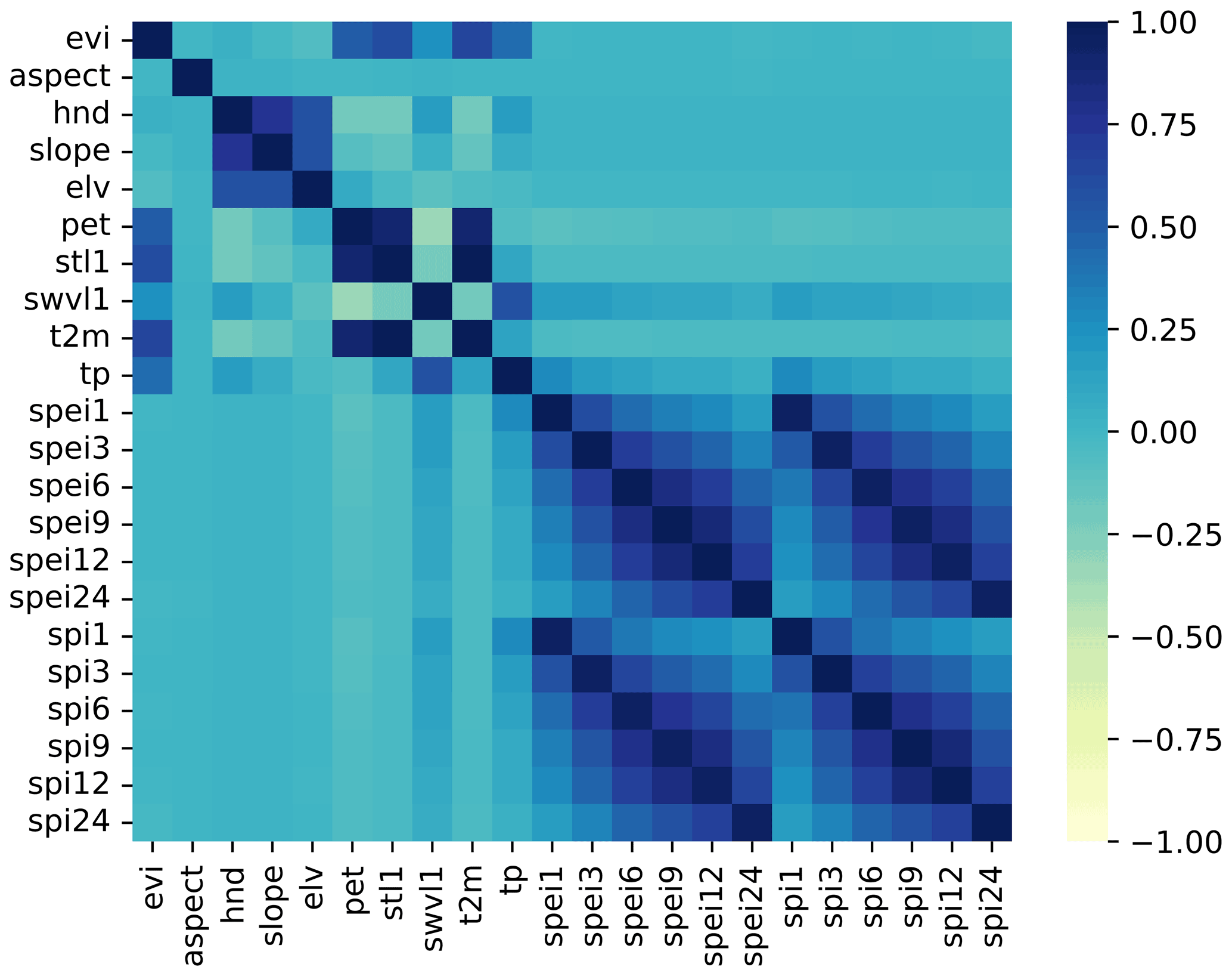
Figure A1Correlation matrix of pairwise Spearman rank correlation coefficients between all potential variables.
A2 Drought indices calculations
For the calculation of spi, we utilized the following expression:
where i is the month in question and .
For the calculation of spei, we utilized the following expression:
where and
This time series is then fitted to a gamma distribution, using the following steps. First, the α and β fitting parameters are calculated as follows:
where (with n being number of observations), and
The gamma distribution probability density (Eq. A6) function with respect to x and including the calculated estimates for α and β can be inserted to produce an equation for the cumulative probability of a value for (Eq. A7)
where α is the shape parameter, β is the scale parameter, and .
Then, substituting t for results in the incomplete gamma distribution (Eq. A8):
Values of the incomplete gamma function can be computed using the following expression:
Finally, values computed from Eq. (A9) are transformed into the standard normal distribution to yield the spi and spei at the relevant timescales. These calculations were completed using the relevant algorithms in the climate_indices Python package (Adams, 2017) using tp, pet, and t2m, as detailed in Sect. 2.1.2.
Google Earth Engine was used to acquire the enhanced vegetation index (https://doi.org/10.5067/MODIS/MYD13A2.061, Didan, 2015), land cover (https://doi.org/10.5067/MODIS/MCD12C1.061, USGS, 2024), and hydrography (elv, hand, aspect, and slope; https://doi.org/10.1029/2019WR024873, Yamazaki et al., 2019) information. Meteorological data (tp, t2m, swvl1, and stl1) were obtained from the Copernicus Climate Data Store (https://doi.org/10.24381/cds.e2161bac, Muñoz-Sabater, 2019). Potential evapotranspiration was acquired from Singer et al. (2020) (https://doi.org/10.5523/bris.qb8ujazzda0s2aykkv0oq0ctp).
BvJ and SMH: data curation, formal analysis, writing – review and editing; NW: conceptualization, formal analysis, writing – review and editing.
At least one of the (co-)authors is a member of the editorial board of Hydrology and Earth System Sciences. The peer-review process was guided by an independent editor, and the authors also have no other competing interests to declare.
Publisher's note: Copernicus Publications remains neutral with regard to jurisdictional claims made in the text, published maps, institutional affiliations, or any other geographical representation in this paper. While Copernicus Publications makes every effort to include appropriate place names, the final responsibility lies with the authors.
Views and opinions expressed are those of the author(s) only and do not necessarily reflect those of the European Union or the European Research Council. Neither the European Union nor the granting authority can be held responsible for them.
Steven M. de Jong is thanked for his valuable input on previous versions of this manuscript. The authors are grateful to Oddbjørn Bruland and the three anonymous reviewers whose comments helped to improve the manuscript.
Sandra M. Hauswirth received financial support from the Cooperate Innovation Program and the Department of Water, Transport, and Environment at the Dutch National Water Authority, Rijkswaterstaat. Niko Wanders received funding from the European Union (ERC-Stg, Multi-Dry, grant no. 101075354).
This paper was edited by Thom Bogaard and reviewed by Oddbjørn Bruland and three anonymous referees.
Adams, J.: Climate Indices in Python, GitHub [code], https://github.com/monocongo/climate_indices (last access: 22 November 2022), 2017. a
AghaKouchak, A., Farahmand, A., Melton, F. S., Teixeira, J., Anderson, M. C., Wardlow, B. D., and Hain, C. R.: Remote sensing of drought: Progress, challenges and opportunities: Remote Sensing Of Drought, Rev. Geophys., 53, 452–480, https://doi.org/10.1002/2014RG000456, 2015. a, b
Banerjee, O., Bark, R., Connor, J., and Crossman, N. D.: An ecosystem services approach to estimating economic losses associated with drought, Ecol. Econ., 91, 19–27, https://doi.org/10.1016/j.ecolecon.2013.03.022, 2013. a, b
Blauhut, V., Stahl, K., Stagge, J. H., Tallaksen, L. M., De Stefano, L., and Vogt, J.: Estimating drought risk across Europe from reported drought impacts, drought indices, and vulnerability factors, Hydrol. Earth Syst. Sci., 20, 2779–2800, https://doi.org/10.5194/hess-20-2779-2016, 2016. a
Box, E. O., Holben, B. N., and Kalb, V.: Accuracy of the AVHRR vegetation index as a predictor of biomass, primary productivity and net CO2 flux, Vegetatio, 80, Springer, 71–89, https://doi.org/10.1007/BF00048034, 1989. a
Cammalleri, C., Naumann, G., Mentaschi, L., Formetta, G., Forzieri, G., Gosling, S., Bisselink, B., De Roo, A., and Feyen, L.: Global warming and drought impacts in the EU: JRC PESETA IV project: Task 7, Publications Office, LU, https://data.europa.eu/doi/10.2760/597045 (last access: 16 June 2022), 2020. a
Chen, J. M., Chen, X., and Ju, W.: Effects of vegetation heterogeneity and surface topography on spatial scaling of net primary productivity, Biogeosciences, 10, 4879–4896, https://doi.org/10.5194/bg-10-4879-2013, 2013. a
Chen, Q., Timmermans, J., Wen, W., and van Bodegom, P. M.: A multi-metric assessment of drought vulnerability across different vegetation types using high resolution remote sensing, Sci. Total Environ., 832, 154970, https://doi.org/10.1016/j.scitotenv.2022.154970, 2022. a
Chen, Z., Liu, H., Xu, C., Wu, X., Liang, B., Cao, J., and Chen, D.: Modeling vegetation greenness and its climate sensitivity with deep‐learning technology, Ecol. Evol., 11, 7335–7345, https://doi.org/10.1002/ece3.7564, 2021. a, b, c
Crausbay, S. D., Ramirez, A. R., Carter, S. L., Cross, M. S., Hall, K. R., Bathke, D. J., Betancourt, J. L., Colt, S., Cravens, A. E., Dalton, M. S., Dunham, J. B., Hay, L. E., Hayes, M. J., McEvoy, J., McNutt, C. A., Moritz, M. A., Nislow, K. H., Raheem, N., and Sanford, T.: Defining Ecological Drought for the Twenty-First Century, B. Am. Meteorol. Soc., 98, 2543–2550, https://doi.org/10.1175/BAMS-D-16-0292.1, 2017. a
Das, P., Naganna, S. R., Deka, P. C., and Pushparaj, J.: Hybrid wavelet packet machine learning approaches for drought modeling, Environ. Earth Sci., 79, 221, https://doi.org/10.1007/s12665-020-08971-y, 2020. a
Didan, K.: MOD13A2 MODIS/Terra Vegetation Indices 16-Day L3 Global 1 km SIN Grid V006, NASA EOSDIS LP DAAC [data set], https://doi.org/10.5067/MODIS/MYD13A2.061, 2015. a, b
Didan, K.: MODIS/Aqua Vegetation Indices Monthly L3 Global 0.05 Deg CMG V061, NASA EOSDIS Land Processes DAAC [data set], https://doi.org/10.5067/MODIS/MOD13A2.061, 2021. a
Ebrahimy, H., Aghighi, H., Azadbakht, M., Amani, M., Mahdavi, S., and Matkan, A. A.: Downscaling MODIS Land Surface Temperature Product Using an Adaptive Random Forest Regression Method and Google Earth Engine for a 19-Years Spatiotemporal Trend Analysis Over Iran, IEEE J. Select. Top. Appl. Earth Obs. Remote Sens., 14, 2103–2112, https://doi.org/10.1109/JSTARS.2021.3051422, 2021. a
Franklin, O., Harrison, S. P., Dewar, R., Farrior, C. E., Brännström, A., Dieckmann, U., Pietsch, S., Falster, D., Cramer, W., Loreau, M., Wang, H., Mäkelä, A., Rebel, K. T., Meron, E., Schymanski, S. J., Rovenskaya, E., Stocker, B. D., Zaehle, S., Manzoni, S., van Oijen, M., Wright, I. J., Ciais, P., van Bodegom, P. M., Peñuelas, J., Hofhansl, F., Terrer, C., Soudzilovskaia, N. A., Midgley, G., and Prentice, I. C.: Organizing principles for vegetation dynamics, Nat. Plants, 6, 444–453, https://doi.org/10.1038/s41477-020-0655-x, 2020. a
Friedl, M. and Sulla-Menashe, D.: MCD12Q1 MODIS/Terra+Aqua Land Cover Type Yearly L3 Global 500 m SIN Grid V006, USGS [data set], https://doi.org/10.5067/MODIS/MCD12Q1.006, 2019. a
Fu, R., Chen, R., Wang, C., Chen, X., Gu, H., Wang, C., Xu, B., Liu, G., and Yin, G.: Generating High-Resolution and Long-Term SPEI Dataset over Southwest China through Downscaling EEAD Product by Machine Learning, Remote Sens., 14, 1662, https://doi.org/10.3390/rs14071662, 2022. a
Gao, X., Huete, A. R., Ni, W., and Miura, T.: Optical–Biophysical Relationships of Vegetation Spectra without Background Contamination, Remote Sens. Environ., 74, 609–620, https://doi.org/10.1016/S0034-4257(00)00150-4, 2000. a, b
Gensheimer, J., Turner, A. J., Köhler, P., Frankenberg, C., and Chen, J.: A convolutional neural network for spatial downscaling of satellite-based solar-induced chlorophyll fluorescence (SIFnet), Biogeosciences, 19, 1777–1793, https://doi.org/10.5194/bg-19-1777-2022, 2022. a, b
Gorelick, N., Hancher, M., Dixon, M., Ilyushchenko, S., Thau, D., and Moore, R.: Google Earth Engine: Planetary-scale geospatial analysis for everyone, Remote Sens. Environ., 202, 18–27, https://doi.org/10.1016/j.rse.2017.06.031, 2017. a, b
Grieger, R., Capon, S. J., Hadwen, W. L., Mackey, B., Grieger, R., Capon, S. J., Hadwen, W. L., and Mackey, B.: Spatial variation and drivers of vegetation structure and composition in coastal freshwater wetlands of subtropical Australia, Mar. Freshwater Res., 72, 1746–1759, https://doi.org/10.1071/MF21023, 2021. a
Han, D., Wang, G., Liu, T., Xue, B.-L., Kuczera, G., and Xu, X.: Hydroclimatic response of evapotranspiration partitioning to prolonged droughts in semiarid grassland, J. Hydrol., 563, 766–777, https://doi.org/10.1016/j.jhydrol.2018.06.048, 2018. a
Hauswirth, S. M., Bierkens, M. F., Beijk, V., and Wanders, N.: The potential of data driven approaches for quantifying hydrological extremes, Adv. Water Resour., 155, 104017, https://doi.org/10.1016/j.advwatres.2021.104017, 2021. a, b, c, d, e, f
Hauswirth, S. M., Bierkens, M. F. P., Beijk, V., and Wanders, N.: The suitability of a seasonal ensemble hybrid framework including data-driven approaches for hydrological forecasting, Hydrol. Earth Syst. Sci., 27, 501–517, https://doi.org/10.5194/hess-27-501-2023, 2023. a
Hawkins, B. A., Field, R., Cornell, H. V., Currie, D. J., Guégan, J.-F., Kaufman, D. M., Kerr, J. T., Mittelbach, G. G., Oberdorff, T., O'Brien, E. M., Porter, E. E., and Turner, J. R. G.: Energy, water, and broad-scale geographic patterns of species richness, Ecology, 84, 3105–3117, https://doi.org/10.1890/03-8006, 2003. a, b
Hobeichi, S., Nishant, N., Shao, Y., Abramowitz, G., Pitman, A., Sherwood, S., Bishop, C., and Green, S.: Using Machine Learning to Cut the Cost of Dynamical Downscaling, Earth's Future, 11, e2022EF003291, https://doi.org/10.1029/2022EF003291, 2023. a
Hoyer, S. and Hamman, J.: xarray: N-D labeled Arrays and Datasets in Python, J. Open Res. Softw., 5, 10, https://doi.org/10.5334/jors.148, 2017. a, b
Huang, S., Tang, L., Hupy, J. P., Wang, Y., and Shao, G.: A commentary review on the use of normalized difference vegetation index (NDVI) in the era of popular remote sensing, J. Forest. Res., 32, 1–6, https://doi.org/10.1007/s11676-020-01155-1, 2021. a
Jung, M., Dahal, P. R., Butchart, S. H. M., Donald, P. F., De Lamo, X., Lesiv, M., Kapos, V., Rondinini, C., and Visconti, P.: A global map of terrestrial habitat types, Sci. Data, 7, 256, https://doi.org/10.1038/s41597-020-00599-8, 2020. a
Kladny, K.-R., Milanta, M., Mraz, O., Hufkens, K., and Stocker, B. D.: Enhanced prediction of vegetation responses to extreme drought using deep learning and Earth observation data, Ecol. Inform., 80, 102474, https://doi.org/10.1016/j.ecoinf.2024.102474, 2024. a
Lal, P., Singh, G., Das, N. N., Colliander, A., and Entekhabi, D.: Assessment of ERA5-Land Volumetric Soil Water Layer Product Using In Situ and SMAP Soil Moisture Observations, IEEE Geosci. Remote Sens. Lett., 19, 1–5, https://doi.org/10.1109/LGRS.2022.3223985, 2022. a
Li, S., Xu, L., Jing, Y., Yin, H., Li, X., and Guan, X.: High-quality vegetation index product generation: A review of NDVI time series reconstruction techniques, Int. J. Appl. Earth Obs. Geoinf., 105, 102640, https://doi.org/10.1016/j.jag.2021.102640, 2021. a, b
Li, X., Yuan, W., and Dong, W.: A Machine Learning Method for Predicting Vegetation Indices in China, Remote Sens., 13, 1147, https://doi.org/10.3390/rs13061147, 2021. a, b, c
Liu, Y., Jing, W., Wang, Q., and Xia, X.: Generating high-resolution daily soil moisture by using spatial downscaling techniques: a comparison of six machine learning algorithms, Adv. Water Resour., 141, 103601, https://doi.org/10.1016/j.advwatres.2020.103601, 2020. a, b
Lundberg, S. M., Erion, G., Chen, H., DeGrave, A., Prutkin, J. M., Nair, B., Katz, R., Himmelfarb, J., Bansal, N., and Lee, S.-I.: From local explanations to global understanding with explainable AI for trees, Nat. Mach. Intel., 2, 56–67, https://doi.org/10.1038/s42256-019-0138-9, 2020. a
McColl, K. A., Alemohammad, S. H., Akbar, R., Konings, A. G., Yueh, S., and Entekhabi, D.: The global distribution and dynamics of surface soil moisture, Nat. Geosci., 10, 100–104, https://doi.org/10.1038/ngeo2868, 2017. a
McKee, T. B., Doesken, N. J., and Kleist, J.: The relationship of drought frequency and duration to time scales, in: Proceedings of the 8th Conference on Applied Climatology, vol. 17, 17–22 January 1993, Boston, 179–183, https://climate.colostate.edu/pdfs/relationshipofdroughtfrequency.pdf (last access: 3 June 2024), 1993. a
Meza, I., Siebert, S., Döll, P., Kusche, J., Herbert, C., Eyshi Rezaei, E., Nouri, H., Gerdener, H., Popat, E., Frischen, J., Naumann, G., Vogt, J. V., Walz, Y., Sebesvari, Z., and Hagenlocher, M.: Global-scale drought risk assessment for agricultural systems, Nat. Hazards Earth Syst. Sci., 20, 695–712, https://doi.org/10.5194/nhess-20-695-2020, 2020. a
Monteith, J. L.: Evaporation and environment, Symposia of the Society for Experimental Biology, 19, 205–234, https://repository.rothamsted.ac.uk/item/8v5v7/evaporation-and-environment (last access: 16 July 2022), 1965. a
Moreno-Martínez, A., Camps-Valls, G., Kattge, J., Robinson, N., Reichstein, M., van Bodegom, P., Kramer, K., Cornelissen, J. H. C., Reich, P., Bahn, M., Niinemets, Ü., Peñuelas, J., Craine, J. M., Cerabolini, B. E. L., Minden, V., Laughlin, D. C., Sack, L., Allred, B., Baraloto, C., Byun, C., Soudzilovskaia, N. A., and Running, S. W.: A methodology to derive global maps of leaf traits using remote sensing and climate data, Remote Sens. Environ., 218, 69–88, https://doi.org/10.1016/j.rse.2018.09.006, 2018. a
Moussa Kourouma, J., Eze, E., Negash, E., Phiri, D., Vinya, R., Girma, A., and Zenebe, A.: Assessing the spatio-temporal variability of NDVI and VCI as indices of crops productivity in Ethiopia: a remote sensing approach, Geomat. Nat. Hazards Risk, 12, 2880–2903, https://doi.org/10.1080/19475705.2021.1976849, 2021. a, b
Muñoz Sabater, J.: ERA5-Land hourly data from 1950 to present, Copernicus Climate Change Service (C3S) Climate Data Store (CDS) [data set], https://doi.org/10.24381/cds.e2161bac, 2019. a
Muñoz-Sabater, J., Dutra, E., Agustí-Panareda, A., Albergel, C., Arduini, G., Balsamo, G., Boussetta, S., Choulga, M., Harrigan, S., Hersbach, H., Martens, B., Miralles, D. G., Piles, M., Rodríguez-Fernández, N. J., Zsoter, E., Buontempo, C., and Thépaut, J.-N.: ERA5-Land: a state-of-the-art global reanalysis dataset for land applications, Earth Syst. Sci. Data, 13, 4349–4383, https://doi.org/10.5194/essd-13-4349-2021, 2021. a, b, c
Naumann, G., Barbosa, P., Garrote, L., Iglesias, A., and Vogt, J.: Exploring drought vulnerability in Africa: an indicator based analysis to be used in early warning systems, Hydrol. Earth Syst. Sci., 18, 1591–1604, https://doi.org/10.5194/hess-18-1591-2014, 2014. a
Park, S., Singh, K., Nellikkattil, A., Zeller, E., Mai, T. D., and Cha, M.: Downscaling Earth System Models with Deep Learning, in: Proceedings of the 28th ACM SIGKDD Conference on Knowledge Discovery and Data Mining, ACM, Washington, D.C., USA, 3733–3742, ISBN 9781450393850, https://doi.org/10.1145/3534678.3539031, 2022. a
Pedregosa, F., Varoquaux, G., Gramfort, A., Michel, V., Thirion, B., Grisel, O., Blondel, M., Prettenhofer, P., Weiss, R., Dubourg, V., Vanderplas, J., Passos, A., Cournapeau, D., Brucher, M., Perrot, M., and Duchesnay, E.: Scikit-learn: Machine Learning in Python, J. Mach. Learn. Res., 12, 2825–2830, 2011. a
Peng, J., Loew, A., Merlin, O., and Verhoest, N. E. C.: A review of spatial downscaling of satellite remotely sensed soil moisture, Rev. Geophys., 55, 341–366, https://doi.org/10.1002/2016RG000543, 2017. a
Pretzsch, H., Biber, P., Uhl, E., Dahlhausen, J., Schütze, G., Perkins, D., Rötzer, T., Caldentey, J., Koike, T., Con, T. v., Chavanne, A., Toit, B. D., Foster, K., and Lefer, B.: Climate change accelerates growth of urban trees in metropolises worldwide, Sci. Rep., 7, 15403, https://doi.org/10.1038/s41598-017-14831-w, 2017. a
Priestley, C. H. B. and Taylor, R. J.: On the Assessment of Surface Heat Flux and Evaporation Using Large-Scale Parameters, Mon. Weather Rev., 100, 81–92, https://doi.org/10.1175/1520-0493(1972)100<0081:OTAOSH>2.3.CO;2, 1972. a
Prodhan, F. A., Zhang, J., Hasan, S. S., Pangali Sharma, T. P., and Mohana, H. P.: A review of machine learning methods for drought hazard monitoring and forecasting: Current research trends, challenges, and future research directions, Environ. Model. Softw., 149, 105327, https://doi.org/10.1016/j.envsoft.2022.105327, 2022. a
Reichstein, M., Camps-Valls, G., Stevens, B., Jung, M., Denzler, J., Carvalhais, N., and Prabhat: Deep learning and process understanding for data-driven Earth system science, Nature, 566, 195–204, https://doi.org/10.1038/s41586-019-0912-1, 2019. a, b
Ribeiro, R. P. and Moniz, N.: Imbalanced regression and extreme value prediction, Mach. Learn., 109, 1803–1835, https://doi.org/10.1007/s10994-020-05900-9, 2020. a
Rossum, G. V. and Drake, F. L.: The Python language reference, no. Pt. 2 in Python documentation manual, in: release 3.0.1 [repr.] edn., edited by: van Rossum, G. and Drake, F. L., Python Software Foundation, Hampton, NH, ISBN 9781441412690, 2010. a
Roy, B.: Optimum machine learning algorithm selection for forecasting vegetation indices: MODIS NDVI & EVI, Remote Sens. Appl.: Soc. Environ., 23, 100582, https://doi.org/10.1016/j.rsase.2021.100582, 2021. a, b, c
Sarafanov, M., Kazakov, E., Nikitin, N. O., and Kalyuzhnaya, A. V.: A Machine Learning Approach for Remote Sensing Data Gap-Filling with Open-Source Implementation: An Example Regarding Land Surface Temperature, Surface Albedo and NDVI, Remote Sens., 12, 3865, https://doi.org/10.3390/rs12233865, 2020. a
Schneider, T., Lan, S., Stuart, A., and Teixeira, J.: Earth System Modeling 2.0: A Blueprint for Models That Learn From Observations and Targeted High‐Resolution Simulations, Geophys. Res. Lett., 44, 12396–12417, https://doi.org/10.1002/2017GL076101, 2017. a
Schwalm, C. R., Anderegg, W. R. L., Michalak, A. M., Fisher, J. B., Biondi, F., Koch, G., Litvak, M., Ogle, K., Shaw, J. D., Wolf, A., Huntzinger, D. N., Schaefer, K., Cook, R., Wei, Y., Fang, Y., Hayes, D., Huang, M., Jain, A., and Tian, H.: Global patterns of drought recovery, Nature, 548, 202–205, https://doi.org/10.1038/nature23021, 2017. a, b
Shamshirband, S., Hashemi, S., Salimi, H., Samadianfard, S., Asadi, E., Shadkani, S., Kargar, K., Mosavi, A., Nabipour, N., and Chau, K.-W.: Predicting Standardized Streamflow index for hydrological drought using machine learning models, Eng. Appl. Comput. Fluid Mech., 14, 339–350, https://doi.org/10.1080/19942060.2020.1715844, 2020. a
Sharifi, A.: Yield prediction with machine learning algorithms and satellite images, J. Sci. Food Agricult., 101, 891–896, https://doi.org/10.1002/jsfa.10696, 2021. a
Shen, R., Huang, A., Li, B., and Guo, J.: Construction of a drought monitoring model using deep learning based on multi-source remote sensing data, Int. J. Appl. Earth Obs. Geoinf., 79, 48–57, https://doi.org/10.1016/j.jag.2019.03.006, 2019. a
Sicard, P., Agathokleous, E., Araminiene, V., Carrari, E., Hoshika, Y., De Marco, A., and Paoletti, E.: Should we see urban trees as effective solutions to reduce increasing ozone levels in cities?, Environ. Pollut., 243, 163–176, https://doi.org/10.1016/j.envpol.2018.08.049, 2018a. a
Sicard, P., Agathokleous, E., Araminiene, V., Carrari, E., Hoshika, Y., De Marco, A., and Paoletti, E.: Should we see urban trees as effective solutions to reduce increasing ozone levels in cities?, Environ. Pollut., 243, 163–176, https://doi.org/10.1016/j.envpol.2018.08.049, 2018b. a
Singer, M., Asfaw, D., Rosolem, R., Cuthbert, M. O., Miralles, D. G., Quichimbo Miguitama, E., MacLeod, D., and Michaelides, K.: Hourly potential evapotranspiration (hPET) at 0.1 degs grid resolution for the global land surface from 1981–present, University of Bristol [data set], https://doi.org/10.5523/bris.qb8ujazzda0s2aykkv0oq0ctp, 2020. a
Singer, M. B., Asfaw, D. T., Rosolem, R., Cuthbert, M. O., Miralles, D. G., MacLeod, D., Quichimbo, E. A., and Michaelides, K.: Hourly potential evapotranspiration at 0.1° resolution for the global land surface from 1981–present, Sci. Data, 8, 224, https://doi.org/10.1038/s41597-021-01003-9, 2021. a, b
Smith, N. E., Kooijmans, L. M. J., Koren, G., van Schaik, E., van der Woude, A. M., Wanders, N., Ramonet, M., Xueref-Remy, I., Siebicke, L., Manca, G., Brümmer, C., Baker, I. T., Haynes, K. D., Luijkx, I. T., and Peters, W.: Spring enhancement and summer reduction in carbon uptake during the 2018 drought in northwestern Europe, Philos. T. Roy. Soc. B, 375, 20190509, https://doi.org/10.1098/rstb.2019.0509, 2020. a
Sun, M., Gong, A., Zhao, X., Liu, N., Si, L., and Zhao, S.: Reconstruction of a Monthly 1 km NDVI Time Series Product in China Using Random Forest Methodology, Remote Sens., 15, 3353, https://doi.org/10.3390/rs15133353, 2023. a
Sutanto, S. J., van der Weert, M., Wanders, N., Blauhut, V., and Van Lanen, H. A. J.: Moving from drought hazard to impact forecasts, Nat. Commun., 10, 4945, https://doi.org/10.1038/s41467-019-12840-z, 2019. a
Tang, L., Chen, X., Cai, X., and Li, J.: Disentangling the roles of land-use-related drivers on vegetation greenness across China, Environ. Res. Lett., 16, 124033, https://doi.org/10.1088/1748-9326/ac37d2, 2021. a
Thornthwaite, C. W.: An Approach toward a Rational Classification of Climate, Geogr. Rev., 38, 55–94, https://doi.org/10.2307/210739, 1948. a
Tufaner, F. and Özbeyaz, A.: Estimation and easy calculation of the Palmer Drought Severity Index from the meteorological data by using the advanced machine learning algorithms, Environ. Monit. Assess., 192, 576, https://doi.org/10.1007/s10661-020-08539-0, 2020. a
USGS: MCD12C1 v061 MODIS/Terra+Aqua Land Cover Type Yearly L3 Global 0.05 Deg CMG, USGS [data set], https://doi.org/10.5067/MODIS/MCD12C1.061, 2024. a
Vereinte Nationen (Ed.): Special report on drought 2021, no. 2021 in Global assessment report on disaster risk reduction, United Nations Office for Desaster Risk Reduction, Geneva, ISBN 9789212320274, 2021. a, b
Vicente-Serrano, S. M., Beguería, S., and López-Moreno, J. I.: A multiscalar drought index sensitive to global warming: the standardized precipitation evapotranspiration index, J. Climate, 23, 1696–1718, 2010. a, b
Vogt, J. V., Naumann, G., Masante, D., Spinoni, J., Cammalleri, C., Erian, W., Pischke, F., Pulwarty, R., and Barbosa, P.: Drought risk assessment and management: a conceptual framework, Publications Office, LU, https://doi.org/10.2760/057223, 2018. a
Wanders, N. and Wada, Y.: Human and climate impacts on the 21st century hydrological drought, J. Hydrol., 526, 208–220, https://doi.org/10.1016/j.jhydrol.2014.10.047, 2015. a
Wang, H., Seaborn, T., Wang, Z., Caudill, C. C., and Link, T. E.: Modeling tree canopy height using machine learning over mixed vegetation landscapes, Int. J. Appl. Earth Obs. Geoinform., 101, 102353, https://doi.org/10.1016/j.jag.2021.102353, 2021. a
Wang, Q., Wang, L., Zhu, X., Ge, Y., Tong, X., and Atkinson, P. M.: Remote sensing image gap filling based on spatial-spectral random forests, Sci. Remote Sens., 5, 100048, https://doi.org/10.1016/j.srs.2022.100048, 2022. a, b
Ward, P. J., Blauhut, V., Bloemendaal, N., Daniell, J. E., de Ruiter, M. C., Duncan, M. J., Emberson, R., Jenkins, S. F., Kirschbaum, D., Kunz, M., Mohr, S., Muis, S., Riddell, G. A., Sch”afer, A., Stanley, T., Veldkamp, T. I. E., and Winsemius, H. C.: Review article: Natural hazard risk assessments at the global scale, Nat. Hazards Earth Syst. Sci., 20, 1069–1096, https://doi.org/10.5194/nhess-20-1069-2020, 2020. a
West, H., Quinn, N., and Horswell, M.: Remote sensing for drought monitoring & impact assessment: Progress, past challenges and future opportunities, Remote Sens. Environ., 232, 111291, https://doi.org/10.1016/j.rse.2019.111291, 2019. a
Wu, Q.: geemap: A Python package for interactive mapping with Google Earth Engine, J. Open Sour. Softw., 5, 2305, https://doi.org/10.21105/joss.02305, 2020. a, b
Xiong, C., Ma, H., Liang, S., He, T., Zhang, Y., Zhang, G., and Xu, J.: Improved global 250 m 8-day NDVI and EVI products from 2000–2021 using the LSTM model, Sci. Data, 10, 800, https://doi.org/10.1038/s41597-023-02695-x, 2023. a, b
Xu, Z., Zhou, G., and Shimizu, H.: Plant responses to drought and rewatering, Plant Signal. Behav., 5, 649–654, https://doi.org/10.4161/psb.5.6.11398, 2010. a
Yamazaki, D., Ikeshima, D., Sosa, J., Allen, G. H., Bates, P. D., and Pavelsky, T. M.: MERIT Hydro: A High-Resolution Global Hydrography Map Based on Latest Topography Dataset, Water Resour. Res., 55, 5053–5073, https://doi.org/10.1029/2019WR024873, 2019. a, b, c
Zeng, C., Shen, H., and Zhang, L.: Recovering missing pixels for Landsat ETM+ SLC-off imagery using multi-temporal regression analysis and a regularization method, Remote Sens. Environ., 131, 182–194, https://doi.org/10.1016/j.rse.2012.12.012, 2013. a
Zhang, J., Liu, K., and Wang, M.: Downscaling Groundwater Storage Data in China to a 1-km Resolution Using Machine Learning Methods, Remote Sens., 13, 523, https://doi.org/10.3390/rs13030523, 2021. a
Zhang, L., Zeng, Y., Zhuang, R., Szabó, B., Manfreda, S., Han, Q., and Su, Z.: In Situ Observation-Constrained Global Surface Soil Moisture Using Random Forest Model, Remote Sens., 13, 4893, https://doi.org/10.3390/rs13234893, 2021. a
Zhang, X., Friedl, M. A., Schaaf, C. B., and Strahler, A. H.: Climate controls on vegetation phenological patterns in northern mid- and high latitudes inferred from MODIS data: Climate Controls On Vegetation Phenological Patterns, Global Change Biol., 10, 1133–1145, https://doi.org/10.1111/j.1529-8817.2003.00784.x, 2004. a
Zhang, Y., Keenan, T. F., and Zhou, S.: Exacerbated drought impacts on global ecosystems due to structural overshoot, Nat. Ecol. Evol., 5, 1490–1498, https://doi.org/10.1038/s41559-021-01551-8, 2021. a, b, c
Zhao, W. and Duan, S.-B.: Reconstruction of daytime land surface temperatures under cloud-covered conditions using integrated MODIS/Terra land products and MSG geostationary satellite data, Remote Sens. Environ., 247, 111931, https://doi.org/10.1016/j.rse.2020.111931, 2020. a
Zhu, S., Clement, R., McCalmont, J., Davies, C. A., and Hill, T.: Stable gap-filling for longer eddy covariance data gaps: A globally validated machine-learning approach for carbon dioxide, water, and energy fluxes, Agr. Forest Meteorol., 314, 108777, https://doi.org/10.1016/j.agrformet.2021.108777, 2022. a
Zhu, Z.: Change detection using landsat time series: A review of frequencies, preprocessing, algorithms, and applications, ISPRS J. Photogram. Remote Sens., 130, 370–384, https://doi.org/10.1016/j.isprsjprs.2017.06.013, 2017. a