the Creative Commons Attribution 4.0 License.
the Creative Commons Attribution 4.0 License.
 | 30 May 2024
Real-time biological early-warning system based on freshwater mussels’ valvometry data
Ashkan Pilbala
Nicoletta Riccardi
Nina Benistati
Vanessa Modesto
Donatella Termini
Dario Manca
Augusto Benigni
Cristiano Corradini
Tommaso Lazzarin
Tommaso Moramarco
Luigi Fraccarollo
Sebastiano Piccolroaz
Quantifying the effects of external climatic and anthropogenic stressors on aquatic ecosystems is an important task for scientific purposes and management progress in the field of water resources. In this study, we propose an innovative use of biotic communities as real-time indicators, which offers a promising solution to directly quantify the impact of these external stressors on the aquatic ecosystem health. Specifically, we investigated the influence of natural river floods on riverine biotic communities using freshwater mussels (FMs) as reliable biosensors. Using the valvometry technique, we monitored the valve gaping of FMs and analysed both the amplitude and frequency. The valve movement of the FMs was tracked by installing a magnet on one valve and a Hall effect sensor on the other valve. The magnetic field between the magnet and the sensor was recorded using an Arduino board, and its changes over time were normalised to give the opening percentage of the FMs (how open the mussels were). The recorded data were then analysed using continuous wavelet transform (CWT) analysis to study the time-dependent frequency of the signals. The experiments were carried out both in a laboratory flume and in the Paglia River (Italy). The laboratory experiments were conducted with FMs in two configurations: freely moving on the bed and immobilised on vertical rods. Testing of the immobilised configuration was necessary because the same configuration was used in the field in order to prevent FMs from packing against the downstream wall of the protection cage during floods or from breaking their connection wires. These experiments allowed us to verify that immobilised mussels show similar responses to abrupt changes in flow conditions as free mussels. Moreover, immobilised mussels produced more neat and interpretable signals than free-moving mussels due to the reduced number of features resulting from movement constraints. We then analysed the response of 13 immobilised mussels under real river conditions during a flood on 31 March 2022. The FMs in the field showed a rapid and significant change in valve gap frequency as the flood escalated, confirming the general behaviour observed in the laboratory in the presence of an abrupt increase in the flow. These results highlight the effectiveness of using FMs as biosensors for the timely detection of environmental stressors related to natural floods and emphasise the utility of CWT as a powerful signal-processing tool for the analysis of valvometry data. The study proposes the integration of FM valvometry and CWT for the development of operational real-time biological early-warning systems (BEWSs) with the aim of monitoring and protecting aquatic ecosystems. Future research should focus on extending the investigation of the responsiveness of FMs to specific stressors (e.g. turbidity, temperature, and chemicals) and on testing the applications of the proposed BEWSs to quantify the impact of both natural stressors (e.g. heat waves and droughts) and anthropogenic stressors (e.g. hydropeaking, reservoir flushing, and chemical contamination).
- Article
(5457 KB) - Full-text XML
-
Supplement
(3584 KB) - BibTeX
- EndNote


Sustainable water resource management requires the protection of water-dependent ecosystems, as they play a pivotal role in maintaining the ecological balance and overall health of our water resources (Zieritz et al., 2022; Makanda et al., 2022). This is a challenging task that is further compounded by the ongoing effects of climate change on water resources, which intensifies conflicts related to water resource allocation. Indeed, besides impacting water availability and quality, climate change influences water demand, thereby affecting the availability of the water needed to sustain the ecological functioning of water bodies (Barron et al., 2012; Scanlon et al., 2023). There are several manifestations of the climate change impact on water resources, encompassing floods, droughts, rising temperatures, deterioration of water quality, and (in general) intensification of extreme events (Lewsey et al., 2004; Piccolroaz et al., 2018; Sukanya and Joseph, 2023). These phenomena, combined with anthropogenic alterations of flows and water quality resulting from various activities (e.g. irrigation, hydropower production, and aquaculture), can exert profound influences on aquatic ecosystems, causing alterations in their structure, function, and overall ecological balance (Weiskopf et al., 2020; Qu et al., 2020; Antala et al., 2022). Consequently, the establishment of comprehensive monitoring systems and analytical tools is imperative to accurately quantify these impacts on aquatic ecosystems.
In the field of river monitoring, technological advancements have significantly improved our ability to assess both water quantity and quality. Standard monitoring methods for key variables, such as water level, temperature, and quality, have been greatly enhanced via the utilisation of real-time sensors (Hernandez-Ramirez et al., 2019; Nawar and Altaleb, 2021), the establishment of cost-effective sensor networks (Meng et al., 2017), the development of more advanced monitoring instruments (Chowdury et al., 2019; Pasika and Gandla, 2020), and access to remote-sensing imagery (Gitelson et al., 1993; Cao et al., 2021), ultimately leading to heightened precision and reliability. However, it is important to emphasise that none of these variables provide a direct quantification of the impact of external stressors, whether they arise from natural or anthropogenic disturbances, on the aquatic ecosystem. Although early-warning indicators based on physical and biological state variables can be used to predict a loss of system resilience and the occurrence of critical transitions, these indicators typically operate on long timescales (e.g. decades) and require knowledge of the underlying mechanisms that steer ecosystem transitions to identify the pertinent state variables (Gsell et al., 2016). If the aim is to assess the impact of external disturbances on the timescale of a flood event or management operation, a good level of assessment still requires labour-intensive in situ biological sampling with repeated sampling before and after the event (e.g. Metcalfe et al., 2013; Folegot et al., 2021).
A noteworthy source of inspiration can be found in the field of water pollution monitoring, where biotic communities have been used as direct ecosystem indicators for a long time (Cairns, 1979; Gruber and Diamond, 1988; Butterworth et al., 2001; Gerhardt et al., 2006; Li et al., 2010; Holt and Miller, 2011; Siddig et al., 2016). In particular, mussels have been used in biomonitoring since the mid-1970s, with the establishment of the “Mussel Watch” programme (Goldberg, 1975); moreover, since then, they have been widely used worldwide as bioaccumulators for the assessment of aquatic pollution (Schöne and Krause, 2016). Going beyond their employment as bioaccumulators, from the 1980s, mussels have been explored as potential biological sensors (or biosensors) for biological early-warning systems (BEWSs) (see e.g. Bae and Park, 2014) for real-time surface and drinking water pollution monitoring (Guterres et al., 2020; Dvoretsky and Dvoretsky, 2023; Vereycken and Aldridge, 2023). Over 40 years of studies show that the observation and analysis of mussels' behaviour is a reliable tool for water quality monitoring (Sow et al., 2011), as they change their valve-opening and valve-closing activity when they perceive a change in environmental conditions, such as toxicant concentrations (Salánki et al., 2003; Kramer et al., 1989; Tran et al., 2003, 2007; Beggel and Geist, 2015; Hartmann et al., 2016), food quantity and quality (Higgins, 1980), tidal cycles, and salinity (Davenport, 1979, 1981; Akberali and Davenport, 1982). The immediacy of behavioural responses and the development of simple and cost-effective valve measurement (valvometry) methods have stimulated the production of commercial valvometric systems, such as the Mosselmonitor (Kramer et al., 1989) or the Dreissena-Monitor (Borcherding, 1992). The interest in using valvometric responses as an alarm signal under real conditions has stimulated technological innovations, such as online data systems equipped with remote-control capabilities (Sow et al., 2011) and, more recently, the integration of artificial intelligence for signal interpretation (Swapna et al., 2022).
The extensive and successful use of mussels as reliable biosensors for the real-time detection of water-quality-related disturbances suggests that mussel valvometry can also be a suitable technique for the automated assessment of the effects of physical stresses, such as the occurrence of floods and droughts or the anthropogenic alteration of flow patterns, on the aquatic ecosystem. These and further hydrological perturbations are increasing in frequency and intensity due to climate change. The extension of mussel valvometry beyond its initial use in the ecotoxicological monitoring of water quality can indeed enhance the importance and highlight the unique insight of this approach. Recent laboratory tests (Modesto et al., 2023; Termini et al., 2023) have been performed on different freshwater mussel (FM) populations to investigate the variation in mussels' valve gaping (i.e. the act of partially opening their shells for respiration, filter feeding, and moving) under different flow discharge and sediment transport scenarios. Valve-gaping frequency (Hz) and opening amplitude (%) were used to analyse mussels' behaviour, according to behaviourial classifications such as that proposed by Hartmann et al. (2016). Two distinct kinds of behaviour were identified in non-stressed mussels: normal activity and resting behaviour. Regular valve movements related to feeding and moving characterised normal behavioural activities. Valves constantly opened for filtration or respiration characterised resting behaviour. Three types of behaviour characterised the mussels' response to stress: transition, adaptation, and avoidance. Transition behaviour was identified by rapid cycles of abduction (valve opening) and adduction (valve closing). The gradual reduction in gaping frequency or amplitude after the transition period was interpreted as adaptation, i.e. the reduction in responsiveness to ambient stimulation levels through the adjustment of sensitivity. Avoidance behaviour was identified by the steady closure of valves. The above-mentioned experimental results fostered the possibility to use FMs to assess the impacts of flow discharge variation on riverine biotic communities, paving the way for their application in natural river settings.
The present study, conducted within the framework of the Italian PRIN 2017 ENTERPRISING project, funded by the Ministry of Education, University and Research (MIUR) of Italy, aims to explore the use of mussels as an effective real-time BEWSs in rivers, with a particular focus on assessing the response of aquatic communities to a change in flow intensity during natural floods. In this regard, this work marks the next phase following the aforementioned laboratory tests. It addresses both the technical challenges related to the installation of live organisms in the field and the interpretation of the data obtained within the complexity of real-world conditions. The transition from laboratory-controlled conditions to the field represents a challenge in the development of monitoring methodologies and protocols. First, the installation of a monitoring system to assess the effects of discharge dynamics on FM behaviour necessitated securing the mussels using cages and/or anchoring systems to prevent them from being displaced by the flow. Secondly, to prevent the packing of FMs against the downstream wall of the cage during high discharge, we deemed it advisable to secure the FMs to steel rods that were anchored in situ rather than allowing them to move freely in the substrate as done in the laboratory tests (Modesto et al., 2023; Termini et al., 2023). The use of steel rods to anchor the FMs was also required due to the fact that the river bottom of the field monitoring site was characterised by bedrock, which is not an ideal substrate for FMs. The need to immobilise the mussels in an unnatural position, as is commonly practised to monitor the quality of aquatic environments (Kramer et al., 1989; Nagai et al., 2006; Robson et al., 2009), may alter the behavioural responses compared with those measured in the laboratory where mussels can freely move within the substrate. This aspect should be carefully considered when analysing the results.
With the overall aim of proposing the operational use of FMs as a real-time BEWS for hydrological disturbances in rivers, we address the three following main challenges in this study: (i) the definition of a robust signal-processing methodology to analyse the valvometric data and assess FM behaviour, (ii) comparison of the behaviour of freely moving and immobilised FMs in the laboratory in presence of discharge perturbations, and (iii) the transfer of the experience acquired from laboratory-controlled experiments to applications under real river conditions.
The paper is structured as follows: Sect. 2 provides an overview of the field monitoring site location and the area where the FMs were collected as well as describing the laboratory and field installation, signal recording, and analysis approaches; Sect. 3 presents the results of laboratory experiments and field monitoring; and, finally, we discuss the results of the work and draw the final conclusions in Sect. 4.
2.1 Field monitoring site and mussel collection
The field monitoring site is located along the Paglia River (Italy). The Paglia River (Fig. 1a) originates in the south-eastern region of Tuscany, specifically from Mount Amiata (1738 m above sea level). It is located in the central part of Italy and is one of the primary right-side tributaries of the Tiber River. The Paglia River has a length of 86 km, and its basin covers an area of approximately 1320 km2. A painting by Joseph Mallord William Turner (1775–1851), as shown in Fig. 1b, made during his journey to Rome in 1828, shows landmarks that remind us of snapshots of our fieldwork site: the towering city of Orvieto, the arches of a bridge, a flowing stream (presumably a tributary of Paglia River), and people at work in the water. The monitoring system based on FMs was installed in the Paglia River at Orvieto, under the Adunata Bridge, on the right bank of the river where the riverbed is rocky. A gauging station was available at this site to monitor the water level and discharge.
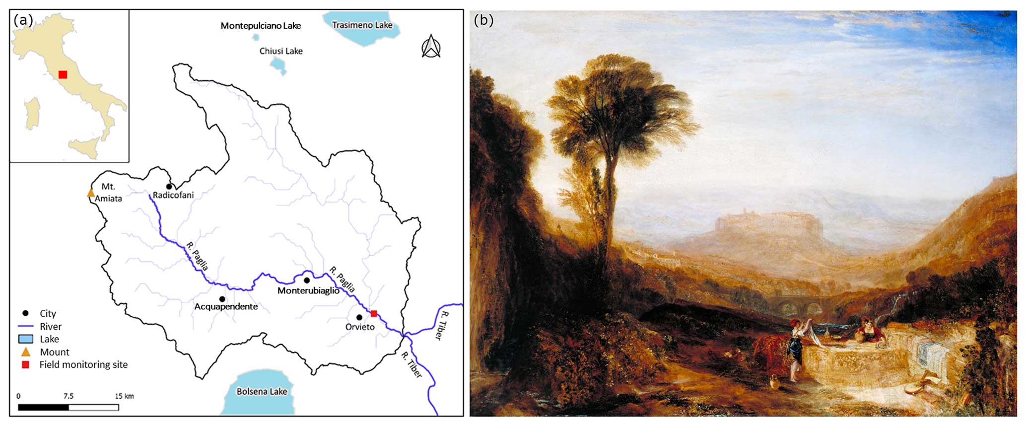
Figure 1Panel (a) presents a map of the Paglia River and its catchment, showing the location of the field monitoring site and of Lake Montepulciano, where the FMs were collected. Panel (b) shows View of Orvieto, Painted in Rome (1828, reworked 1830) by Joseph Mallord William Turner (1775–1851; © photo: Tate, CC BY-NC-ND 3.0, https://www.tate.org.uk/art/artworks/turner-view-of-orvieto-painted-in-rome-n00511, last access: 15 April 2024).
A preliminary survey of the river revealed that the native species of the area, Unio mancus (Lamarck, 1815), is locally extirpated. Therefore, specimens of the same species were collected from the neighbouring Lake Montepulciano (Fig. 1), Siena Province, Tuscany, Italy, on 29 March 2022, and they were maintained in a tank filled with lake water. The mussels were divided into two groups: one group was installed at the field monitoring site in the afternoon of 30 March 2022, whereas the other group was sent to the Hydraulics Laboratory of the University of Trento (Italy) for the flume experiments. On arrival at the laboratory, the animals were acclimated for 2 weeks in a 500 L recirculating flow-through aquarium with aerated water and a gravel–sand substrate, and they were fed with a mixed culture of natural algae. Details of the laboratory and field installation are given in Sect. 2.2.
2.2 Laboratory experiments and in situ installation
The in situ testing of FMs as a possible BEWS for flood events poses a number of challenges, ranging from the selection of the field monitoring site to the choice of the most suitable system for FM installation. The exposure of the animals to the parameters to be monitored is one of the main operational challenges in natural environments. While it is possible to install the animals in lateral derivations of the watercourse or water pipes for the monitoring of chemical contamination, it is essential to expose them to the main channel of the watercourse to monitor their responses to hydrological stresses (i.e. water velocity, turbulence, and sediment transport). This requires installing the FMs in structures that are as transparent as possible to the flow, to ensure that they do not substantially affect the natural flow pattern, and sufficiently stable, to guarantee the integrity of both the FMs and the installation throughout the exposure (e.g. Kramer and Foekema, 2001; Sow et al., 2011). For the sake of logistical convenience, FMs are commonly fixed to solid structures such as steel rods, thereby limiting their ability to move. Furthermore, it is important to note that FMs are frequently used in environmental conditions that may differ from their natural habitat, such as using FMs accustomed to lentic waters in river environments (e.g. Martel et al., 2003), as is the case in the present study.
To assess the extent to which limiting FMs' movement affects their behavioural response to environmental stress, a laboratory experimental comparison was carried out, analysing and comparing valve movements in both freely moving and immobilised animals on vertical rods. These experiments were conducted at the Hydraulics Laboratory of the University of Trento (Italy). The FMs were exposed to the same external conditions for 24 h (Fig. 2). FMs 1 to 4 were free to move, whereas the others, i.e. FMs 5 to 8, were immobilised on vertical rods by gluing one valve to the rod, which was hung vertically from the top of a 10 m long and 40 cm wide flume (Fig. 2b). Free and immobilised FMs were positioned in the middle of the flume, sufficiently far from the upward and downward boundary conditions. After 10 h of continuous discharge at a constant rate of 5.3 L s−1 with 10 cm substratum (and without sediment transport), the discharge was instantaneously increased to 22 L s−1, maintained at this high value for 2 h, and then returned to the initial baseline value (5.3 L s−1). This baseline discharge remained constant during the rest of the experiment, i.e. for the following 12 h. Additional information that we sought during the experiments relates to sediment transport under different discharge configurations, as previous research has shown that FMs are particularly affected by the presence of sediment transport (Modesto et al., 2023; Termini et al., 2023). As reported in Modesto et al. (2023), who conducted experiments using the same flume and discharge settings as those employed in our study, the baseline discharge of 5.3 L s−1 is characterised by negligible sediment transport, whereas the higher discharge of 22 L s−1 involves both bedload and suspended sediment transport. In the same previous study, the critical discharge, i.e. the value corresponding to the onset of sediment transport (also referred to as the incipient condition), was found to be around 14 L s−1. Specifically, this is the discharge value capable of entraining the finest grains (∼0.06 mm in this case) from the mobile bed mixture into the flow.
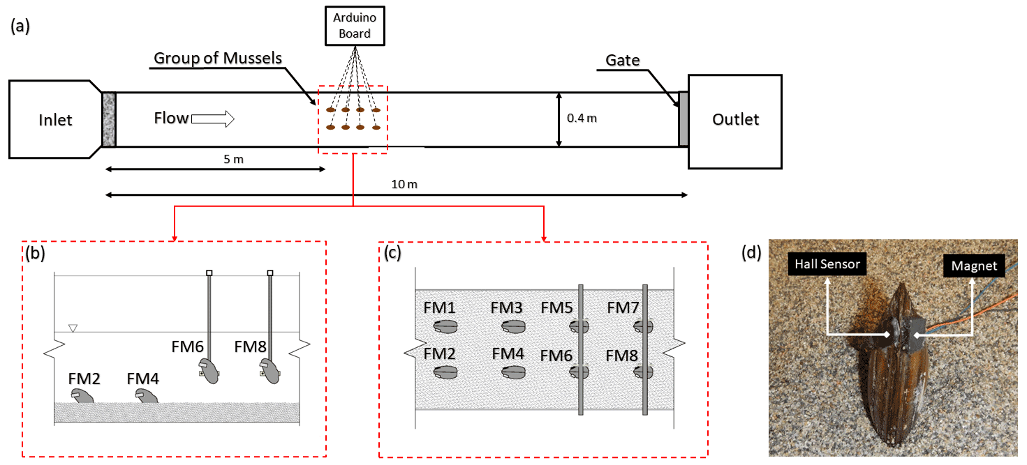
Figure 2Panel (a) outlines the experimental set-up in the laboratory, panels (b) and (c) show the respective side and plan views of the FMs' arrangement in the flume, and panel (d) provides an example of an FM equipped with a Hall sensor and a magnet.
At the Paglia River field monitoring site, 13 FMs were fixed to vertical rods of the same type as those tested in the laboratory and installed in a cage secured at the riverbank. The use of steel rods was deemed necessary to mitigate the risk of FMs being displaced during flood events and due to the unsuitable bedrock substrate at the installation site. The cage was necessary to prevent damage to FMs and electronics. The cage has been designed to ensure robustness while minimising interaction with the flow. To achieve this, a thin steel frame covered by a coarse metal grid was used. The electronics for the valvometry recordings (see Sect. 2.3) were installed on the bridge above the riverbank where the cage was positioned. An overview of the installation is provided in Fig. 3. A multiparameter probe (OTT PLS-C) was installed at the FM cage site to measure the water level, temperature, and conductivity every 10 min. The FMs and multiparameter probe were in place during a flood on 31 March 2022, which is the event analysed in this study.
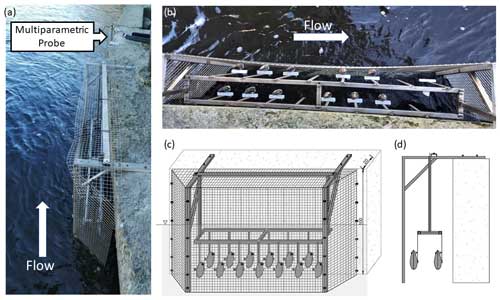
Figure 3Field installation at the ENTERPRISING pilot site, Orvieto, Italy: (a) overview of the FM cage, location of the multiparameter probe, and flow direction; (b) top view of the FM cage; (c) front view (schematic) of the FM cage; and (d) side view (schematic) of the FM cage.
2.3 Valvometry data collection
In order to monitor the frequency and intensity of FM gaping, different valvometry methods have been proposed for over 1 century (reviewed in Vereycken and Aldridge, 2023). In his pioneering work, Marceau (1909) first used a kymograph (i.e. a rotating drum or moving paper strip onto which data are drawn as a function of time) to track the valve movement of mussels by attaching a balanced arm equipped with a scribe to one valve of the mussel. Electromagnetic induction to measure valve displacement was first used by Schuring and Geense (1972) and then further developed thanks to technological advancements. Wilson et al. (2002) introduced the use of the Hall effect to record the valve movement of mussels. This approach requires the installation of a magnet on one valve and a Hall effect sensor on the other valve. The Hall effect sensor measures the magnetic field between the magnet and the sensor itself, which changes according to the distance between the two valves. In this way, both the frequency and intensity of valve gaping can be measured: when the mussel is closed, the magnetic field around the sensor is at its maximum; when the mussel is fully opened, the magnetic field strength around the sensor decreases due to the increased distance between the magnet and the sensor.
In this study, a Hall sensor (Honeywell SS495A1, 13 mm × 10.5 mm, 1.1 g weight) was glued to one side of the mussels' shell and a magnet (12 mm × 10 mm, 1.8 g weight) was glued to the opposite side of the shell (see Fig. 2d). An Arduino board (Mega 2560) was used to record the response of the Hall effect sensor in millivolts (mV), and then, by knowing the minimum and maximum values, the output was normalised and turned to opening percentage (see Sect. 2.4). An SD card connected to the Arduino was used to store the voltage values. In laboratory experiments, each mussel provided data at a frequency of 1 Hz, whereas in the field, due to a different set-up of the recording system, a frequency of 2 Hz was used.
2.4 Signal processing
Due to inherent physiological variations among FMs, primarily influenced by their size and shape, as well as the nonuniform attachment of magnets and sensors to the individuals, describing FM behaviour in terms of the frequency and intensity of gaping using raw data expressed in millivolts may not be straightforward. For this reason, in order to have a common frame of response among all mussels, the opening signals were normalised between 0 % and 100 %, employing linear scaling based on the minimum and maximum values recorded for each FM. Accordingly, 0 % indicates that the mussel's valves are fully closed, whereas 100 % indicates that the mussel's valves are fully open. Before normalising the signal, possible outliers due to occasional acquisition artefacts have been removed. In this context, outliers have been defined using the 0.1 and 99.9 percentiles as the lower- and upper-threshold bounds, respectively. The removed points were subsequently reconstructed through interpolation. It should be noted that, in order to effectively normalise a signal, the signal duration must be long enough to include both the fully closed and fully open periods of the FM.
The resulting FM signals were analysed with the aim of identifying the occurrence of change points in the FMs' behaviour. As discussed in Sect. 1, these changes may be linked to the normal behaviour of non-stressed FMs as well as to the response of these organisms to external perturbations. The monitoring of a sufficiently large number of FMs allowed us to discriminate between the specific behaviour of individual FMs, driven by their own activity, and a systematic response of the FM community to external disturbances. Abrupt change points in the mean of the opening signals were identified using the findchangepts MATLAB function, which is an iterative procedure that detects significant transitions in time-series data through adaptive segmentation of the original time series.
Parallel to abrupt changes in behaviour characterised by steplike discontinuities in the opening signal, it has been observed that FMs exhibit marked changes in both the frequency and intensity of their gaping when they are subject to stress (Modesto et al., 2023; Termini et al., 2023). Here, the statistical analysis of the FM gaping frequencies was carried out using continuous wavelet transform (CWT) analysis, a mathematical technique that decomposes a signal into different frequency components. CWT is particularly useful when dealing with nonstationary signals. Indeed, unlike traditional Fourier analysis, CWT can capture both high- and low-frequency variations in time-series data, making it especially effective for analysing signals that exhibit dynamic changes in frequency and amplitude over time (Meyers et al., 1993; Rhif et al., 2019).
The CWT analysis is based on the convolution of a signal f(t) with a set of functions ψab(t), known as wavelets, derived from translations and dilations of a so-called mother wavelet ψ(t) :
where a is known as the scale factor and b defines a shift in time. Different mother wavelets can be used to decompose a signal, all of which must meet specific conditions (see e.g. Meyers et al., 1993). The convolution of the signal f(t) with the set of wavelets is the wavelet transform:
where the superscript * denotes the complex conjugate and Tψ(a,b) is the wavelet coefficient (which, for the sake of completeness, depends not only on a and b but also on the choice of the mother wavelet ψ). In this way, the signal f(t) is analysed by comparing it to a set of wavelet functions ψab characterised by continuously varying scale a and shift b. Unlike sinusoidal functions in Fourier analysis, these wavelet functions do not have a fixed frequency; rather, they are versatile mathematical functions inherently flexible in both time and frequency domains, which adapt to the nonstationary characteristics of the signal being analysed. The scale factor a is inversely related to frequencies: smaller scales correspond to more “compressed” wavelets (thus higher pseudo-frequencies) and capture details in the signal at shorter timescales, whereas larger scales correspond to more “stretched” wavelets (thus lower pseudo-frequencies) and capture broader features at longer timescales. Note that the term pseudo-frequencies is often used to emphasise that these values should not be confused with the fixed frequencies associated with sinusoidal waves.
The results of the CWT analysis can be effectively visualised through the use of scalograms and pseudo-frequency-averaged (or scale-averaged) wavelet spectra. The scalogram is a graphical representation of signal power distribution across various pseudo-frequencies and through time. It is constructed by considering the absolute value (or magnitude) of the complex wavelet coefficients introduced in Eq. (2) and allows for a comprehensive examination of how different pseudo-frequencies and times contribute to the overall power of the signal. The pseudo-frequency-averaged wavelet spectrum provides a summary of the signal's energy distribution across multiple scales over time, offering insights into both localised and broad-frequency features present in the signal over time. The pseudo-frequency-averaged wavelet spectrum is obtained by scale-averaging the magnitude-squared scalogram over all scales.
In this study, the CWT was computed by applying the cwt function in MATLAB using the Morse wavelet as the mother wavelet to the time series signal of each FM, after removal of abrupt changes in the mean of the opening signal. Identifying and removing step changes in the mean of the signal was necessary to avoid introducing spurious results. In fact, when a CWT decomposition is performed on a signal with an abrupt step change, the result is a mixture of high-frequency components that capture the abrupt transition and lower-frequency components that describe the smoother and more gradual changes in the signal, across the entire frequency spectrum. The presence of abrupt changes would generate an artefact in the resulting scalograms and pseudo-frequency-averaged wavelet spectra, possibly hindering the interpretation of the informative features of the signal. Step change removal was achieved by detrending the segments of the signal between two successive step changes (identified as discussed above), i.e. by subtracting the mean and removing the linear trend, hence without altering the informative, high-frequency content of the original signal.
Similar to the signal preprocessing described above, in order to get a consistent frame of reference, the scalogram of each FM was normalised between the minimum and maximum values after the removal of outliers. This allows us to effectively appreciate the existence of coherent features across FMs and characterise them in terms of dominant pseudo-frequencies and position in time. In order to obtain a synthetic summary of the results, the normalised scalograms obtained from the wavelet analysis of all FMs were combined into one, corresponding to the median scalogram. The summary pseudo-frequency-averaged wavelet spectra was obtained from the median scalogram.
3.1 Laboratory results
The median opening signal of the FMs measured during the 24 h laboratory experiment along with the 25th and 75th percentiles are shown in Fig. 4a for free and immobilised mussels, respectively. The evolution of discharge in time is also shown in the second y axis. The figure clearly shows that both groups of FMs responded to the discharge increase, 10 h after the start of the experiment, with a sharp and localised change in the median opening (thick coloured lines). By examining the shaded area of this plot (representing the 25th and 75th percentiles), it becomes evident that the signals from free FMs generally exhibit a more complex and varied behaviour compared with those of immobilised FMs. Indeed, if we analyse the periods away from the discharge perturbation, the shaded area for the free FMs is much thicker than that of immobilised FMs. This is explained by the fact that the former group displayed a larger number of features, most of which did not appear to be directly related to hydrodynamic changes. For instance, a decrease in the median opening of free FMs 6 h after the start of the experiment is apparent and is not related to a consistent response across the four free FMs, rather to independent and uncorrelated activities of the organisms. This is further evidenced in Fig. S1 in the Supplement, which illustrates the distinct behavioural patterns exhibited by each FM and the major discontinuities in the mean of the signal. However, during the perturbation (from 10 to 12 h after the start of the experiment), the width of the shaded area (25th–75th percentiles) shrinks and matches that of the immobilised FMs, indicating a coherent response across the four free FMs.
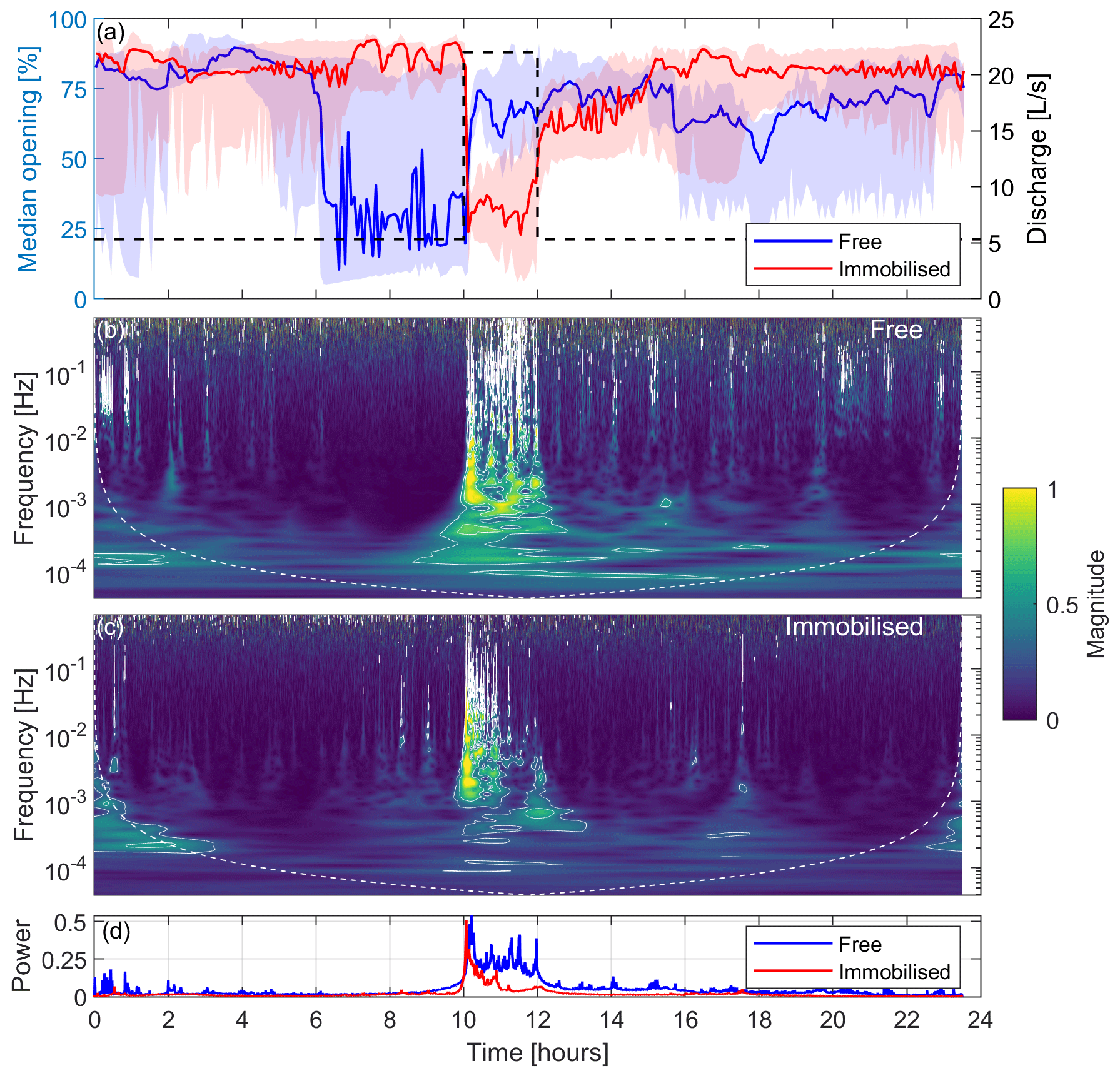
Figure 4Laboratory experiment: the left y axis in panel (a) shows the median valve-opening signals of free and immobilised mussels, with the 25th and 75th percentiles indicated by the shaded area, whereas the right y axis in panel (a) presents discharge (dashed black line); panel (b) is a scalogram showing the median normalised magnitude of the continuous wavelet transform over all of the free FMs; panel (c) is a scalogram showing the median normalised magnitude of the continuous wavelet transform over all the immobilised FMs; and panel (d) presents a pseudo-frequency-averaged wavelet spectrum. White contours in panels (b) and (c) represent the 95th and 99th percentiles of the CWT coefficient.
The distinction between the two groups of mussels arises from the restricted mobility of immobilised FMs in contrast with free FMs, as behaviours such as walking and drifting are not possible, resulting in a more straightforward signal. Notably, all immobilised FMs responded by closing their valves when the discharge increased, whereas two out of the four free FMs responded with an increase in the opening (FM1 and FM2) and one responded with a decrease (FM4; see Fig. S1). Apart from exhibiting some noise, likely arising from electrical issues, which did not significantly impact the results, free FM3 displayed a behaviour similar to that of FM4. While both free and immobilised FMs responded clearly and promptly to the rapid increase in discharge, as evidenced by the change in the mean valve opening discussed above, only immobilised mussels displayed a similar response upon the re-establishment of the base flow (12 h after the start of the experiment), albeit to a lesser extent compared with the signal variation the mussels exhibited when the flow increased (Figs. 4a and S1).
Moving beyond the analysis of mean valve opening, however, a distinct signature of the discharge perturbation is discernible in both free and immobilised FMs through the occurrence of broad-frequency features localised over time around the perturbation period (see the period between 10 and 12 h in Figs. S1 and S2, with the latter showing the signals after detrending and removal of changes in the mean valve opening). Such features are more clearly appreciable when looking at the scalograms of free (Fig. 4b) and immobilised (Fig. 4c) FMs. Prior to the increase in discharge (from the beginning of the experiment to 10 h), the FMs' gaping was characterised by low pseudo-frequencies (below 10−3 Hz) with less energy. However, following the increase in discharge, they promptly began responding across the whole range of pseudo-frequencies (up to 1 Hz), displaying higher energy levels (as indicated by the more yellowish regions). The white contours on the scalogram plot represent the 95th and 99th percentiles of the CWT coefficient and were used to emphasise the energy-rich areas. The response is similar between free and immobilised FMs, although immobilised FMs adapted quicker to the new discharge conditions compared with free FMs. This is evident also looking at Fig. 4d, which shows the pseudo-frequency-averaged wavelet spectrum for both FM classes: immobilised mussels' power returned to normal 1 h after the discharge increase, whereas free mussels responded with high power until the end of the event (2 h after the discharge increase). In both cases, the dominant pseudo-frequencies, after the discharge variations, reset to values consistent with those characterising the first part of the experiment.
3.2 Field results
Because laboratory experiments showed overall consistent responsiveness between free and immobilised FMs in the presence of hydrodynamic stresses, this supported the suitability of installing immobilised FMs in the field. Figure 5a illustrates the signals of the 13 immobilised FMs at the field monitoring site along the Paglia River (see Figs. 1 and 3) from 22:00 LT (local time, UTC+2) on 30 March 2022 until 00:00 LT (midnight) on 1 April 2022. It should be mentioned that there is a gap of 1.5 h in the data for all FMs, with missing signals from mussels between 10.5 and 12 h from the start of the signal (i.e. between 08:30 and 10:00 LT on 31 March) due to unspecified technical issues. According to Fig. 5a, all FMs except for FM2, FM3, and FM12 experienced a marked shift in the mean valve opening with a generalised closing of the valves approximately 5.5 h after the start of the time series, specifically around 03:30 LT on 31 March, coinciding with a flood event in the river. As can be observed in the data, the sensor installed on FM2 experienced technical issues, preventing its use in the analysis. On the other hand, the sensors installed on FM3 and FM12 were operating normally, but the FMs had already closed before the flood event (likely because they were in a resting state; see Sect. 1); hence, FM3 and FM12 did not displaying any additional closure, rather a minor and progressive opening and gaping. All of the other 10 FMs were characterised by normal behaviour before the flood event, with their valves open, and displayed regular valve movements as expected during respiration and filtration.
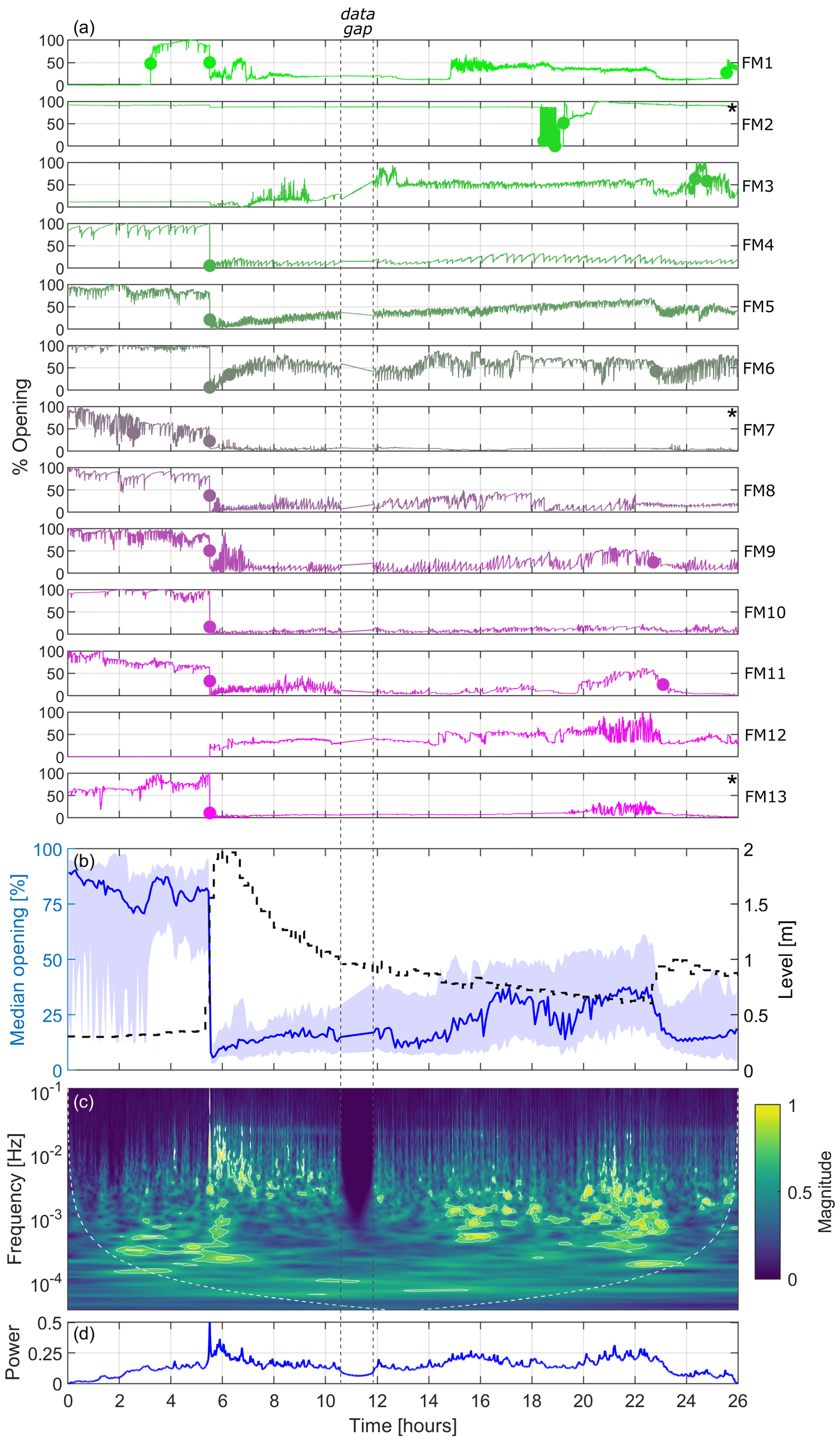
Figure 5Results from the 13 FMs deployed at the Paglia River field monitoring site during the flood on 31 March 2022: panel (a) shows the valve-opening signals for the individual FMs (dots indicate abrupt change points in the mean of the opening signals when the mean opening changes by more than 25 %, while the asterisk (*) depicts FMs that are excluded from the wavelet transform analysis); in panel (b), the left y axis shows the median valve-opening signals, with 25th and 75th percentiles indicated by the shaded area (all FMs except FM2), while the right y axis presents the water level (dashed black line); panel (c) is a scalogram showing the median normalised magnitude of the continuous wavelet transform over the FMs; and panel (d) shows a pseudo-frequency-averaged wavelet spectrum. White contours in panel (c) represent the 95th and 99th percentiles of the CWT coefficient.
In general, in terms of change in the mean valve opening, the mussels responded similarly to changes in hydrodynamic conditions, as observed in the flume experiment and illustrated in Fig. 5b, which depicts the median valve-opening signal of the FMs (all individuals except FM2) in relation to the changes in water level measured by the multiparameter sensor every 10 min (see also Fig. S3). The median valve opening shows two main discontinuities that coincide with marked changes in the water level line. The first discontinuity is evident at 5.5 h from the start of the time series (i.e. at 03:30 LT), when the water level, as measured by the multiparameter sensor, rapidly increased from 0.3 m (corresponding to about 4 m3 s−1) to 2 m (corresponding to about 140 m3 s−1), based on the data from the official gauging station, available every 30 min. This rise in water level marked the onset of the flood event, which was characterised by a sharply rising front. The associated discontinuity in the valve-opening signal is clearly visible when examining both the individual FM signals (Fig. 5a) and the median signal (Fig. 5b). The second discontinuity clearly emerges only by looking at the median signal (Fig. 5b), while it is hindered in the individual time series. It occurred at about 23 h after the start of the time series (i.e. at 21:00 LT), when the water level rose from 0.6 m (approximately 18 m3 s−1) to 1 m (approximately 45 m3 s−1), thus interrupting the previously gradual decrease in the water level following the initial peak.
The FMs response to the hydrodynamic disturbance, as reflected in changes in the frequency of gaping, is shown in the scalogram of Fig. 5c. This plot is obtained by excluding FM2, which was affected by the technical issues discussed above, and (for the sake of clarity) FM7 and FM13, which were characterised by intense activity before the flood and a significantly damped response after the flood, respectively, to an extent that was not in alignment with the behaviour of the other FMs. These mussels are labelled with * in Fig. 5a (and in the corresponding Fig. S4 showing the signals after detrending and removal of changes in the mean valve opening). As indicated by the scalogram, the mussels exhibited responses at a low frequency (below 10−4–10−3 Hz) before the peak of the flood, displaying signals of lower energy. As soon as the level increased, parallel to the sudden closure of the valves seen in Fig. 5a and b, the FMs showed a generalised response shifted towards higher frequencies (up to 0.1 Hz) and characterised by higher energy levels (yellowish regions). This response gradually diminished as the discharge decreased, resulting in lower frequencies and reduced energy levels. Between 15 and 23 h from the beginning of the time series, the water level, and consequently the discharge, transitioned into the latter phase of the flood event, characterised by minor fluctuations over time. Additionally, water temperature and conductivity steadily returned to higher values and stabilised (see Fig. S3). During this time window, the FMs underwent a slight opening of the valves (Fig. 5b) and intensified their gaping around frequencies of 10−3 Hz (Fig. 5c). Following the occurrence of the second, smaller peak in water level (approximately 23 h after the start of the time series), all FMs closed their valve once more (Fig. 5b) and the majority of them exhibited a significant decrease in the frequency of gaping (Fig. 5a and c). The overall picture is also summarised in the pseudo-frequency-averaged wavelet spectrum shown in Fig. 5d, which clearly indicates the instantaneous evident response of the FMs to the main perturbation, similar to what was observed in the laboratory experiments.
In recent research based on laboratory experiments, Modesto et al. (2023) and Termini et al. (2023) proposed FMs as effective BEWSs to assess the impact of hydrodynamic stresses on the aquatic ecosystem. In this study, for the first time, FMs were deployed and evaluated under real river conditions, in the Paglia River at Orvieto, Italy. The initial challenge that we faced was securing the mussels in place and preventing them from being carried away by the river's current. In consideration of other in situ exposure methods (e.g. Kramer and Foekema, 2001; Sow et al., 2011), we opted to glue the mussels to vertical rods anchored at the riverbank. To ensure that the use of immobilised mussels did not significantly alter their behavioural responsiveness, we conducted controlled laboratory experiments to confirm that immobilised and free mussels exhibit consistent reactions to the same hydrodynamic stressors.
The results demonstrated that immobilised and free mussels behave in a consistent way during a hydrodynamic perturbation, but the signals of the immobilised mussels exhibit less complexity, primarily due to the reduced number of features resulting from movement constraints (Fig. 4). Consequently, these signals can be more easily interpreted and associated with perturbations in external conditions. In fact, immobilised mussels have limited means of response, primarily relying on gaping, as they are unable to engage in actions such as escaping or burying themselves more deeply. It is worth noting that, concerning mussel behaviour classification, both free and immobilised mussels showed avoidance behaviour by immediately closing their valves and changing their gaping frequency at the onset of the higher flow levels. However, immobilised mussels showed a faster adaptation in response to a prolonged stimulus, facilitating the faster restoration of pre-event gaping frequencies. This could be explained by the positive correlation between the intensity of the stimulus and the degree of adaptation (Hollins et al., 1990). In fact, immobilised mussels experience a stronger stimulus than free mussels due to the impossibility of actively searching for shelter at the time of the event; as a result, they have a shorter adaptation period, most likely because they get tired sooner. Overall, based on the laboratory comparison, we could confidently assert that the installation of immobilised mussels under real river conditions ensures both site stability during floods and the representativeness of the results. This is particularly true in the context of using FMs as real-time BEWSs, which requires timely detection of significant changes, while other information such as response type and duration may be of interest for deeper biological interpretation but is not the primary concern.
Field data acquired at the field monitoring site in the Paglia River provided a solid validation of the effectiveness and reliability of using immobilised mussels as part of a real-time BEWS. All of the FMs exhibited a synchronised and highly distinct response to the flood event that occurred during the monitoring campaign, promptly transitioning their behaviour in terms of both mean valve-opening and valve-gaping frequency. Of paramount importance for practical applications is the observation that these mussels responded immediately as the discharge increased, effectively detecting the flood at its very onset. These results confirm and validate what has been observed in the laboratory: sharp and rapid mussel reactions can be explained by the almost abrupt rise in water levels and discharges of the flood as well as by the fact that, as in the flume experiments (see Sect. 2.2), the discharge values around the peak triggered sediment transport and turbidity. To establish an incipient (alias critical) discharge value for the Paglia River, we exploited the shear stress distribution relative to the flood on 31 May 2022, determined by a 3D Reynolds-averaged Navier–Stokes (3D-RANS) model described in Bahmanpouri et al. (2023), and some bed material samples that we collected from the bed surface just upstream and downstream of the Adunata Bridge site. With a constant flow discharge corresponding to that observed at the flood peak, the numeric shear stress distribution reached a maximum of about 100 Pa under the bridge, whereas smaller values were observed away from the bridge. Looking at the numerical results, a reference value of 30 Pa is exerted over a large part of the flow domain. From the bed material sample, we found that the d90 (i.e. diameter corresponding to the 90th percentile of the granulometric distribution) of the sediments forming the substrate of the bed is about 0.01 m. With these values, the well-known dimensionless Shields stress number , where τ is the bottom shear stress, ρs(ρw) is the sediment (water) density, g the gravitational constant, and d the characteristic particle diameter, reached a value of about 0.6 at the discharge peak, well above the critical value, which can be assumed to be equal to about 0.06, as in many references (see e.g. Pähtz and Durán, 2018). According to the 3D-RANS model, a critical discharge for the initiation of bedload in this reach of Paglia River (Adunata Bridge) corresponds to about 4 m3 s−1. Therefore, the ratio, in terms of peak flood discharge over the critical value, is about 35 (i.e. ), whereas the mussels experienced a discharge about 1.6 times larger than the critical value (i.e. ) in the flume experiments, in accordance with the data reported in Sect. 2.2. Our laboratory and field results show that the responsiveness of the mussels is efficient over a wide range of peak-to-critical-discharge ratios.
To improve the interpretation of behavioural signals, we proposed a statistical analysis based on the combined identification of abrupt change points in the mean of the opening signals and the application of continuous wavelet transform to the detrended time series after removal of these discontinuities (refer to Figs. S2 and S4 to view the cleaned signals). This approach has proven to be a robust and reliable tool for FM signal processing and is able to effectively identify the animals' response to external stressors. This identification can be achieved both visually, through the examination of scalogram plots, and quantitatively, through the generation of associated pseudo-frequency-averaged wavelet spectrum plots. For the sake of comparability, the scalogram of each FM was normalised between the minimum and maximum values after the removal of outliers. Then, the median scalogram was calculated and used to identify dominant pseudo-frequencies and their temporal positions. This approach enables comparisons within the same frame of reference between different FMs and between median scalograms obtained under various conditions (e.g. in the laboratory and in the river). Similarly, the pseudo-frequency-averaged wavelet spectra derived from the median scalograms can be fairly compared to discern shared patterns and distinctions across the various set-ups. Notably, results from both the laboratory and the field indicate that the power of the spectrum reached and exceeded a value of approximately 0.25 during external stress events (i.e. an increase in discharge). While further data collection from additional sites is needed before proposing a threshold value as a simple indicator of aquatic ecosystem stress, these findings underscore the effectiveness of combining FM valvometry and CWT processing towards the establishment of real-time operational BEWSs.
The utilisation of FMs under real riverine conditions did present logistical challenges. While the monitoring station at the Paglia River was operational for several months, the data acquired only covered the occurrence of a flood. The lack of significant events during the monitoring period and the mortality of some FMs prevented the acquisition of additional data that would have been valuable for the analysis. Additionally, during the monitoring activity after the flood event occurred on 30 March 2022, metal particles that were occasionally suspended in the water, likely originating from an upstream mine, accumulated on the magnets installed on the FMs, thereby altering the valvometric signal. In addition, the extrapolation of laboratory results to natural conditions should consider the greater variability in boundary conditions with respect to the parameter being monitored. The response of the mussels is an expression of their reaction to changes in multiple conditions that can only be controlled and restored to previous conditions in the laboratory (and even then not completely). In this respect, the increased activity in terms of energy content at the highest frequencies observed at the end of the descending phase of the flood in the Paglia River (see Fig. 5c and d, between 20 and 23 h) cannot be explained based on the available measurements. For example, the water temperature (see Fig. S3) should not be influential, as it was always below the tolerance threshold of the eurythermal generalist species that we used and showed minor changes during the period analysed (about 1.5 °C). It is likely that other environmental variables, such as turbidity or specific FM behaviour after a long disturbance, were involved. For these reasons, efforts to expand the dataset for a more comprehensive analysis are planned and underway, and further studies should be conducted to deepen the behavioural characteristics of the FMs in the field, investigate the limitations of the method, and develop protocols to address them appropriately.
The results obtained pave the way for the utilisation of the valvometry technique and of the signal-processing framework presented here in operational BEWSs in different contexts. Freshwater mussels can serve as indicators to quantify the impact of both natural stressors (e.g. heat waves and droughts) and anthropogenic stressors (e.g. hydropeaking, reservoir flushing, and chemical contamination) on the aquatic ecosystem. As such, they can be instrumental in reporting the impacts of climate change on water resources and in the management and permit processes implemented by local authorities. Future research should focus on extending the investigation of the responsiveness of FMs to other stressors (e.g. turbidity, temperature, and chemicals) and on verifying the effectiveness of the signal-processing technique presented here in identifying possible synthetic indicators related to different stressors.
In summary, based on the above insights, the following conclusions can be drawn:
-
Both free and immobilised freshwater mussels can serve as effective ecosystem warning indicators in aquatic environments, with the choice between them depending on the riverbed and flow rate conditions.
-
Immobilising the mussels to support constrains their behaviour, but this results in sharper event detection (compared with free mussels) and easier interpretation of the signals.
-
Continuous wavelet transform proves to be a valuable tool for interpreting FM signals. It is effective in identifying pseudo-frequency features present in the signal over time and describing the response of FMs to external perturbations, providing more informative results than only looking at discontinuities in the opening time series.
-
Laboratory and field experiments with immobilised mussels demonstrate their response to hydrodynamic stresses within a frequency of valve gaping ranging from 10−3 to 1 Hz. This frequency range is larger than the background frequency range during normal behaviour (around 10−4–10−3 Hz when taking the median across multiple individuals). These frequency values correspond to conditions that indicate the presence of stressful conditions for FMs, thus underscoring the potential use of FMs as real-time BEWSs to identify potential threats to the aquatic ecosystem.
-
The comparison between pseudo-frequency-averaged wavelet spectra obtained in the laboratory and those obtained in the field suggests the potential introduction (subject to further data acquisition) of a simple indicator based on power values to detect disturbances in the aquatic environment.
The data and code that support the study are available from the corresponding author upon request.
The supplement related to this article is available online at: https://doi.org/10.5194/hess-28-2297-2024-supplement.
AP: investigation, methodology, formal analysis, data curation, and writing – original draft. NR: conceptualisation, investigation, methodology, resources, supervision, and writing – original draft. NB: investigation and writing – review and editing. VM: investigation, resources, and writing – review and editing. DT: funding acquisition, conceptualisation, investigation, and writing – review and editing. DM, AB, and CC: data curation. TL: data curation and writing – review and editing. TM: funding acquisition, project administration, conceptualisation, investigation, and writing – review and editing. LF: conceptualisation, investigation, methodology, supervision, funding acquisition, and writing – review and editing. SP: conceptualisation, investigation, methodology, software, formal analysis, data curation, visualisation, supervision, and writing – original draft.
The contact author has declared that none of the authors has any competing interests.
Publisher’s note: Copernicus Publications remains neutral with regard to jurisdictional claims made in the text, published maps, institutional affiliations, or any other geographical representation in this paper. While Copernicus Publications makes every effort to include appropriate place names, the final responsibility lies with the authors.
We thank the anonymous reviewers for their constructive comments.
This research has been supported by the Ministero dell'Istruzione, dell'Università e della Ricerca (grant no. 2017SEB7Z8).
This paper was edited by Thom Bogaard and reviewed by two anonymous referees.
Akberali, H. B. and Davenport, J.: The detection of salinity changes by the marine bivalve molluscs Scrobicularia plana (da Costa) and Mytilus edulis L., J. Exp. Mar. Biol. Ecol., 58, 59–71, 1982. a
Antala, M., Juszczak, R., van der Tol, C., and Rastogi, A.: Impact of climate change-induced alterations in peatland vegetation phenology and composition on carbon balance, Sci. Total Environ., 827, 154294, https://doi.org/10.1016/j.scitotenv.2022.154294, 2022. a
Bae, M.-J. and Park, Y.-S.: Biological early warning system based on the responses of aquatic organisms to disturbances: a review, Sci. Total Environ., 466, 635–649, 2014. a
Bahmanpouri, F., Lazzarin, T., Barbetta, S., Moramarco, T., and Viero, D. P.: Estimating flood discharge at river bridges using the entropy theory. Insights from Computational Fluid Dynamics flow fields, Hydrol. Earth Syst. Sci. Discuss. [preprint], https://doi.org/10.5194/hess-2023-253, in review, 2023. a
Barron, O., Silberstein, R., Ali, R., Donohue, R., McFarlane, D. J., Davies, P., Hodgson, G., Smart, N., and Donn, M.: Climate change effects on water-dependent ecosystems in south-western Australia, J. Hydrol., 434, 95–109, 2012. a
Beggel, S. and Geist, J.: Acute effects of salinity exposure on glochidia viability and host infection of the freshwater mussel Anodonta anatina (Linnaeus, 1758), Sci. Total Environ., 502, 659–665, 2015. a
Borcherding, J.: Valve movement of the mussel Dreissena polymorpha as a monitoring system for bodies of water, Schriftenreihe des Vereins für Wasser-, Boden-und Lufthygiene, 89, 361–373, 1992. a
Butterworth, F. M., Villalobos-Pietrini, R., and Gonsebatt, M. E.: Introduction: Biomonitors and Biomarkers as Indicators of Environmental Change, Volume 2, in: Biomonitors and Biomarkers as Indicators of Environmental Change 2: A Handbook, 1–8, Springer, ISBN 0306463873, 2001. a
Cairns, J.: Biological monitoring – concept and scope, in: Environmental biomonitoring, assessment, prediction and management, edited by: Cairns, J., Patil, G. P., and Waters, W. E., Int. Co-op Publ. House, ISBN 0899740081, 1979. a
Cao, Q., Yu, G., Sun, S., Dou, Y., Li, H., and Qiao, Z.: Monitoring water quality of the Haihe River based on ground-based hyperspectral remote sensing, Water, 14, 22, https://doi.org/10.3390/w14010022, 2022. a
Chowdury, M. S. U., Emran, T. B., Ghosh, S., Pathak, A., Alam, M. M., Absar, N., Andersson, K., and Hossain, M. S.: IoT based real-time river water quality monitoring system, Procedia Comput. Sci., 155, 161–168, 2019. a
Davenport, J.: The isolation response of mussels (Mytilus edulis L.) exposed to falling sea-water concentrations, J. Mar. Biol. Assoc. UK, 59, 123–132, 1979. a
Davenport, J.: The opening response of mussels (Mytilus edulis) exposed to rising sea-water concentrations, J. Mar. Biol. Assoc. UK, 61, 667–678, 1981. a
Dvoretsky, A. G. and Dvoretsky, V. G.: Shellfish as biosensors in online monitoring of aquatic ecosystems: A review of Russian studies, Fishes, 8, 102, https://doi.org/10.3390/fishes8020102, 2023. a
Folegot, S., Bruno, M. C., Larsen, S., Kaffas, K., Pisaturo, G. R., Andreoli, A., Comiti, F., and Maurizio, R.: The effects of a sediment flushing on Alpine macroinvertebrate communities, Hydrobiologia, 848, 3921–3941, 2021. a
Gerhardt, A., Ingram, M. K., Kang, I. J., and Ulitzur, S.: In situ on‐line toxicity biomonitoring in water: Recent developments, Environ. Toxicol. Chem., 25, 2263–2271, 2006. a
Gitelson, A., Garbuzov, G., Szilagyi, F., Mittenzwey, K. H., Karnieli, A., and Kaiser, A.: Quantitative remote sensing methods for real-time monitoring of inland waters quality, Int. J. Remote Sens., 14, 1269–1295, 1993. a
Goldberg, E. D.: The mussel watch-a first step in global marine monitoring, Pollution Bulletin, 6, 111–114, https://doi.org/10.1016/0025-326X(75)90271-4, 1975. a
Gruber, D. and Diamond, J: Automated Biomonitoring: Living Sensors as Environmental Monitors, Ellis Horwood books in aquaculture and fisheries support, E. Horwood, ISBN 9780745803104, 1988. a
Gsell, A. S., Scharfenberger, U., Özkundakci, D., Walters, A., Hansson, L.-A., Janssen, A. B. G., Nõges, P., Reid, P. C., Schindler, D. E., and Van Donk, E.: Evaluating early-warning indicators of critical transitions in natural aquatic ecosystems, P. Natl. Acad. Sci. USA, 113, E8089–E8095, 2016. a
Guterres, B. V., Junior, J. N. J., Guerreiro, A. S., Fonseca, V. B., Botelho, S. S. C., and Sandrini, J. Z.: Intelligent classifiers on the construction of pollution biosensors based on bivalves behavior, in: Brazilian Conference on Intelligent Systems, Springer, 588–603, https://doi.org/10.1007/978-3-030-61380-8_40, 2020. a
Hartmann, J. T., Beggel, S., Auerswald, K., Stoeckle, B. C., and Geist, J.: Establishing mussel behavior as a biomarker in ecotoxicology, Aquat. Toxicol., 170, 279–288, 2016. a, b
Hernandez-Ramirez, A. G., Martinez-Tavera, E., Rodriguez-Espinosa, P. F., Mendoza-Pérez, J. A., Tabla-Hernandez, J., Escobedo-Urías, D. C., Jonathan, M. P., and Sujitha, S. B.: Detection, provenance and associated environmental risks of water quality pollutants during anomaly events in River Atoyac, Central Mexico: A real-time monitoring approach, Sci. Total Environ., 669, 1019–1032, 2019. a
Higgins, P. J.: Effects of food availability on the valve movements and feeding behavior of juvenile Crassostrea virginica (Gmelin). I. Valve movements and periodic activity, J. Exp. Mar. Biol. Ecol., 45, 229–244, 1980. a
Hollins, M., Goble, A. K., Whitsel, B. L., and Tommerdahl, M.: Time course and action spectrum of vibrotactile adaptation, Somatosens. Mot. Res., 7, 205–221, 1990. a
Holt, E. A. and Miller, S. W.: Bioindicators: Using organisms to measure, Nature, 3, 8–13, 2011. a
Kramer, K. J. M. and Foekema, E. M.: The “Musselmonitor®” as Biological Early Warning System: The First Decade, Biomonitors and biomarkers as indicators of environmental change 2: a handbook, 59–87, https://doi.org/10.1007/978-1-4615-1305-6_4, 2001. a, b
Kramer, K. J. M., Jenner, H. A., and de Zwart, D.: The valve movement response of mussels: a tool in biological monitoring, Hydrobiologia, 188, 433–443, 1989. a, b, c
Lamarck, J.-B. P. A. d. M.: Histoire naturelle des animaux sans vertèbres ... précédée d'une introduction offrant la détermination des caractères essentiels de l'animal, sa distinction du végétal et des autres corps naturels, enfin, l'exposition des principes fondamentaux de la zoologi, vol. t.1, Paris: published by the author, https://www.biodiversitylibrary.org/item/47694 (last access: 15 April 2024), 1815. a
Lewsey, C., Cid, G., and Kruse, E.: Assessing climate change impacts on coastal infrastructure in the Eastern Caribbean, Mar. Policy, 28, 393–409, 2004. a
Li, L., Zheng, B., and Liu, L.: Biomonitoring and bioindicators used for river ecosystems: definitions, approaches and trends, Procedia Environ. Sci., 2, 1510–1524, 2010. a
Makanda, K., Nzama, S., and Kanyerere, T.: Assessing the role of water resources protection practice for sustainable water resources management: a review, Water, 14, 3153, https://doi.org/10.3390/w14193153, 2022. a
Marceau, F.: Recherches sur la morphologie, l'histologie et la physiologie comparées de muscles adducteurs des mollusques acéphales, Archives de Zoologie Paris, 295–469, https://eurekamag.com/research/023/471/023471788.php (last access: 15 April 2024), 1909. a
Martel, P., Kovacs, T., Voss, R., and Megraw, S.: Evaluation of caged freshwater mussels as an alternative method for environmental effects monitoring (EEM) studies, Environ. Pollut., 124, 471–483, 2003. a
Meng, F., Fu, G., and Butler, D.: Cost-effective river water quality management using integrated real-time control technology, Environ. Sci. Technol., 51, 9876–9886, 2017. a
Metcalfe, R. A., Mackereth, R. W., Grantham, B., Jones, N., Pyrce, R. S., Haxton, T., Luce, J. J., and Stainton, R.: Aquatic ecosystem assessments for rivers, Ministry of Natural Resources, Peterborough, ON, Canada, ISBN 978-1-4606-3215-4, 2013. a
Meyers, S. D., Kelly, B. G., and O'Brien, J. J.: An introduction to wavelet analysis in oceanography and meteorology: With application to the dispersion of Yanai waves, Mon. Weather Rev., 121, 2858–2866, 1993. a, b
Modesto, V., Tosato, L., Pilbala, A., Benistati, N., Fraccarollo, L., Termini, D., Manca, D., Moramarco, T., Sousa, R., and Riccardi, N.: Mussel behaviour as a tool to measure the impact of hydrodynamic stressors, Hydrobiologia, 850, 807–820, 2023. a, b, c, d, e, f
Nagai, K., Honjo, T., Go, J., Yamashita, H., and Oh, S. J.: Detecting the shellfish killer Heterocapsa circularisquama (Dinophyceae) by measuring bivalve valve activity with a Hall element sensor, Aquaculture, 255, 395–401, 2006. a
Nawar, A. K. and Altaleb, M. K.: A low-cost real-time monitoring system for the river level in wasit province, in: 2021 International Conference on Advance of Sustainable Engineering and its Application (ICASEA), IEEE, 54–58, ISBN 166549736X, 2021. a
Pähtz, T. and Durán, O.: The cessation threshold of nonsuspended sediment transport across aeolian and fluvial environments, J. Geophys. Res.-Earth, 123, 1638–1666, 2018. a
Pasika, S. and Gandla, S. T.: Smart water quality monitoring system with cost-effective using IoT, Heliyon, 6, e04096, https://doi.org/10.1016/j.heliyon.2020.e04096, 2020. a
Piccolroaz, S., Toffolon, M., Robinson, C. T., and Siviglia, A.: Exploring and quantifying river thermal response to heatwaves, Water, 10, 1098, https://doi.org/10.3390/w10081098, 2018. a
Qu, S., Wang, L., Lin, A., Yu, D., and Yuan, M.: Distinguishing the impacts of climate change and anthropogenic factors on vegetation dynamics in the Yangtze River Basin, China, Ecol. Indic., 108, 105724, https://doi.org/10.1016/j.ecolind.2019.105724, 2020. a
Rhif, M., Ben Abbes, A., Farah, I. R., Martínez, B., and Sang, Y.: Wavelet transform application for/in non-stationary time-series analysis: A review, Appl. Sci., 9, 1345, https://doi.org/10.3390/app9071345, 2019. a
Robson, A. A., Thomas, G. R., De Leaniz, C. G., and Wilson, R. P.: Valve gape and exhalant pumping in bivalves: optimization of measurement, Aquat. Biol., 6, 191–200, 2009. a
Salánki, J., Farkas, A., Kamardina, T., and Rózsa, K. S.: Molluscs in biological monitoring of water quality, Toxicol. Lett., 140–141, 403–410, https://doi.org/10.1016/S0378-4274(03)00036-5, 2003. a
Scanlon, B. R., Fakhreddine, S., Rateb, A., de Graaf, I., Famiglietti, J., Gleeson, T., Grafton, R. Q., Jobbagy, E., Kebede, S., and Kolusu, S. R.: Global water resources and the role of groundwater in a resilient water future, Nature Reviews Earth & Environment, 4, 87–101, 2023. a
Schöne, B. R. and Krause Jr., R. A.: Retrospective environmental biomonitoring–Mussel Watch expanded, Global Planet. Change, 144, 228–251, 2016. a
Schuring, B. J. and Geense, M. J.: Een electronische schakeling voor het registreren van openingshoek van de mossel Mytilus edulis L, TNO-Rapport CL, 72, 1972. a
Siddig, A. A. H., Ellison, A. M., Ochs, A., Villar-Leeman, C., and Lau, M. K.: How do ecologists select and use indicator species to monitor ecological change? Insights from 14 years of publication in Ecological Indicators, Ecol. Indic., 60, 223–230, 2016. a
Sow, M., Durrieu, G., Briollais, L., Ciret, P., and Massabuau, J.-C.: Water quality assessment by means of HFNI valvometry and high-frequency data modeling, Environ. Monit. Assess., 182, 155–170, 2011. a, b, c, d
Sukanya, S. and Joseph, S.: Climate change impacts on water resources: An overview, in: Visualization Techniques for Climate Change with Machine Learning and Artificial Intelligence, 55–76, https://doi.org/10.1016/B978-0-323-99714-0.00008-X, Elsevier, 2023. a
Swapna, M., Viswanadhula, U. M., Aluvalu, R., Vardharajan, V., and Kotecha, K.: Bio-signals in medical applications and challenges using artificial intelligence, Journal of Sensor and Actuator Networks, 11, 17, https://doi.org/10.3390/jsan11010017, 2022. a
Termini, D., Benistati, N., Tosato, L., Pilbala, A., Modesto, V., Fraccarollo, L., Manca, D., Moramarco, T., and Riccardi, N.: Identification of hydrodynamic changes in rivers by means of freshwater mussels' behavioural response: an experimental investigation, Ecohydrology, e2544, https://doi.org/10.1002/eco.2544, 2023. a, b, c, d, e
Tran, D., Ciret, P., Ciutat, A., Durrieu, G., and Massabuau, J.: Estimation of potential and limits of bivalve closure response to detect contaminants: application to cadmium, Environ. Toxicol. Chem., 22, 914–920, 2003. a
Tran, D., Fournier, E., Durrieu, G., and Massabuau, J.: Inorganic mercury detection by valve closure response in the freshwater clam Corbicula fluminea: integration of time and water metal concentration changes, Environ. Toxicol. Chem., 26, 1545–1551, 2007. a
Vereycken, J. E. and Aldridge, D. C.: Bivalve molluscs as biosensors of water quality: state of the art and future directions, Hydrobiologia, 850, 231–256, 2023. a, b
Weiskopf, S. R., Rubenstein, M. A., Crozier, L. G., Gaichas, S., Griffis, R., Halofsky, J. E., Hyde, K. J. W., Morelli, T. L., Morisette, J. T., and Muñoz, R. C.: Climate change effects on biodiversity, ecosystems, ecosystem services, and natural resource management in the United States, Sci. Total Environ., 733, 137782, https://doi.org/10.1016/j.scitotenv.2020.137782, 2020. a
Wilson, R., Steinfurth, A., Ropert-Coudert, Y., Kato, A., and Kurita, M.: Lip-reading in remote subjects: an attempt to quantify and separate ingestion, breathing and vocalisation in free-living animals using penguins as a model, Mar. Biol., 140, 17–27, 2002. a
Zieritz, A., Sousa, R., Aldridge, D. C., Douda, K., Esteves, E., Ferreira‐Rodríguez, N., Mageroy, J. H., Nizzoli, D., Osterling, M., and Reis, J.: A global synthesis of ecosystem services provided and disrupted by freshwater bivalve molluscs, Biol. Rev., 97, 1967–1998, 2022. a