the Creative Commons Attribution 4.0 License.
the Creative Commons Attribution 4.0 License.
 | 15 May 2024
Assessing downscaling methods to simulate hydrologically relevant weather scenarios from a global atmospheric reanalysis: case study of the upper Rhône River (1902–2009)
Caroline Legrand
Benoît Hingray
Bruno Wilhelm
Martin Ménégoz
We assess the ability of two modelling chains to reproduce, over the last century (1902–2009) and from large-scale atmospheric information only, the temporal variations in river discharges, low-flow sequences and flood events observed at different locations of the upper Rhône River catchment, an alpine river straddling France and Switzerland (10 900 km2). The two modelling chains are made up of a downscaling model, either statistical (Sequential Constructive Atmospheric Analogues for Multivariate weather Predictions – SCAMP) or dynamical (Modèle Atmosphérique Régional – MAR), and the Glacier and SnowMelt SOil CONTribution (GSM-SOCONT) model. Both downscaling models, forced by atmospheric information from the global atmospheric reanalysis ERA-20C, provide time series of daily scenarios of precipitation and temperature used as inputs to the hydrological model. With hydrological regimes ranging from highly glaciated ones in its upper part to mixed ones dominated by snow and rain downstream, the upper Rhône River catchment is ideal for evaluating the different downscaling models in contrasting and demanding hydro-meteorological configurations where the interplay between weather variables in both space and time is determinant. Whatever the river sub-basin considered, the simulated discharges are in good agreement with the reference ones, provided that the weather scenarios are bias-corrected. The observed multi-scale variations in discharges (daily, seasonal, and interannual) are reproduced well. The low-frequency hydrological situations, such as annual monthly discharge minima (used as low-flow proxy indicators) and annual daily discharge maxima (used as flood proxy indicators), are reproduced reasonably well. The observed increase in flood activity over the last century is also reproduced rather well. The observed low-flow activity is conversely overestimated, and its variations from one sub-period to another are only partially reproduced. Bias correction is crucial for both precipitation and temperature and for both downscaling models. For the dynamical one, a bias correction is also essential for getting realistic daily temperature lapse rates. Uncorrected scenarios lead to irrelevant hydrological simulations, especially for the sub-basins at high elevation, due mainly to irrelevant snowpack dynamic simulations. The simulations also highlight the difficulty in simulating precipitation dependency on elevation over mountainous areas.
- Article
(7933 KB) - Full-text XML
-
Supplement
(8794 KB) - BibTeX
- EndNote


Climate change is expected to exacerbate flood hazard through an intensification of the hydrological cycle, which will likely alter the magnitude, frequency, and/or seasonality of floods (Blöschl et al., 2017). Another concern is that of future low flows and drought situations, which are also expected to be more frequent, longer, and more intense (Ruosteenoja et al., 2018; Masson-Delmotte et al., 2021). However, projecting the possible evolution of hydrological extremes at the catchment scale is still challenging, and although a large number of works have been developed for a number of rivers worldwide, considerable uncertainty about possible future changes remains for changes in both the intensity and frequency of extreme events (e.g. Kundzewicz et al., 2016; Roudier et al., 2016; Vidal et al., 2016; Di Sante et al., 2021; Evin et al., 2021; Lemaitre-Basset et al., 2021).
Hydrological scenarios required for climate change impact studies are commonly obtained by simulation with hydrological models from ensembles of projected meteorological scenarios. To allow for a relevant impact assessment, meteorological scenarios have to fulfil some constraints imposed by the strong non-linearity and the high spatial and temporal variability of hydrological processes (e.g. strong dependency of temperature, radiative fluxes, or precipitation on elevation and aspect in mountainous environments). For instance, the meteorological scenarios must be bias-corrected (e.g. with respect to space and seasonality) and have rather high spatial and temporal resolutions (Lafaysse et al., 2014). Because such requirements are not fulfilled by general circulation models (GCMs), meteorological scenarios are classically obtained with downscaling models, whether dynamical or statistical.
Dynamical downscaling models (DDMs) are regional climate models (RCMs) nested within a GCM to generate fine-resolution climate information (Giorgi and Mearns, 1991). They solve the full equations of mass, energy, and momentum conservation laws in the atmosphere to account for the physical interactions of land–atmosphere processes with consideration of the heterogeneity of topography, soil, vegetation, and climate variables in a region or catchment. Over the past 3 decades, RCMs have been widely used in a number of studies for hydrological purposes (e.g. Arnell et al., 2003; Leander et al., 2008; Leung and Qian, 2009; see Tapiador et al., 2020, for a complete review).
On the other hand, statistical downscaling models (SDMs) are based on empirical relationships identified from observations between large-scale atmospheric variables (or predictors) and local weather variables (or predictands) (Von Storch et al., 1993). Weather scenarios derived from SDMs are produced from time series of predictors extracted from large-scale atmospheric outputs of climate models. SDMs have been widely used to (i) generate local weather scenarios for past or future climates from GCM experiments (e.g. Wilby et al., 1999; Hanssen-Bauer et al., 2005; Boé et al., 2007; Lafaysse et al., 2014; Dayon et al., 2015), (ii) produce local weather forecasts from large-scale weather forecasts of numerical weather prediction models (e.g. Obled et al., 2002; Gangopadhyay et al., 2005; Marty et al., 2012), and (iii) produce reconstructions of past weather conditions from observations and global atmospheric reanalysis data (e.g. Wilby and Quinn, 2013; Kuentz et al., 2015; Bonnet et al., 2020; Devers et al., 2021).
A general discussion of the pros and cons of selecting one downscaling approach over the other has been the subject of multiple papers (see Fowler et al., 2007, or Maraun et al., 2010, for a review). DDMs have the advantage of being formulated on physical principles, but their simulations are computationally intensive and time-consuming, with a resolution that is generally still too coarse to catch local processes. They are obviously not free of limitations, and their outputs often need to be corrected for impact studies. In contrast, SDMs are very popular because of their computational efficiency and ease of use. However, they may sometimes miss some important interactions and/or correlations between meteorological variables in both space and time.
A large number of studies have set up modelling chains to simulate river discharges in response to large-scale atmospheric trajectories over specific periods. As shown by Wood et al. (2004) and Quintana Seguí et al. (2010), for instance, the choice of downscaling approach can strongly influence the simulation results. Not all downscaling approaches are necessarily relevant for the targeted simulations, but impact-oriented assessments can guide the model selection. For climate impact analyses focusing on hydrology, for instance, the modelling chains have to be able to reproduce in a relevant way the multi-scale hydrological variations that result from the large-scale atmospheric trajectories of the considered period (e.g. Lafaysse et al., 2014).
In this work, we assess and compare the ability of two modelling chains to reproduce, from large-scale atmospheric information only, the observed temporal variations in discharges in the upper Rhône River (URR) catchment. The modelling chains are made up of a downscaling model, either statistical (Sequential Constructive Atmospheric Analogues for Multivariate weather Predictions – SCAMP; Raynaud et al., 2020) or dynamical (Modèle Atmosphérique Régional – MAR; Gallée and Schayes, 1994), and the Glacier and SnowMelt SOil CONTribution (GSM-SOCONT) model (Schaefli et al., 2005). Both downscaling models are forced by the global atmospheric reanalysis ERA-20C (Poli et al., 2016).
We combine three innovative features. (i) We evaluate the modelling chains in contrasting and demanding hydro-meteorological configurations where the interplay between weather variables in both space and time is determinant. The URR catchment, a mesoscale alpine catchment straddling France and Switzerland, indeed presents a number of different hydrological regimes ranging from highly glaciated ones in its upper part to mixed ones dominated by snow and rain downstream. (ii) We evaluate the modelling chains over the entire 20th century, a period long enough to assess the ability of the modelling chains to reproduce daily variations in observed discharges, low-frequency events (annual monthly discharge minima and annual daily discharge maxima), and variations in low-flow and flood activities (rate of occurrence of flood and low-flow discharges above or below a given threshold). (iii) For both downscaling models, we evaluate the need for additional bias correction prior to application of the hydrological model for precipitation, temperature, and temperature lapse rates.
The paper is structured as follows. Section 2 describes the study area and Sect. 3 the data. Section 4 presents the components of the different modelling chains. A meteorological and hydrological assessment is carried out in Sect. 5. Results are discussed in Sect. 6. Finally, Sect. 7 sums up the main results of this study and outlines future lines of research.
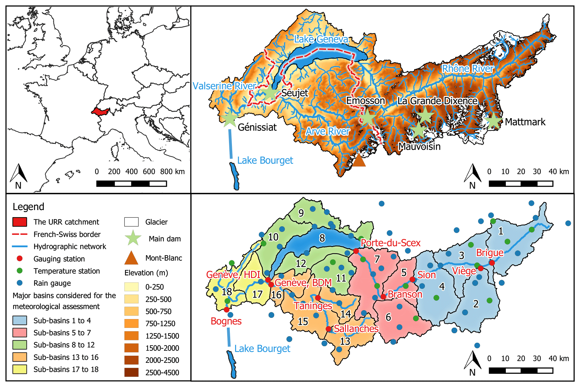
Figure 1Study area. Top panels: localisation and hydrological characteristics of the upper Rhône River (URR) catchment. Bottom panels: locations of the different weather and gauging stations. Genève, HDI: Genève, Halle-de-l'Ile. Genève, BDM: Genève, Bout-du-Monde.
The URR catchment (10 900 km2) covers the south-western part of the Swiss Alps and a part of the northern French Alps (Fig. 1). The altitude of this catchment ranges from 300 to above 4800 m at the top of Mont Blanc. The presence of steep slopes makes this area particularly prone to natural hazards such as landslides, floods, and avalanches, which are strongly connected to meteorological conditions (Beniston, 2006; Raymond et al., 2019).
In this region, the climate is continental and the temporal variability of the precipitation and temperature is high. Mean annual precipitation ranges from 600 mm (in some parts of Wallis canton, Switzerland) to 1100 mm (Chamonix, France). It rains for 30 % to 45 % of the days, with annual maximum daily precipitation reaching locally 45 to 105 mm d−1 on average (Isotta et al., 2014). Glaciated areas covered 17 % of the catchment upstream to Lake Geneva and 10 % of the whole URR catchment in 2015 (GLIMS, 2015).
The gauging station of Bognes (Rhône@Bognes hereafter) records daily mean discharges at the outlet of the URR catchment. It is located at Injoux-Génissiat (France), 46 km downstream of the confluence of the Rhône and Arve rivers. Before the confluence of the two rivers, the hydrological regime of the URR catchment is glacio-nival: the important seasonal snowpack dynamics, combined with the late summer contribution of glacier melt, result in a strong seasonality of flow. Flood events are observed in spring due to snowmelt and in late summer (autumn) due to events with large to very large rainfall amounts (e.g. the so-called Binn—Simplon situations; OFEG, 2002). The URR hydrological regimes become pluvio-nival downstream with the successive contributions of lower-elevation areas, especially those of the Arve River. Flood events from the Arve River mainly result from extreme rainfall events in autumn (e.g. the so-called “retour d'Est events”; Metzger, 2023).
Upstream to Lake Geneva, the URR hydrological regime is considered to be natural until the 1950s, before the construction of several large seasonal water reservoirs mainly used for hydroelectricity production and flood protection. The reservoirs store the snowmelt and glacier melt inflows from high-elevation areas in spring and summer for hydroelectricity production in winter. The total storage capacity of all reservoirs in the catchment is 1200×106 m3 or roughly 20 % of the annual catchment precipitation. Since the 1950s, the URR hydrological regime has thus been significantly altered, with a reduced seasonality (higher river discharges in winter, smaller ones in spring and summer) and reduced flood discharges in summer and autumn (Hingray et al., 2014). Downstream, Lake Geneva, which is the largest natural water reservoir in western Europe (580 km2), has a significant natural buffer effect on river flows. Its influence on flows has even been exacerbated since 1884 with the construction of a downstream regulation weir for flood protection and hydroelectricity production (Grandjean, 1990).
3.1 Meteorological and hydrological data
The density of weather stations covering the URR catchment is rather high. Daily meteorological variables are available from 1 January 1961 to 31 December 2015 for 62 rain gauges and 39 temperature stations in the catchment and in the areas bordering it. The period for which observed daily discharges are available depends on the gauging station. It covers up to 100 years for the URR at Rhône@Porte-du-Scex, the outlet of the river to Lake Geneva (Fig. 2). Note that, for some sub-basins, there are no observed meteorological data concomitant with “natural” discharge data. Weather and hydrological data were provided by (i) the Office Fédéral de l'EnVironnement (OFEV) for the Swiss part and (ii) Météo France and Banque Hydro for the French part. The observed level of Lake Geneva has also been available from the OFEV since 1886 at a daily time step.
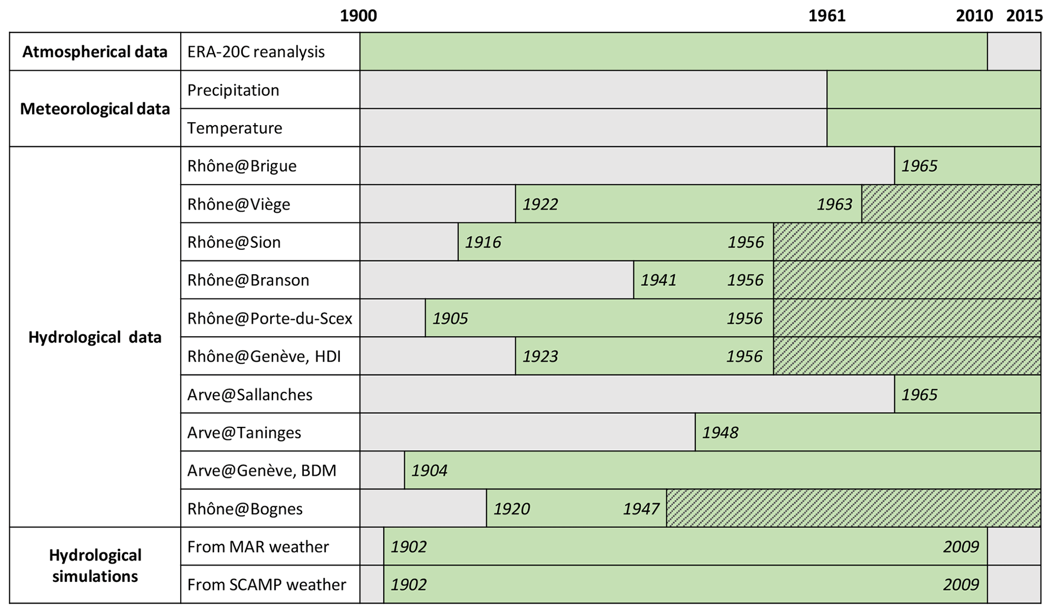
Figure 2Data used. Periods for which daily variables are available are shown in green. Hatchings indicate periods for which the hydrological regime of the URR catchment is significantly altered by dams. Rhône@Genève, HDI: Rhône@Genève, Halle-de-l'Ile. Arve@Genève, BDM: Arve@Genève, Bout-du-Monde. MAR: dynamical downscaling model. SCAMP: statistical downscaling model.
3.2 Atmospheric data
The global atmospheric reanalysis ERA-20C from the European Centre for Medium-Range Weather Forecasts (ECMWF; Poli et al., 2016) is used (i) as a boundary condition for the dynamical downscaling model MAR and (ii) directly as input for the statistical downscaling model SCAMP. This reanalysis provides 6-hourly data over the 1900–2010 period at a 1.25° spatial resolution for a number of atmospheric variables (e.g. geopotential height, wind speed, temperature, or humidity of air masses). The URR catchment is covered by eight ERA-20C grid points.
4.1 Modelling chains
The modelling chains developed in this study are made up of (i) a downscaling model, either dynamical (MAR) or statistical (SCAMP), to generate time series scenarios of regional weather from the global atmospheric reanalysis ERA-20C, and (ii) the glacio-hydrological model GSM-SOCONT, to simulate the corresponding discharge time series scenarios at different gauging stations in the URR catchment.
In this work, we also assess the need for a bias correction of the downscaled weather scenarios prior to their use for hydrological simulations. In some of the configurations considered in the following, a bias correction step is additionally included in the modelling chains. This applies to precipitation, temperature, and temperature lapse rates.
The different models considered in the simulation chains are described below, in Sect. 4.2 for the hydrological model, in Sect. 4.3 for the dynamical and statistical downscaling models, and in Sect. 4.4 for the bias correction model. Section 4.5 sums up the different experiments carried out with these modelling chains.
4.2 Hydrological model
4.2.1 The GSM-SOCONT model
The discharge simulations were performed with a semi-distributed and daily configuration of GSM-SOCONT (Schaefli et al., 2005), a bucket-type model that uses time series of mean areal precipitation and temperature as inputs for each hydrological unit (see Fig. S1 in the Supplement). The URR catchment is divided into 18 sub-basins. They were selected so that they are roughly the same size and that a gauging station is located at the outlet of a sub-basin wherever possible (Obled et al., 2009). The ice-covered and ice-free parts of each sub-basin, extracted from Global Land Ice Measurements from Space (GLIMS, 2015), are considered separately and divided into 500 m elevation bands.
For each elevation band, further referred to as a relatively homogeneous hydrological unit (RHHU), daily mean areal precipitation and temperature are estimated from neighbouring weather stations using Thiessen's weighting method and a regional and time-varying temperature–elevation relationship (Hingray et al., 2010). The choice of Thiessen’s weighting method is discussed in Sect. 6.4. Mean areal temperature is estimated for the mean RHHU elevation. Mean areal precipitation is supposed to be solid if mean areal temperature is smaller than a critical temperature Tc1, liquid if mean areal temperature is higher than a critical temperature Tc2, and mixed otherwise. The Tc1 and Tc2 values are fixed to 0 and 2 °C following Hingray et al. (2010) and Froidurot et al. (2014).
For each RHHU, the snowpack temporal evolution is computed based on mean areal precipitation and temperature time series. Each simulation day, solid and/or liquid precipitation is added to the snowpack storage and/or to its liquid water content. The liquid water content is also increased by snowmelt if any exists and the snowpack is increased by refreezing water if any exists. Snowmelt (refreezing water) is estimated with a degree-day model from the positive (negative) temperature degrees of the day. When the liquid water content reaches the snowpack retention capacity, an “equivalent rainfall” is released. The retention capacity is assumed to be proportional to the snowpack water equivalent following Kuchment and Gelfan (1996). For glaciated RHHUs, ice melt can additionally occur, i.e. when the glacier surface is free of snow. Ice melt is also estimated with a degree-day model.
For glaciated RHHUs, the rainfall and meltwater–runoff transformation is completed through two linear reservoirs, one for ice melt and one for the rainfall or equivalent rainfall. For non-glaciated RHHUs, the rainfall or equivalent rainfall is separated into infiltration and effective rainfall. Infiltration feeds a non-linear soil reservoir which produces deep infiltration and sub-surface flow. Infiltration (actual evapotranspiration) is estimated from equivalent rainfall (potential evapotranspiration) and simulated soil moisture. Effective rainfall feeds a linear overland reservoir which produces direct runoff.
Potential evapotranspiration (PET) estimates were derived from PET estimates of the Climate Research Unit (CRU) produced at a 0.5° spatial resolution from a variant of the Penman–Monteith formula (Harris et al., 2014). In order to derive PET estimates for high-elevation RHHUs, PET was assumed to be a linear function of temperature T. The PET–T relationship was estimated for the region on a monthly basis from the CRU PET and T estimates produced for the 1900–2010 period.
The discharge simulated at the outlet of each sub-basin is the sum of the different discharge components produced by the different RHHUs from the glaciated and non-glaciated areas of the sub-basin. Discharges simulated for the sub-basins are summed to produce those at each gauging station and at the catchment outlet. The daily time step used in the simulations and the rather small size of the catchment area allow us to disregard the routing of discharges through the river network.
Seven parameters have to be estimated for each ice-free RHHU (e.g. snowmelt degree-day factor, storage capacity, and recession coefficient of reservoirs). Three additional parameters have to be estimated for glaciated RHHUs (ice melt degree-day factor and recession coefficients of ice and snow reservoirs).
4.2.2 Hydrological model calibration
In most cases (as here), hydrological models simulate the natural behaviour of the considered catchments. One frequent approach for estimating the model parameters in such a configuration requires a time period with concomitant observations of weather and natural discharges, i.e. concomitant observations of weather and discharges not altered by anthropic activities or waterworks. For most sub-basins of the URR catchment, there is no such period. Daily weather observations are mainly available from the 1960s (here for the period –2015), whereas their hydrological behaviour was natural until the 1950s only and strongly altered afterwards by dams.
The method used for parameter estimation was thus adapted to the sub-basin data configuration, depending (i) on the “perturbation” level of the sub-basin hydrological behaviour during the period P* and (ii) on the availability of flow observation records for the period prior to the 1950s. For gauged sub-basins for which the hydrological behaviour can be considered natural (or at least not significantly altered) over the period P* (or at least over a significant sub-period P*), parameters were estimated with a classical hydrological calibration approach, minimising an objective function estimated from simulated and observed discharge time series in the same period, i.e.
where NSEchrono is the Nash–Sutcliffe efficiency criterion (Nash and Sutcliffe, 1970) obtained from day-to-day deviations between observed and simulated daily discharges.
For gauged sub-basins for which the hydrological behaviour is significantly altered over P* and for which natural flow observations are available prior to 1950, parameters were estimated based on hydrological signatures (Sivapalan et al., 2003; Winsemius et al., 2009). In the present case, parameters were calibrated so that simulated signatures reproduce at best observed ones, but observed and simulated signatures come from different periods following Hingray et al. (2010) (e.g. 1961–2015 and 1922–1963 respectively for the Viège sub-basin).
The signatures considered here are the interannual daily regime (366 values) and the statistical distribution of the annual daily discharge maxima. The objective function is a combination of the NSE criterion and the Kolmogorov–Smirnov distance dKS, applied respectively between simulated and observed signatures:
where is the Kolmogorov–Smirnov distance with and the corresponding discharge percentiles in the observed and simulated distributions.
For ungauged sub-basins, parameters were obtained via regionalisation, following the methodological recommendations of Bárdossy (2007) and Viviroli et al. (2009). All the ungauged sub-basins located upstream of a given gauging station were calibrated at the same time and forced to share the same parameter set. The discharge time series used for the calibration is the time series simulated with this multiple-sub-basin configuration at the downstream gauging station, where observations are available. The ungauged sub-basins can be seen in Fig. 1. The sub-basins grouped together for the calibration of their parameters are also listed in Table S1 in the Supplement.
In practice, whatever the calibration configuration and the calibration objective function, we used the automatic calibration algorithm DDS (dynamically dimensioned search; Tolson and Shoemaker, 2007). The objective function values and the results of the classical and signature-based calibrations are given for each sub-basin in Table S1 and in Figs. S2 and S3 respectively.
Depending on the available data, we thus considered different calibration approaches. Because of this data context, it is not always easy to assess the relevance of the calibration. For sub-basins where concomitant weather and natural discharge data are available over a sufficiently long period, this assessment can be made with a classical split-sample test. The split-sample tests carried out by Schaefli et al. (2005) for three URR sub-basins show that the classical calibration is efficient and robust in this context.
For sub-basins for which the hydrological behaviour is significantly altered by dams, the split-sample test is not possible, as the data of the entire period have to be considered for the signature-based calibration. The analyses described below nevertheless suggest that the signature-based calibration remains efficient and robust in our context.
To assess this, we recalibrated the parameters of the four URR sub-basins that present a natural (or at least not significantly altered) hydrological regime, using only the hydrological signatures. In a first analysis, the signatures were estimated using the same data (period P0) than those considered for the classical calibration (see Fig. S4). The simulated time series remain in good agreement with the observed ones. The NSE coefficients are logically lower than those obtained with the classical calibration approach, but the differences are quite small (see Fig. S5).
In a second analysis, we carried out a similar split-sample test for the signature-based calibration. To do this, we split the period into two (sub-periods P1 and P2), we recalibrated the parameters using only the hydrological signatures of period P1 with the weather data from P1 and, with this set of parameters, we simulated over period P2 the discharge time series from the weather data of P2. The simulated time series remain in good agreement with those observed. They are also in good agreement with those obtained with a signature-based calibration when signatures are derived from the entire period P0. The NSE coefficients are logically lower, but the differences are quite small (see Fig. S6).
4.2.3 Modelling the behaviour of Lake Geneva
An ad hoc model was developed to simulate the influence of Lake Geneva on river flows. The lake has a natural buffer effect on flows, additionally altered with its regulation. From the 1990s, the outflows follow the main regulation objectives of the 1997 settlement (CERCG, 1997), i.e. (i) a target water level in the lake for each calendar day, (ii) the environmental low flow to be satisfied downstream and (iii) the discharge to not be exceeded except during periods of high water in the lake. The day-to-day variations in lake outflows are additionally driven by the hydroelectric production required from the plant at the lake outlet to satisfy a part of the regional electricity demand.
Because of a lack of appropriate data, here we only accounted for the natural buffer effect of the lake and for the main regulation objectives mentioned above. The natural buffer effect is simply modelled with the classical three-equation system needed to simulate the behaviour of unregulated reservoirs, i.e. a water balance, a water level storage and a reservoir flow equation (Hingray et al., 2014). Here, a simple linear water level–storage relationship is considered and the outflow that would be obtained without regulation is assumed to be proportional to the volume stored in the reservoir. For the water balance, changes in storage are obtained each day from reservoir inflows (direct precipitation and upstream and lateral basin flows) and losses (evaporation, lake outflow), where evaporation is estimated with Rohwer's equation (Rohwer, 1931).
4.3 Downscaling models
4.3.1 The dynamical downscaling model MAR
MAR (Gallée, 1995; Gallée and Schayes, 1994; Gallée et al., 1996) is a hydrostatic primitive equation model for regional atmospheric simulations. It includes a detailed scheme of cloud microphysics with six prognostic equations for specific humidity, cloud droplet concentration, cloud ice crystals (concentration and number), and concentrations of precipitating snow particles and raindrops. The convective adjustment is parameterised according to Bechtold et al. (2001). MAR is coupled to the one-dimensional land surface scheme SISVAT (Soil Ice Snow Vegetation Atmosphere Transfer; De Ridder and Schayes, 1997; Gallée et al., 2001) that includes a snow multi-layer scheme (Brun et al., 1992; Gallée and Duynkerke, 1997).
First designed for polar regions, especially Antarctica and Greenland (e.g. Gallée et al., 1996), MAR was also applied over other regions worldwide, such as mid-latitude areas (e.g. Wyard et al., 2017; Doutreloup et al., 2019), mountainous areas (e.g. Himalaya; Ménégoz et al., 2013) and western Africa (e.g. Chagnaud et al., 2020). For the present study, we used the MAR simulation forced by the global atmospheric reanalysis ERA-20C over the 1902–2009 period and produced at a 7 km resolution over the European Alps (Ménégoz et al., 2020a; Beaumet et al., 2021). The URR catchment is covered by 281 MAR grid points.
4.3.2 The statistical downscaling model SCAMP
SCAMP (Raynaud et al., 2020) is a statistical downscaling model based on atmospheric analogues (Lorenz, 1969). It assumes that similar large-scale atmospheric configurations lead to similar local or regional weather situations (e.g. Obled et al., 2002; Chardon et al., 2014). The simulation process is partly stochastic: for each simulation day, 1 of the 30-nearest analogues is randomly selected and used as a weather scenario for this day. SCAMP can thus be used to generate multiple weather scenarios. In the present work, SCAMP was used to generate 30 time series of daily spatial weather scenarios for the 1902–2009 period from the global atmospheric reanalysis ERA-20C outputs. The simulation process is described in the following and summarised in Fig. 3.
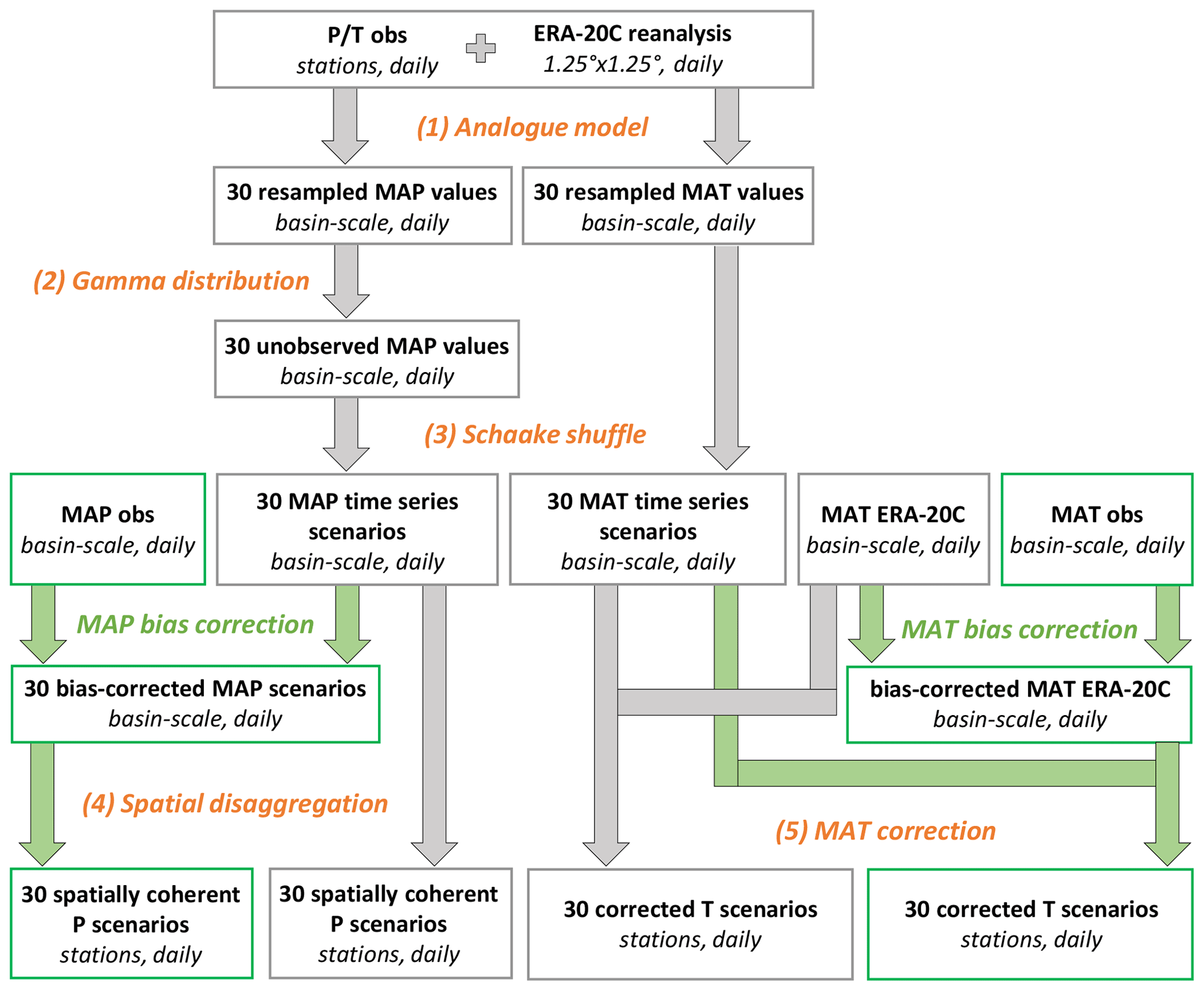
Figure 3Scheme of the statistical downscaling model SCAMP. Orange: components used in the SCAMP simulation. Green: additional components used in the SCAMP bias-corrected simulation. Bold: outputs obtained after each step. Italics: spatial and temporal resolutions. P: precipitation. T: temperature. MAP: mean areal precipitation. MAT: mean areal temperature.
-
For each day of the simulation period, the 30-nearest atmospheric analogue days are identified from candidate days available in the archive period (1961–2009 in the present case). The candidate days are the days found within a 61 d calendar window centred on the target day. A two-step analogue selection is considered. The 100-nearest analogues in terms of large-scale atmospheric circulation are first identified. The selection criterion is the Teweles–Wobus score (Teweles and Wobus, 1954) applied to the daily geopotential heights at 1000 and 500 hPa. It quantifies the similarity between fields from their shapes, thus informing the origin of the air masses. The 30-nearest analogues are sub-selected from these 100-nearest analogues, based on small-scale atmospheric features following Raynaud et al. (2020), i.e. 600 hPa vertical velocities and large-scale temperature at 2 m from September to May (large-scale precipitation otherwise).
-
Following Chardon et al. (2016), SCAMP is used to generate mean areal precipitation (MAP) and mean areal temperature (MAT) values for the whole URR catchment. To generate weather scenarios with values different from observations, SCAMP extends the analogue method with a random generation process from a day-to-day adjusted statistical distribution (Chardon et al., 2018; Raynaud et al., 2020). For precipitation, a Gamma distribution is fitted each day to the 30 regional MAP values obtained for the whole URR catchment from the analogues. The distribution is then used to generate a new sample of 30 regional MAP values, i.e. unobserved (and possibly higher than observations). This adaptation was shown to improve the simulation of maximum regional MAP accumulations (Raynaud et al., 2020, Fig. 8 therein).
-
Thirty regional MAP and MAT time series scenarios are produced from the 30 regional MAP and MAT values generated each day. To improve the temporal consistency between consecutive days in each time series, the 30 regional MAP and MAT scenarios obtained for each day are paired with the 30 scenarios of the previous day with a Schaake shuffle reordering approach (Clark et al., 2004; Raynaud et al., 2020).
-
Following Mezghani and Hingray (2009) and Viviroli et al. (2022), the regional MAP time series scenarios are finally disaggregated with a non-parametric method of fragments to produce spatial MAP time series scenarios for the URR catchment (with one mean areal precipitation value for each RHHU of the hydrological model). In practice, the regional MAP scenario of each day is spatially disaggregated using the spatial pattern of an analogue day for which weather observations are available.
-
The large-scale atmospheric features considered for the identification of the analogues are not as informative for temperatures. The temperature additive correction method of Kuentz et al. (2015) was thus used to make each day of the regional MAT time series scenarios coherent with the regional MAT time series of the global atmospheric reanalysis ERA-20C. For each prediction day and each scenario, the correction factor is the difference between the regional MAT value of the ERA-20C reanalysis and the regional MAT value of the scenario. The correction factor is applied to correct the temperatures of all the stations for this scenario. For instance, if the daily regional MAT value of the scenario is 2 °C warmer than the regional MAT value of the ERA-20C reanalysis, then all local temperatures of the scenario are lowered by 2 °C.
4.4 Bias correction
As shown in Sect. 5.1, the simulated weather scenarios from the dynamical downscaling model MAR and the statistical downscaling model SCAMP can be significantly different from the observations. Corrected precipitation and temperature scenarios are also considered in the following. Quantile mapping bias correction (BC hereafter) was used for both variables and both models (Déqué, 2007). The different regional MAP and MAT time series were corrected using the observed regional MAP and MAT time series as references. As is commonly done, the correction is additive for MAT and multiplicative for MAP, and one BC function was estimated for each calendar month.
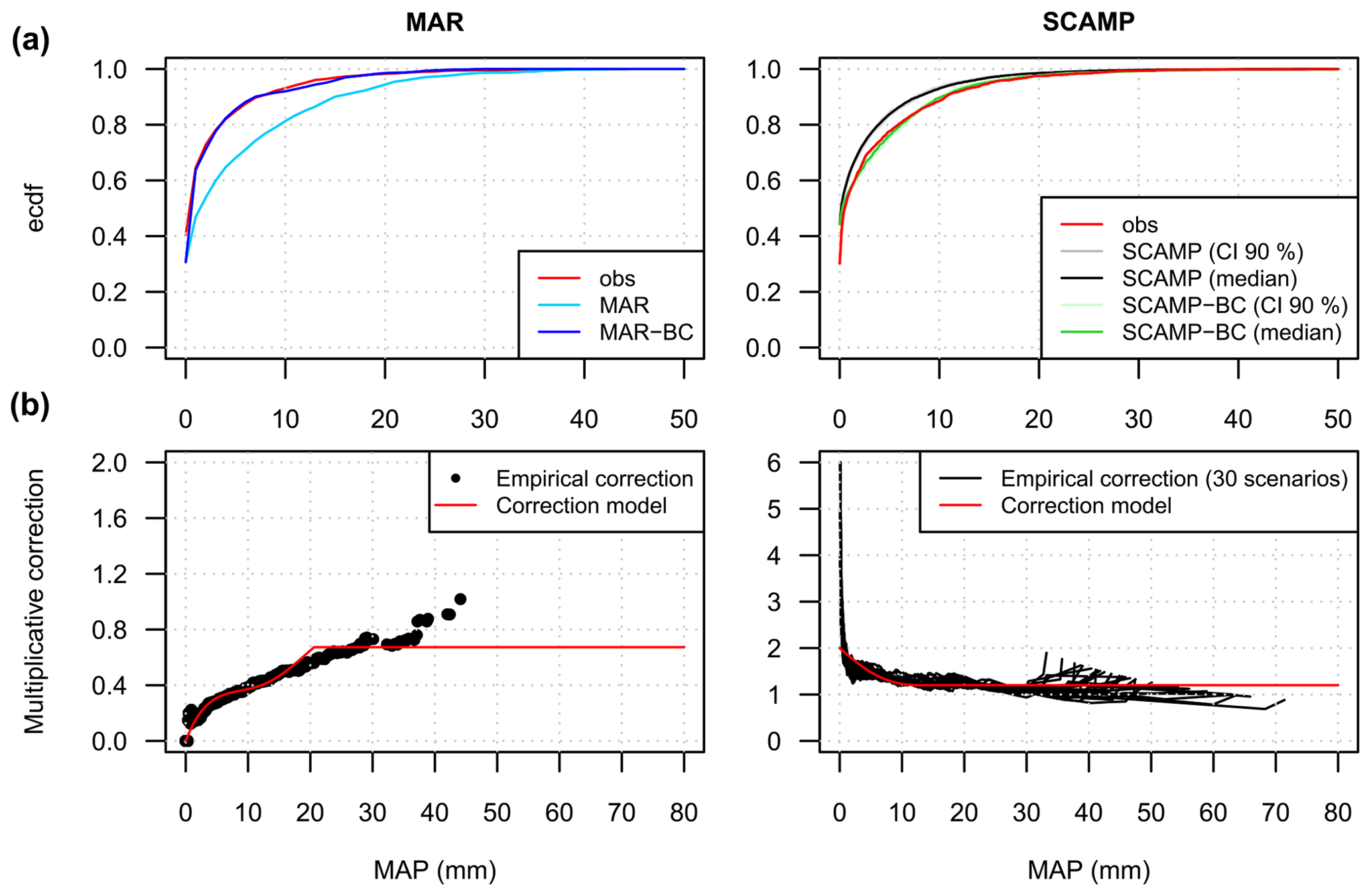
Figure 4Examples of bias correction for MAP. MAR: sub-basins 1 to 4, January. SCAMP: URR catchment, August. Control period: 1961–2009. (a) Empirical cumulative distribution function (ecdf). (b) Correction functions. For SCAMP, the grey and green bands represent the confidence intervals at the 90 % level. The median scenarios are indicated by the black and green solid lines.
For both models, an analytical BC function was used to ease interpolations of correction factors estimated between empirical percentiles (a degree-4 polynomial was fitted to the empirical correction factors). To avoid irrelevant extrapolations of correction factors for extreme MAP values not simulated in the control period, the correction value was bounded. It was bounded for the highest MAP percentiles (95th to 100th percentiles) to their mean empirical correction value. For MAT, the corrections for the lowest (0th to 5th) and highest (95th to 100th) percentiles were similarly set to their mean empirical correction values.
For SCAMP, the MAP and MAT corrections could only be performed at the scale of the whole URR catchment. To keep the small-scale variability between the different scenarios produced by SCAMP, one single BC function was considered for the 30 time series. For MAR, specific BCs were applied for each of the five major sub-basins shown in Fig. 1. Examples of BC functions are shown for MAP in Fig. 4.
Note that, for the MAR simulations, a BC of the temperature lapse rates was also necessary. For hydrological simulations, temperature estimates are required for each elevation band. In the present work, they are obtained by interpolation from temperature values available at neighbouring locations, using a regional temperature–elevation relationship. For the MAR simulations, this relationship is assumed to be linear, and its slope, the so-called “lapse rate”, is estimated for each time step from simulated temperatures using all MAR grid cells in the URR catchment.
As illustrated by its statistical distribution in Fig. 5b, the lapse rate estimated from MAR simulations varies from one day to another, as does the lapse rate estimated from observations. However, it is on average higher than that of the observations, as also illustrated in Fig. 5a with the mean temperature–elevation relationships estimated from both data sets. The bias in the lapse rate, which likely results from a warm bias in the lower-atmospheric layers of the model, is quite large, of the order of 0.3 °C per 100 m (Fig. 5b).
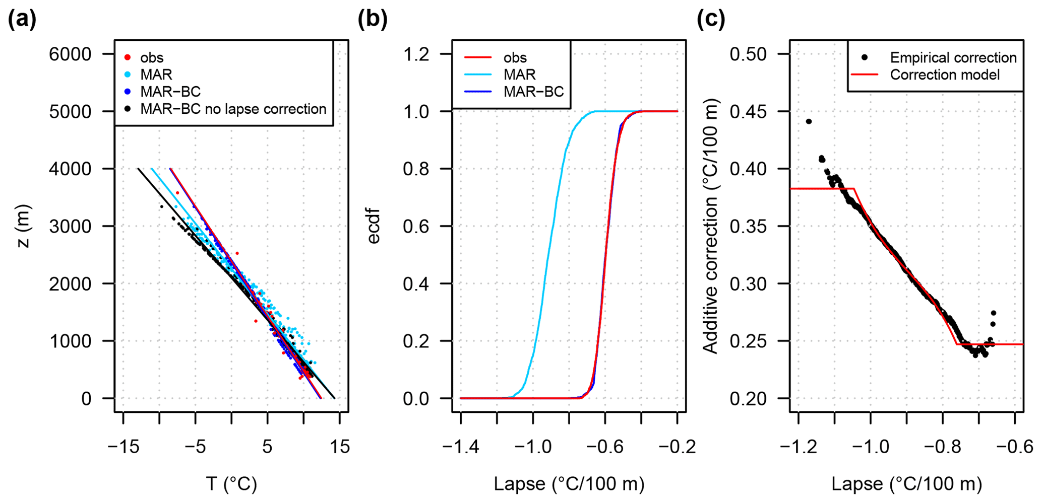
Figure 5Illustration of the bias in the temperature–elevation relationship in the simulations of the dynamical downscaling model MAR. (a) Mean interannual relationship (and corresponding linear regressions) at the catchment scale from observed temperatures (obs, red), raw MAR simulations (MAR, cyan), MAR simulations corrected for bias in mean temperature and lapse rate (MAR-BC, blue), and MAR simulations corrected for bias in mean temperature only (MAR-BC no lapse correction, black). (b, c) Examples of ecdfs and the correction model for the temperature lapse rate (sub-basins 1 to 4, July). Note that the blue and red lines overlap in panels (a) and (b).
The bias in temperature in dynamical downscaling models has been recognised and corrected for a long time. To the best of our knowledge, the bias in the lapse rate has not been. A common approach for using model temperatures for hydrological simulations is to identify the BC function for a given reference altitude and to use this function to correct model temperatures for all other elevations. In this process, however, the lapse rates remain unchanged and the corrected MAT may still present residual biases for all elevations different from the reference one. This is the case for the present work. For the mountainous context considered here, as discussed in Sect. 6.2, this has important implications for the simulated hydrology.
For MAR temperatures, we thus considered a two-part quantile mapping correction function that takes into account both biases, that of the MAT value simulated for a given reference elevation and that of the lapse rate. The corrected MAT value for a given elevation z and a given time t was obtained as follows:
where MATMAR-BC(zref,t) is the bias-corrected MAT value at the reference elevation zref (the correction depends on the percentile of the MAT value at t) and lapseMAR-BC(t) is the bias-corrected lapse rate value at t (the correction depends on the percentile of the lapse rate value estimated from MAR outputs at t).
In practice, we chose the mean elevation of the URR catchment (i.e. 1525 m) as the reference elevation. The MAT and lapse rate corrections were carried out independently at the monthly scale and for the five major basins shown in Fig. 1. The results presented in the following for the MAR simulations were obtained with this two-part BC. The influence of the lapse rate correction is discussed in Sect. 6.2.
Note that, for the SCAMP simulations, a BC of the temperature lapse rates was not necessary. In the SCAMP simulations, the regional temperature–elevation relationship is estimated each day from the SCAMP temperatures at the observation stations. For each simulation day, as these temperatures are derived from the temperatures of an observed analogue day, the relationship of the scenario always corresponds to an observed one. The temperature–elevation relationship and its variations over time are therefore consistent with the observations.
4.5 Experimental setup
Four experiments are considered in the present work. They are summarised in Fig. 6. Weather scenarios are produced with either the dynamical downscaling model MAR or the statistical downscaling model SCAMP from large-scale atmospheric information (ERA-20C data). Weather scenarios obtained with each downscaling model are used to force the GSM-SOCONT model and simulate hydrological scenarios. Weather scenarios are first used with their raw values and then with their bias-corrected values. In the following, the simulations with raw weather scenarios are referred to as “MAR” and “SCAMP” simulations. The bias-corrected simulations are referred to as “MAR-BC” and “SCAMP-BC” simulations. Both weather and hydrological scenarios can be compared to their counterpart references (observed or simulated as explained below). Among other things, we will compare the ability of each hydro-meteorological modelling chain to reproduce the temporal variations in both weather variables and discharges (Table 1).
Table 1Summary of the different hydro-meteorological variables simulated and assessed in this study. MAP: mean areal precipitation. MAT: mean areal temperature. URR: upper Rhône River.
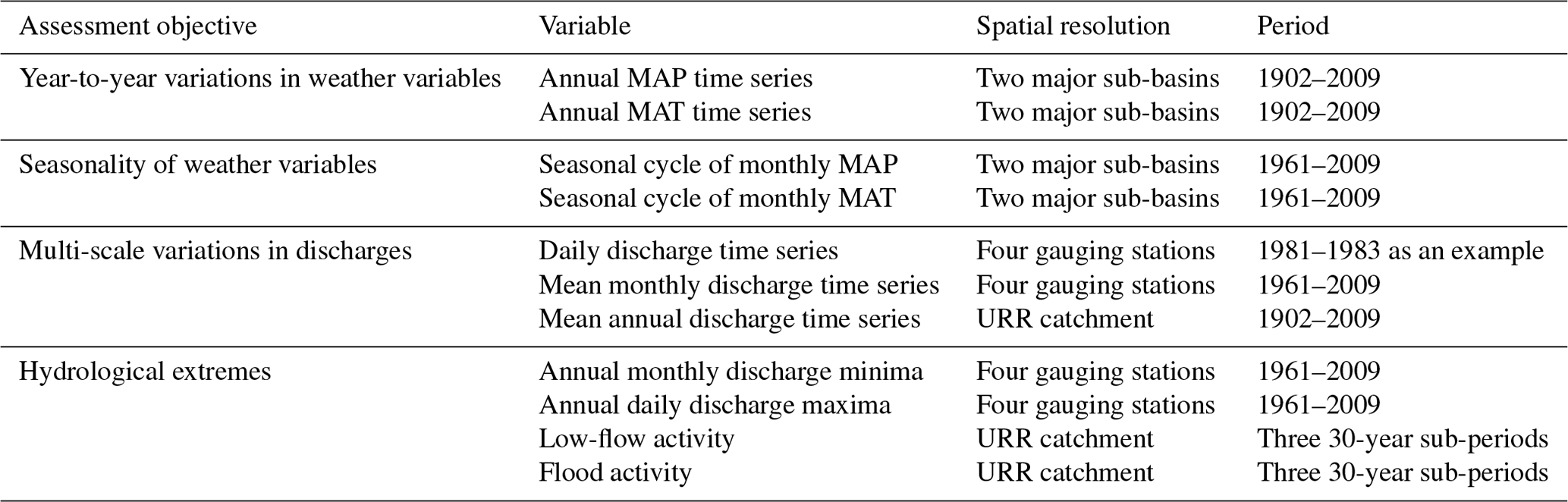
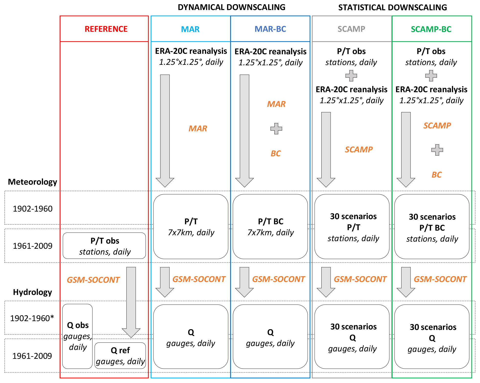
Figure 6Summary of the different experiments. Orange: models used, i.e. MAR (dynamical downscaling model), SCAMP (statistical downscaling model), BC (bias correction model), and GSM-SOCONT (hydrological model). Bold: outputs obtained after each step. Italics: spatial and temporal resolutions. * Time period depending on the considered gauge. obs: observed precipitation or temperature. : simulated precipitation or temperature. BC: simulated bias-corrected precipitation or temperature. Q obs: observed discharge. Q ref: simulated discharge from observed weather variables. Q: simulated discharge.
As many sub-basins have altered hydrological regimes, the “hydrological reference” used for the comparison is the discharge time series obtained via hydrological simulation with the observed weather variables as inputs. For some upstream sub-basins for which the hydrological behaviour can be considered natural, the evaluation could also rely on a comparison with discharge observations. We however chose to use the simulated reference. This first makes the evaluation homogeneous for all URR sub-basins and additionally allows us to focus only on the ability of the downscaling chains to simulate hydrologically relevant weather scenarios. In other words, this allows us to not distort the evaluation by intrinsic errors introduced by the hydrological model. This point is further discussed in Sect. 6.4.
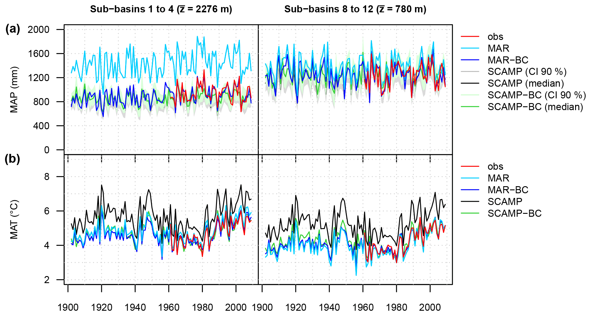
Figure 7Time series of annual (a) MAP and (b) MAT for two major basins (1902–2009). The average elevation of each major basin is indicated in brackets. For MAP, the grey and green bands represent the confidence intervals at the 90 % level. The median scenarios are indicated by the black and green solid lines. For MAT, the 30 SCAMP time series scenarios are identical and correspond to the raw or bias-corrected time series of the ERA-20C reanalysis. obs: observed weather. MAR or MAR-BC: raw or bias-corrected weather scenario produced with the dynamical downscaling model MAR. SCAMP or SCAMP-BC: raw or bias-corrected weather scenarios produced with the statistical downscaling model SCAMP.
A multi-scale evaluation of simulations is carried out. Here we present the meteorological evaluations carried out at the scale of two of the five major sub-basins shown in Fig. 1 and hydrological evaluations at four illustrative gauging stations. Rhône@Porte-du-Scex (gauged area of 5390 km2) is the outlet to Lake Geneva of the upstream part of the URR catchment. Rhône@Genève, Halle-de-l'Ile (7945 km2) is the outlet of Lake Geneva. Arve@Genève, Bout-du-Monde is on the Arve River before its confluence with the Rhône River (1990 km2), and Rhône@Bognes (10 900 km2) is the outlet of the URR catchment.
5.1 Weather
Simulated weather variables are compared to observations in Figs. 7 and 8 for both downscaling models. Figure 7 shows observed and simulated year-to-year variations in annual MAP and MAT and Fig. 8 the seasonal cycles of monthly MAP and MAT. Results are presented for sub-basins in the upper part of the URR catchment (sub-basins 1 to 4; Figs. 7 and 8, left column) and for sub-basins downstream from and around Lake Geneva (sub-basins 8 to 12; Figs. 7 and 8, right column). For the statistical downscaling model SCAMP, both figures present the dispersion between the 30 annual MAP values obtained from the 30 time series scenarios (grey and green bands). Note that the dispersion is rather large for precipitation (e.g. up to 600 mm for annual MAP, Fig. 7), illustrating the important uncertainty in the large-scale–small-scale relationship for this variable in this region.
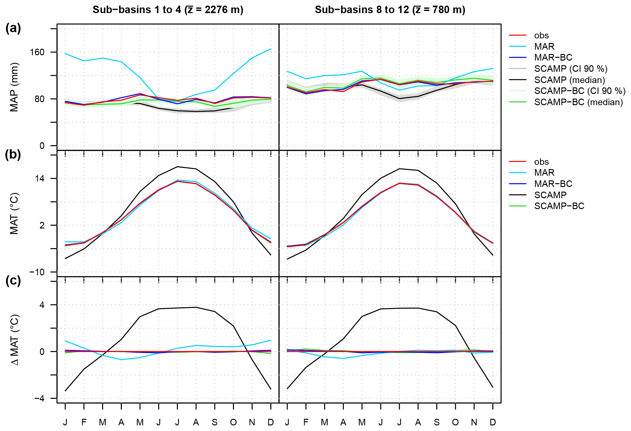
Figure 8Seasonal cycles of (a) MAP and (b, c) MAT for two major basins (1961–2009). The average elevation of each major basin is indicated in brackets. For MAP, the grey and green bands represent the confidence intervals at the 90 % level. The median scenarios are indicated by the black and green solid lines. For MAT, the 30 SCAMP seasonal cycle scenarios are identical and correspond to the raw or bias-corrected seasonal cycle of the ERA-20C reanalysis.
For both downscaling models, simulated year-to-year variations in annual MAP and MAT are in good agreement with observed ones, whatever the area considered (Fig. 7). The positive trend in temperature starting in 1980 is also adequately reproduced, resulting from the global combination of the warming related to anthropogenic greenhouse gases and the reduced anthropogenic aerosol cooling (Reid et al., 2016), which are especially pronounced over Europe (Nabat et al., 2014). However, the mean simulated variables can be rather different from the observed ones. For the dynamical downscaling model MAR, for instance (cyan lines), simulated annual MAPs are 12 % higher than observations for sub-basins around the lake and 58 % higher for sub-basins in the upper part of the URR catchment. For the statistical downscaling model SCAMP (grey bands and black lines), the differences, although much smaller, are still significant. Depending on the SCAMP scenario, simulated annual MAPs are 2 % to 8 % smaller than observations around the lake and 10 % to 15 % smaller for the upper part of the URR catchment. Some differences are also obtained for annual MATs. They are small for MAR (0.1 °C around the lake, 0.3 °C in the upper part of the URR catchment). For SCAMP, the simulations are roughly 1 °C warmer for the whole area (black lines).
As shown in Fig. 8, the deviations from observations can vary a lot from one season to another. In the upper part of the URR catchment, precipitation amounts simulated with MAR are similar to observations in summer but much larger in autumn and spring (+56 % and +71 %) and even larger in winter (+110 %). Around the lake, simulated precipitations are almost similar to observations in autumn (+8 %) and summer (−7 %) but are again significantly larger in winter and spring (+24 %). For SCAMP scenarios, differences are almost exclusively found in summer, when simulated MAPs are 15 % to 30 % smaller than observations for the whole area. A significant seasonality of the deviations is also found for MATs. For MAR, the difference is −0.7 °C in spring and up to +1.1 °C in winter. For SCAMP, the seasonality is even larger: simulations are up to 3.7 °C warmer than observations in summer and, conversely, up to 2.7 °C colder in winter.
For both models, the differences mentioned above are significantly reduced and sometimes vanish completely after BC (blue lines for MAR-BC and green bands or solid lines for SCAMP-BC). This is the case for annual variables (Fig. 7) but also for monthly variables (Fig. 8) as the BC is performed on a monthly basis. For SCAMP, as the BC is performed at the catchment scale, some biases can remain at the sub-basin scale. For annual MAPs, for instance, simulations are still 3 % to 9 % smaller than observations in the upper part of the URR catchment and 0 % to 6 % larger around the lake, depending on the scenario (Fig. 7).
5.2 Discharge seasonality and variations
The discharges obtained via hydrological simulation from weather scenarios are compared with their reference counterparts, i.e. with the discharges obtained via hydrological simulation from observed weather variables. The comparison is applied to time series of discharges at daily, monthly and annual resolutions and to time series of characteristic discharge variables (i.e. minimum monthly discharge observed each year and annual maximum daily discharge). Note that, for SCAMP and SCAMP-BC simulations, for which 30 time series scenarios are simulated, the value of the reference discharge variable considered for a given time is compared to the 30 values obtained for that time from the 30 scenarios.
At a daily time step, the discharge time series of the MAR-BC and SCAMP-BC simulations are in good agreement with the reference ones, as shown by the results obtained for the four illustrative gauging stations in Fig. 9. The agreement is even larger for time series of mean monthly discharges (Fig. 11, left column). The large seasonality of flows as well as their daily and monthly temporal variations are reproduced well, especially for the Rhône River upstream of Lake Geneva. These results are obtained for almost all the gauging stations, even those located downstream of Lake Geneva, despite the significant influence of the lake regulation on flows and the rather crude regulation model used for its representation (Fig. 9e).
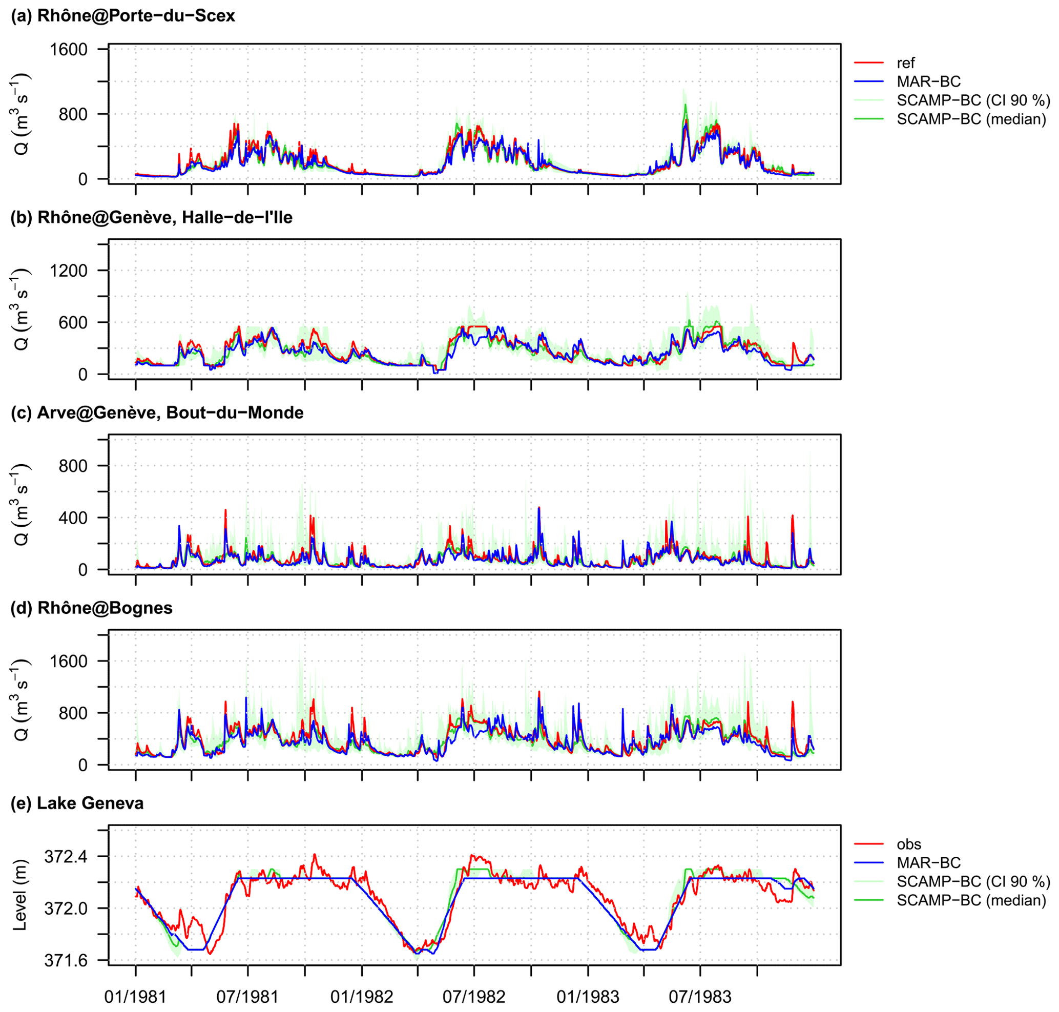
Figure 9Time series of daily discharges at (a) Rhône@Porte-du-Scex, (b) Rhône@Genève, Halle-de-l'Ile, (c) Arve@Genève, Bout-du-Monde and (d) Rhône@Bognes for the 1981–1983 period. (e) Time series of daily levels of Lake Geneva for the same period. The green bands represent the confidence intervals at the 90 % level. The median scenarios are indicated by the green solid lines. ref: simulated discharge from observed weather variables. MAR-BC: simulated discharge from the bias-corrected weather scenario produced with the dynamical downscaling model MAR. SCAMP-BC: simulated discharge from the bias-corrected weather scenarios produced with the statistical downscaling model SCAMP. obs: observed levels of Lake Geneva.
For both downscaling models, the BC of the weather scenarios significantly improves the simulations (Fig. 9 versus Fig. 10, Table 2). The BC is required for both precipitation and temperature variables. This is especially visible in the results obtained for the upstream URR catchment. At Rhône@Porte-du-Scex (Fig. 10a), the discharge variations are reproduced rather well with raw weather scenarios, but the discharges are overestimated with SCAMP and underestimated with MAR during the spring and summer. These deviations may be surprising, as raw SCAMP and MAR precipitation simulations are biased toward not enough summer precipitation in SCAMP and, conversely, much higher winter, spring and autumn precipitation in MAR (Fig. 8). They actually derive from temperature scenarios that are too warm in SCAMP in summer and not warm enough in MAR. This point is discussed further in Sect. 6.2.
Table 2Performance assessment of the modelling chains for the 1961–2009 period. For the dynamical downscaling model (MAR or MAR-BC), the NSE coefficient is calculated from the reference and simulated discharge time series at each gauging station. For the statistical downscaling model (SCAMP or SCAMP-BC), the statistical-index CRPSS (continuous ranked probability skill score; Chardon et al., 2014) is used for the evaluation. For each gauging station, the CRPSS compares the probabilistic predictions of discharge obtained for each simulation day from (i) the climatological distribution and (ii) the 30 simulated time series scenarios. For a perfect model, NSE = 1 and CRPSS = 1. For a model worse than the climatology, NSE < 0 and CRPSS < 0.
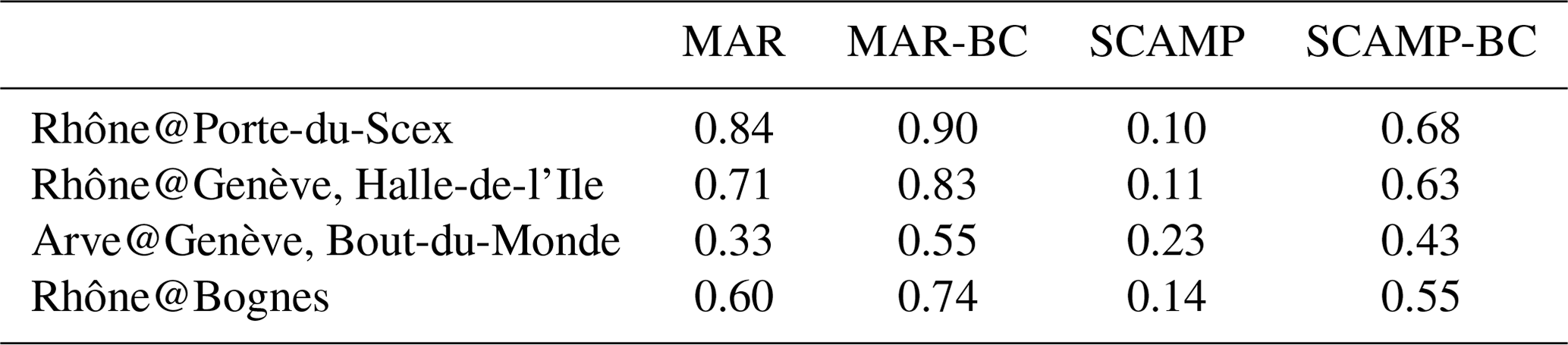
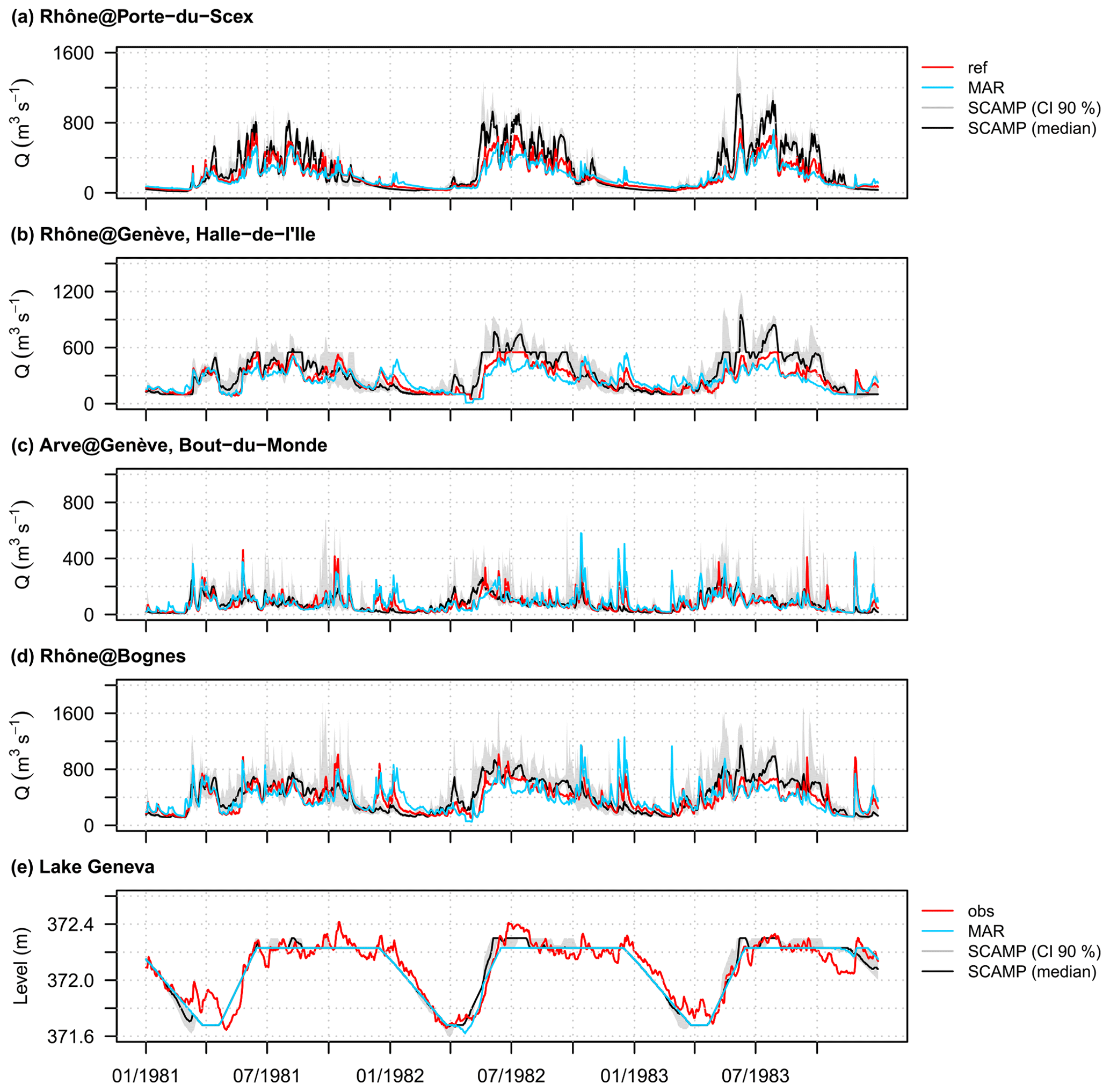
Figure 10Time series of daily discharges at (a) Rhône@Porte-du-Scex, (b) Rhône@Genève, Halle-de-l'Ile, (c) Arve@Genève, Bout-du-Monde and (d) Rhône@Bognes for the 1981–1983 period. (e) Time series of daily levels of Lake Geneva for the same period. The grey bands represent the confidence intervals at the 90 % level. The median scenarios are indicated by the black solid lines. ref: simulated discharge from observed weather variables. MAR: simulated discharge from the raw weather scenario produced with the dynamical downscaling model MAR. SCAMP: simulated discharge from the raw weather scenarios produced with the statistical downscaling model SCAMP. obs: observed levels of Lake Geneva.
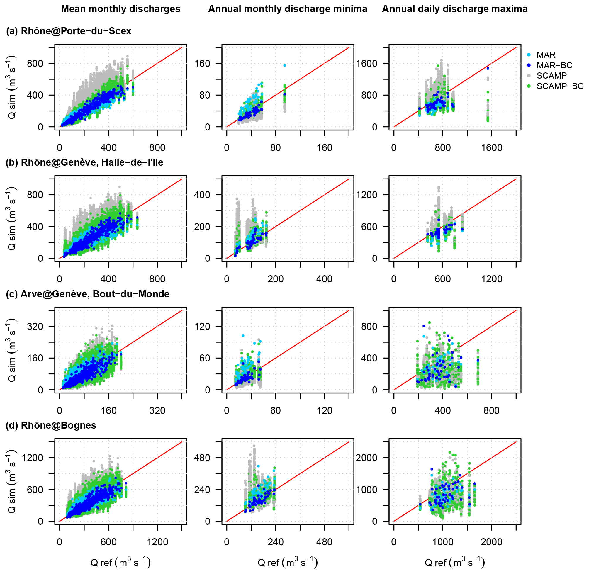
Figure 11Scatter plots of mean monthly discharges, annual monthly discharge minima and annual daily discharge maxima at (a) Rhône@Porte-du-Scex, (b) Rhône@Genève, Halle-de-l'Ile, (c) Arve@Genève, Bout-du-Monde and (d) Rhône@Bognes for the 1961–2009 period. Q ref: simulated discharge from observed weather variables. MAR or MAR-BC: simulated discharge from the raw or bias-corrected weather scenario produced with the dynamical downscaling model MAR. SCAMP or SCAMP-BC: simulated discharge from the raw or bias-corrected weather scenarios produced with the statistical downscaling model SCAMP.
5.3 Floods and low flows
The hydrological relevance of simulated weather scenarios is further evaluated with simulations of floods and low flows. Note that the annual daily discharge maxima are used as flood proxy indicators and that the annual monthly discharge minima are used as low-flow proxy indicators. Figure 11 (middle and right columns) presents scatter plots of simulated and reference values of annual monthly discharge minima and annual daily discharge maxima obtained for the 49 years of the 1961–2009 period. The same figure with results for the first half of the century is given in Fig. S7. For annual monthly discharge minima, the month with the lowest monthly flow in the reference discharge series is identified for each year of the period. The 49 lowest monthly flows are compared to their simulated counterparts for the same months. For annual daily discharge maxima, a similar comparison is made: for each year, the day with the highest reference daily flow is identified, and the corresponding discharge is compared to the maximum daily discharges obtained around that day in the simulations. The maximum discharge considered for the comparison in the simulation is identified from a 7 d window centred on the reference day.
For all the gauging stations, the MAR-BC simulation leads to very satisfactory results for the annual monthly discharge minima. By contrast, the annual daily discharge maxima tend to be underestimated (at Rhône@Porte-du-Scex, Rhône@Genève, Halle-de-l'Ile and Rhône@Bognes) or poorly simulated (at Arve@Genève, Bout-du Monde). For the SCAMP-BC simulations, the annual monthly discharge minima and the annual daily discharge maxima are characterised by a very large inter-scenario variability, making the interpretation of these results more difficult. For annual monthly discharge minima, the medians of simulated scenarios are close to the reference ones at all the gauging stations. For annual daily discharge maxima, the medians are also close to the reference values at Rhône@Porte-du-Scex. They are, however, off-centre downwards for the other three stations. The least well-reproduced annual daily discharge maxima are those of the Arve basin and those at Rhône@Bognes. Conversely to the upper part of the URR catchment, the annual daily discharge maxima occur mainly in late summer and autumn (see Fig. S8). The MAR-BC and SCAMP-BC simulations may thus fail to reproduce the large rainfall amounts in that season, especially convective events, which are known to generate the largest autumn floods in this area.
For annual daily discharge maxima and annual monthly discharge minima, the added value of a BC for weather scenarios is again important (Fig. 11). Depending on the hydrological variable considered, the added value of a temperature BC is not necessarily equivalent to that of a precipitation BC. In the upstream parts of the URR catchment, for instance, low flows occur mainly in winter, due to the low temperatures in this season. The quality of simulated winter low flows thus depends to a great extent on the quality of temperature scenarios and much less on the quality of precipitation scenarios. Conversely to precipitation corrections, temperature corrections therefore lead to a significant improvement in low-flow simulations. This is illustrated by the additional analyses presented in the Discussion section (Sect. 6.2).
5.4 Mean annual discharges and flood and low-flow activities
The modelling chains considered previously are commonly used for hydroclimatic projections with large-scale atmospheric GCM outputs as forcing variables. The potential impact of climate change on hydrology is often assessed by considering changes in the statistical characteristics of hydrological regimes (e.g. changes in seasonality and year-to-year variability, changes in flood and low-flow activities). We therefore also assess the ability of the considered modelling chains to simulate the “reference” variations in different characteristics of the URR hydrological regime over the last century (1920–2009). In this section, as no better reference time series is available, the “references” are observed discharges for the 1920–1960 period and simulated discharges from observed weather variables for the 1961–2009 period. The results are therefore to be interpreted with caution.
The simulated year-to-year variations in mean annual discharges are first compared to the reference ones over the 1920–2009 period (Fig. 12c and d). Due to the large interannual variability of discharges, it would be rather difficult to assess the ability of the modelling chains to catch any long-term trends in this variable. However, the year-to-year variations are reproduced well in both timing and amplitude, especially for the second half of the century. Recall especially that the hydrological model does not alter the comparison during this sub-period, as the two time series compared are obtained by hydrological simulation.
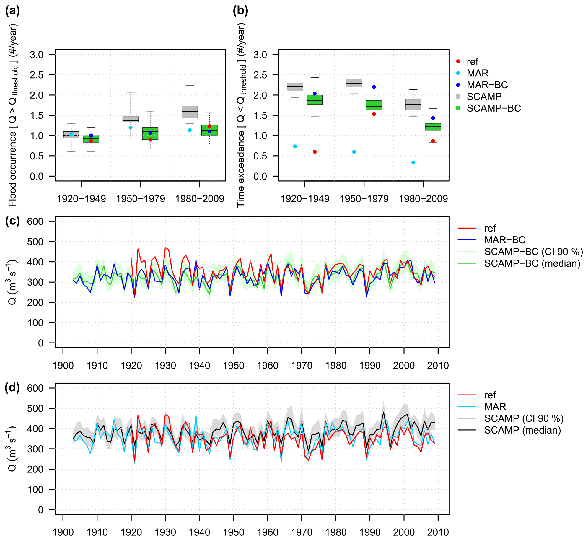
Figure 12(a) Flood activity and (b) low-flow activity at Rhône@Bognes for three 30-year sub-periods: 1920–1949, 1950–1979, and 1980–2009. See the text for definitions of flood activity and low-flow activity. (c) Mean annual discharge time series at Rhône@Bognes for the 1902–2009 period simulated with MAR-BC and SCAMP-BC. (d) The same for simulations with MAR and SCAMP. The grey and green bands represent the confidence intervals at the 90 % level. The median scenarios are indicated by the black and green solid lines. As no better reference time series is available, note that the “references” are observed discharges for the 1920–1960 period and simulated discharges from observed weather variables for the 1961–2009 period. MAR or MAR-BC: simulated discharge from the raw or bias-corrected weather scenario produced with the dynamical downscaling model MAR. SCAMP or SCAMP-BC: simulated discharge from the raw or bias-corrected weather scenarios produced with the statistical downscaling model SCAMP.
We then consider the variations in flood and low-flow activities of the URR catchment. Flood activity is defined here as the average number of daily discharges per 30-year period above a given daily discharge threshold. Low-flow activity is similarly defined as the average number of months per 30-year period during which the mean monthly discharge is below a given discharge threshold. The thresholds retained are the reference discharge values exceeded on average once a year over the entire 90-year simulation period (1920–2009). For flood activity, the threshold was calculated by considering the 90 largest daily discharges over the 90-year period. If the threshold was exceeded several times during 5 consecutive days, only the date of the maximum discharge was retained. For low-flow activity, the threshold corresponds to the 10th percentile, i.e. the 90 lowest values of mean monthly reference discharges over the 90-year period. At Rhône@Bognes, the thresholds are respectively 962 m3 s−1 for floods and 167 m3 s−1 for low flows. The flood and low-flow activities, estimated for each of the three 30-year sub-periods 1920–1949, 1950–1979 and 1980–2009, are presented in Fig. 12a and b.
In both BC simulations, the number of flood events exceeding the threshold and the variations in flood activity from one sub-period to another are in good agreement with the reference ones. The observed increase in flood activity is reproduced rather well (Fig. 12a). The results for low-flow activity are less satisfactory (Fig. 12b). On the one hand, the number of mean monthly discharges below the threshold is, whatever the sub-period, significantly higher than that of the reference. This is more than 3 times higher for the 1920–1949 sub-period. This overestimation is mainly due to longer winter low-flow durations (not shown). On the other hand, the variations in low-flow activity from one sub-period to another are only partially reproduced. While the small decrease observed between the last two sub-periods is captured rather well, the large increase between the first two sub-periods is fully missed. The reasons for this are unclear. The large differences obtained with the raw and bias-corrected downscaling simulations suggest that some limitations remain in the bias-corrected weather scenarios (e.g. too low simulated winter temperatures). The large differences in the reference low-flow activity obtained between the sub-periods also suggest an issue with the stationarity assumption (e.g. hydrological signatures) and/or the low temporal homogeneity of the data set considered in this work (e.g. the reference discharge time series made from observed or simulated discharges for the beginning and end of the period). These points will be worth investigating further in future works.
All in all, and as already illustrated in a number of previous works (e.g. Boé et al., 2007; Kuentz et al., 2015; Bonnet et al., 2017; Caillouet et al., 2017; Weber et al., 2021), hydrologically relevant weather scenarios (or reconstructions) can be achieved with either statistical or dynamical downscaling models from large-scale atmospheric information only. As also illustrated here, this may require some preliminary BCs to atmospheric model outputs.
As discussed in the following, the need for corrections can be attributed to some limitations of the models. It may also be attributed to the quality of the available “observations”. We will discuss issues related to reanalysis data and to lapse rates for both temperature and precipitation. We will also discuss some issues related to the hydrological model considered in the modelling chains.
6.1 Reanalysis data
The global atmospheric reanalysis ERA-20C considered in this study is used as a pseudo observation of the state and dynamics of the atmosphere over a large spatial area covering the European domain. As it is produced by assimilating only sea level pressure and wind measurements, ERA-20C data are not, however, free of limitations. The quality of the geopotential at 500 hPa and of other large-scale variables (such as vertical velocities at 600 hPa, temperature at 2 m and large-scale precipitation) may be rather low and may impact the skill of both downscaling models.
This is the case, for instance, for the regional MAT time series used to force the SCAMP time series scenarios. The large bias in the regional MAT SCAMP scenarios highlighted in Figs. 7 and 8 directly derives from the bias in the regional MAT of the ERA-20C reanalysis over the considered domain. Similar limitations were reported by Bonnet et al. (2017), who had to correct the biases of a downscaled version of the ERA-20C reanalysis to simulate realistic mean river flows in France.
As shown by Horton and Brönnimann (2019), using a reanalysis assimilating more data, such as the recent ERA5 reanalysis (Hersbach et al., 2020), could lead to more relevant weather scenarios. Such reanalyses were not used in the present work, as they generally cover a much shorter period (around 60 years), preventing the simulation and evaluation of hydro-meteorological scenarios over a century.
6.2 Temperature lapse rate
As shown in Sect. 4.4 (Fig. 5a), the lapse rates estimated from MAR simulations are on average higher than those estimated from observations. For the mountainous context considered here, this bias has important implications for the simulated hydrology. A higher lapse rate leads to lower temperatures than those observed for high-elevation bands in particular (where few observations are available) and vice versa for low-elevation bands. This logically makes the simulated snowpack dynamics significantly different from the observed one. Lower temperatures lead to more frequent solid precipitation, more snow accumulation, less snowmelt in spring and snow cover for longer durations and over larger areas. For the highest-elevation bands, lower temperatures can even lead to a simulation of a perennial snowpack, preventing any simulation of ice melt (which can only occur in the model for elevation bands where the glacier is free of snow). All of this results in poorly simulated hydrological regimes. As already suggested in Sect. 5.4, a biased lapse rate is, for instance, expected to give a poor simulation of winter low-flow characteristics. A higher lapse rate is also expected to lead to delayed snowmelt floods and to low flows in late summer that are not sustained as they should be by ice melt.
If less evident, a biased lapse rate may also give a poor simulation of flood regimes. In the URR catchment, the largest floods often occur in autumn due to large precipitation amounts. In autumn, the temperatures can be low enough for precipitation to fall as snow in high-elevation areas. Such situations lead to “reduced floods” compared to floods that would have occurred if all the precipitation had fallen as rain. This situation was observed, for instance, during the flood of 15 October 2000, making the flood damage in the region much smaller than expected (Hingray et al., 2010). The temperature lapse rate is determinant, as it defines the elevation of the snowfall or rainfall limit and therefore the “effective area” of the catchment for these events. The overestimated lapse rate in the MAR model, which results in too cold weather in high-elevation areas, is thus expected to lead to lower-intensity floods in autumn. This is illustrated by the differences between the two bias-corrected experiments produced with MAR in Fig. 13. When MAR is not corrected for the lapse rate, the intensity of autumn floods is significantly lower than when it is.
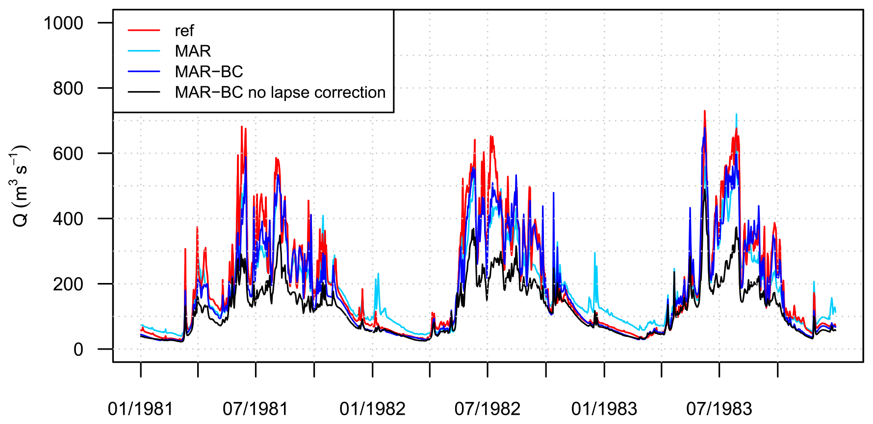
Figure 13Influence on the simulated hydrology of the bias in the temperature lapse rate for the dynamical downscaling model MAR. Illustration with the time series of daily discharges at Rhône@Porte-du-Scex for the 1981–1983 period. ref: simulated discharge from observed weather variables. MAR: simulated discharge from the raw weather scenario. MAR-BC: simulated discharge from the bias-corrected weather scenario considering both the bias correction of the MAT for a given reference elevation and the bias correction of the temperature lapse rate. MAR-BC no lapse correction: simulated discharge from the bias-corrected weather scenario considering only the bias correction of the MAT for a given reference elevation.
The added value of the temperature lapse rate correction for hydrological simulations is thus clearly significant, due to the direct effects of temperature on snow dynamics (snow–rain repartition, snowpack evolution). To the best of our knowledge, the issue of the temperature lapse rate has not received much attention in the past, but it should probably receive more, at least in areas covering large elevation ranges and where highly non-linear behaviours with respect to temperature have to be simulated. These results should also lead scientists to integrate this issue when evaluating dynamical downscaling models and to consider appropriate BC approaches before using model outputs to force impact models.
6.3 Orographic precipitation enhancement
A similar, but different, issue arises for precipitation. As mentioned in Sect. 5.1, significant differences are obtained between MAPs estimated from downscaled simulations and from observations. This translates directly into significant differences in the simulated hydrology. However, the development of relevant MAP estimates is still a challenge in hydro-meteorology, particularly in mountainous areas (e.g. Ruelland, 2020).
In the present study, the MAPs estimated for the reference hydrological simulation are obtained from station observations using Thiessen's weighting method. For the reasons mentioned in the following, no precipitation–elevation relationship was considered in this estimation. However, the annual precipitation generally increases with elevation in the region. This dependency is rather clear from the observations. It is also found in the MAR simulations, although the simulated precipitation lapse rates may overestimate the true ones (Ménégoz et al., 2020a).
The “no precipitation lapse rate” assumption retained for our simulations is therefore not really valid. To illustrate the influence of this assumption, we carried out auxiliary reference simulations using a constant but elevation-dependent adjustment factor for precipitation (e.g. Viviroli et al., 2022). In practice, all precipitation data of a given station are multiplied by a constant value, depending on the difference between the elevation of the station and that of the target hydrological unit, before application of Thiessen's weighting process. Two “with precipitation lapse rate” experiments were performed. The adjustment factors were obtained assuming linear increases of 5 % and 10 % respectively per 100 m of elevation.
As shown in Fig. 14, accounting for a precipitation lapse rate has contrasting effects depending on the area considered. It significantly increases the annual MAP estimates for high-elevation sub-basins (Fig. 14a, left column) but has almost no influence on MAP estimates for low-elevation sub-basins (Fig. 14a, right column). This reflects the under-representation of high-elevation stations in the region. All in all, accounting for a precipitation lapse rate significantly reduces the differences between annual amounts from observations and MAR simulations.
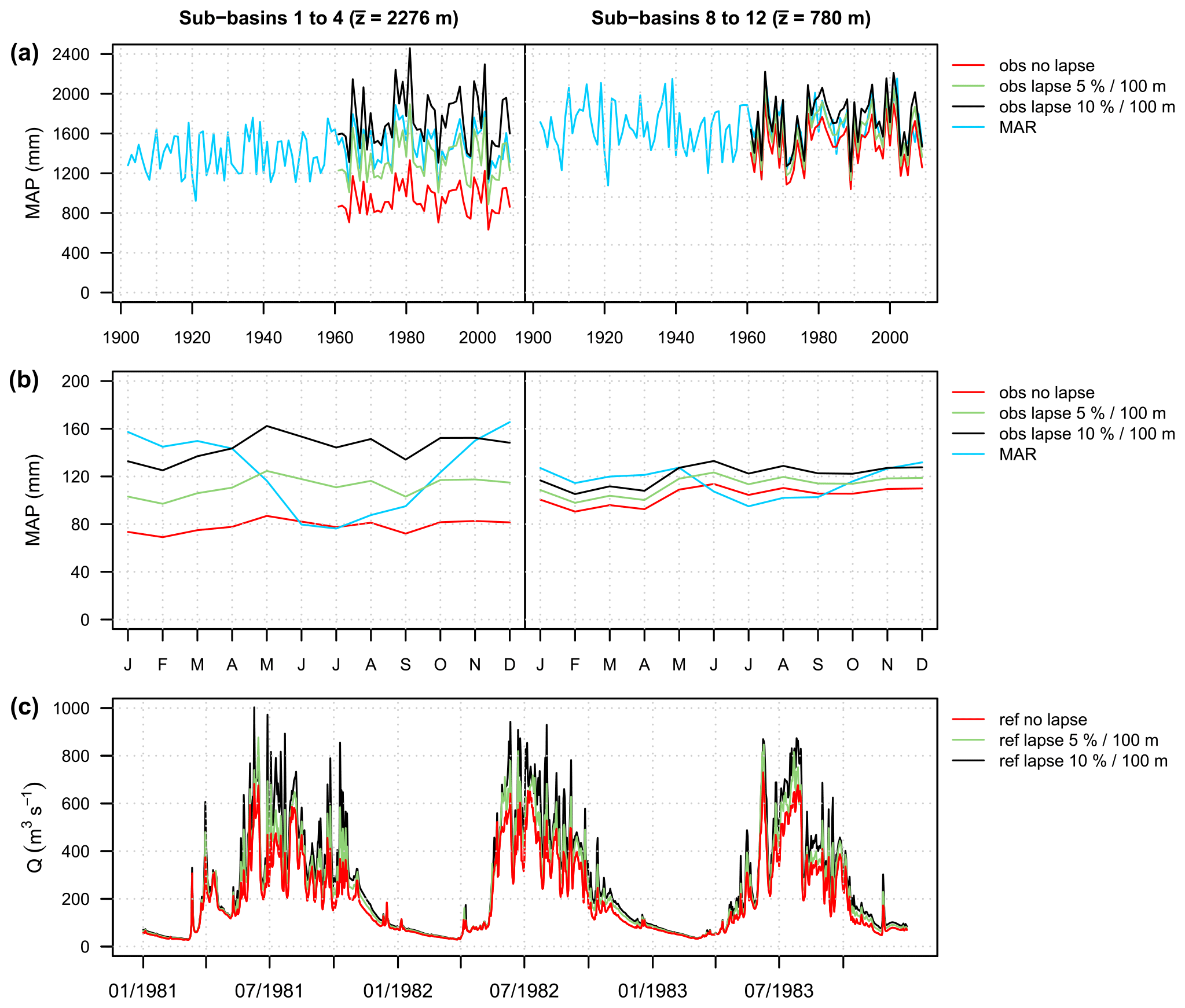
Figure 14(a) Time series of annual MAP (1902–2009) and (b) seasonal cycles of MAP (1961–2009) for two major basins. The average elevation of each major basin is indicated in brackets. obs: observed MAP considering different precipitation lapse rates. MAR: raw MAP scenario produced with the dynamical downscaling model MAR. (c) Time series of daily discharges at Rhône@Porte-du-Scex for the 1981–1983 period. ref: simulated discharge from observed weather variables considering different precipitation lapse rates.
For hydrological simulations, however, the precipitation–elevation dependency is not trivial to take into account in a relevant way. As shown by Ruelland (2020), while the orographic enhancement can be clearly identified from annual and seasonal means, it is no longer evident at the event scale, and for any given event, the spatial pattern of precipitation generally depends on where the precipitation event first occurs. This is likely the reason why the precipitation lapse rate is significantly lower in summer than in winter in the region (Fig. 14b), due to much more frequent convective events (e.g. Ménégoz et al., 2020a). According to Bárdossy and Pegram (2013), on a daily scale, the orographic effects generally contribute a small part to precipitation variations. In many cases, the orographic enhancement obtained for long accumulation durations is often related to more frequent precipitation at high elevations rather than more intense precipitation. Although not verifiable from available observations, this is probably also the case in the region.
Although often determinant, orographic effects cannot be taken into account by a simple and constant adjustment factor, but for practical reasons and lack of better knowledge, this is the usual practice in hydrological modelling. Using a constant adjustment factor for all time steps of a given period is, however, likely to have significant implications for hydrological simulations. This may amplify the highest-precipitation events in an unrealistic way, resulting in turn in huge and unrealistic floods (Hingray et al., 2010). For the URR catchment, hydrological simulations with a precipitation lapse rate produce significantly larger floods (Fig. 14c). With a lapse rate of 5 % per 100 m, the annual daily discharge maxima of the 1961–2009 period increased by 3 % to 106 % (+25 % on average). With a lapse rate of 10 % per 100 m, the increase is even larger (+56 % on average). It is up to 200 % for the largest flood ever observed in the area (15 October 2000) (not shown).
The precipitation–elevation dependency was disregarded in the present work to avoid such unrealistic simulations. This is not really satisfactory, especially regarding the annual water budget of sub-basins. The latter will be misrepresented as a result of the overall dry bias in the precipitation input. Without better knowledge of how precipitation amounts depend on elevation at the event scale, disregarding the elevation dependency was found to be an acceptable compromise option if relevant flood events have to be simulated.
Note that, in our simulations, the dry bias is probably compensated for during hydrological parameter optimisation. Parameter optimisation generally has the effect of forcing the model to close the water balance. Reservoir-based conceptual models, such as the one used here, can thus compensate for missing precipitation by reducing the evapotranspiration losses. This problem is well known but rarely discussed. An example is the work of Minville et al. (2014).
6.4 The hydrological model: a powerful assessment tool despite its limitations
In this work, we assessed and compared the ability of two downscaling models to simulate hydrologically relevant weather scenarios. The hydrological model considered here for this assessment is obviously not free of limitations.
In the model, as mentioned in the previous section, the influence of orography on precipitation was disregarded to avoid the generation of irrelevant floods. This representation is obviously far from satisfactory, and more relevant representations, at the event scale especially, would be worth considering in future years when available.
The mean areal precipitation and temperature were estimated for each spatial unit of the model using Thiessen's weighting method. This is a rather crude method, and other methods may provide better estimates (e.g. inverse distance weighting or kriging with external drift; Wagner et al., 2012). However, they also have important limitations in mountainous environments (e.g. difficulty in accounting for the influence of topography on weather spatial patterns at the event scale). Thiessen's weighting method was retained here for its simplicity and its ability to take into account the time-varying temperature–elevation relationship in a straightforward way.
The hydrological model also relies on assumptions that are potentially crude. For instance, the characteristics of the sub-basins are assumed not to have changed over the last century. For the glacier cover, this assumption does not really hold. According to Huss (2011), however, the contribution of glacier melt in the region was relatively stable over the 20th century, with a similar glacier contribution during the periods 1961–1990 and 1908–2008. The glacier retreat strengthened over the period 1988–2008, but the corresponding increase in the glacier contribution to the URR discharges was found to be rather limited (13 % in August). While not fully satisfactory, the assumption of a constant glacier therefore seems reasonable.
The signature-based calibration of the model, used for sub-basins with altered discharge data, is also not optimal. The objective function considered for the calibration, for instance, gives considerable weight to the statistical distribution of annual daily discharge maxima. Other results may be obtained by adding criteria for low flows (e.g. a distribution of annual monthly discharge minima). This will be worth further investigations. On the other hand, parameters were calibrated so that simulated signatures reproduce at best observed ones, but observed and simulated signatures come from different periods. We thus implicitly assume that the weather regimes and the natural hydrological behaviour of the URR sub-basins have not changed significantly over the last century. Both assumptions seem to be reasonable to a first approximation. Indeed, over the last century, no significant trends in precipitation have been observed in the region (Masson and Frei, 2016), and the hydrological regimes of the natural sub-basins have remained almost unchanged (see Fig. S9).
The hydrological model is thus not optimal for a number of reasons. However, this is not expected to influence the main results of our study. Indeed, the model is mainly used here as a complex and non-linear filter to assess the ability of the downscaling chains to simulate hydrologically relevant weather scenarios. In this impact-oriented assessment context, the hydrological model can be imperfect, as it can also be used to produce the hydrological reference against which the hydrological scenarios will be compared. In the context of the URR catchment, the model is a powerful tool for achieving an impact-oriented assessment of downscaled weather scenarios in contrasting and demanding hydro-meteorological configurations, where the interplay between weather variables, in both space and time, is determinant.
In this study, two hydro-meteorological modelling chains were used to simulate the past variations in discharge at several stations of the upper Rhône River catchment, a mesoscale catchment in the western Alps. The discharges were simulated with the glacio-hydrological GSM-SOCONT model using weather scenarios downscaled with the MAR and SCAMP models from the data of the global atmospheric reanalysis ERA-20C. MAR is a dynamical downscaling model, SCAMP a statistical one providing an ensemble of downscaled scenarios.
The originality of this study is fourfold. (i) We evaluated the modelling chains in contrasting and demanding hydro-meteorological configurations where the interplay between weather variables, in both space and time, is determinant. (ii) The spatio-temporal relevance of the weather scenarios is assessed by their hydrological responses, simulated using an ad hoc hydrological model at several gauging stations. (iii) The simulations cover the entire 20th century, a period long enough to assess the ability of the modelling chains to reproduce daily variations in observed discharges, low-frequency events and variations in low-flow and flood activities. (iv) For both downscaling models, we evaluated the need for additional bias correction of the weather scenarios, including that of temperature lapse rates.
This framework allowed us to highlight important criteria to be met for the simulation of relevant hydrological scenarios for the upper Rhône River catchment. The alpine configuration of the upper Rhône River catchment (unknown effects of the large upstream dams and of the regulation of Lake Geneva, scarcity of concomitant weather and discharge observations) made the calibration of the hydrological model rather difficult. This required the development of an original multiple-calibration strategy based on both observed discharge time series and hydrological signatures.
For both modelling chains, given this difficult modelling context and the fact that the weather scenarios are only produced from large-scale atmospheric information, the simulated discharges are globally in good agreement with the reference ones. For the 1961–2009 period, the multi-scale variations in reference discharges (daily, seasonal and interannual) are reproduced well. To some extent, the simulations also reproduce the annual monthly discharge minima and the annual daily discharge maxima quite well. For the first half of the century, the agreement with the reference discharges is lower (but still reasonable), likely due to lower data quality (ERA-20C and discharge data) and/or some modelling assumptions and choices (e.g. signature-based calibration, stationarity assumption). Nevertheless, both modelling chains are able to accurately reproduce the variations in flood activity over the last century. The results for low-flow activity are less satisfactory.
Both modelling chains are likely to be appropriate for the generation of relevant regional weather scenarios for different climate contexts from outputs of ad hoc GCM experiments. Thanks to its much lower computational cost, the SCAMP model is to be favoured when large ensembles of climate simulations have to be downscaled. The statistical nature of SCAMP also allows us to account for the uncertainty in the downscaling relationship. The ensemble of weather scenarios generated by SCAMP for any large-scale scenario thus allows us to simulate and account for the small-scale internal variability of weather. This is another advantage over MAR, allowing a more robust assessment of possible low-frequency changes in hydro-meteorological regimes (e.g. Lafaysse et al., 2014). In a future study, we will force the SCAMP–GSM-SOCONT chain with a CMIP6–PMIP4 palaeo-simulation ensemble (Jungclaus et al., 2017; Kageyama et al., 2018) to assess the variations in hydro-meteorological regimes of the upper Rhône River catchment over the last millennium. We also expect to confront the simulated variations in flood activity with those obtained in previous works from the sediment archives of Lake Bourget (Jenny et al., 2014; Evin et al., 2019; Wilhelm et al., 2022). Moreover, this could also corroborate the influence of warming and atmospheric circulation changes on multi-decadal flood activity over the last 2 centuries, recently highlighted by Brönnimann et al. (2022) for different European rivers.
As already shown in previous works, the hydrological behaviour of river basins can be simulated from large-scale atmospheric information only. In this study, we also showed that the simulation of hydrologically relevant weather scenarios required a bias correction of the downscaled weather scenarios. The highly non-linear behaviour of hydrological systems does not bear biased weather. This was made evident here for temperature, due to the highly non-linear thermal sensitivity of snow variables. If it seeks to be relevant, the bias correction step is not necessarily straightforward (Maraun, 2016; Switanek et al., 2022). For temperature, the bias correction is commonly applied for the temperatures of reference stations. For the upper Rhône River catchment, the bias correction was also needed for the temperature lapse rate simulated by the dynamical downscaling model MAR. The temperature lapse rate correction was determinant to avoid irrelevant simulations of the snowpack dynamics at high elevations and consequently of the hydrology.
The bias correction was also required for precipitation. Significant differences were also found between the reference and downscaled precipitation, particularly for MAR in winter. The bias correction of downscaled precipitation was thus also applied so that the statistical distribution of precipitation scenarios fits that of the reference. However, the quality of the reference is questionable. It was indeed developed by disregarding the significant precipitation–elevation relationship in the area to avoid the simulation of irrelevant flood events. The much larger precipitation amounts simulated by MAR for high-elevation sub-basins are thus not necessarily irrelevant considering the snowfall undercatch issues (Kochendorfer et al., 2017). An interesting perspective of this work would be to recalibrate the hydrological model using MAR data that provide these larger precipitation amounts at high elevations, to study their physical realism. Overall, a better understanding of the precipitation–elevation relationship in mountainous areas, especially its likely variations in time and its dependency on event types, would improve hydro-meteorological analyses and simulations and make them more relevant. This would benefit from more observations in high-altitude areas, a critical issue pointed out for a long time (e.g. Hingray et al., 2012). Despite their multiple limitations in mountainous areas, radar data could also provide valuable insights into orographic drivers of precipitation (e.g. Germann et al., 2022).
If downscaling models clearly need to be refined in the future, scientists should also consider improving the bias correction methods for such challenging configurations. They should also consider the possibility of better understanding and accounting for the precipitation orographic enhancement at the event scale. Dynamical downscaling models such as MAR are likely promising tools for such analyses, but their value for areas with marked relief should be better estimated.
MAR is accessible at https://gitlab.com/Mar-Group (GitLab, 2024). SCAMP is available upon request. GSM-SOCONT is accessible at https://fr.mathworks.com/matlabcentral/fileexchange/43452-gsm-socont-glacio-hydrological-model (GSM-SOCONT, 2024).
The outputs of the MAR experiment used in this study can be downloaded at https://doi.org/10.5281/zenodo.3674607 (Ménégoz et al., 2020b). The meteorological and hydrological simulation data from the four modelling chains are available upon request.
The supplement related to this article is available online at: https://doi.org/10.5194/hess-28-2139-2024-supplement.
This study is part of CL's PhD thesis. BW and BH supervised the PhD. All the authors contributed to the design of the study and the analysis framework. CL performed the simulations and produced the figures presented in this study. CL, MM and BH contributed to the writing of the document and to the editing of the paper.
The contact author has declared that none of the authors has any competing interests.
Publisher's note: Copernicus Publications remains neutral with regard to jurisdictional claims made in the text, published maps, institutional affiliations, or any other geographical representation in this paper. While Copernicus Publications makes every effort to include appropriate place names, the final responsibility lies with the authors.
A part of the simulations was performed with the Grenoble Alpes Research Data and Computing Infrastructure (GRICAD; https://gricad.univ-grenoble-alpes.fr/, last access: 14 May 2024). We would like to thank Mondher Chekki for his valuable technical and informatics support as well as Julien Beaumet for providing the outputs of the MAR simulation. We also thank the editor and four reviewers for their constructive comments, which helped us to improve the manuscript.
This research has been supported by the French National Research Agency in the framework of the Investissements d'avenir programme (ANR-15-IDEX-02).
This paper was edited by Adriaan J. (Ryan) Teuling and reviewed by Juraj Parajka and three anonymous referees.
Arnell, N. W., Hudson, D. A., and Jones, R. G.: Climate change scenarios from a regional climate model: Estimating change in runoff in southern Africa, J. Geophys. Res., 108, 4519, https://doi.org/10.1029/2002JD002782, 2003. a
Bárdossy, A.: Calibration of hydrological model parameters for ungauged catchments, Hydrol. Earth Syst. Sci., 11, 703–710, https://doi.org/10.5194/hess-11-703-2007, 2007. a
Bárdossy, A. and Pegram, G.: Interpolation of precipitation under topographic influence at different time scales: Interpolation of Precipitation, Water Resour. Res., 49, 4545–4565, https://doi.org/10.1002/wrcr.20307, 2013. a
Beaumet, J., Ménégoz, M., Morin, S., Gallée, H., Fettweis, X., Six, D., Vincent, C., Wilhelm, B., and Anquetin, S.: Twentieth century temperature and snow cover changes in the French Alps, Reg. Environ. Change, 21, 114, https://doi.org/10.1007/s10113-021-01830-x, 2021. a
Bechtold, P., Bazile, E., Guichard, F., Mascart, P., and Richard, E.: A mass-flux convection scheme for regional and global models, Q. J. Roy. Meteorol. Soc., 127, 869–886, https://doi.org/10.1002/qj.49712757309, 2001. a
Beniston, M.: Mountain Weather and Climate: A General Overview and a Focus on Climatic Change in the Alps, Hydrobiologia, 562, 3–16, https://doi.org/10.1007/s10750-005-1802-0, 2006. a
Blöschl, G., Hall, J., Parajka, J., Perdigão, R. A. P., Merz, B., Arheimer, B., Aronica, G. T., Bilibashi, A., Bonacci, O., Borga, M., Čanjevac, I., Castellarin, A., Chirico, G. B., Claps, P., Fiala, K., Frolova, N., Gorbachova, L., Gül, A., Hannaford, J., Harrigan, S., Kireeva, M., Kiss, A., Kjeldsen, T. R., Kohnová, S., Koskela, J. J., Ledvinka, O., Macdonald, N., Mavrova-Guirguinova, M., Mediero, L., Merz, R., Molnar, P., Montanari, A., Murphy, C., Osuch, M., Ovcharuk, V., Radevski, I., Rogger, M., Salinas, J. L., Sauquet, E., Šraj, M., Szolgay, J., Viglione, A., Volpi, E., Wilson, D., Zaimi, K., and Živković, N.: Changing climate shifts timing of European floods, Science, 357, 588–590, https://doi.org/10.1126/science.aan2506, 2017. a
Boé, J., Terray, L., Habets, F., and Martin, E.: Statistical and dynamical downscaling of the Seine basin climate for hydro-meteorological studies, Int. J. Climatol., 27, 1643–1655, https://doi.org/10.1002/joc.1602, 2007. a, b
Bonnet, R., Boé, J., Dayon, G., and Martin, E.: Twentieth‐Century Hydrometeorological Reconstructions to Study the Multidecadal Variations of the Water Cycle Over France, Water Resour. Res., 53, 8366–8382, https://doi.org/10.1002/2017WR020596, 2017. a, b
Bonnet, R., Boé, J., and Habets, F.: Influence of multidecadal variability on high and low flows: the case of the Seine basin, Hydrol. Earth Syst. Sci., 24, 1611–1631, https://doi.org/10.5194/hess-24-1611-2020, 2020. a
Brönnimann, S., Stucki, P., Franke, J., Valler, V., Brugnara, Y., Hand, R., Slivinski, L. C., Compo, G. P., Sardeshmukh, P. D., Lang, M., and Schaefli, B.: Influence of warming and atmospheric circulation changes on multidecadal European flood variability, Clim. Past, 18, 919–933, https://doi.org/10.5194/cp-18-919-2022, 2022. a
Brun, E., David, P., Sudul, M., and Brunot, G.: A numerical model to simulate snow-cover stratigraphy for operational avalanche forecasting, J. Glaciol., 38, 13–22, https://doi.org/10.3189/S0022143000009552, 1992. a
Caillouet, L., Vidal, J.-P., Sauquet, E., Devers, A., and Graff, B.: Ensemble reconstruction of spatio-temporal extreme low-flow events in France since 1871, Hydrol. Earth Syst. Sci., 21, 2923–2951, https://doi.org/10.5194/hess-21-2923-2017, 2017. a
CERCG: Règlement sur la manoeuvre de l'ouvrage de régularisation du niveau du lac Léman à Genève, Arrêté du 17 septembre 1997, Genève, Suisse, https://www.lexfind.ch/tolv/190761/fr (last access: 14 May 2024), 1997. a
Chagnaud, G., Gallée, H., Lebel, T., Panthou, G., and Vischel, T.: A Boundary Forcing Sensitivity Analysis of the West African Monsoon Simulated by the Modèle Atmosphérique Régional, Atmosphere, 11, 191, https://doi.org/10.3390/atmos11020191, 2020. a
Chardon, J., Hingray, B., Favre, A.-C., Autin, P., Gailhard, J., Zin, I., and Obled, C.: Spatial Similarity and Transferability of Analog Dates for Precipitation Downscaling over France, J. Climate, 27, 5056–5074, https://doi.org/10.1175/JCLI-D-13-00464.1, 2014. a, b
Chardon, J., Favre, A.-C., and Hingray, B.: Effects of Spatial Aggregation on the Accuracy of Statistically Downscaled Precipitation Predictions, J. Hydrometeorol., 17, 1561–1578, https://doi.org/10.1175/JHM-D-15-0031.1, 2016. a
Chardon, J., Hingray, B., and Favre, A.-C.: An adaptive two-stage analog/regression model for probabilistic prediction of small-scale precipitation in France, Hydrol. Earth Syst. Sci., 22, 265–286, https://doi.org/10.5194/hess-22-265-2018, 2018. a
Clark, M., Gangopadhyay, S., Hay, L., Rajagopalan, B., and Wilby, R.: The Schaake Shuffle: A Method for Reconstructing Space-Time Variability in Forecasted Precipitation and Temperature Fields, J. Hydrometeorol., 5, 243–262, https://doi.org/10.1175/1525-7541(2004)005<0243:TSSAMF>2.0.CO;2, 2004. a
Dayon, G., Boe, J., and Martin, E.: Transferability in the future climate of a statistical downscaling method for precipitation in France, J. Geophys. Res.-Atmos., 120, 1023–1043, https://doi.org/10.1002/2014JD022236, 2015. a
Déqué, M.: Frequency of precipitation and temperature extremes over France in an anthropogenic scenario: Model results and statistical correction according to observed values, Global Planet. Change, 57, 16–26, https://doi.org/10.1016/j.gloplacha.2006.11.030, 2007. a
De Ridder, K. and Schayes, G.: The IAGL Land Surface Model, J. Appl. Meteorol., 36, 167–182, https://doi.org/10.1175/1520-0450(1997)036<0167:TILSM>2.0.CO;2, 1997. a
Devers, A., Vidal, J.-P., Lauvernet, C., and Vannier, O.: FYRE Climate: A high-resolution reanalysis of daily precipitation and temperature in France from 1871 to 2012, Clim. Past, 17, 1857–1879, https://doi.org/10.5194/cp-17-1857-2021, 2021. a
Di Sante, F., Coppola, E., and Giorgi, F.: Projections of river floods in Europe using EURO-CORDEX, CMIP5 and CMIP6 simulations, Int. J. Climatol., 41, 3203–3221, https://doi.org/10.1002/joc.7014, 2021. a
Doutreloup, S., Wyard, C., Amory, C., Kittel, C., Erpicum, M., and Fettweis, X.: Sensitivity to Convective Schemes on Precipitation Simulated by the Regional Climate Model MAR over Belgium (1987–2017), Atmosphere, 10, 34, https://doi.org/10.3390/atmos10010034, 2019. a
Evin, G., Wilhelm, B., and Jenny, J.-P.: Flood hazard assessment of the Rhône River revisited with reconstructed discharges from lake sediments, Global Planet. Change, 172, 114–123, https://doi.org/10.1016/j.gloplacha.2018.09.010, 2019. a
Evin, G., Somot, S., and Hingray, B.: Balanced estimate and uncertainty assessment of European climate change using the large EURO-CORDEX regional climate model ensemble, Earth Syst. Dynam., 12, 1543–1569, https://doi.org/10.5194/esd-12-1543-2021, 2021. a
Fowler, H. J., Blenkinsop, S., and Tebaldi, C.: Linking climate change modelling to impacts studies: recent advances in downscaling techniques for hydrological modelling, Int. J. Climatol., 27, 1547–1578, https://doi.org/10.1002/joc.1556, 2007. a
Froidurot, S., Zin, I., Hingray, B., and Gautheron, A.: Sensitivity of Precipitation Phase over the Swiss Alps to Different Meteorological Variables, J. Hydrometeorol., 15, 685–696, https://doi.org/10.1175/JHM-D-13-073.1, 2014. a
Gallée, H.: Simulation of the Mesocyclonic Activity in the Ross Sea, Antarctica, Mon. Weather Rev., 123, 2051–2069, https://doi.org/10.1175/1520-0493(1995)123<2051:SOTMAI>2.0.CO;2, 1995. a
Gallée, H. and Duynkerke, P. G.: Air-snow interactions and the surface energy and mass balance over the melting zone of west Greenland during the Greenland Ice Margin Experiment, J. Geophys. Res.-Atmos., 102, 13813–13824, https://doi.org/10.1029/96JD03358, 1997. a
Gallée, H. and Schayes, G.: Development of a 3-Dimensional Meso-Gamma Primitive Equation Model – Katabatic Winds Simulation in the Area of Terra-Nova Bay, Antarctica, Mon. Weather Rev., 122, 671–685, https://doi.org/10.1175/1520-0493(1994)122<0671:DOATDM>2.0.CO;2, 1994. a, b
Gallée, H., Pettré, P., and Schayes, G.: Sudden Cessation of Katabatic Winds in Adélie Land, Antarctica, J. Appl. Meteorol., 35, 1142–1152, https://doi.org/10.1175/1520-0450(1996)035<1142:SCOKWI>2.0.CO;2, 1996. a, b
Gallée, H., Guyomarc'h, G., and Brun, E.: Impact Of Snow Drift On The Antarctic Ice Sheet Surface Mass Balance: Possible Sensitivity To Snow-Surface Properties, Bound.-Lay. Meteorol., 99, 1–19, https://doi.org/10.1023/A:1018776422809, 2001. a
Gangopadhyay, S., Clark, M., and Rajagopalan, B.: Statistical downscaling using K-nearest neighbors, Water Resour. Res., 41, W02024, https://doi.org/10.1029/2004WR003444, 2005. a
Germann, U., Boscacci, M., Clementi, L., Gabella, M., Hering, A., Sartori, M., Sideris, I. V., and Calpini, B.: Weather Radar in Complex Orography, Remote Sens., 14, 503, https://doi.org/10.3390/rs14030503, 2022. a
Giorgi, F. and Mearns, L. O.: Approaches to the simulation of regional climate change: A review, Rev. Geophys., 29, 191–216, https://doi.org/10.1029/90RG02636, 1991. a
GitLab: Atmospheric Regional Model, https://gitlab.com/Mar-Group (last access: 14 May 2024), 2024. a
GLIMS: Glacier Database, Boulder Colorado, USA, NASA, National Snow and Ice Data Center [data set], https://doi.org/10.7265/N5V98602, 2015. a, b
Grandjean, P.: La régularisation du lac Léman, Hydrology in Mountainous Regions, I – Hydrological Measurements: the Water Cycle, Proceedings of two Lausanne Symposia, IAHS, 193, 769–776, 1990. a
GSM-SOCONT: Glacio-hydrological model, https://fr.mathworks.com/matlabcentral/fileexchange/43452-gsm-socont-glacio-hydrological-model (last access: 14 May 2024), 2024. a
Hanssen-Bauer, I., Achberger, C., Benestad, R. E., Chen, D., and Førland, E. J.: Statistical downscaling of climate scenarios over Scandinavia, Clim. Res., 29, 255–268, https://doi.org/10.3354/cr029255, 2005. a
Harris, I., Jones, P., Osborn, T., and Lister, D.: Updated high-resolution grids of monthly climatic observations – the CRU TS3.10 Dataset, Int. J. Climatol., 34, 623–642, https://doi.org/10.1002/joc.3711, 2014. a
Hersbach, H., Bell, B., Berrisford, P., Hirahara, S., Horányi, A., Muñoz‐Sabater, J., Nicolas, J., Peubey, C., Radu, R., Schepers, D., Simmons, A., Soci, C., Abdalla, S., Abellan, X., Balsamo, G., Bechtold, P., Biavati, G., Bidlot, J., Bonavita, M., Chiara, G., Dahlgren, P., Dee, D., Diamantakis, M., Dragani, R., Flemming, J., Forbes, R., Fuentes, M., Geer, A., Haimberger, L., Healy, S., Hogan, R. J., Hólm, E., Janisková, M., Keeley, S., Laloyaux, P., Lopez, P., Lupu, C., Radnoti, G., Rosnay, P., Rozum, I., Vamborg, F., Villaume, S., and Thépaut, J.: The ERA5 global reanalysis, Q. J. Roy. Meteorol. Soc., 146, 1999–2049, https://doi.org/10.1002/qj.3803, 2020. a
Hingray, B., Schaefli, B., Mezghani, A., and Hamdi, Y.: Signature-based model calibration for hydrological prediction in mesoscale Alpine catchments, Hydrolog. Sci. J., 55, 1002–1016, https://doi.org/10.1080/02626667.2010.505572, 2010. a, b, c, d, e
Hingray, B., Dedieu, J.-P., Lebel, T., Obled, C., Sicart, J.-E., Six, D., Vincent, C., Wagnon, P., and Zin, I.: Observations glaciologiques et hydrométéorologiques en zone de montagne: quelques problématiques et perspectives actuelles, La Houille Blanche, 2, 5–11, https://doi.org/10.1051/lhb/2012009, 2012. a
Hingray, B., Picouet, C., and Musy, A.: Hydrology A Science for Engineers, CRC Press, 592 pp., ISBN 9781466590595, 2014. a, b
Horton, P. and Brönnimann, S.: Impact of global atmospheric reanalyses on statistical precipitation downscaling, Clim. Dynam., 52, 5189–5211, https://doi.org/10.1007/s00382-018-4442-6, 2019. a
Huss, M.: Present and future contribution of glacier storage change to runoff from macroscale drainage basins in Europe, Water Resour. Res., 47, W07511, https://doi.org/10.1029/2010WR010299, 2011. a
Isotta, F. A., Frei, C., Weilguni, V., Tadic, M. P., Lassegues, P., Rudolf, B., Pavan, V., Cacciamani, C., Antolini, G., Ratto, S. M., Munari, M., Micheletti, S., Bonati, V., Lussana, C., Ronchi, C., Panettieri, E., Marigo, G., and Vertacnik, G.: The climate of daily precipitation in the Alps: development and analysis of a high-resolution grid dataset from pan-Alpine rain-gauge data, Int. J. Climatol., 34, 1657–1675, https://doi.org/10.1002/joc.3794, 2014. a
Jenny, J.-P., Wilhelm, B., Arnaud, F., Sabatier, P., Giguet Covex, C., Mélo, A., Fanget, B., Malet, E., Ployon, E., and Perga, M. E.: A 4D sedimentological approach to reconstructing the flood frequency and intensity of the Rhône River (Lake Bourget, NW European Alps), J. Paleolimnol., 51, 469–483, https://doi.org/10.1007/s10933-014-9768-4, 2014. a
Jungclaus, J. H., Bard, E., Baroni, M., Braconnot, P., Cao, J., Chini, L P., Egorova, T., Evans, M., González-Rouco, J. F., Goosse, H., Hurtt, G. C., Joos, F., Kaplan, J. O., Khodri, M., Klein Goldewijk, K., Krivova, N., LeGrande, A. N., Lorenz, S. J., Luterbacher, J., Man, W., Maycock, A. C., Meinshausen, M., Moberg, A., Muscheler, R., Nehrbass-Ahles, C., Otto-Bliesner, B. I., Phipps, S. ., Pongratz, J., Rozanov, E., Schmidt, G. A., Schmidt, H., Schmutz, W., Schurer, A., Shapiro, A. I., Sigl, M., Smerdon, J. E., Solanki, S. K., Timmreck, C., Toohey, M., Usoskin, I. G., Wagner, S., Wu, C.-J., Yeo, K. L., Zanchettin, D., Zhang, Q., and Zorita, E.: The PMIP contribution to CMIP6 – Part 3: The last millennium, scientific objective, and experimental design for the PMIP4 past1000 simulations, Geosci. Model Dev., 10, 4005–4033, https://doi.org/10.5194/gmd-10-4005-2017, 2017. a
Kageyama, M., Braconnot, P., Harrison, S. P., Haywood, A. M., Jungclaus, J. H., Otto-Bliesner, B. L., Peterschmitt, J.-Y., Abe-Ouchi, A., Albani, S., Bartlein, P. J., Brierley, C., Crucifix, M., Dolan, A., Fernandez-Donado, L., Fischer, H., Hopcroft, P. O., Ivanovic, R. F., Lambert, F., Lunt, D. J., Mahowald, N. M., Peltier, W. R., Phipps, S. J., Roche, D. M., Schmidt, G. A., Tarasov, L., Valdes, P. J., Zhang, Q., and Zhou, T.: The PMIP4 contribution to CMIP6 – Part 1: Overview and over-arching analysis plan, Geosci. Model Dev., 11, 1033–1057, https://doi.org/10.5194/gmd-11-1033-2018, 2018. a
Kochendorfer, J., Rasmussen, R., Wolff, M., Baker, B., Hall, M. E., Meyers, T., Landolt, S., Jachcik, A., Isaksen, K., Brækkan, R., and Leeper, R.: The quantification and correction of wind-induced precipitation measurement errors, Hydrol. Earth Syst. Sci., 21, 1973–1989, https://doi.org/10.5194/hess-21-1973-2017, 2017. a
Kuchment, L. and Gelfan, A.: The determination of the snowmelt rate and the meltwater outflow from a snowpack for modelling river runoff generation, J. Hydrol., 179, 23–36, https://doi.org/10.1016/0022-1694(95)02878-1, 1996. a
Kuentz, A., Mathevet, T., Gailhard, J., and Hingray, B.: Building long-term and high spatio-temporal resolution precipitation and air temperature reanalyses by mixing local observations and global atmospheric reanalyses: the ANATEM model, Hydrol. Earth Syst. Sci., 19, 2717–2736, https://doi.org/10.5194/hess-19-2717-2015, 2015. a, b, c
Kundzewicz, Z. W., Krysanova, V., Dankers, R., Hirabayashi, Y., Kanae, S., Hattermann, F. F., Huang, S., Milly, P. C. D., Stoffel, M., Driessen, P. P. J., Matczak, P., Quevauviller, P., and Schellnhuber, H.-J.: Differences in flood hazard projections in Europe – their causes and consequences for decision making, Hydrolog. Sci. J., 62, 1–14, https://doi.org/10.1080/02626667.2016.1241398, 2016. a
Lafaysse, M., Hingray, B., Mezghani, A., Gailhard, J., and Terray, L.: Internal variability and model uncertainty components in future hydrometeorological projections: The Alpine Durance basin, Water Resour. Res., 50, 3317–3341, https://doi.org/10.1002/2013WR014897, 2014. a, b, c, d
Leander, R., Buishand, T. A., van den Hurk, B. J. J. M., and de Wit, M. J. M.: Estimated changes in flood quantiles of the river Meuse from resampling of regional climate model output, J. Hydrol., 351, 331–343, https://doi.org/10.1016/j.jhydrol.2007.12.020, 2008. a
Lemaitre-Basset, T., Collet, L., Thirel, G., Parajka, J., Evin, G., and Hingray, B.: Climate change impact and uncertainty analysis on hydrological extremes in a French Mediterranean catchment, Hydrolog. Sci. J., 66, 888–903, https://doi.org/10.1080/02626667.2021.1895437, 2021. a
Leung, L. R. and Qian, Y.: Atmospheric rivers induced heavy precipitation and flooding in the western US simulated by the WRF regional climate model, Geophys. Res. Lett., 36, L03820, https://doi.org/10.1029/2008GL036445, 2009. a
Lorenz, E. N.: Atmospheric Predictability as Revealed by Naturally Occurring Analogues, J. Atmos. Sci., 26, 636–646, https://doi.org/10.1175/1520-0469(1969)26<636:APARBN>2.0.CO;2, 1969. a
Maraun, D.: Bias Correcting Climate Change Simulations – a Critical Review, Curr. Clim. Change Rep., 2, 211–220, https://doi.org/10.1007/s40641-016-0050-x, 2016. a
Maraun, D., Wetterhall, F., Ireson, A. M., Chandler, R. E., Kendon, E. J., Widmann, M., Brienen, S., Rust, H. W., Sauter, T., Themeßl, M., Venema, V. K. C., Chun, K. P., Goodess, C. M., Jones, R. G., Onof, C., Vrac, M., and Thiele-Eich, I.: Precipitation downscaling under climate change: Recent developments to bridge the gap between dynamical models and the end user, Rev. Geophys., 48, RG3003, https://doi.org/10.1029/2009RG000314, 2010. a
Marty, R., Zin, I., Obled, C., Bontron, G., and Djerboua, A.: Toward Real-Time Daily PQPF by an Analog Sorting Approach: Application to Flash-Flood Catchments, J. Appl. Meteorol. Clim., 51, 505–520, https://doi.org/10.1175/JAMC-D-11-011.1, 2012. a
Masson, D. and Frei, C.: Long-term variations and trends of mesoscale precipitation in the Alps: recalculation and update for 1901–2008, Int. J. Climatol., 36, 492–500, https://doi.org/10.1002/joc.4343, 2016. a
Masson-Delmotte, V., Zhai, P., Pirani, A., Connors, S. L., Péan, C., Berger, S., Caud, N., Chen, Y., Goldfarb, L., Gomis, M. I., Huang, M., Leitzell, K., Lonnoy, E., Matthews, J. B. R., Maycock, T. K., Waterfield, T., Yelekçi, O., Yu, R., and Zhou, B.: Climate Change 2021: The Physical Science Basis, in: Contribution of Working Group I to the Sixth Assessment Report of the Intergovernmental Panel on Climate Change, Cambridge University Press, Cambridge, UK and New York, NY, USA, 2391 pp., https://doi.org/10.1017/9781009157896, 2021. a
Ménégoz, M., Gallée, H., and Jacobi, H. W.: Precipitation and snow cover in the Himalaya: from reanalysis to regional climate simulations, Hydrol. Earth Syst. Sci., 17, 3921–3936, https://doi.org/10.5194/hess-17-3921-2013, 2013. a
Ménégoz, M., Valla, E., Jourdain, N. C., Blanchet, J., Beaumet, J., Wilhelm, B., Gallée, H., Fettweis, X., Morin, S., and Anquetin, S.: Contrasting seasonal changes in total and intense precipitation in the European Alps from 1903 to 2010, Hydrol. Earth Syst. Sci., 24, 5355–5377, https://doi.org/10.5194/hess-24-5355-2020, 2020a. a, b, c
Ménégoz, M., Fettweis, X., Gallée, H., Belleflamme, A., and Beaumet, J.: Climate simulation over the European Alps for the period 1902–2010 produced with the model MAR, MAR_Alps_v0, Zenodo [data set], https://doi.org/10.5281/zenodo.3674607, 2020b. a
Metzger, A.: Retour d'est – La géochronique du temps qu'il fait, La Géographie, 1588, 64–65, https://doi.org/10.3917/geo.1588.0064, 2023. a
Mezghani, A. and Hingray, B.: A combined downscaling-disaggregation weather generator for stochastic generation of multisite hourly weather variables over complex terrain: Development and multi-scale validation for the Upper Rhone River basin, J. Hydrol., 377, 245–260, https://doi.org/10.1016/j.jhydrol.2009.08.033, 2009. a
Minville, M., Cartier, D., Guay, C., Leclaire, L., Audet, C., Le Digabel, S., and Merleau, J.: Improving process representation in conceptual hydrological model calibration using climate simulations, Water Resour. Res., 50, 5044–5073, https://doi.org/10.1002/2013WR013857, 2014. a
Nabat, P., Somot, S., Mallet, M., Sanchez‐Lorenzo, A., and Wild, M.: Contribution of anthropogenic sulfate aerosols to the changing Euro‐Mediterranean climate since 1980, Geophys. Res. Lett., 41, 5605–5611, https://doi.org/10.1002/2014GL060798, 2014. a
Nash, J. and Sutcliffe, J.: River flow forecasting through conceptual models part I – A discussion of principles, J. Hydrol., 10, 282–290, https://doi.org/10.1016/0022-1694(70)90255-6, 1970. a
Obled, C., Bontron, G., and Garçon, R.: Quantitative precipitation forecasts: a statistical adaptation of model outputs through an analogues sorting approach, Atmos. Res., 63, 303–324, https://doi.org/10.1016/S0169-8095(02)00038-8, 2002. a, b
Obled, C., Zin, I., and Hingray, B.: Choix des pas de temps et d'espace pour des modélisations parcimonieuses en hydrologie des crues, La Houille Blanche, 5, 81–87, https://doi.org/10.1051/lhb/2009059, 2009. a
OFEG: Les crues 2000 – Analyse des événements/cas exemplaires, Rapports de l'OFEG, Série Eaux, 2, no. BWGW-2-F, Office fédéral de l'environnement OFEV, Berne, Suisse, 248 pp., https://www.bafu.admin.ch/bafu/fr/home/themes/dangers-naturels/publications-etudes/publications/les-crues-2000-analyse-des-evenements-cas-exemplaires.html (last access: 14 May 2024), 2002. a
Poli, P., Hersbach, H., Dee, D. P., Berrisford, P., Simmons, A. J., Vitart, F., Laloyaux, P., Tan, D. G. H., Peubey, C., Thépaut, J.-N., Trémolet, Y., Hólm, E. V., Bonavita, M., Isaksen, L., and Fisher, M.: ERA-20C: An Atmospheric Reanalysis of the Twentieth Century, J. Climate, 29, 4083–4097, https://doi.org/10.1175/JCLI-D-15-0556.1, 2016. a, b
Quintana Seguí, P., Ribes, A., Martin, E., Habets, F., and Boé, J.: Comparison of three downscaling methods in simulating the impact of climate change on the hydrology of Mediterranean basins, J. Hydrol., 383, 111–124, https://doi.org/10.1016/j.jhydrol.2009.09.050, 2010. a
Raymond, F., Wilhelm, B., and Anquetin, S.: Is Precipitation the Main Trigger of Medium-Magnitude Floods in Large Alpine Catchments?, Water, 11, 2507, https://doi.org/10.3390/w11122507, 2019. a
Raynaud, D., Hingray, B., Evin, G., Favre, A.-C., and Chardon, J.: Assessment of meteorological extremes using a synoptic weather generator and a downscaling model based on analogues, Hydrol. Earth Syst. Sci., 24, 4339–4352, https://doi.org/10.5194/hess-24-4339-2020, 2020. a, b, c, d, e, f
Reid, P. C., Hari, R. E., Beaugrand, G., Livingstone, D. M., Marty, C., Straile, D., Barichivich, J., Goberville, E., Adrian, R., Aono, Y., Brown, R., Foster, J., Groisman, P., Hélaouët, P., Hsu, H., Kirby, R., Knight, J., Kraberg, A., Li, J., Lo, T., Myneni, R. B., North, R. P., Pounds, J. A., Sparks, T., Stübi, R., Tian, Y., Wiltshire, K. H., Xiao, D., and Zhu, Z.: Global impacts of the 1980s regime shift, Global Change Biol., 22, 682–703, https://doi.org/10.1111/gcb.13106, 2016. a
Rohwer, C.: Evaporation from free water surfaces, Technical Bulletin, 271, United States, Department of Agriculture, https://doi.org/10.22004/ag.econ.163103, 1931. a
Roudier, P., Andersson, J. C. M., Donnelly, C., Feyen, L., Greuell, W., and Ludwig, F.: Projections of future floods and hydrological droughts in Europe under a +2 °C global warming, Climatic Change, 135, 341–355, https://doi.org/10.1007/s10584-015-1570-4, 2016. a
Ruelland, D.: Should altitudinal gradients of temperature and precipitation inputs be inferred from key parameters in snow-hydrological models?, Hydrol. Earth Syst. Sci., 24, 2609–2632, https://doi.org/10.5194/hess-24-2609-2020, 2020. a, b
Ruosteenoja, K., Markkanen, T., Venäläinen, A., Räisänen, P., and Peltola, H.: Seasonal soil moisture and drought occurrence in Europe in CMIP5 projections for the 21st century, Clim. Dynam., 50, 1177–1192, https://doi.org/10.1007/s00382-017-3671-4, 2018. a
Schaefli, B., Hingray, B., Niggli, M., and Musy, A.: A conceptual glacio-hydrological model for high mountainous catchments, Hydrol. Earth Syst. Sci., 9, 95–109, https://doi.org/10.5194/hess-9-95-2005, 2005. a, b, c
Sivapalan, M., Blöschl, G., Zhang, L., and Vertessy, R.: Downward approach to hydrological prediction, Hydrol. Process., 17, 2101–2111, https://doi.org/10.1002/hyp.1425, 2003. a
Switanek, M., Maraun, D., and Bevacqua, E.: Stochastic downscaling of gridded precipitation to spatially coherent subgrid precipitation fields using a transformed Gaussian model, Int. J. Climatol., 42, 6126–6147, https://doi.org/10.1002/joc.7581, 2022. a
Tapiador, F. J., Navarro, A., Moreno, R., Sánchez, J. L., and García-Ortega, E.: Regional climate models: 30 years of dynamical downscaling, Atmos. Res., 235, 104785, https://doi.org/10.1016/j.atmosres.2019.104785, 2020. a
Teweles, S. and Wobus, H. B.: Verification of Prognostic Charts, B. Am. Meteorol. Soc., 35, 455–463, https://doi.org/10.1175/1520-0477-35.10.455, 1954. a
Tolson, B. A. and Shoemaker, C. A.: Dynamically dimensioned search algorithm for computationally efficient watershed model calibration, Water Resour. Res., 43, W01413, https://doi.org/10.1029/2005WR004723, 2007. a
Vidal, J.-P., Hingray, B., Magand, C., Sauquet, E., and Ducharne, A.: Hierarchy of climate and hydrological uncertainties in transient low-flow projections, Hydrol. Earth Syst. Sci., 20, 3651–3672, https://doi.org/10.5194/hess-20-3651-2016, 2016. a
Viviroli, D., Mittelbach, H., Gurtz, J., and Weingartner, R.: Continuous simulation for flood estimation in ungauged mesoscale catchments of Switzerland – Part II: Parameter regionalisation and flood estimation results, J. Hydrol., 377, 208–225, https://doi.org/10.1016/j.jhydrol.2009.08.022, 2009. a
Viviroli, D., Sikorska-Senoner, A. E., Evin, G., Staudinger, M., Kauzlaric, M., Chardon, J., Favre, A.-C., Hingray, B., Nicolet, G., Raynaud, D., Seibert, J., Weingartner, R., and Whealton, C.: Comprehensive space–time hydrometeorological simulations for estimating very rare floods at multiple sites in a large river basin, Nat. Hazards Earth Syst. Sci., 22, 2891–2920, https://doi.org/10.5194/nhess-22-2891-2022, 2022. a, b
Von Storch, H., Zorita, E., and Cubasch, U.: Downscaling of Global Climate-Change Estimates to Regional Scales – an Application to Iberian Rainfall in Wintertime, J. Climate, 6, 1161–1171, https://doi.org/10.1175/1520-0442(1993)006<1161:DOGCCE>2.0.CO;2, 1993. a
Wagner, P. D., Fiener, P., Wilken, F., Kumar, S., and Schneider, K.: Comparison and evaluation of spatial interpolation schemes for daily rainfall in data scarce regions, J. Hydrol., 464-465, 388–400, https://doi.org/10.1016/j.jhydrol.2012.07.026, 2012. a
Weber, M., Koch, F., Bernhardt, M., and Schulz, K.: The evaluation of the potential of global data products for snow hydrological modelling in ungauged high-alpine catchments, Hydrol. Earth Syst. Sci., 25, 2869–2894, https://doi.org/10.5194/hess-25-2869-2021, 2021. a
Wilby, R., Hay, L., and Leavesley, G.: A comparison of downscaled and raw GCM output: implications for climate change scenarios in the San Juan River basin, Colorado, J. Hydrol., 225, 67–91, https://doi.org/10.1016/S0022-1694(99)00136-5, 1999. a
Wilby, R. L. and Quinn, N. W.: Reconstructing multi-decadal variations in fluvial flood risk using atmospheric circulation patterns, J. Hydrol., 487, 109–121, https://doi.org/10.1016/j.jhydrol.2013.02.038, 2013. a
Wilhelm, B., Rapuc, W., Amann, B., Anselmetti, F. S., Arnaud, F., Blanchet, J., Brauer, A., Czymzik, M., Giguet-Covex, C., Gilli, A., Glur, L., Grosjean, M., Irmler, R., Nicolle, M., Sabatier, P., Swierczynski, T., and Wirth, S. B.: Impact of warmer climate periods on flood hazard in the European Alps, Nat. Geosci., 15, 118–123, https://doi.org/10.1038/s41561-021-00878-y, 2022. a
Winsemius, H. C., Schaefli, B., Montanari, A., and Savenije, H. H. G.: On the calibration of hydrological models in ungauged basins: A framework for integrating hard and soft hydrological information, Water Resour. Res., 45, W12422, https://doi.org/10.1029/2009WR007706, 2009. a
Wood, A. W., Leung, L. R., Sridhar, V., and Lettenmaier, D. P.: Hydrologic Implications of Dynamical and Statistical Approaches to Downscaling Climate Model Outputs, Climatic Change, 62, 189–216, https://doi.org/10.1023/B:CLIM.0000013685.99609.9e, 2004. a
Wyard, C., Scholzen, C., Fettweis, X., Van Campenhout, J., and François, L.: Decrease in climatic conditions favouring floods in the south-east of Belgium over 1959–2010 using the regional climate model MAR, Int. J. Climatol., 37, 2782–2796, https://doi.org/10.1002/joc.4879, 2017. a