the Creative Commons Attribution 4.0 License.
the Creative Commons Attribution 4.0 License.
 | 08 Apr 2024
Elasticity curves describe streamflow sensitivity to precipitation across the entire flow distribution
Bailey J. Anderson
Manuela I. Brunner
Louise J. Slater
Simon J. Dadson
Streamflow elasticity is the ratio of the expected percentage change in streamflow to a 1 % change in precipitation – a simple approximation of how responsive a river is to precipitation. Typically, streamflow elasticity is estimated for average annual streamflow; however, we propose a new concept in which streamflow elasticity is estimated for multiple percentiles across the full distribution of streamflow. This “elasticity curve” can then be used to develop a more complete depiction of how streamflow responds to climate. Representing elasticity as a curve which reflects the range of responses across the distribution of streamflow within a given time period, instead of as a single-point estimate, provides a novel lens through which we can interpret hydrological behaviour. As an example, we calculate elasticity curves for 805 catchments in the United States and then cluster them according to their shape. This results in three distinct elasticity curve types which characterize the streamflow–precipitation relationship at annual and seasonal timescales. Through this, we demonstrate that elasticity estimated from the central summary of streamflow, e.g. the annual median, does not provide a complete picture of streamflow sensitivity. Further, we show that elasticity curve shape, i.e. the response of different flow percentiles relative to one another in one catchment, can be interpreted separately from between-catchment variation in the average magnitude of streamflow change associated with a 1 % change in precipitation. Finally, we find that available water storage is likely the key control which determines curve shape.
- Article
(4107 KB) - Full-text XML
- BibTeX
- EndNote


The relationship between streamflow and meteorological variables such as precipitation, temperature, and evaporation is often represented simplistically and may be poorly understood through modelling experiments alone. Analyses based on observations can provide better insight into assumed physical relationships. One data-based approach for quantifying the relationship between streamflow and precipitation, and for estimating future changes in streamflow, is the concept of “elasticity”. Streamflow elasticity describes the sensitivity of streamflow to changes in any given climatic variable (relative to the long-term mean of the time series) and is defined most frequently as the percentage change expected in the annual water balance or mean annual streamflow which results from a 1 % change in a variable of interest, typically precipitation (Schaake, 1990).
Streamflow elasticity to precipitation, as estimated for average flows, has been reported on extensively at the annual timescale (Berghuijs et al., 2017; Chiew, 2006; Chiew et al., 2006; Milly et al., 2018; Sankarasubramanian et al., 2001; Tang et al., 2020; Tsai, 2017) and, more recently, at aggregated multi-annual timescales (Zhang et al., 2022). At seasonal to annual timescales, streamflow magnitude represents the aggregated components of precipitation, transpiration, and storage, including antecedent moisture conditions and water use. Thus, a 1 % change in precipitation is unlikely to result in a 1 % change in streamflow. Instead, changes in precipitation tend to be amplified in streamflow, and elasticity estimates are typically greater than 1. Reported values range between 0.75 and 2 depending on the region and methodology (Allaire et al., 2015; Sankarasubramanian et al., 2001; Tsai, 2017) and may differ for increases vs. decreases in precipitation. For instance, average streamflow in arid regions tends to be more sensitive to precipitation decreases than increases (Tang et al., 2019). Additionally, in some cases, elasticity has been quantified for low flows (Bassiouni et al., 2016; Kormos et al., 2016; Tsai, 2017) and high flows individually (Brunner et al., 2021; Prudhomme et al., 2013; Slater and Villarini, 2016a).
Few studies, however, have quantified the elasticity of different segments of the flow distribution within the same catchment simultaneously. Harman et al. (2011) examined the elasticities of the slow- and quick-flow components of the annual hydrograph, approximately equivalent to low and high streamflows, and the total annual discharge in catchments in the United States using an analytical–functional water balance modelling approach. They found that quick flow frequently experienced much higher elasticities relative to total discharge or slow flow. Further, they showed that the elasticities of the slow-flow component were highly variable between catchments, while the elasticities of the quick-flow component were relatively consistent across sites, and the variability in total flow fell somewhere in between (Harman et al., 2011). Anderson et al. (2022) found a similar pattern using a different approach, also in the United States.
The dominant sources of streamflow are dependent on the segment of the hydrograph being considered. For instance, low flows or base flows in natural rivers are typically the result of inflow from catchment storage sources, such as groundwater, lakes, or wetlands (Smakhtin, 2001). Meanwhile, high streamflow magnitudes are controlled, in large part, by precipitation events and antecedent soil moisture conditions (Ivancic and Shaw, 2015; Slater and Villarini, 2016a). Thus, it stands to reason that different percentiles of streamflow at both annual and seasonal timescales will experience different streamflow elasticities to precipitation change. The variations in streamflow sensitivity to precipitation at different flow percentiles evident in Anderson et al. (2022) and Harman et al. (2011), when considered relative to one another in the same catchment and in aggregate, may provide new information or a new lens for interpreting information about how rivers might react to climate changes. This is especially relevant for lower streamflow, as hydrologic behaviour has been shown to have a lower degree of regional similarity for low flows when compared to higher streamflow percentiles because local geographic conditions have greater influence over low-flow regimes (Patil and Stieglitz, 2011).
Understanding the sensitivity of each of these components of the flow regime is important considering their unique roles in determining resilience and adaptability to climatic change. For instance, low flows are highly relevant for riverine ecology, water quality, and water availability for out-of-channel water uses like irrigation, power generation, and municipal water supply (Cooper et al., 2018; Smakhtin, 2001). High flows frequently correspond to flood events, and understanding their distributions and probability is essential for flood frequency estimation and infrastructure planning, among other things (François et al., 2019). The typical approaches for estimating elasticity for a single point along the flow distribution are insufficient for the objective of characterizing flow response to precipitation change, as the elasticity of the central summary of the distribution is unlikely to capture hydrologic behaviour in either low or high flow percentiles.
We propose the use of a new concept, the “elasticity curve”, as a means of interpreting hydrological responses to precipitation across many segments of the flow distribution simultaneously (Fig. 1a). This new approach allows for the visualization and comparison of the varied responses of streamflow to precipitation changes across the flow distribution at annual and seasonal timescales. The main principle is that the response of streamflow to a shift in total precipitation across the period of interest will differ more for higher streamflow percentiles, which result from more immediate responses, than for low flows, which are typically driven by storage in drier periods. We expect that hydrological catchments which have greater storage capacity will be better able to sustain low flows, resulting in flatter elasticity curves, as opposed to those with lower storage capacity. Elasticity curves are generated by estimating elasticity for a series of discrete percentiles of streamflow. The combination of these discrete point estimates then forms a curve which represents the variation in streamflow sensitivity to climate across the annual and seasonal streamflow distributions (Fig. 1b).
We generate streamflow-elasticity-to-precipitation curves (εc,P) for 805 rivers in the United States using statistical modelling and clustering approaches. We address the following questions:
-
Does εc,P shape vary systematically and predictably across catchments?
-
What catchment attributes best explain between-catchment variation in εc,P shape?

Figure 1Conceptual diagram demonstrating how to read an elasticity curve. Panel (a) shows hypothetical high, low, and median annual streamflows (10th, 50th, and 90th percentiles of the flow distribution in each year), and panel (b) shows the hypothesized relative elasticity of each of these streamflow percentiles to changes in annual precipitation. For simplicity, this diagram shows only three points, but a typical curve in this study would normally include 21 points (one for every 5th percentile from 0–100 inclusive). Note that in practice, elasticity curve shape may vary from this simplified example, and a monotonically increasing line is not necessary.
2.1 Data
We estimate the elasticity of streamflow to changes in precipitation at every 5th percentile of annual and seasonal flow in 805 perennial US rivers. This sample of catchments was selected from the Geospatial Attributes of Gages for Evaluating Streamflow, version II (GAGES II) dataset, having met the following criteria. All catchments were required to have less than 1 d (day) of upstream dam storage (Anderson et al., 2022; Blum et al., 2020; Hodgkins et al., 2019), calculated by dividing total upstream dam storage by the estimated annual runoff of the catchment (Falcone, 2017), as evidence that they were minimally influenced by dam storage. Additionally, all catchments had at least 30 years of 95 % complete, consecutive daily streamflow data between 1981 and 2022. Finally, we removed all ephemeral rivers and streams, defined as those with streamflow records containing any zero-flow days. The GAGES II dataset was used because it provides geospatial data for a large number of catchments in the United States, facilitating analysis.
Catchment attributes, including total upstream dam storage, average annual runoff, and watershed boundaries, were taken from the same source (Falcone, 2017). The daily streamflow time series for the period 1981–2020 were taken from the USGS using the R package “dataRetrieval” (DeCicco et al., 2024). Gridded monthly precipitation and temperature (4 km resolution) were extracted from the Oregon State Parameter-elevation Regressions on Independent Slopes Model (PRISM) project using the R package “prism” (Edmund and Bell, 2015). We estimated average daily precipitation (mm d−1) annually and seasonally within the upstream drainage area (watershed boundary) of each gauging station. We calculated the average daily potential evaporation (PET) (mm d−1) for each timescale in R using the Hamon equation (Hamon, 1963; Lu et al., 2007) with monthly temperature as previously described and estimated solar radiation from the latitude and Julian date. While the GAGES II dataset (Falcone, 2017) includes PET estimates, also calculated using the Hamon equation, we recalculated these because the existing dataset did not cover our desired time period. The Hamon equation was used to retain consistency with the GAGES II dataset and because this method has been shown to perform well relative to other approaches, despite its simplicity (Lu et al., 2007). Annual values were calculated for water years (defined here as September to August), and seasonal values were estimated for winter (December, January, February), spring (March, April, May), summer (June, July, August), and autumn (September, October, November) within each water year.
2.2 Single-catchment models
Historically, streamflow elasticity has been estimated using a reference approach proposed initially by Schaake (1990) and further developed into a nonparametric estimator by Sankarasubramanian et al. (2001), in which elasticity is expressed as the median of the ratio of the annual streamflow anomaly to the precipitation anomaly, relative to the long-term mean. Many recent studies have instead relied on the coefficients from multivariate regression models, such as generalized and ordinary least squares regression (Andréassian et al., 2016; Potter et al., 2011), or regionally constructed panel regression models (Bassiouni et al., 2016) to estimate elasticity. These types of approaches are often functionally equivalent (Cooper et al., 2018) to the reference approaches. The benefits of regression-based approaches include the simultaneous estimation of sensitivity to potential evaporation and precipitation, accounting for co-variation in these phenomena, and providing a more robust estimate of elasticity (Andréassian et al., 2016). Probabilistic statistical tools also enable the straightforward calculation of confidence intervals and panel regression models, like those included in Appendix A of this paper, and are capable of controlling for a large portion of omitted variable bias, allowing for a more causal interpretation of regression results (Croissant and Millo, 2018; Hsiao, 2007; Nichols, 2007). These have been shown to produce more reliable elasticity estimates than single-catchment models, when the expected effect is relatively uncertain (Anderson et al., 2022; Bassiouni et al., 2016), although their application for the explicit estimation of elasticity thus far is limited.
In the first instance, we fit simple log-linear models (LMs) using the ordinary least squares estimator to every 5th percentile of the annual and seasonal flow regimes from the minimum streamflow magnitude (Q0) to the maximum (Q100) for each historical streamflow record (Eq. 1).
where is the natural logarithm of the streamflow percentile (q) calculated for time period (t) for catchment (i), αi,t is the intercept, ln (Pi,t) is the natural logarithm of the catchment-averaged annual or seasonal mean of daily precipitation, and ln(Ei,t) is the natural logarithm of the catchment-averaged annual or seasonal mean of daily potential evaporation in that period. Note that mean seasonal or annual climate time series (P and E) are used, not percentiles equivalent to the streamflow percentile of interest (denoted by the superscript “q”). In other words, while refers to a different percentile of annual or seasonal streamflow ranging from 0–100 in each iteration of the model, Pi,t and Ei,t refer to the annual or seasonal average in all iterations. The point estimate of precipitation elasticity is represented by the regression coefficient, , and potential evaporation elasticity is represented by . The error term is .
The elasticity curve εc,P is simply the combination of the percentile-specific point estimates of elasticity (. For visualization purposes, we linearly interpolate between the points. As presented in this study, the elasticity curve characterizes the sensitivity of different percentiles of annual or seasonal streamflow to changes in the average annual or seasonal precipitation. For example, an elasticity of 0.5 for the 15th percentile of annual streamflow would indicate that a 1 % change in the overall mean annual precipitation would correspond to a 0.5 % change in the 15th percentile of annual flow.
Understanding the shape of the elasticity curve is important in order to assess the responsiveness of different streamflow percentiles to changes in precipitation within a given catchment area. We do not explicitly try to explain spatial variation in the actual magnitude of elasticity in this work because this has been done extensively in other literature. We aim, instead, to identify catchments with a similar elasticity behaviour across streamflow quantiles and therefore seek to cluster the curves based on their shape rather than the magnitude of the elasticity estimates. To achieve this, we normalize the curves relative to the elasticity of the minimum streamflow at each timescale by subtracting from each of the estimates.
We then use Ward's minimum-variance method (Ward, 1963) for agglomerative hierarchical clustering in R to group the complete elasticity curves for the individual catchments into clusters with similar shapes. Hierarchical clustering methods were chosen because the results are reproducible and not influenced by initialization and local minima (Murtagh and Contreras, 2012). We used the Euclidean distance measure for clustering, and Ward's algorithm was selected because it had the highest agglomerative coefficient as compared to the complete-linkage, single-linkage, and UPGMA algorithms, indicating a stronger clustering structure.
The number of clusters for each temporal scale was selected through visual inspection of the dendrograms, silhouette plots, and gap statistics. We additionally performed a sensitivity analysis in which we fit two, three, four, and five clusters to the data and examined the spatial distribution of the prospective clusters. This resulted in the selection of three clusters each for the annual, winter, and summer timescales and two clusters each for the spring and autumn timescales. We then determined the cluster type based on the difference between the average elasticity of the minimum and maximum flow in a given period. The number of clusters was chosen so that the fewest clusters possible would be selected for each temporal scale while still capturing the general shapes of the different instances of εc,P. In spring and autumn, additional clusters did not result in a more informative classification.
In addition to these models, a panel regression approach was applied to help validate the results. This model and its results are included in Appendix A and B.
2.3 Attribution of the elasticity curve classification
Finally, we are concerned with the drivers behind variability in elasticity curve shape. Therefore, we consider explanatory variables which have previously been shown to be related to between-catchment variation in the magnitude of elasticity as well as additional hydrologic signatures related to streamflow sensitivity. These variables, presented in Table B1, include the slope of the flow duration curve calculated for low flows (lowest third – fdcbl), average flows (middle third – fdcb), and high flows (highest third – fdcbu); the runoff coefficient (RC); average annual temperature; the aridity index; mean elevation; average catchment slope; drainage area; snow fraction (SF); average permeability; and latitude (Falcone, 2017). We additionally consider the baseflow index (BFI) calculated over a time window of 5 d and a longer “delayed-flow index” (DFI) calculated over a time window of 90 d, as in Gnann et al. (2021). Our intention here is to capture baseflow from different sources – the BFI aims to separate event flow from inter-event flow, and the DFI aims at separating seasonal variation from inter-annual baseflow (Gnann et al., 2021; Stoelzle et al., 2020). The DFI has been previously shown to be much more clearly related to geology as compared to the BFI. The full equations and specifications for the explanatory terms are included in Table B1. Finally, we consider six categorical seasonality variables: most important precipitation season (winter, spring, summer, autumn), calculated as the season in which the largest amount of precipitation falls; least important precipitation season, calculated as the season in which the least amount of precipitation falls; low-flow season; and high-flow season. Further, we include combinations of most important precipitation season and low-flow season as well as least important precipitation season and low-flow season (e.g. “winter_summer” in the instance that winter is the most important precipitation season and summer is the most important flow season). These final two seasonality metrics are intended to shed light on whether streamflow is in phase with precipitation.
To identify the drivers of between-catchment variation in elasticity curve shape and determine the predictability of elasticity curve cluster membership, we use random forest classification models to estimate the relative variable importance for the prediction of cluster membership at each temporal scale. The clusters are frequently imbalanced in terms of the number of sites in each group, so we train the model using a sub-sample of the dataset which consists of 80 % of the sites from the smallest cluster and equivalent quantities from each additional cluster randomly selected from the complete dataset. We then test the model performance using a sample which consists of the remaining 20 % from the smallest cluster and quantitatively equivalent samples from each additional cluster. We repeat the random sampling and model-fitting process 10 times per temporal scale and then calculate the average actual accuracy across 10 iterations.
2.4 Example catchments
Elasticity curves computed at individual sites typically have wide confidence intervals and should be applied cautiously, but we select three sites which may serve as an example of the elasticity curve concept and put the limitations of the approach into context. The three catchments provide a detailed example of the approach and mechanistic insights. These example catchments are Turnback Creek above Greenfield, MO (gauge ID: 06918460); Current River at Van Buren, MO (gauge ID: 07067000); and Reddies River at North Wilkesboro, NC (gauge ID: 02111500). These examples coincide with Gnann et al. (2021), who proposed a framework for incorporating regional knowledge into large-sample hydrology when studying baseflow processes and drivers. They include detailed examples of the processes controlling baseflow and delayed-flow partitioning in catchments in different regions of the US, some of which happen to be included in our analysis. These example catchments were selected due to the availability of information for comparison and because two of them are located near one another but have differing physiographic profiles, while a third is physically distant but has similar baseflow metrics. These relationships allow for comparison of the elasticity curves for each site.
3.1 Normalized elasticity curves
Figure 2 shows the average normalized elasticity curves for each temporal scale (annual and seasonal). The normalized curves have been clustered so that catchments with similar curve shapes are in the same group. The curves were produced using log-linear models fit to each catchment individually (Eq. 1), and then the normalized values were averaged within each cluster and plotted with the interquartile range of the respective values. We use the interquartile range because the log-linear models result in a distribution of values for each streamflow percentile (one per stream gauge), and the resultant curve is an average of all sites in a cluster.
We find three main curve types, which we define as curve type A, where the cluster-average curve is positively sloping and the difference between and the largest point estimate in the cluster-average curve is greater than 0.75 percentage points; curve type B, where the cluster-average curve is relatively flat and the absolute difference between and the largest point estimate in the cluster-average curve falls between −0.75 and 0.75 percentage points; and curve type C, where the cluster-average curve is negatively sloping and the difference between and the largest point estimate in the cluster-average curve is less than −0.75 percentage points. We further define two sub-types of curve types A and C: “strong” (with a difference greater than 1.25 percentage points between and the largest point estimate) and “weak” (0.75–1.25 percentage points). This division is merely a heuristic for separating the clusters. Some individual catchments within each group have total absolute differences in elasticity estimates which do not comply with this division.
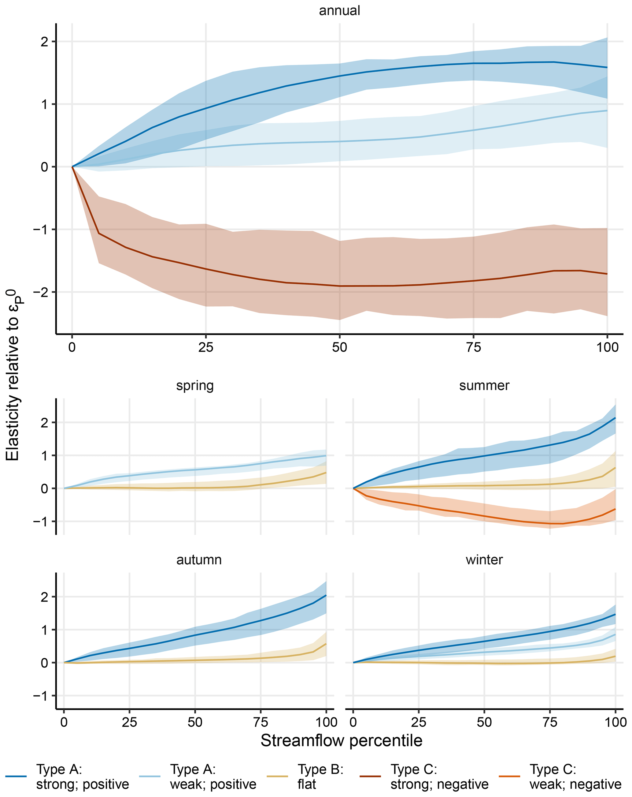
Figure 2Normalized elasticity curves that show the curves resulting from the single-catchment log-linear models (LMs), where each line represents the mean of the distribution of elasticity point estimates (for a cluster of sites) and each band represents the interquartile range. Note that spring and autumn have two clusters, while winter, summer, and annual have three, and that seasonal streamflow percentiles represent subsets of the annual flow.
At the annual timescale, 91 % of catchments exhibited type-A curves, demonstrating that in an overwhelming majority of cases, larger streamflow quantiles are proportionally more responsive to precipitation – 31 % of catchments (251) were grouped into a single class in which the average εc,P has a strongly positive slope (curve type A: strong), and 60 % of catchments (495) were clustered into a class in which said slope is weakly positive (curve type A: weak). In catchments with curve type A, where εc,P has a positive slope, higher streamflow percentiles are increasingly more responsive to a 1 % change in precipitation than low flows. Some catchments, predominantly in the eastern part of the country, exhibit different behaviour; 7 % of catchments (58) were clustered into a group with a strongly negative εc,P (curve type C: strong). A negatively sloping elasticity curve shape indicates that high flows are relatively less responsive to precipitation variation than lower flows. In other words, variation in precipitation predominantly affects the hydrologic response of higher streamflow percentiles for catchments with a positively sloping εc,P and affects lower streamflow percentiles for catchments with a negatively sloping εc,P.
In winter, autumn, and spring, none of the cluster-average elasticity curves are negatively sloping. Indeed, 31 % of catchments (246) in autumn, 26 % (211) in winter, and 65 % (524) in spring are grouped into a cluster in which εc,P can be described as relatively flat (curve type B), defined here as having a range of normalized values between −0.75 and positive 0.75. In winter, catchments with curve type B are mostly concentrated at high latitudes and in mountainous regions, while in autumn, these catchments are geographically more widespread (Fig. 3c), existing in the north, in the southwest, and to some extent along the Gulf Coast. A flat elasticity curve denotes a catchment in which the responsiveness of streamflow to changes in precipitation is consistent across the distribution. The remaining clusters have positively sloping curves. Similarly, 78 % of catchments (626) in the summer season exhibit curve type B. Meanwhile ∼ 14 % of catchments (111) exhibit curve type A (strongly positive), and the cluster with the remaining 8 % of catchments (68) generally has a negatively sloping curve (type C: weak). Finally, ∼ 35 % of catchments (281) in spring exhibit weakly positive curves (type A: weak). In spring, the absolute difference between the cluster-specific and across all curves is small, not exceeding 1 percentage point on average for any group.
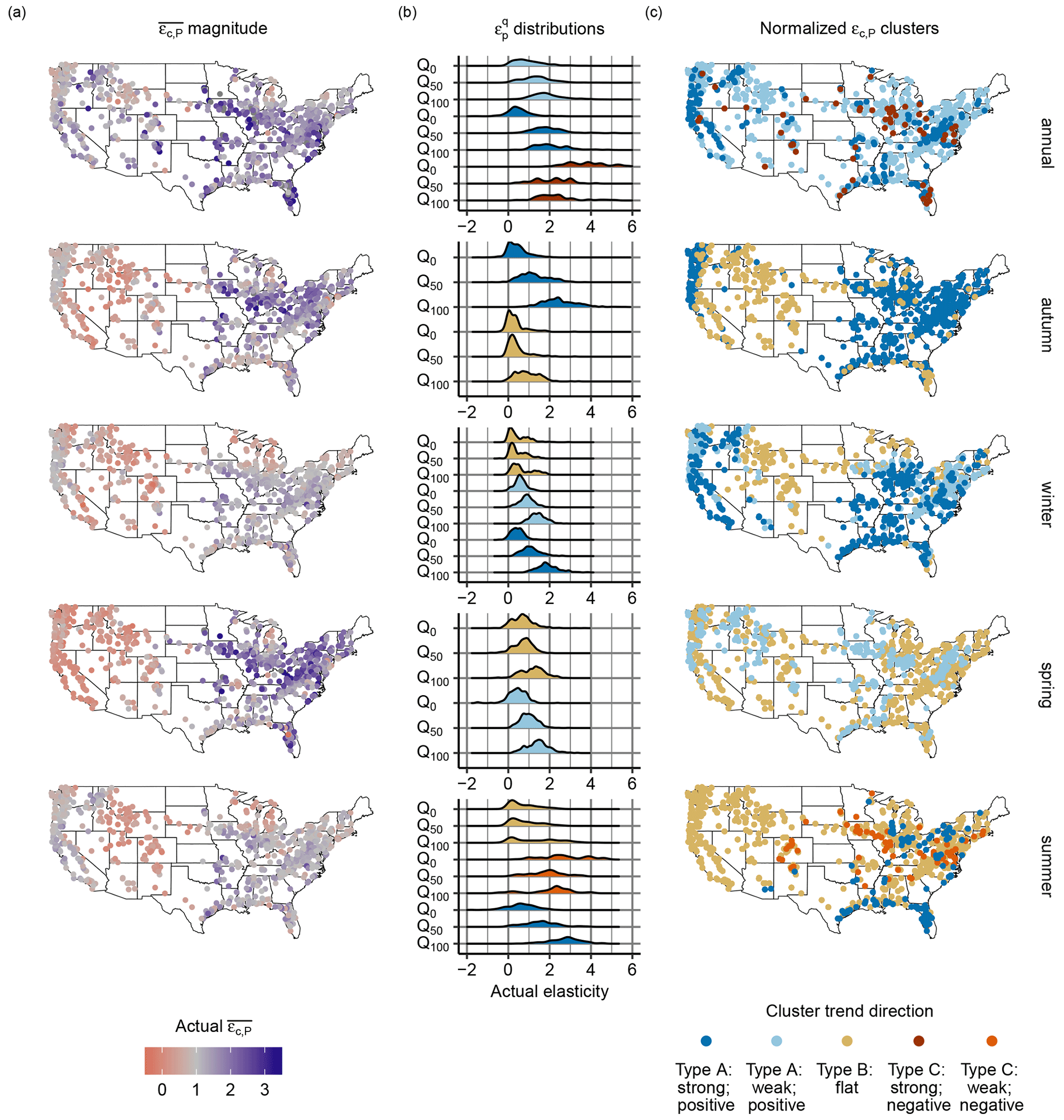
Figure 3Actual elasticity compared to normalized elasticity curves. Panel (a) shows the geographic distribution of the means of the non-normalized, site-specific elasticity curves. These values are referred to as actual-elasticity values in the text. Smaller mean-elasticity values (less responsive) are highlighted in lighter shades and higher mean-elasticity values in darker shades. Panel (b) shows the distributions for non-normalized point estimates of elasticity at the lowest, median, and highest streamflows (Q0, Q50, Q100) in each time period (annual, winter, spring, summer, autumn). The distributions in (b) are coloured according to the cluster membership of the normalized curves (Fig. 2), the geographic distribution of which is shown in (c).
Elasticity curve shape and the actual magnitude of expected streamflow change in response to a 1 % change in precipitation do not necessarily correspond (Fig. 3). For instance, in summer, 78 % of catchments exhibit a flat elasticity curve (Fig. 3a and c, summer). However, while skewed towards zero, the distribution of possible elasticity magnitude is widespread (Fig. 3b, summer), indicating that the streamflow response to a 1 % change in precipitation in this group ranges from between about 0 %–2 %. Conversely, the distributions of magnitude for flat elasticity curves in winter are concentrated around zero, indicating that streamflow across the majority of catchments has a very low responsiveness to precipitation variation in this season. In other words, a flat elasticity curve indicates that low and high flows have approximately the same response to precipitation changes within a particular catchment but that the response is not necessarily small or consistent across catchments with the same elasticity curve shape. The highest actual-elasticity values are predominantly in the eastern US in all seasons. High-magnitude elasticity values also occur in the Pacific Northwest, especially in the autumn, winter, and summer seasons.
It is worth noting that the distribution of streamflow in each season represents a subset of the streamflow in a year. For example, the streamflow magnitude which corresponds to high flows in the winter season may be equivalent to average or lower streamflow at the annual timescale.
3.2 Attribution and predictability of between-catchment variation in streamflow elasticity
We conduct a multivariate variable importance analysis using random forest models to determine the extent to which catchment attributes are able to predict elasticity curve shape. The following catchment characteristics are included in this analysis: the aridity index, the DFI, the BFI, the slope of the flow duration curve (calculated at the 0th–33rd, 33rd–66th, and 67th–100th percentiles), latitude, the coefficient of variation for daily streamflow in each season, mean annual temperature, mean catchment elevation, drainage area, mean catchment slope, and snow fraction, as well as precipitation and streamflow seasonality and timing metrics (Table B1). Averaged over 10 iterations each, the random forest model accurately predicted class membership in approximately 70 % of cases at the annual timescale, 95 % for autumn, 79 % for winter, 63 % for spring, and 79 % for summer, all rounded to the nearest integer.
For each temporal scale, different variables were selected as the best predictors of cluster membership using both the Gini coefficient and the mean decrease accuracy metric. For both the annual and summer periods, fdcbl was the best predictor for every iteration of the random forest model. At the annual timescale, the DFI, fdcb, and aridity were the second- and third-best predictors of cluster membership, depending on the model run. The second- and third-best predictors for summer class membership varied between iterations. For winter, the best predictors for both metrics were either average annual temperature or the time delay between the least important precipitation season and the low-streamflow season. In addition to these metrics, mean catchment elevation and other seasonality metrics were frequently selected as the second- or third-most important predictors for winter, depending on the model run. For autumn, the time delay between the least important precipitation season and the low-streamflow season, mean catchment elevation, and the BFI were the top three predictors in the majority of iterations of the model for both metrics and typically had very similar mean decrease accuracy scores and Gini coefficients. No variable was clearly the best predictor of cluster membership in springtime, as over the course of 10 model runs, eight different variables had the highest Gini coefficient or mean decrease accuracy score.
In this paper, we use multivariate statistical models to investigate whether streamflow elasticity to precipitation varies across the distribution of streamflow at annual and seasonal timescales. We then use a clustering algorithm and random forest regression model to examine the extent to which that variation is systematic and predictable.
By creating elasticity curves which represent the range of elasticity across the streamflow distribution (Fig. 2), we show that at annual and seasonal timescales, the highest streamflow percentiles are typically more responsive to long-term precipitation change compared to lower streamflow percentiles in the same catchment and time period. This is especially true for elasticity at the annual, spring, winter, and autumn timescales. The finding that low flows are less responsive to precipitation change than higher flows is in line with existing literature. Low flows are typically sustained by groundwater, saturated soils, and surface water storage, which require precipitation for recharge but for which the effects of changes in precipitation are inherently delayed and moderated (Gnann et al., 2021; Price, 2011; Smakhtin, 2001).
There are, however, catchments which do not have positively sloping elasticity curves at some timescales. Approximately 7 % of catchments at the annual timescale and 8 % in summer are clustered into groups with generally negative trends, indicating that low flows are relatively more responsive to precipitation than higher streamflow percentiles. Further, the elasticity curves of roughly 31 % of catchments in autumn, 78 % in summer, 65 % in spring, and 26 % in winter are nearly flat, with very low slopes for the majority of the curves and estimates only increasing marginally for the highest streamflow percentiles.
The best predictors of elasticity curve shape are those related to the hydrologic storage capacity of the catchments. For instance, fdcbl, the most important catchment attribute at the annual timescale and in summer, provides information about a catchment's ability to sustain flows of a certain magnitude during the dry season. The flow duration curve (fdc), here calculated using daily streamflow for the entire study period, is a cumulative frequency curve which shows the percentage of time that a certain magnitude of streamflow is equalled or exceeded (Searcy, 1959). When the slope of the fdc is steep, it indicates that a catchment has highly variable streamflow predominantly originating from direct runoff, and when the slope is relatively flat, it suggests the presence of surface or groundwater storage, which equalizes flow. At the low end of the fdc (here fdcbl), a flat slope points to the presence of long-term storage within the catchment, while a steep slope indicates that very little long-term storage exists (Searcy, 1959). Similarly, baseflow is the portion of streamflow that is derived from groundwater and other delayed sources (Smakhtin, 2001), and a low BFI indicates a catchment in which streamflow mostly comes from direct runoff. We have defined two baseflow metrics, the BFI and the DFI (a delayed-flow metric over a longer time span) (Gnann et al., 2021; Stoelzle et al., 2020), both of which are frequently important predictors of elasticity curve shape. Further, while snow fraction was not necessarily the most important predictor in cold months, temperature, latitude, elevation, and the time gap between the most important precipitation season and the most important streamflow season, attributes which relate to precipitation type and snow dominance, were.
Storage components consist of anything ranging from surface waterbodies such as wetlands to snow cover and groundwater influxes, all of which interact with fluvial systems at different timescales. Catchments with relatively flat elasticity curves in cold months (winter and autumn) are typically those at high latitudes which receive higher percentages of precipitation as snow or those in the semi-arid southwestern region which are predominantly fed by snowmelt upstream (Li et al., 2017). These curves are flat and have actual-elasticity estimates which are heavily skewed towards zero (winter and autumn, Fig. 3a and b) because snowmelt does not usually occur in winter or autumn. However, at the annual timescale, the same catchments have actual-elasticity values ranging from less than 1 for low flows to around 2 for the highest annual flows because the streamflow response is delayed but occurs within the same year. In autumn, there are additionally catchments in Florida and scattered along the southern coast with relatively flat elasticity curves, potentially due to increased storage within the catchment area, e.g. in wetlands. The seasonal elasticity estimates specifically capture the influence of in-season precipitation on streamflow within that same season. Streamflow in many rivers is driven by out-of-season precipitation. Thus, while flat seasonal elasticity curves and low percentile-specific point estimates indicate a muted hydrologic response, they do not rule out the possibility that the timescale for response is merely longer than that which is considered. Further, as noted previously, seasonal flow percentiles represent sub-samples of annual flow. These may or may not directly correspond to the same section of the flow distribution. For instance, the 50th percentile of summer flow may relate to a much lower or higher annual flow percentile, depending on the temporal distribution of flow in the year.
Flat elasticity curves are present across most of the country during summer (Fig. 2, summer; Fig. 3c), indicating that the response of streamflow to summer precipitation is similar across all flow percentiles in these catchments. Similar to those in winter and autumn, the flat elasticity curves in summer tend to have higher BFI and DFI values and lower fdcbl values than type-A or type-C curves. Many of these catchments have average actual-elasticity values which approximate 0, indicating that in-season precipitation has little to no influence on seasonal streamflow; however, others have larger average actual-elasticity values, often greater than 1 (Fig. 3a and b, summer), which, in turn, implies summer precipitation has a substantial influence on summer streamflow but that the influence is consistent across the distribution. This differs from a majority of cases in other seasons and at the annual timescale, in which the influence of precipitation on streamflow is magnified in higher streamflow percentiles.
Evidence suggests that high flow magnitudes are driven by the combined influences of precipitation events and antecedent soil moisture (Ivancic and Shaw, 2015; Slater and Villarini, 2016b). Summer is a period of relative soil moisture deficit (Koehn et al., 2021) and high potential evaporation. It is plausible, therefore, that the non-zero-magnitude flat elasticity curves in most of the study region during this period are emblematic of the relationship between antecedent wetness, precipitation, and streamflow. In other words, because of a soil moisture deficit, the precipitation changes are not typically magnified at higher streamflow percentiles in the majority of catchments (78 %) during this period, especially in catchments where sources of delayed flow (e.g. groundwater) are large contributors across the flow distribution (Berghuijs and Slater, 2023).
This does not, however, explain the relative homogenization of the elasticity curve structure in spring, a period in which soil moisture recharge is likely to occur. Instead, it seems probable that the flatness of the elasticity curve shape, despite a persistently broad range of elasticity magnitudes in spring (Fig. 3 spring: B), may be due to the fact that streamflow is less variable on average in springtime compared to the other seasons, as determined by the coefficient of variation (CV) of the daily streamflow measurements, and that springtime is the low-flow season in only 24 catchments. In other words, the lowest flows in spring may be more heavily driven by runoff from precipitation rather than storage as compared to other seasons. This hypothesis is further supported by the cluster-specific CV distributions at other timescales – where type-B elasticity curves correspond to catchments with relatively low variability (Fig. 4, spring). The shape may also reflect, in part, the climatic drivers dominant over different regions.
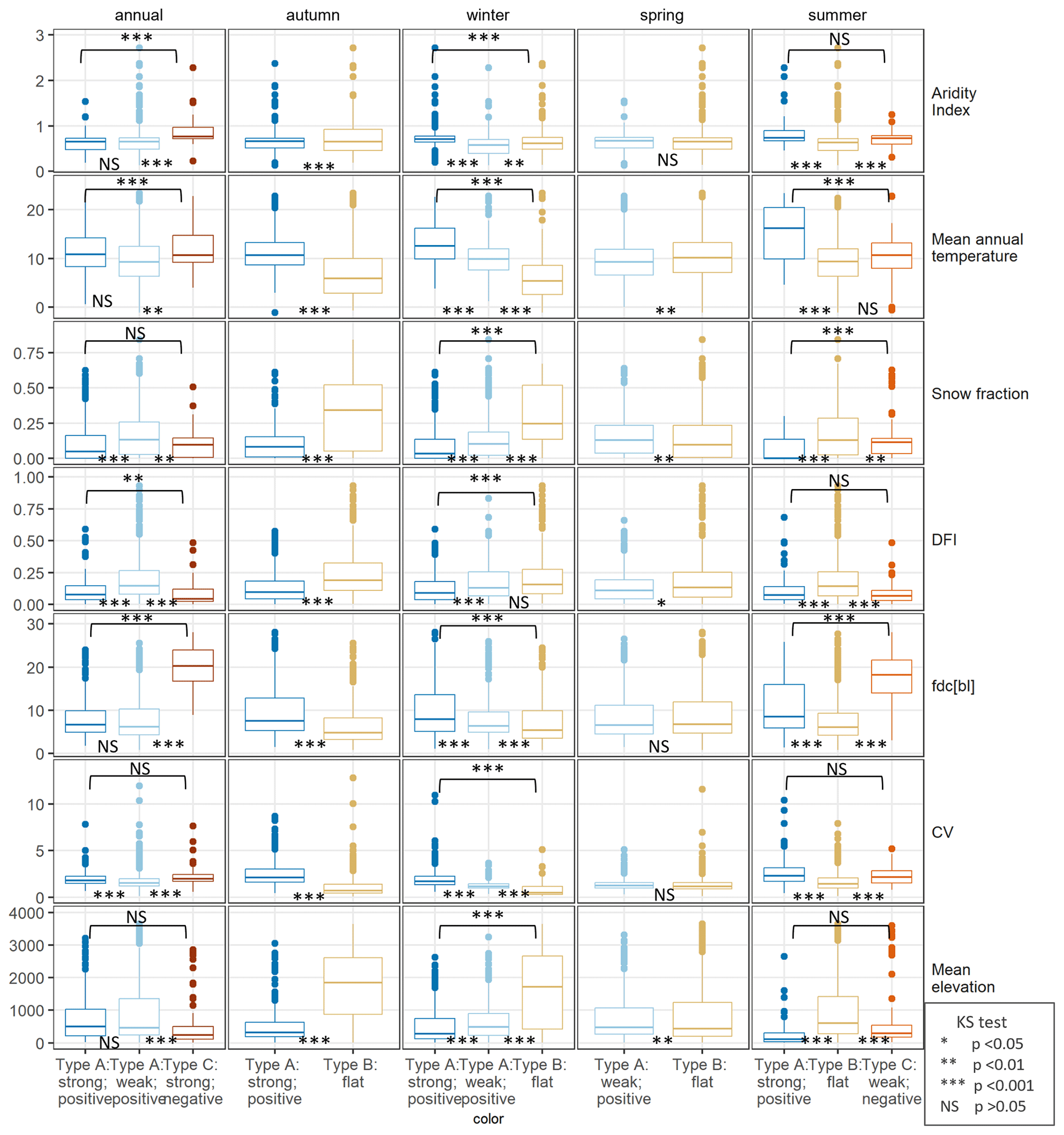
Figure 4Boxplots showing the distributions of static catchment attributes split by time period and cluster membership. Significance is shown between each box for neighbouring distribution plots, and the significance of the difference between the first and last distribution in each time period is plotted at the top of the panel (annual, winter, and summer) – note that NS means not significant. Boxplots are included for attributes which are important in the random forest (RF) analysis and can be represented by continuous numeric values, so seasonality metrics are excluded here.
The range of type-B elasticity curves which is present across the seasons is washed out at the annual scale, demonstrating that the catchment storage which leads to a uniform response across the distribution of streamflow generally operates at a timescale of less than a year (Fig. 2). Type-A elasticity curves with a strong signal exist across temporal scales in catchments which have a relatively low BFI and DFI and steep middle sections of the flow duration curve, fdcb, as compared to type-B and weak type-A curves (Fig. 4). Interestingly, at the annual timescale, catchments exhibiting curve type C (negative) are in some ways similar to those with strong signals from curve type A (positive) in that they both have low snow fraction, a low BFI, and steep fdcb slopes. They differ, however, in a number of other attributes, most notably the DFI and the slope of the low end of the flow duration curve, fdcbl. This difference indicates that while streamflow in catchments exhibiting both types of curves is predominantly rain-fed, those exhibiting strong type-A curves are better able to sustain low flows as compared to catchments with type-C curves. Catchments with type-C curves have very flashy low-flow behaviour. We controlled for ephemeral streams in this study in order to simplify our methodology, but including those catchments may increase the prevalence of type-C curves. The type-C elasticity curves have wide interquartile ranges and wide confidence intervals when estimated with a panel regression model (Fig. B1), indicating lower robustness in the estimation of this group overall (Fig. 2). The strong type-C cluster at the annual timescale also exhibits a positive slope above the 35th percentile of streamflow. While speculative, these results suggest that type-C curves may differ from positive instances of εc,P predominantly in that they exhibit highly flashy low-flow behaviour (Fig. 4).
4.1 Example catchments and limitations
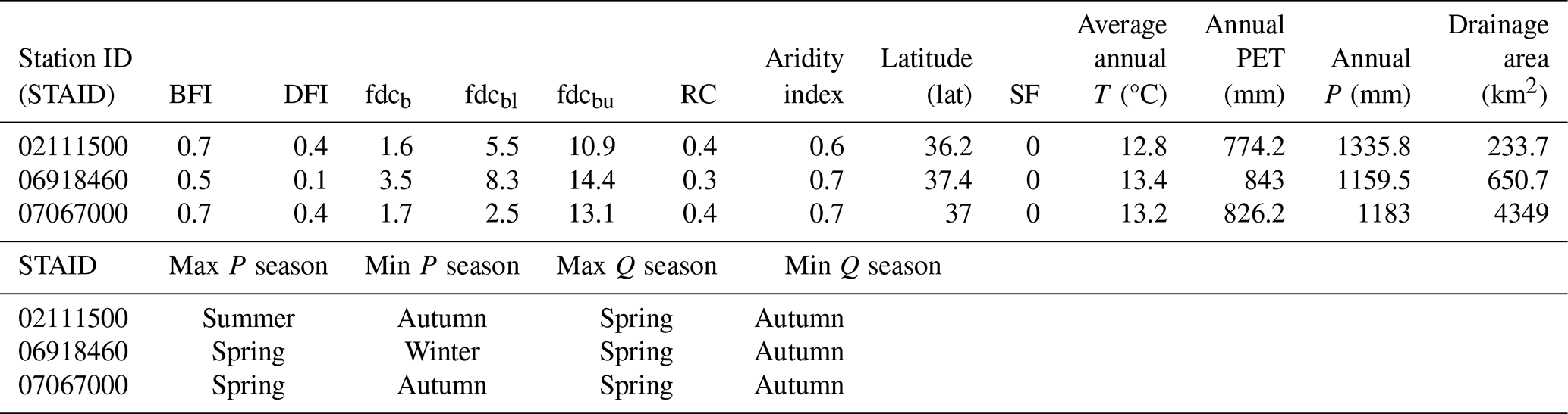
In order to contextualize the approach at individual locations, we examine the elasticity curves of three streamflow gauges. The non-normalized elasticity curves for Turnback Creek above Greenfield, MO (gauge ID: 06918460); Current River at Van Buren, MO (gauge ID: 07067000); and Reddies River at North Wilkesboro, NC (gauge ID: 02111500) are included in Fig. 5. Despite being located near one another, gauge station 07067000 lies over the Ozark Plateaus aquifer, a more mature karstic environment with more long-term storage and a higher DFI (0.4) and BFI (0.7) as compared to gauge station 06918460 (DFI: 0.1; BFI: 0.5) (Gnann et al., 2021). Conversely, gauge station 02111500 is physically distant from the other two catchments and has a different geological profile (Zimmer and Gannon, 2018) but has substantial seasonal and stable storage components resulting in high DFI (0.4) and BFI (0.7) values compared to both of the Ozarks catchments. Catchment attributes for each of these sites are presented in Table 1.
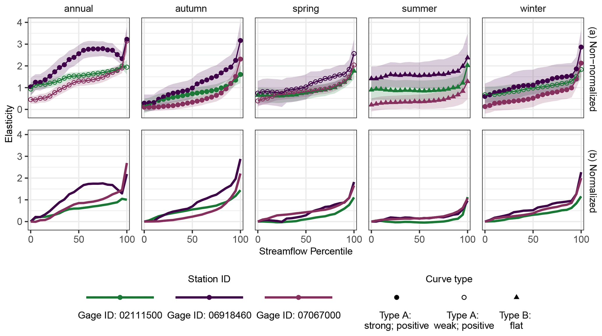
Figure 5Examples of elasticity curves from three example catchments: Turnback Creek above Greenfield, MO (gauge ID: 06918460); Current River at Van Buren, MO (gauge ID: 07067000); and Reddies River at North Wilkesboro, NC (gauge ID: 02111500). Panel (a) shows the non-normalized curves to demonstrate actual elasticity, and panel (b) shows the normalized curves to demonstrate the similarity in curve form. Catchments located near one another geographically are both represented in shades of purple. Point shape represents the curve type, and the bands represent the 95 % confidence intervals. Points and confidence intervals have been removed from (b) to improve visibility, but the curve types and confidence bands are consistent across both panels.
At the seasonal timescale, both of the Ozarks catchments (Fig. 5, in purple) are consistently classified as the same curve type. However, several things are apparent. First, in a non-normalized format, as presented in panel (a) of Fig. 5, it is clear that the catchment with young karstic geology (06918460) and less long-term storage experiences a higher absolute magnitude of elasticity to precipitation (Fig. 5a) when compared to its counterpart. This is particularly clear in summer, when the curve shape is similar (Fig. 5b) but the estimated magnitude of elasticity differs by more than 1 percentage point. Second, despite having relatively similar curves at the seasonal timescale, these two catchments exhibit different behaviour at the annual timescale, at which 06918460 has a strongly positive signal and 07067000 has a weakly positive signal, demonstrating the association between increased long-term storage and a less steeply sloping elasticity curve. At the annual timescale, the elasticity curves of these two catchments demonstrate the nuance required in interpreting the classification system – both curves span a similar total range of elasticity. However, the overall condition of the strongly positive curve (06918460) is steeper, as a large portion of the increase in the elasticity curve for 07067000 occurs between the 95th and 100th flow percentiles. Further, the more physically distant catchment (02111500; Fig. 5, represented in green) has relatively similar characteristics to 07067000 (Fig. 5; Table 1) and exhibits a similar curve structure at the annual and seasonal timescales, although with a slightly flatter overall condition.
Table 1Attributes of example catchments: Turnback Creek above Greenfield, MO (gauge ID: 06918460); Current River at Van Buren, MO (gauge ID: 07067000); and Reddies River at North Wilkesboro, NC (gauge ID: 02111500). Definitions of attributes are included in Table B1. Max and min P season are the most and least important precipitation seasons respectively, and max and min Q season are the most and least important flow seasons respectively.
Informative in the aggregate, the elasticity curve concept is limited in several ways, some of which are apparent in these examples. First, while curve shape is approximately consistent within the clusters, there is a margin of error around the groupings. The choice of the number of clusters per temporal scale was carefully considered in the interest of parsimony, so some catchments inevitably exhibit behaviour outside of the norm. Further, the shapes of the curves are not always smooth, as is evident in the example catchment 06918460, where a substantial decrease in elasticity is evident between the 80th and 95th percentiles at the annual timescale. The intention of this paper is to introduce the concept in a large-sample context, and additional research is needed to determine the extent to which minor variations in shape may be due to statistical noise or physical processes. Thus, the suitability of the concept for application at small scales remains to be established.
The LM-constructed curves or point estimates in individual catchments may deviate substantially from the cluster average, may comprise insignificant point estimates, or may violate assumptions of the regression approach used. For instance, depending on the streamflow percentile, the residuals of the single-catchment LMs between 68 % ( and 78 % ( were normally distributed as estimated by a Shapiro–Wilk test with an alpha level of 0.01, and those between 75 % ( and 80 % ( had a Durbin–Watson test statistic of greater than 1, indicating that autocorrelation was not a serious concern at these sites. This means that the normality assumption was violated in around 20 % to 30 % of catchments and the non-autocorrelation assumption was violated in 20 % to 25 % of catchments. The fixed-effects panel regression approach (Appendix A and Fig. B1) helps to mitigate these concerns, lending credibility to the aggregated curves, but the reader is cautioned that application at the scale of a single catchment may carry substantial uncertainty. Further, the single-catchment multivariate regression approach which we have taken here is a standard method for calculating point estimates of elasticity; however, this approach does not accommodate the possibility of non-linear elasticity, e.g. the possibility that a 1 % and a 10 % difference in precipitation are not linearly related. This work only considers the elasticity of streamflow magnitude, a singular component of streamflow which may not fully capture the influence of precipitation variability. Finally, the selected clusters depict whether curves are generally increasing or decreasing but do not account for the exact shape of the curves themselves; for instance, they do not depict at which percentiles the slope begins to increase or decrease. In some instances, the curves for individual sites do not align with the precise curve types according to which we have named the clusters. For instance, while the average curve in a cluster may be “type A: strong”, an individual curve may be “type A: weak”. For this reason, we have presented the single-catchment data with the interquartile ranges of curve estimates and recommend caution when estimating elasticity curves or even elasticity magnitude for individual locations.
The work presented in this paper represents an introduction to elasticity curves. This concept may support further research into understanding how changes in water storage might affect streamflow response over time (Saft et al., 2016, 2015) and how groundwater contributes to flood generation (Berghuijs and Slater, 2023), and it provides insight into the implications of climate change for the hydrological cycle and the rainfall–runoff relationship. Further, we include panel regression models as a tool for more robust elasticity estimation (Appendix A) – a method which may be well suited to the regional calculation of elasticity and estimation in ungauged basins.
In this paper, we introduce a new concept for understanding and classifying streamflow response to precipitation. Representing streamflow elasticity to precipitation as a curve which reflects the range of responses across the distribution of streamflow within a given time period, instead of as a single-point estimate, provides a novel lens through which we can interpret hydrological behaviour. We have shown that εP estimated from the central summary of streamflow, e.g. the annual median, does not provide a complete picture of streamflow change. We have demonstrated that elasticity curve shape, i.e. the response of different flow percentiles relative to one another in a given catchment, can be understood separately from between-catchment variation in the magnitude of streamflow elasticity associated with a 1 % change in precipitation.
We identify three typical elasticity curve shapes:
-
In type A, low flows are the least responsive and high flows are the most responsive. The majority of catchments at the annual, winter, and autumn timescales exhibit this behaviour.
-
In type B, the response is relatively consistent across the flow distribution. At the seasonal timescale, many catchments experience a consistent level of response across the flow regime. This is especially true in snow-fed catchments during cold months, when the actual elasticity skews towards zero for all flow percentiles while precipitation is held in storage. A consistent response is seen across most of the country during spring, when streamflow is comparatively stable and rainfall-driven, and in summer, when evaporative demand is high and soil moisture is low.
-
In type C, low flows are the most responsive to precipitation change. These catchments are dominated by highly flashy low-flow behaviour.
Depending on the timescale examined, annual or seasonal, we predict elasticity curve type with fairly high accuracy, ranging from 95 % in autumn to 63 % in spring, using catchment characteristics and other hydrologic signatures. The best predictors of curve type include the low end of the slope of the flow duration curve, mean annual temperature, seasonality, mean catchment elevation, and the baseflow index. All of these attributes relate to hydrological storage and release timing.
Panel model design
In order to further validate the elasticity estimates, we constructed a fixed-effects panel regression model (Eq. A1) for each timescale (. The panel models were designed to control for confounding variables, and the clusters established from the LM results were included as interaction terms to help explain the variation in elasticity curve shape. A confounding variable is an attribute of a catchment or group of catchments which could influence both the dependent variable and the independent variable, causing a spurious association.
Time-invariant confounders at the catchment scale are controlled for by the stream-gauge-specific intercept αi. At the timescale of this study (30–39 years of data per site), the majority of confounding variables at the catchment scale may be reasonably expected to be time-invariant (e.g. topography). While some land cover changes are likely to occur over the time period, a minority of catchments are likely to have experienced large percentages of detectable land cover change, and, when considered jointly in a panel model, the effects of land cover changes on streamflow are likely to be small relative to climatic effects (Anderson et al., 2022). Variables such as temperature and actual evaporation are partially or fully considered through the calculation or inclusion of other variables. More complex formulations of the panel model, which explicitly included ecoregions and/or a control for time-varying confounders at the national scale, were considered; however, the resulting curves were not substantially different from one another, and thus the simplest model (Eq. A1) is used. The panel model is represented by
where is the natural logarithm of the streamflow percentile (q) calculated for time period (t) for catchment (i), αi,t is the stream-gauge-specific intercept, ln(Pi,t) is the logarithm of catchment-averaged daily precipitation, and ln(Ei,t) is the logarithm of catchment-averaged daily potential evaporation. The elasticity curve cluster for each catchment is represented by a categorical variable (g), and ln(Pi,t)gi and ln(Ei,t)gi are interaction terms between the assigned cluster and precipitation or potential evaporation. Precipitation elasticity, the effect measured by this model, is represented by the regression coefficient , and potential evaporation elasticity is represented by . The error term is . Autocorrelation in fixed-effects panel models can lead to the underestimation of standard errors. We address this concern by clustering standard errors at the stream-gauge level as in Anderson et al. (2022). The panel regression results are normalized following the same procedure as that for the LMs – by subtracting from each value.
The panel regression models are included as a more robust method of estimation and as a tool for confirming the results of the individual regression models. The results of these models were not included in the main text because they do not differ substantially from those of the simpler regression approach. They are included here in the appendix because longitudinal regression approaches, such as panel regression models, are substantially more robust when averages are of interest and lend credibility to the outcomes of the analysis.
The curves in Fig. B1 were produced using the panel regression approach (Eq. A1) and are plotted with the normalized 95 % confidence intervals of the panel model. The panel regression model results in one estimated elasticity value for each percentile and allows for easy calculation of statistical uncertainty.
The point estimates are all significant at the 99.99 % confidence level. The interactions are also significant at the 99.99 % confidence level, except for annual streamflow above the 65th percentile, where all interactions are significant at the 95 % confidence level at least, except for the highest annual flow (100th percentile), at which the interaction is not significant. This means that the estimates are statistically significantly different from one another for each of the clusters at every temporal scale and every percentile, with the exception of the highest annual streamflow. The actual magnitude of the elasticity estimates for the maximum annual streamflow is not statistically different across the groups (Fig. 3, annual).
Table B1Descriptions of the catchment attributes considered in the explanatory analysis.
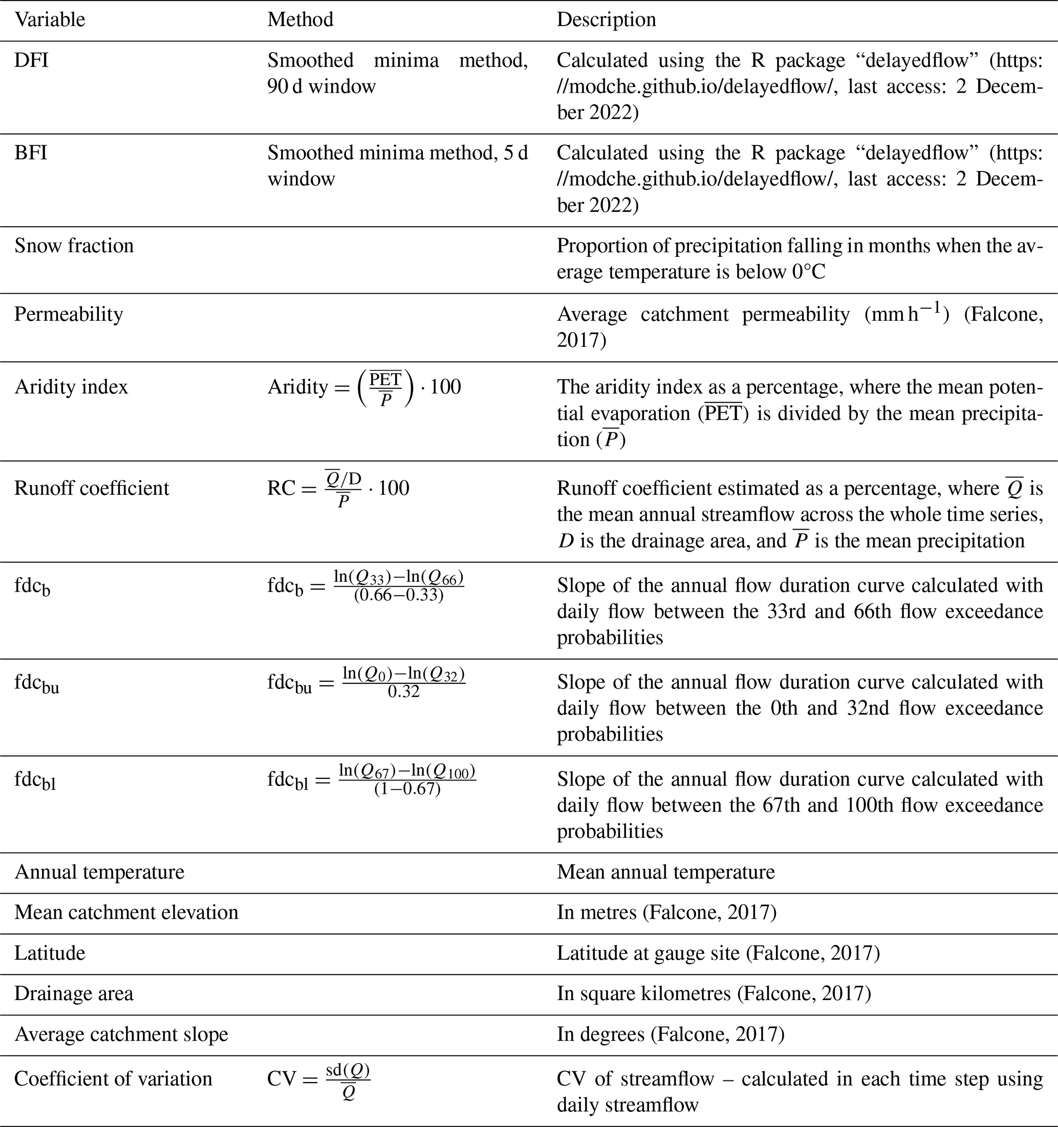
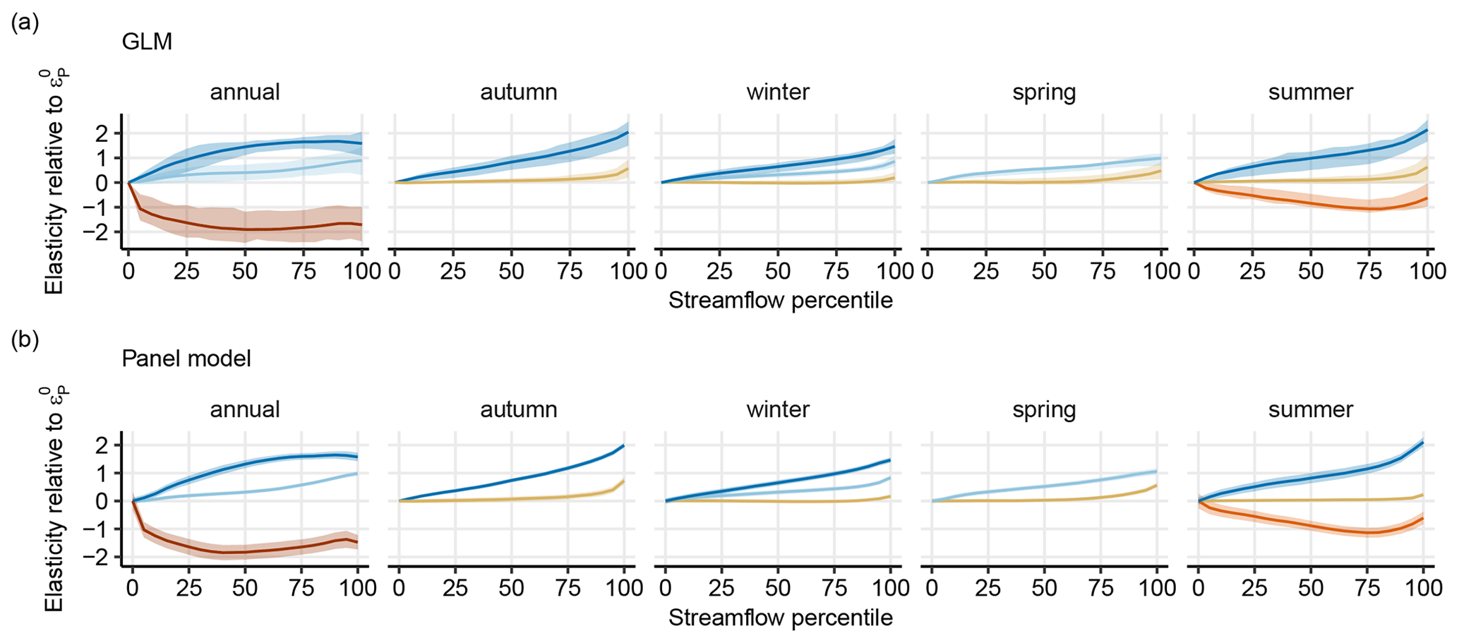
Figure B1Elasticity curves estimated using the single-site regression models (a) and the aggregated panel regression models described in Appendix A (b). Generalized linear models (GLMs) are each presented with the interquartile range of all estimates, and panel models are presented with the 95 % confidence intervals. Panel (a) is duplicated from Fig. 2 here to facilitate comparison.
All data used in this study come from secondary datasets which are publicly available at the time of publication. Data regarding total upstream dam storage, average annual runoff, drainage area, mean catchment elevation, latitude, and average catchment slope are available through the GAGES II dataset at https://doi.org/10.3133/70046617 (Falcone, 2011). Watershed boundaries are also available through the GAGES II dataset at https://doi.org/10.5066/F7HQ3XS4 (Falcone, 2017). Climate data are available from PRISM at https://prism.oregonstate.edu (PRISM Climate Group, 2014) nd can be downloaded using the R package “prism” (Edmund and Bell, 2020). Streamflow data can be downloaded from the National Water Information System (NWIS) using the R package “dataRetrieval” (DeCicco et al., 2024). R code for the complete analysis has been available since 2 December 2022 at https://doi.org/10.5281/zenodo.7391227 (Anderson, 2022).
The conceptualization and methodology were designed by BJA, MIB, and LJS. Data curation, formal analysis, investigation, project administration, software handling, visualization, and writing (original draft preparation) were performed by BJA. Supervision and validation were carried out by LJS, SJD, and MIB. Writing (review and editing) was carried out by LJS, SJD, MIB, and BJA.
At least one of the co-authors is a member of the editorial board of Hydrology and Earth System Sciences. The peer-review process was guided by an independent editor, and the authors also have no other competing interests to declare.
Publisher’s note: Copernicus Publications remains neutral with regard to jurisdictional claims made in the text, published maps, institutional affiliations, or any other geographical representation in this paper. While Copernicus Publications makes every effort to include appropriate place names, the final responsibility lies with the authors.
We thank the attendees of the STAHY2022 workshop, the hydrology research group at the University of Freiburg, and the water lab at the University of Oxford, as well as Ross Woods and Linda Speight for their valuable input. In particular, we thank Richard Vogel, Michael Stoelzle, Markus Weiler, and Kerstin Stahl, whose comments led to methodological and conceptual improvements in this work. Bailey J. Anderson thanks the Clarendon Scholarship and Hertford College, Oxford, for financial support during her PhD.
This research has been supported by UK Research and Innovation (grant no. MR/V022008/1).
This paper was edited by Thom Bogaard and reviewed by Keirnan Fowler and one anonymous referee.
Allaire, M. C., Vogel, R. M., and Kroll, C. N.: The hydromorphology of an urbanizing watershed using multivariate elasticity, Adv. Water Resour., 86, 147–154, https://doi.org/10.1016/j.advwatres.2015.09.022, 2015.
Anderson, B.: bails29/Elasticity_curve_analysis: initial release of code for generating and analysing elasticity curve data (v1.1), Zenodo [code], https://doi.org/10.5281/zenodo.7391227, 2022.
Anderson, B. J., Slater, L. J., Dadson, S. J., Blum, A. G., and Prosdocimi, I.: Statistical Attribution of the Influence of Urban and Tree Cover Change on Streamflow: A Comparison of Large Sample Statistical Approaches, Water Resour. Res., 58, e2021WR030742, https://doi.org/10.1029/2021WR030742, 2022.
Andréassian, V., Coron, L., Lerat, J., and Le Moine, N.: Climate elasticity of streamflow revisited – an elasticity index based on long-term hydrometeorological records, Hydrol. Earth Syst. Sci., 20, 4503–4524, https://doi.org/10.5194/hess-20-4503-2016, 2016.
Bassiouni, M., Vogel, R. M., and Archfield, S. A.: Panel regressions to estimate low-flow response to rainfall variability in ungaged basins, Water Resour. Res., 52, 9470–9494, https://doi.org/10.1002/2016WR018718, 2016.
Berghuijs, W. R. and Slater, L. J.: Groundwater shapes North American river floods, Environ. Res. Lett., 18, 034043, https://doi.org/10.1088/1748-9326/acbecc, 2023.
Berghuijs, W. R., Larsen, J. R., van Emmerik, T. H. M., and Woods, R. A.: A Global Assessment of Runoff Sensitivity to Changes in Precipitation, Potential Evaporation, and Other Factors, Water Resour. Res., 53, 8475–8486, https://doi.org/10.1002/2017WR021593, 2017.
Blum, A. G., Ferraro, P. J., Archfield, S. A., and Ryberg, K. R.: Causal Effect of Impervious Cover on Annual Flood Magnitude for the United States, Geophys. Res. Lett., 47, e2019GL086480, https://doi.org/10.1029/2019GL086480, 2020.
Brunner, M. I., Swain, D. L., Gilleland, E., and Wood, A. W.: Increasing importance of temperature as a contributor to the spatial extent of streamflow drought, Environ. Res. Lett., 16, 024038, https://doi.org/10.1088/1748-9326/abd2f0, 2021.
Chiew, F.: Estimation of rainfall elasticity of streamflow in Australia, Hydrolog. Sci. J., 51, 612–625, https://doi.org/10.1623/hysj.51.4.613, 2006.
Chiew, F., Peel, M., McMahon, T., and Siriwardena, L.: Precipitation elasticity of streamflow in catchments across the world, Clim. Var. Chang. Impacts Proc. Fifth FRIEND World Conf, November 2006, Havana, Cuba, 308, 256–262, 2006.
Cooper, M. G., Schaperow, J. R., Cooley, S. W., Alam, S., Smith, L. C., and Lettenmaier, D. P.: Climate Elasticity of Low Flows in the Maritime Western U.S. Mountains, Water Resour. Res., 54, 5602–5619, https://doi.org/10.1029/2018WR022816, 2018.
Croissant, Y. and Millo, G. (Eds.): Endogeneity, in: Panel Data Econometrics with R, John Wiley & Sons, Ltd, Chichester, UK, 139–159, https://doi.org/10.1002/9781119504641.ch6, 2018.
DeCicco, L., Hirsch, R., Lorenz, D., Watkins, D., and Johnson, M.: dataRetrieval: Retrieval Functions for USGS and EPA Hydrologic and Water Quality Data [code], US Geological Survey [code], https://doi.org/10.5066/P9X4L3GE, 2024.
Edmund, H. and Bell, K.: prism: Access Data from the Oregon State Prism Climate Project [code], Oregon State PRISM Project, Zenodo [code], https://doi.org/10.5281/zenodo.33663, 2015.
Falcone, J. A.: GAGES-II: Geospatial Attributes of Gages for Evaluating Streamflow, USGS [data set], https://doi.org/10.3133/70046617, 2011.
Falcone, J. A.: U.S. Geological Survey GAGES-II time series data from consistent sources of land use, water use, agriculture, timber activities, dam removals, and other historical anthropogenic influences, US Geological Survey [data set], https://doi.org/10.5066/F7HQ3XS4, 2017.
François, B., Schlef, K. E., Wi, S., and Brown, C. M.: Design considerations for riverine floods in a changing climate – A review, J. Hydrol., 574, 557–573, https://doi.org/10.1016/j.jhydrol.2019.04.068, 2019.
Gnann, S. J., McMillan, H. K., Woods, R. A., and Howden, N. J. K.: Including Regional Knowledge Improves Baseflow Signature Predictions in Large Sample Hydrology, Water Resour. Res., 57, e2020WR028354, https://doi.org/10.1029/2020WR028354, 2021.
Hamon, W. R.: Computation of direct runoff amounts from storm rainfall, Int. Assoc. Sci. Hydrol. Publ., 63, 52–62, 1963.
Harman, C. J., Troch, P. A., and Sivapalan, M.: Functional model of water balance variability at the catchment scale: 2. Elasticity of fast and slow runoff components to precipitation change in the continental United States, Water Resour. Res., 47, 1–12, https://doi.org/10.1029/2010WR009656, 2011.
Hodgkins, G. A., Dudley, R. W., Archfield, S. A., and Renard, B.: Effects of climate, regulation, and urbanization on historical flood trends in the United States, J. Hydrol., 573, 697–709, https://doi.org/10.1016/j.jhydrol.2019.03.102, 2019.
Hsiao, C.: Panel Data Analysis – Advantages and Challenges, TEST, 16, 1–22, https://doi.org/10.1007/s11749-007-0046-x, 2007.
Ivancic, T. J. and Shaw, S. B.: Examining why trends in very heavy precipitation should not be mistaken for trends in very high river discharge, Clim. Change, 133, 681–693, https://doi.org/10.1007/s10584-015-1476-1, 2015.
Koehn, C. R., Petrie, M. D., Bradford, J. B., Litvak, M. E., and Strachan, S.: Seasonal Precipitation and Soil Moisture Relationships Across Forests and Woodlands in the Southwestern United States, J. Geophys. Res.-Biogeosci., 126, e2020JG005986, https://doi.org/10.1029/2020JG005986, 2021.
Kormos, P. R., Luce, C. H., Wenger, S. J., and Berghuijs, W. R.: Trends and sensitivities of low streamflow extremes to discharge timing and magnitude in Pacific Northwest mountain streams, Water Resour. Res., 52, 4990–5007, https://doi.org/10.1002/2015WR018125, 2016.
Li, D., Wrzesien, M. L., Durand, M., Adam, J., and Lettenmaier, D. P.: How much runoff originates as snow in the western United States, and how will that change in the future?, Geophys. Res. Lett., 44, 6163–6172, https://doi.org/10.1002/2017GL073551, 2017.
Lu, J., Sun, G., McNulty, S. G., and Amatya, D. M.: A Comparison of Six Potential Evapotranspiration Methods for Regional Use in the Southeastern United States1, JAWRA J. Am. Water Resour. Assoc., 41, 621–633, https://doi.org/10.1111/j.1752-1688.2005.tb03759.x, 2007.
Milly, P. C. D., Kam, J., and Dunne, K. A.: On the Sensitivity of Annual Streamflow to Air Temperature, Water Resour. Res., 54, 2624–2641, https://doi.org/10.1002/2017WR021970, 2018.
Murtagh, F. and Contreras, P.: Algorithms for hierarchical clustering: an overview, WIREs Data Min. Knowl. Discov., 2, 86–97, https://doi.org/10.1002/widm.53, 2012.
Nichols, A.: Causal Inference with Observational Data, Stata J., 7, 507–541, https://doi.org/10.1177/1536867X0800700403, 2007.
Patil, S. and Stieglitz, M.: Hydrologic similarity among catchments under variable flow conditions, Hydrol. Earth Syst. Sci., 15, 989–997, https://doi.org/10.5194/hess-15-989-2011, 2011.
Potter, N. J., Petheram, C., and Zhang, L.: Sensitivity of streamflow to rainfall and temperature in south-eastern Australia during the Millennium drought, in: 19th International Congress on Modelling and Simulation, December 2011, Perth, 3636–3642, http://www.mssanz.org.au/modsim2011/I6/potter.pdf (last access: 5 April 2024), 2011.
Price, K.: Effects of watershed topography, soils, land use, and climate on baseflow hydrology in humid regions: A review, Prog. Phys. Geogr., 35, 465–492, https://doi.org/10.1177/0309133311402714, 2011.
PRISM Climate Group: PRISM recent years, Oregon State University, https://prism.oregonstate.edu, 2014.
Prudhomme, C., Crooks, S., Kay, A. L., and Reynard, N.: Climate change and river flooding: part 1 classifying the sensitivity of British catchments, Clim. Change, 119, 933–948, 2013.
Saft, M., Western, A. W., Zhang, L., Peel, M. C., and Potter, N. J.: The influence of multiyear drought on the annual rainfall-runoff relationship: An Australian perspective, Water Resour. Res., 51, 2444–2463, https://doi.org/10.1002/2014WR015348, 2015.
Saft, M., Peel, M. C., Western, A. W., and Zhang, L.: Predicting shifts in rainfall-runoff partitioning during multiyear drought: Roles of dry period and catchment characteristics, Water Resour. Res., 52, 9290–9305, https://doi.org/10.1002/2016WR019525, 2016.
Sankarasubramanian, A., Vogel, R. M., and Limbrunner, J. F.: Climate elasticity of streamflow in the United States, Water Resour. Res., 37, 1771–1781, https://doi.org/10.1029/2000WR900330, 2001.
Schaake, J. C.: From climate to flow, in: Climate change and US water resources, vol. 8, John Wiley and Sons Inc., New York, USA, 177–206, ISBN 978-0-471-61838-6, 1990.
Searcy, J. K.: Flow-duration curves, Water Supply Paper, U.S. Govt. Print. Off., https://doi.org/10.3133/wsp1542A, 1959.
Slater, L. J. and Villarini, G.: Recent trends in U.S. flood risk, Geophys. Res. Lett., 43, 12428–12436, https://doi.org/10.1002/2016GL071199, 2016a.
Slater, L. J. and Villarini, G.: Recent trends in U.S. flood risk, Geophys. Res. Lett., 43, 12428–12436, https://doi.org/10.1002/2016GL071199, 2016b.
Smakhtin, V. U.: Low flow hydrology: a review, J. Hydrol., 240, 147–186, https://doi.org/10.1016/S0022-1694(00)00340-1, 2001.
Stoelzle, M., Schuetz, T., Weiler, M., Stahl, K., and Tallaksen, L. M.: Beyond binary baseflow separation: a delayed-flow index for multiple streamflow contributions, Hydrol. Earth Syst. Sci., 24, 849–867, https://doi.org/10.5194/hess-24-849-2020, 2020.
Tang, Y., Tang, Q., Wang, Z., Chiew, F. H. S., Zhang, X., and Xiao, H.: Different Precipitation Elasticity of Runoff for Precipitation Increase and Decrease at Watershed Scale, J. Geophys. Res.-Atmos., 124, 11932–11943, https://doi.org/10.1029/2018JD030129, 2019.
Tang, Y., Tang, Q., and Zhang, L.: Derivation of Interannual Climate Elasticity of Streamflow, Water Resour. Res., 56, e2020WR027703, https://doi.org/10.1029/2020WR027703, 2020.f
Tsai, Y.: The multivariate climatic and anthropogenic elasticity of streamflow in the Eastern United States, J. Hydrol. Reg. Stud., 9, 199–215, https://doi.org/10.1016/j.ejrh.2016.12.078, 2017.
Ward, J. H.: Hierarchical Grouping to Optimize an Objective Function, J. Amos. Stat. Assoc., 58, 236–244, https://doi.org/10.1080/01621459.1963.10500845, 1963.
Zhang, Y., Viglione, A., and Blöschl, G.: Temporal Scaling of Streamflow Elasticity to Precipitation: A Global Analysis, Water Resour. Res., 58, e2021WR030601, https://doi.org/10.1029/2021WR030601, 2022.
Zimmer, M. A. and Gannon, J. P.: Run-off processes from mountains to foothills: The role of soil stratigraphy and structure in influencing run-off characteristics across high to low relief landscapes, Hydrol. Process., 32, 1546–1560, https://doi.org/10.1002/hyp.11488, 2018.
Elasticityrefers to how much the amount of water in a river changes with precipitation. We usually calculate this using average streamflow values; however, the amount of water within rivers is also dependent on stored water sources. Here, we look at how elasticity varies across the streamflow distribution and show that not only do low and high streamflows respond differently to precipitation change, but also these differences vary with water storage availability.
Elasticityrefers to how much the amount of water in a river changes with precipitation. We...