the Creative Commons Attribution 4.0 License.
the Creative Commons Attribution 4.0 License.
 | 03 Apr 2024
On the regional-scale variability in flow duration curves in Peninsular India
Jeenu Mathai
Murugesu Sivapalan
Pradeep P. Mujumdar
Peninsular India is a unique region with major mountain ranges that govern regional atmospheric circulation and precipitation variability, the monsoons, and regional geology at range of timescales and process scales. However, the landscape and climatic feature controls on streamflow variability at a regional scale using flow duration curves (FDCs) – compact descriptions of streamflow variability that offer a window into the multiple, interacting processes that contribute to streamflow variability – have received little attention. This study examines the suitability of the partitioning of (1) an annual streamflow FDC into seasonal FDCs and (2) a total streamflow FDC into fast- and slow-flow FDCs to unravel the process controls on FDCs at a regional scale, with application to low-gradient rivers flowing east from the Western Ghats in Peninsular India. The results indicate that bimodal rainfall seasonality and subsurface gradients explain the higher contribution of slow flow to total flow across the north–south gradient of the region. Shapes of fast and slow FDCs are controlled by recession parameters, revealing the role of climate seasonality and geological profiles, respectively. Systematic spatial variation across the north–south gradient is observed, highlighting the importance of the coherent functioning of landscape–hydroclimate settings in imparting a distinct signature of streamflow variability. The framework is useful to discover the role of time and process controls on streamflow variability in a region with seasonal hydro-climatology and hydro-geological gradients.
- Article
(5428 KB) - Full-text XML
-
Supplement
(2241 KB) - BibTeX
- EndNote


The hydrological functioning of catchment systems in any given region has coevolved with the long-term climatology and landscape features present in the region via mutual interactions operating across multiple spatial and temporal scales (Wagener et al., 2013). These interactions and long-term feedbacks impart variability on hydrological processes that are characteristic of the region of interest, including runoff generation and riverine transport processes, thereby influencing water availability and reliability with respect to human populations that depend on the streamflow. Understanding streamflow variability in time and space across river basins in the region is, therefore, very important for water resource management (Deshpande et al., 2016; Sinha et al., 2018) and the prediction and mitigation of floods (Kale et al., 1997). The frequency of high flows, low flows, or flows within specific ranges is essential for risk assessment in water management projects involving control of streamflow variability. Correct portrayal of streamflow variability at the catchment or river basin scale is, therefore, an indispensable component in many hydrological applications.
The focus of this paper is on the flow duration curve (FDC), which is a compact description of temporal streamflow variability at the catchment scale. The FDC represents (daily) streamflow values plotted against the proportion of time the given flow is exceeded or equalled (Smakhtin, 2001; Vogel and Fennessey, 1994). The graphical form of the FDC embeds the governing hydrological processes and dominant flow characteristics throughout the range of recorded streamflow at the catchment scale (Botter et al., 2008). In this sense, the FDC is also an important signature of a catchment's rainfall-to-runoff transformation (Ghotbi et al., 2020a; Vogel and Fennessey, 1994). Thus, with their potential to encapsulate much of the relevant information of streamflow variability in a single plot, FDCs typify the old proverb, “a picture is worth a thousand words” (Vogel and Fennessey, 1995) and have been used in many hydrological applications. Vogel and Fennessey (1994) provide a brief history of the application of FDCs in hydrology. FDC applications include waste load allocation (Searcy, 1959), water quality management (Searcy, 1959; Rehana and Mujumdar, 2011, 2012), reservoir and sedimentation studies (Vogel and Fennessey, 1995), low-flow and flood analyses (Smakhtin, 2001), assessment of environmental flow requirements (Smakhtin and Anputhas, 2006), and water availability for hydropower (Basso and Botter, 2012).
Streamflow observed in rivers results from the complex interplay of various hydrological processes, including runoff generation, overland and subsurface flow, and evaporation. These processes operate across multiple temporal and spatial scales, responding to climatic inputs and interacting with heterogeneous landscape properties. Deciphering the controls on streamflow variability and understanding their manifestation in the FDC shape pose significant challenges (Cheng et al., 2012; Ghotbi et al., 2020b; Yokoo and Sivapalan, 2011). Therefore, identifying the process controls is essential to develop appropriate conceptual frameworks. This approach enables the generation of profound insights into the governing principles that underpin the observed variability in catchments.
To address this complexity, Yokoo and Sivapalan (2011) proposed a conceptual framework for unravelling FDC process controls. They considered the total flow duration curve (TFDC) as a statistical summation of a fast-flow duration curve (FFDC) and a slow-flow duration curve (SFDC). The FFDC, representing a filtered version of precipitation variability, is influenced by rainfall intensity patterns and surface soil characteristics. In contrast, the SFDC reflects the competition between subsurface drainage and evapotranspiration, with seasonality and regional geology playing stronger roles (Yokoo and Sivapalan, 2011). This distinction between fast (surface runoff) and slow (subsurface streamflow and groundwater flow) flow timescales allows for a nuanced understanding of the process controls governing each component separately (Cheng et al., 2012; Yokoo and Sivapalan, 2011).
Ghotbi et al. (2020a, b) used this framework to explore FDC climatic and landscape controls using streamflow data for hundreds of catchments across the continental US in a comparative manner. In their work, Ghotbi et al. (2020a) emphasized the need to consider the fast-flow and slow-flow time series independently as stochastic responses of catchments to sequences of storm events. The intensity and frequency of rainfall events and the properties of soils and topography govern the variability in fast flows, whereas the climate seasonality and regional geology of the aquifer system govern variability in slow-flow components. More specifically, Ghotbi et al. (2020b) showed the dominant FDC process controls as being the aridity index, topographic slope, coefficient of variation in daily precipitation, timing of rainfall, time interval between storms, snow fraction, and recession slope.
Stewart (2015) introduced the “bump and rise method” (BRM), a novel baseflow separation technique calibrated with tracer data or optimization methods for accurate replication of tracer-determined baseflow shapes. The aforementioned study challenged the conventional practice of solely relying on streamflow for recession analysis, contending that it can be misleading in understanding catchment storage reservoirs. The study also suggested implementing baseflow separation before recession analysis as a means to gain fresh insights into water storage reservoirs and potentially resolve existing issues associated with recession analysis. Significant advancements have been achieved in unravelling the process controls influencing FDCs; however, challenges persist in extending this knowledge to large spatial scales. To address this, Leong and Yokoo (2022) proposed an innovative approach aimed at enhancing the flexibility and adaptability of hydrological models by transforming the representation of the subsurface component. This involves the creation of a flexible structure composed of interconnected linear reservoirs, derived from a distinctive multiple-hydrograph separation procedure, offering a comprehensive interpretation of the dominant processes impacting FDC shapes and a more throughout understanding of the number of distinct hydrological processes involved. In this study, we adopted the method proposed by Ghotbi et al. (2020, 2021) as a foundational step to characterize fast- and slow-flow components, recognizing the technique's inherent limitations, which stem from its empirical and subjective nature.
Botter et al. (2008) addressed river basin streamflow variability by presenting a seasonal probability distribution for daily streamflow using a stochastic soil moisture model. Extending this to the annual scale, the aforementioned study established analytical expressions for long-term FDCs, linking them to the annual distribution minima through key basin parameters, including climate, ecohydrology, and geomorphology. Muller et al. (2014) presented a process-based analytical expression for FDCs in seasonally dry climates, employing a stochastic model for wet-season streamflow and a deterministic recession with stochastic initial conditions for the dry season. The approach disentangles inter- and intra-annual streamflow variations effectively. Durighetto et al. (2022) developed analytical expressions for FDCs and stream length duration curves (SLDCs) to classify streamflow and active-length regimes in temporary rivers. It identifies two streamflow regimes (persistent and erratic) and three active-length regimes (ephemeral, perennial, and ephemeral de facto) based on dimensionless parameters linked to streamflow fluctuations and catchment discharge sensitivity. The proposed framework, validated in Italian and US catchments, reveals a structural relationship between streamflow and active-length regimes, offering a promising tool for analysing discharge and river network length dynamics in temporary streams.
Our approach to understanding spatial patterns across Peninsular India builds upon the foundational concept of timescale decomposition, as previously explored in studies such as Botter et al. (2008), Muller et al. (2014), and Durighetto et al. (2022). The decomposition of timescales, while not novel in our study, serves as a fundamental framework, aiding our analysis of spatial dynamics in the region.
Leong and Yokoo (2022) introduced an innovative approach, employing interconnected linear reservoirs to enhance hydrological model flexibility and adaptability. Carlier et al. (2018) addressed the neglect of geological characteristics in catchment studies, revealing that climate conditions predominantly influence medium to high discharge percentiles, while the catchment's ability to buffer meteorological forcing is attributed to geological features. Botter et al. (2013) identified an index incorporating climate and landscape attributes to discriminate between erratic- and persistent-flow regimes, providing a robust framework for characterizing hydrology in the face of global change. Basso et al. (2015) investigated the role of non-linear storage–discharge relations in shaping high-flow distributions, emphasizing the importance of analysing individual events for accurate characterization. Ye et al. (2012) explored regional variations in streamflow regime behaviour across the US, highlighting the significance of snowmelt, vegetation cover dynamics, and climate trends. Fenicia et al. (2014) linked perceptual hydrological models with mathematical structures, demonstrating how distinct catchment processes influence model performance and emphasizing the need to synthesize experimentalist and modeller perspectives. Together, these studies contribute to a comprehensive understanding of FDCs and advance our knowledge of hydrological processes at different scales.
While the existing literature, represented by studies such as Leong and Yokoo (2022), Carlier et al. (2018), Botter et al. (2013), Basso et al. (2015), Ye et al. (2012), and Fenicia et al. (2014), contains work that has made significant strides in understanding controls on FDCs and streamflow variability, our study distinguishes itself by focusing on the unique hydrological context of Peninsular India. The previously discussed works have primarily addressed FDC drivers at regional or global scales, examining factors such as hydrogeology, climate, and landscape alterations. In contrast, our study delves into the specific challenges posed by the environment in Peninsular India, which is characterized by the interplay of monsoons, mountainous terrain, and topographical gradients. Using a comprehensive approach encompassing timescale decomposition and process decomposition as well as statistical analyses, we employ FDC as a key tool to unravel the controls on streamflow variability across Peninsular India. Our work enhances the understanding of hydrological processes in a region with distinct monsoonal influences, thus advancing the state of the art and providing valuable insights for water resource management in Peninsular India.
The novelty of the paper lies in exploring the controls on streamflow variability in Peninsular India, a result of the impacts of the south-west (summer season) and north-east (winter season) monsoons, the presence of the Western Ghats and Eastern Ghats, and topographical gradients. The paper advances the field by partitioning streamflow into three distinct temporal categories (non-monsoon, south-west monsoon, and north-east monsoon) and two process-based partitions (fast flow and slow flow), using FDCs as a tool. This approach allows for a detailed examination of the relative contributions of each season and process to the overall annual flow. Furthermore, the integration of a comprehensive approach to analysing FDCs via the incorporation of a mixed gamma distribution (MGD) to model both fast- and slow-flow components, along with seasonal and regional exploration, enhances the study's novelty. The study uncovers the influence of climate, geology, and hydrological processes on MGD parameters, providing a better understanding of FDC shapes. The inclusion of links between MGD parameters and landscape properties, as well as the association between the midsection slope of the FDC and recession parameters, adds an additional layer of sophistication to the analysis. We recognize the abundance of FDC studies in the literature, but we believe that our contribution is distinctive due to its innovative combination of partitioning techniques and statistical analysis, offering deeper insights into spatial variations and emphasizing the intertwined influence of surface and subsurface processes on streamflow patterns in the region.
The remainder of the paper is structured as follows: Sect. 2 elaborates on the details of the study area and the daily streamflow dataset used; the description of the methodology employed for the analysis is presented in Sect. 3; the results of the application of the framework to Peninsular India and the interpretation of the results are presented in Sects. 4 and 5, respectively; and, finally, the paper is concluded in Sect. 6 with key insights gained into the nature of and controls on streamflow variability across Peninsular India.
Peninsular India is a cratonic region with an approximate vast inverted triangle shape, diverse topography, and characteristic climatic patterns; it is bounded by the Arabian Sea in the west, the Bay of Bengal in the east, and the Vindhya and Satpura ranges in the north. The long escarpments of the Western Ghats and the Eastern Ghats, constituting the western and eastern continental fringes of India, and an asymmetric relief with an eastward tilt towards the floodplains of several eastward-draining rivers from the 1.5 km high Western Ghats characterize the physiography of Peninsular India (Richards et al., 2016). The rise of the Himalayan Tibetan Plateau has significantly contributed to the Neogene climate of Asia, favoured the birth of the modern monsoon (Fig. 1.a, b) (Chatterjee et al., 2013, 2017), and triggered glaciation in the northern region. A wide variety of plateaux, open valleys, bedrock gorges, mountain ranges, inselbergs, and residual hills constitute the geomorphology of Peninsular India (Kale and Vaidyanadhan, 2014). The region's landscape is dominated by Deccan Traps (Deccan basalts) of Cretaceous–Eocene origin, igneous and metamorphic rocks (granite gneisses) of Archean–late Precambrian origin, and minor consolidated sediments (sandstone and shale) of Precambrian–Jurassic origin (Fig. 1c) (Kale, 2014).
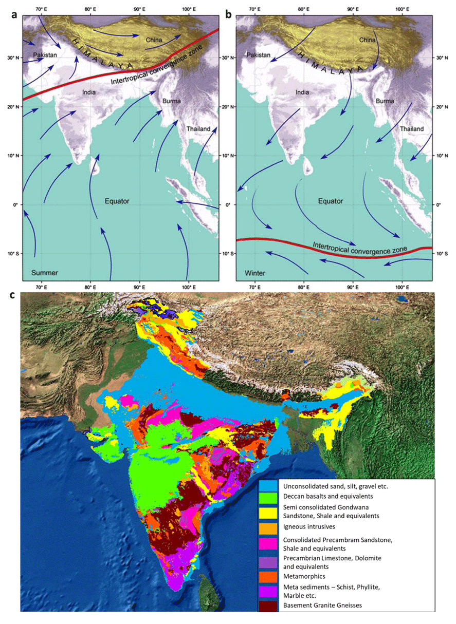
Figure 1(a) The relation between Himalayan Tibetan Plateau uplift and monsoon initiation in India. Monsoon winds blow from the Indian Ocean towards land in summer (b); during winter, the Himalayas prevent cold air from passing into the subcontinent, causing a reversal of the wind direction and for the monsoon to blow from the land toward the sea (reprinted from Chatterjee et al., 2013). Panel (c) presents the geology of Peninsular India (reprinted from the Central Ground Water Board, https://www.aims-cgwb.org/general-background.php, last access: 1 January 2024).
Peninsular India is strongly impacted by monsoons, major seasonal winds that are a manifestation of the seasonal movement of the Intertropical Convergence Zone (ICTZ in Fig. 1a and b), which contribute largely to the annual rainfall variability over much of the subcontinent (Gadgil, 2003). The monsoons have two components: the south-west monsoon and north-east monsoon, which arrive during June–September (JJAS) and October–December (OND), respectively. The south-west monsoon season contributes more than 75 % of the annual rainfall over the majority of the country (Saha et al., 1979). However, the southern region of Peninsula India receives a significant portion (30 %–60 %) of its annual rainfall during the north-east monsoon, which contributes only 11 % of the rainfall annually to India as a whole (Rajeevan et al., 2012). The maximum extent of rainfall over the southern region of Peninsula India during the north-east monsoon is due to the reversal of lower-level winds over South Asia from the south-west to the north-east during the retreating phase of the south-west monsoon (Rajeevan et al., 2012). Peninsular India displays south–north variability in the south-west monsoon, causing heavy rainfall along the Western Ghats and reduced amounts in the central and north-eastern regions (Fig. S2a in the Supplement).
The Western Ghats' long escarpment hosts predominantly tropical evergreen forest, crucial for intercepting south-west monsoon winds (Ramachandra, 2018). Ramachandra (2018) depicted a west–east vegetation gradient along the Western Ghats, transitioning from tropical evergreen to semi-evergreen and progressing from moist to dry deciduous forests towards the rain shadow region in the east. A topographic map of Peninsular India and of a selected point in the region is depicted in Fig. S1a and b, respectively. The western margin of Peninsular India, influenced by the Western Ghats, receives heavy rainfall, while the rain shadow region experiences deficient rainfall (Fig. S2c). The geological and tectonic history, coupled with monsoon climate events, has significantly shaped the present landform (Kale, 2014).
The region on the Deccan Plateau of Peninsular India shown in Fig. 2 is selected as the study area. The escarpment of the Western Ghats forms the western margin of the Deccan Plateau, which serves as the main water divide for the river systems in Peninsular India. The gentle slope from west to east causes peninsular rivers, such as the Mahanadi, Godavari, Krishna, and Cauvery (Fig. 2), to flow eastwards. Three of these rivers (the Godavari, Krishna, and Cauvery) originate from the Western Ghats, spread across the area from the Deccan Plateau, flow eastwards, and drain into the Bay of Bengal. The Mahanadi River rises in the mountains of Siwaha, bounded by the Eastern Ghats in the south and east, and drain eastwards into the Bay of Bengal. Additional details about these river basins can be found in Sect. S1. The study utilizes daily streamflow data (1965–2012) from 62 gauges across four river basins, sourced from the Water Resources Information System (WRIS) database. The analysis incorporates a daily gridded (0.25° × 0.25°) rainfall product from the India Meteorological Department (IMD; Pai et al., 2014).
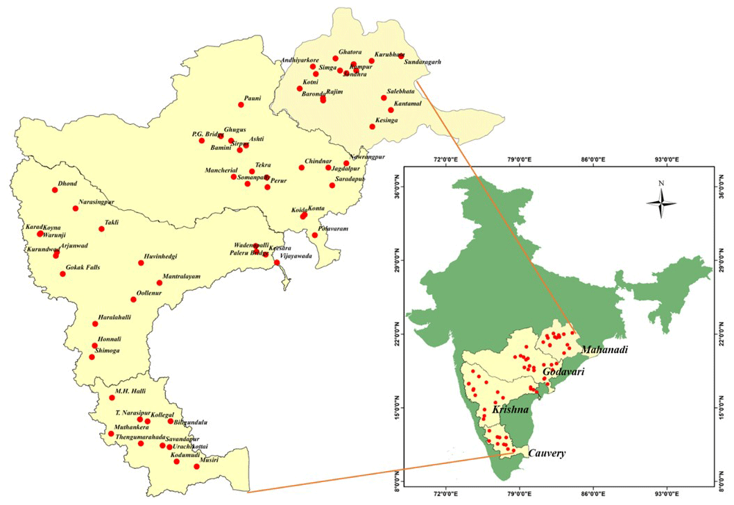
Figure 2Location map of four river basins in Peninsular India. Stream gauges considered in this study are marked with red circles.
Initially, the study employs timescale partitioning to analyse FDCs across Peninsular India, focusing on the non-monsoon, south-west monsoon, and north-east monsoon periods in four river basins. The analysis extends to regional scales, encompassing streamflow time series from all gauging stations, and includes process-scale partitioning to assess the relative contributions of fast- and slow-flow components, revealing spatial patterns influenced by climate, geology, and aquifer characteristics.
Additionally, the methodology entails a comprehensive analysis of FDCs for fast- and slow-flow components across seasons. It includes scaling time series to remove the influence of mean climate and geology and utilizing the statistical distributions to examine parameters influencing FDC shapes. The study explores links between statistical parameters and landscape properties through recession analysis and investigates spatial variation in FDC parameters using descriptors such as latitude, longitude, and catchment area. The final part of the methodology focuses the association between the midsection slope of the FDC and recession parameters, exploring the role of both surface and subsurface processes in controlling the average flow regime of the catchment.
3.1 Timescale partitioning
The streamflow hydrograph, representing a catchment's response to random rainfall events, is treated as a stochastic time series, with streamflow considered a random variable. Utilizing distribution functions like the cumulative distribution function (CDF) allows for a concise assessment of streamflow variability, aiding in the interpretation and comparison of catchment responses. CDFs have diagnostic and practical value, facilitating the classification of catchments based on flow regimes and supporting probabilistic treatments in engineering design and environmental monitoring. The CDF of a random variable (the random variable of interest to us is daily streamflow, Q) expresses the probability that a realization (i.e. observation) of Q does not exceed a specific value q.
The FDC, an equivalent measure of streamflow variability, represents the fraction of time (D) that streamflow is likely to equal or exceed a specified value, expressed mathematically as follows:
Despite its probabilistic definition, the FDC is commonly plotted in hydrological applications as q(D), i.e. q (on the vertical axis) as a function of D (on the horizontal axis).
The streamflow time series can be equivalently divided into temporal segments of distinct seasons as well as distinct months. In this case, by joining observed time series over multiple years, FDCs for each time segment can be reconstructed. Assuming independence (as an approximation), these can then be combined to generate annual FDCs. The theory for the timescale partitioning is illustrated in Fig. 3a. The year is divided into three distinct (nonoverlapping) seasons, i.e. the non-monsoon, south-west, and north-east seasons (for Peninsular India), of relative durations τ1, τ2, and τ3 (with , respectively. These seasons can be assumed to have distinct characteristics in terms of rainfall variability and how they translate to streamflow variability. The daily streamflow time series is used to construct the seasonal and annual FDCs. For example, the FDC of the non-monsoon season is constructed using the daily streamflow during the period of January–May over the years. Similarly, FDCs for the south-west and north-east monsoon seasons are constructed using the daily streamflow during the respective June–September and the October–December months over the years, whereas the annual FDC is constructed using daily streamflow values for 365 or 366 d over the years. The FDCs at monthly timescales are obtained using the daily values of streamflow in a month over the years. The FDCs for the three distinct seasons, i.e. non-monsoon, south-west monsoon, north-east monsoon seasons, are denoted as DNM(q), DSW(q), and DNE(q), respectively. Initially, the FDCs for each season can be constructed separately (Fig. 3a).
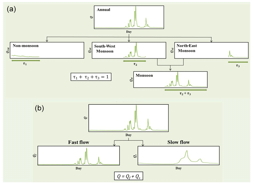
Figure 3Timescale and process-scale partitioning. (a) Scale partitioning into seasonal and monthly timescales. The conceptual framework illustrates the timescale partitioning of streamflow time series into various seasonal components considering patterns of rainfall variability. The annual streamflow time series is decomposed into three components: (1) non-monsoon flow, (2) south-west monsoon flow, and (3) north-east monsoon flow. (b) The schematic representation illustrates the process partitioning of streamflow time series into the fast-flow and slow-flow components.
The annual FDC with exceedance probability P[Q ≥q] refers to the probability of annual-scale flow being greater than or equal to q, and it is expressed as follows:
Here, P(NM)[Q ≥q], P(SW)[Q ≥q], and P(NE)[Q ≥q] refer to the probability of flow in the respective non-monsoon, south-west monsoon, and north-east monsoon seasons being greater than q. As the seasons are nonoverlapping, the probability of flow being greater than q at the annual scale (i.e. P [Q ≥q]) can be expressed as the sum of the weighted probabilities of flow being greater than q in the three seasons.
In general, the FDC at the annual scale can be constructed as follows:
where n is the number of distinct seasons considered for the analysis and . The validity of the above depends on the assumption that there is no carryover of flows from one season to the next season (which is an approximation). In this study, the assumption of independence between flows across three seasons is checked using a multivariate Hoeffding's test (see details in Sects. S2 and S3).
The relative contributions of the non-monsoon, south-west monsoon, and north-east monsoon flows to the annual flow, CNM→AN, CSW→AN, and CNE→AN, respectively, can be approximated via the following corresponding expressions:
Similarly, the relative contributions of monthly flows to annual flow can be expressed as follows:
Note, as before, these relative contributions to total flow effectively also measure the relative contributions of the seasonal or monthly flows to the mean of the annual FDC.
The methodology for constructing the annual FDC using seasonal FDCs is as follows:
-
The empirical probability density functions (PDFs) – fNM(q),fSW(q), and fNE(q) – are derived for daily streamflow time series for the non-monsoon, south-west monsoon, and north-east monsoon seasons, respectively.
-
These PDFs are then multiplied by corresponding scaling factors, τ1,τ2, and τ3, in Eq. (S4). The scaling factors represent relative durations of the three seasons considered. For example, , as the duration of the non-monsoon season is 5 months.
-
The PDF of annual flow is estimated as the weighted sum of three scaled density functions corresponding to the three seasons (see Eq. S2). The annual flow consists of the daily streamflow for the non-monsoon, south-west monsoon, and north-east monsoon seasons.
The performance of the timescale partitioning framework is assessed using the root-mean-square error (RMSE) metric. The method of estimation of qsim is shown in Fig. S3.
3.2 Process partitioning
Daily streamflow is partitioned in such a way that it approximates the statistical summation of fast flow and slow flow at the daily scale (Fig. 3b):
where Q is the daily streamflow, Qf is the daily fast flow, and Qs is the daily slow flow.
The relative contributions of fast flow and slow flow to total flow, C→ TF and CSF → TF, respectively, can be expressed as follows:
Note that and effectively measure the relative contributions of fast and slow flows to the mean of the annual FDC.
3.3 Exploring FDC controls and spatial patterns: insights from statistical distributions and analysis of midsection slope
The analysis then extends to the comprehensive analysis of FDCs for fast- and slow-flow components across different seasons, with a focus on understanding their variations and controls. The first step is to scale the fast- and slow-flow time series by their respective long-term mean values, effectively removing the influence of mean climate and geology. This scaling allows the identification of secondary controls on the shapes of FDCs.
A MGD is then used to fit the scaled fast- and slow-flow time series, and the parameters of the MGD are examined for their influence on the FDC shapes (see Sect. S4; Krasovskaia et al., 2006; Botter et al., 2007; Muller and Thompson, 2016; Santos et al., 2018). The variation in the parameters of the MGD are explored, regionally and seasonally, considering the influence of mean climate, geology, and complex hydrological processes on fast and slow flows. The performance of the MGD with respect to fitting FDCs is assessed using goodness-of-fit metrics such as the Nash–Sutcliffe efficiency (NSE) and coefficient of determination (R2). Seasonal variations in MGD parameters are analysed at a regional scale, considering all gauging stations. The studies conducted by Botter et al. (2013), Muller et al. (2014), Basso et al. (2015), Arai et al. (2021), and Leong and Yokoo (2022, 2019) illuminate the complex interplay between recession parameters and FDC characteristics, underscoring the pivotal influence of recession parameters on hydrological systems, encompassing catchment attributes and storage–discharge relationships. Consequently, in pursuit of a deeper understanding, we delve into examining the connection between MGD parameters and landscape properties via recession analysis. Spatial variation in FDC parameters is then investigated using descriptors such as latitude, longitude, and catchment area.
The final aspect of the methodology involves the association between the midsection slope of the FDC and recession parameters, emphasizing the role of both surface and subsurface processes in controlling the average flow regime of the catchment. The methodology aims to unravel the intricate interplay of climate, geology, and hydrological processes in shaping the regional hydrological signatures of Peninsular India.
4.1 Timescale partitioning
We initially investigated the spatial variations in seasonal and annual FDCs across Peninsular India employing the partitioning framework. The annual FDC and seasonal FDCs for the non-monsoon, south-west monsoon, and north-east monsoon seasons are shown in Fig. 4 for eight representative gauges: one in the upstream section and one in the downstream section of each of the four river basins. The estimated annual FDC (red curve), calculated using Eq. (S2), is also shown in Fig. 4. The daily streamflow time series is normalized by catchment area before plotting (on a semi-log scale) the FDC for comparison across the gauging stations. In particular, the annual FDC (black scatter in Fig. 4) is reproduced well by the partitioning of both seasonal (red curve in Fig. 4) and monthly flows (red curve in Fig. S4). The mean and variance of annual flows are also reproduced well by the timescale partitioning framework (Fig. S5). This confirms the efficacy of the timescale partitioning approach of seasonal or monthly flows in approximating the annual FDC (see also Figs. S4 and S5a and d).
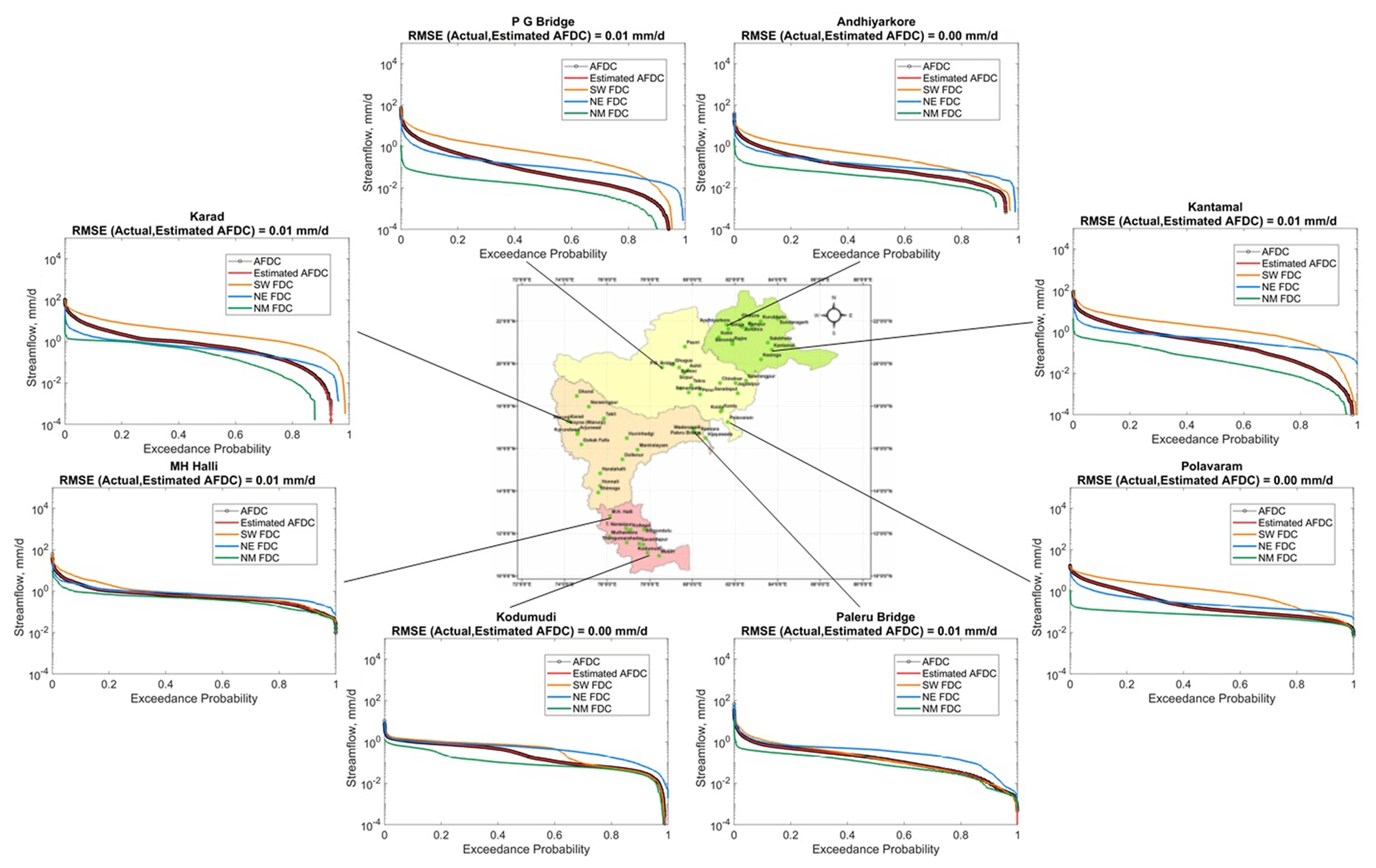
Figure 4Spatial variations in seasonal and annual FDCs across Peninsular India. The timescale partitioning framework of seasonal flows in approximating annual FDCs works reasonably well.
Another feature that can be observed in Fig. 4 is that, for gauging stations located in the northern part of the peninsular region, the FDCs of south-west monsoon flows (orange curve in Fig. 4) are relatively higher compared with other seasonal FDCs. Given the logarithmic scale used to plot the flows, this dominance is significant. At sites located in the southern part of the region, the dominance of the south-west monsoon is not as strong and north-east monsoon flows (blue curve in Fig. 4) are also significant.
Motivated by these observations, we extracted seasonal and monthly streamflow time series from the entire dataset across all gauging stations to compute the relative contributions of seasonal and monthly flows to the annual FDC. The results are presented in Fig. 5. At the monthly scale (Fig. 5a–d), the contributions of flows during the months of June–September are much higher than those in other months in northern basins (Mahanadi and Godavari as well as Krishna to a lesser extent) in Peninsular India. This can be explained by the contribution of monthly rainfall to annual rainfall, which is higher during these months, as shown in Fig. S6. On the other hand, in the southernmost Cauvery Basin, the dominance of the June–September months is not as strong, and there is also a significant contribution during the months of October–December, higher than in northern basins (Fig. 5d). This can be attributed to the slightly more equal dominance of both the south-west (June–September) and north-east (October–December) monsoons over the Cauvery Basin (Fig. S6d) compared with the northern basins. This pattern is also reflected at the seasonal scale (Fig. 5e–h), with the contribution of the south-west monsoon flow to annual flow being slightly higher than that during the other seasons and much higher in northern basins. However, the contribution of the south-west monsoon to annual flow decreases in southern basins, while the contribution of north-east monsoon increases, as can be seen clearly in Fig. 5h for the Cauvery Basin. The contribution of the non-monsoon season to annual flow is also higher in southern basins relative to the northern basins. This can be attributed to carryover flows from winter rains during the north-east monsoon, which is more pronounced in the southern part of the region.
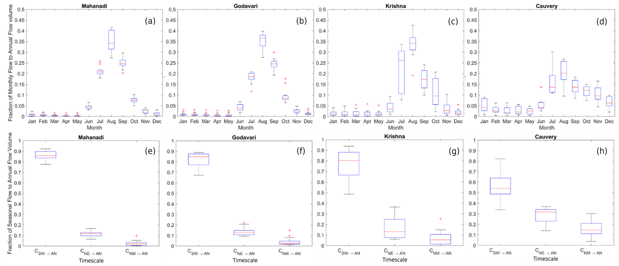
Figure 5The relative contributions of monthly and seasonal flows to annual flow at the basin scale. The contributions of south-west monsoon flow to annual flow increases in northern basins, whereas it decreases in southern basins; however, the contributions of north-east monsoon flow to annual flow increases towards southern basins.
We next carried out regional-scale analysis by considering streamflow time series of all the gauging stations across all four river basins. Similar to the basin-scale analysis presented before, the relative contributions of seasonal and monthly flows to annual flow are now estimated at the regional scale (Fig. 6). The spatial patterns of south-west and north-east monsoon rainfall across Peninsular India are plotted for comparison using the IMD gridded rainfall product (Fig. 6b, e).
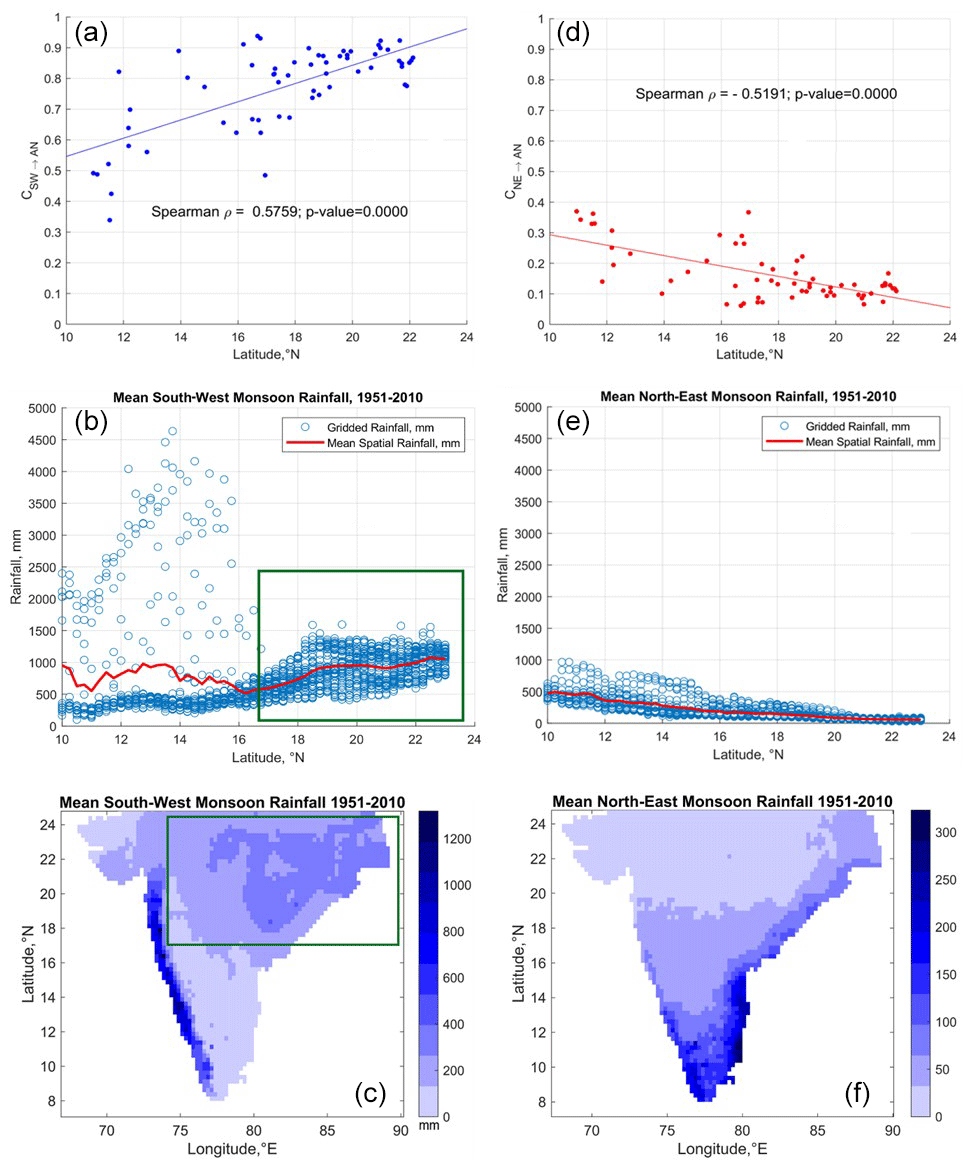
Figure 6Contribution of seasonal flows to annual flow at the regional scale. The spatial variability in the south-west (a) and north-east (d) monsoons can explain the variation in the contributions of seasonal flows to annual flow across a south–north gradient. The green box in panel (b) indicates the northern part of Peninsular India, which receives higher rainfall than the southern part. The green box in panel (c) indicates the spatial extent of the rainfall grids that were considered in panel (b). The red line in panel (b) indicates the mean rainfall, which was obtained by averaging the rainfall values at a specific latitude (° N). Decreasing mean rainfall is observed during the north-east monsoon (e, f), which corroborates the association shown in panel (d).
The contribution of south-west monsoon flows to annual flow increases in the northerly direction (Fig. 6a). The mountainous region of the southern part of Peninsula India (western part of Krishna Basin and north-western part of Cauvery Basin) receives high rainfall during the south-west monsoon season (Fig. 6b – extended until 17° N). The streamflow produced in the headwater regions of southern basins in response to high rainfall, contributes at least 70 % of the annual flow (Fig. 6a). However, the areal fraction of these high-rainfall headwater regions within the four river basins is quite small, and their contributions to the average precipitation or flow at the basin scale is much smaller. There is also considerable variability in the contributions of south-west monsoon flows to annual flow in the subbasins located in the eastern and south-eastern parts of the Krishna and Cauvery basins (represented by the scatter below the regression line until 17° N in Fig. 6a) due to declining rainfall (Fig. 6c). This considerable variability, on average, reduces the overall contributions of the south-west monsoon to annual flow in southern peninsula region with respect to the basins in the northern part.
The northern part of Peninsular India receives comparatively higher rainfall than the southern part without considering the Western Ghats. This increased rainfall is attributed to the movement of low-pressure systems that develop over the Bay of Bengal towards central India (Krishnamurthy and Ajayamohan, 2010; Prakash et al., 2015). The low-pressure systems are a regular feature of the south-west monsoon, which brings a significant amount of rainfall in the northern part of Peninsular India (Krishnamurthy and Ajayamohan, 2010). The increased rainfall (Fig. 6b – after 16° N) is responsible for the higher contribution of south-west monsoon flows to annual flow in the northern basins. As the spatial variability in this rainfall is comparatively less than in the southern peninsular region, there is less variability in the contribution of south-west monsoon flows to the annual flow. The spatial variability in the south-west monsoon along the south–north direction across the Peninsular India region can explain the gradient in the contribution of south-west monsoon flows to annual flow in the same direction.
On the other hand, the contribution of north-east monsoon flows to annual flow increases in the southerly direction (Fig. 6d, e). This can be explained by the fact that the southern part of Peninsular India receives higher rainfall during north-east monsoon than the rest of Peninsular India (Fig. 6f).
The application of the analysis framework used here is based on the critical assumption of independence of flows between different seasons (months), which needs to be critically evaluated. Moisture carryover across seasons is a confounding issue in the case of strongly seasonal catchments (i.e. exhibiting sharp transition from the wet season to the dry season in terms of rainfall climatology), specifically when the initial wetness condition at the onset of the dry season depends on the final wetness at the end of wet season and vice versa. Although most of the rainfall (58 %–90 %) is concentrated during south-west monsoon months (i.e. June–September, red bar in Fig. S7) in basins in Peninsular India, more than 10 % of the annual rainfall is received during north-east monsoon months (i.e. October–December, yellow bar for Cauvery and Krishna basins in Fig. S7). In addition, more than 8 % of annual rainfall occurs in the non-monsoon season (i.e. January–May, blue bar in Fig. S7). This highlights that rainfall received during the non-monsoon and north-east monsoon seasons are comparable; thus, it is difficult to distinguish the rainfall climatology across these seasons. It is consequently challenging to declare that these are catchments with seasonally dry climates. In order to justify our assumption in the reconstruction of the annual FDC from seasonal flows, we conducted a multivariate Hoeffding test (Gaißer et al., 2010) to check the independence between three random variables representing the non-monsoon, south-west monsoon and north-east monsoon flows, respectively. A value of the test statistic φ2 that is close to zero indicates independence between the three random variables. It is observed that, except for two stations in Krishna Basin, 60 out of 62 stations show independence between flows across the seasons (Fig. S8). This supports the appropriateness of the no-carryover assumption used in this study to construct the annual FDC based on seasonal FDCs.
4.2 Combined influence of timescale and process-scale partitioning
In order to further explore the climatic and landscape controls on streamflow variability at a regional scale, we next partitioned streamflow into fast- and slow-flow components, notionally representing surface runoff, and a combination of subsurface and groundwater flow, respectively (Ghotbi et al., 2020a, b). Fast flow is controlled by event-scale runoff generation processes and its variability is characterized by topography, land use, soil, and rainfall characteristics. On the other hand, climate seasonality and geological formations of the subsurface are primary controllers of slow-flow variability (Ghotbi et al., 2020a, b). The slow-flow component is extracted from observed streamflow using a recursive digital filter (see details in Sect. S5). The fast-flow component is obtained by then subtracting the slow flow from observed streamflow. The relative contributions of fast flow and slow flow to total flow (and, hence, also mean annual flow) are estimated using Eqs. (11) and (12), respectively, for all the gauging stations across all four basins. The relative contributions of fast and slow flows to total flow at the basin and regional scales (combining all the gauging stations) are shown in Fig. 7. In addition, the long-term mean annual rainfall across Peninsular India is also presented for comparison and to possibly explain the contributions of fast flow (Fig. 7h).
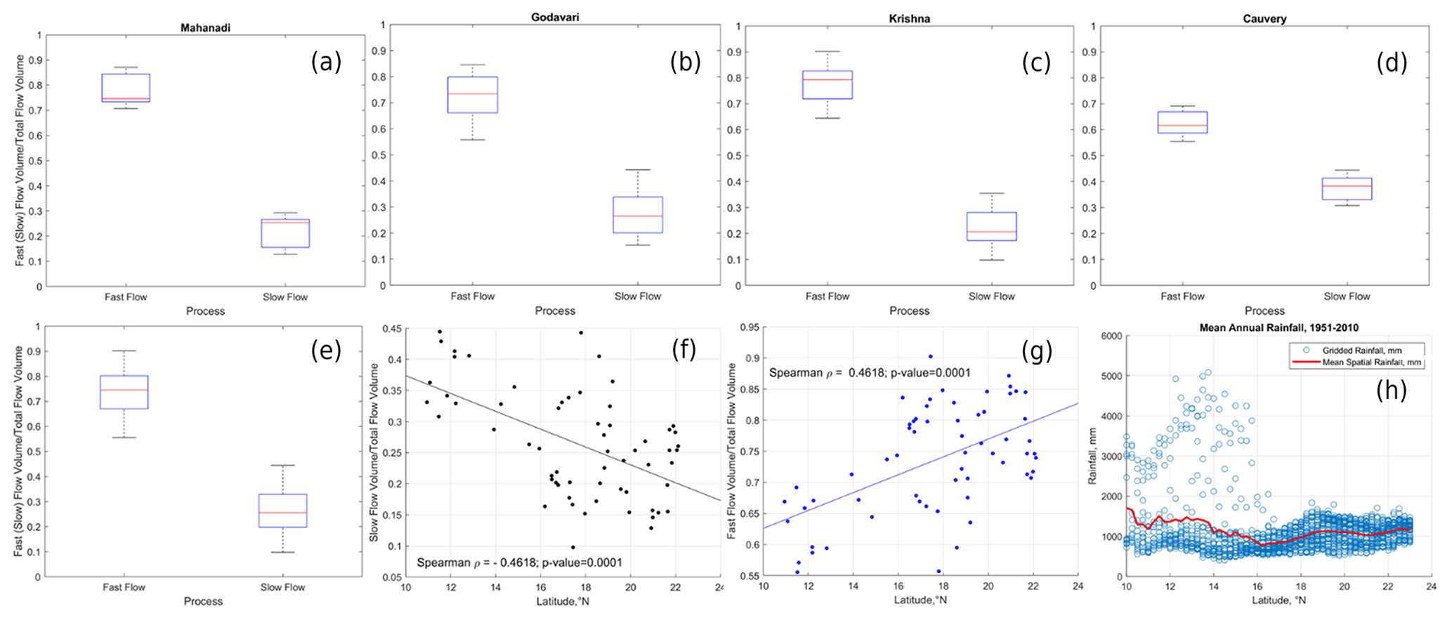
Figure 7Relative contributions of fast and slow flow to total flow. A consistently higher contribution of fast flow and a lower contribution of slow flow to total flow are observed in Peninsular India (a–d) at the basin scale. At the regional scale, a systematic gradient in the fast- and slow-flow contributions is observed (f, g). The spatial patterns of rainfall (h) can explain the gradient in fast-flow contributions. The high scatter of rainfall in the low latitudes represents the heavy rainfall with high variability occurring in the Western Ghats.
The contributions of fast and slow flows to total flow in each of the four river basins is presented in Fig. 7a–d, indicating a strong dominance of fast flow in the northern basins (close to 80 % in the Mahanadi, Godavari, and Krishna basins) and relatively less dominance (around 60 %) in the southern Cauvery Basin. This dominance of fast flow is also seen at the regional scale (Fig. 7e). The regional variations in the relative contributions of slow and fast flows to total flow can also be seen in the results for individual gauges presented in Fig. 7f and g, respectively. On average, the contribution of slow flow decreases in the northerly direction, whereas the contribution of fast flow increases in a corresponding way.
The contribution of fast flow to total flow increases in the northern direction in Peninsular India (Fig. 7g). The fast-flow component of streamflow is generally more responsive to the characteristics of rainfall intensity. The southern part of the region receives high rainfall over Western Ghats along the western edge of Krishna Basin and Cauvery Basin (Fig. 7h). In Cauvery Basin, the headwater catchments (namely, MH Halli, Muthankera, and Thengumarahada; Fig. S6) contribute 57 %–65 % of fast flow to total flow locally. The subbasins located at the western edges of Krishna Basin contribute 80 % of the fast flow to total flow (between 13 and 18° N; Fig. 7g) locally. However, there is a wide range of variability in the contributions of fast flow to total flow for subbasins located in the eastern part of Krishna Basin. The spatial mean rainfall increases and variability decreases after 16° N (Fig. 7h), dictating the increased contribution of fast flow to total flow. Therefore, the spatial characteristics (mean and variability) of annual rainfall control the south–north gradient in fast-flow contributions to total flow. In order to explain the variability in the slow-flow fraction of total flow, a multivariate regression analysis is performed (details are provided in Sect. S8). It is observed that the location of the gauges is an important predictor of the slow-flow fraction of total flow in Peninsular India, revealing the existence of a regional groundwater gradient in the region (see Sect. S7 and Table S1). In addition to the location of the gauges, the recession parameter β, which controls the aquifer geometry and water level elevation profile during early and late stages of recession, is found to be significant in explaining the slow-flow fraction of total flow (see Sect. S7 and Table S1).
The contributions of slow flow to total flow increases in a southerly direction over Peninsular India (Fig. 7f). This can be explained by two major factors. Firstly, the peninsular region is mostly dominated by hard-rock geological formations, where the subsurface flows are controlled by secondary porosities due to weathering and fracturing (Chandra, 2018; Das, 2019). The distribution of these formations is highly heterogenous (Fig. 1c) and is responsible for the baseflow (slow-flow) contribution to total flow (Collins et al., 2020; Narasimhan, 2006). For example, 84 % of the total area of Cauvery Basin is classified as moderate to good groundwater potential zones (Arulbalaji et al., 2019). The influence of such potential regions in Cauvery Basin is reflected in the presence of a significant amount of slow flow, even in the non-monsoon season (Fig. 8g, h). Likewise, 63 % of the total area of Krishna Basin is classified in the same manner (Harini et al., 2018). However, the slow-flow regime becomes much more seasonal (Fig. 8) in the northern part of Peninsular India due to the limited capability of geological formations to transmit slow flow (Patil et al., 2017) and to strong seasonality in rainfall patterns (Fig. 8). Secondly, the southern part of the peninsula receives almost equal rainfall during both the south-west and north-east monsoons, which is reflected in the bimodal pattern of rainfall seasonality (Fig. 8g, h). The compounding effect of bimodal rainfall seasonality and the higher fraction of moderate to good groundwater potential zones explains the higher contribution of slow flow to total flow in southern part of Peninsular India.
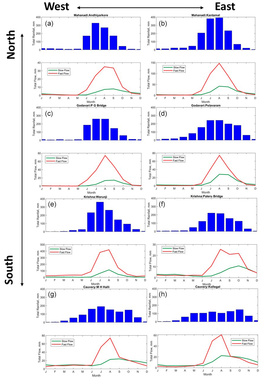
Figure 8Spatial variation in the long-term monthly fast- and slow-flow components of streamflow at selected gauges in Peninsular India. The blue bar plots represent the long-term monthly rainfall averaged over the subbasins corresponding to the gauging stations. The seasonality in rainfall pattern changes (unimodal to bimodal) across a north–south direction in Peninsular India.
Further, an investigation of the combined influence of climatic timescales and process timescales is, therefore, pertinent to fully understand the controls on streamflow variability in this region. To address this question, we extracted the fast- and slow-flow components for the respective non-monsoon, south-west monsoon, and north-east monsoon seasons. These components are then used to estimate their relative contributions to total flow for the three seasons across all of the gauging stations.
The relative contributions of fast and slow flow to total flow at the basin scale are shown in Fig. 9. It is observed that the median contributions of fast and slow flow for the Mahanadi, Krishna, and Cauvery basins are similar during the non-monsoon period, although considerable variability exists with respect to their distribution. With the onset of the south-west monsoon, the contribution of fast flow to total flow increases markedly for all of the basins, although much less in the Cauvery Basin. During the subsequent north-east monsoon season, the contribution of fast flow decreases, whereas the slow-flow contribution increases. The fluctuations in the fast-flow contributions can be explained by the onset and withdrawal of the monsoon seasons, which are major contributors to fast-flow generation. The fluctuations in the fast-flow contributions across seasons can be explained by the differences in the rainfall amount during the south-west and north-east monsoons (Fig. 6c, f). Among all four basins, the difference in the median contributions of fast and slow flow is minimum. This can be attributed to the presence of a higher fraction of moderate to good groundwater potential zones (Arulbalaji et al., 2019) that promote baseflow even in dry periods (Fig. 8g, h). The presence of a bimodal pattern in rainfall seasonality due to both the south-west and north-east monsoons minimizes the difference between the relative contributions of fast and slow flow to total flow.
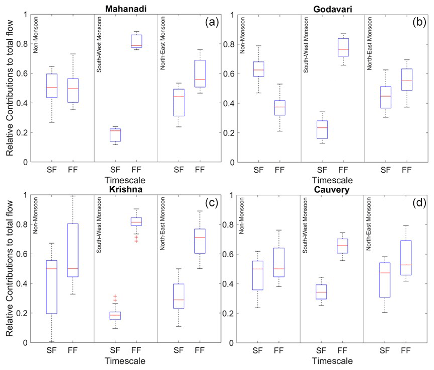
Figure 9Seasonal contributions of fast flow (FF) and slow flow (SF) to total flow at the basin scale.
5.1 Understanding physical controls on and spatial variation in the FDC by fitting statistical distributions
So far, in this paper, in order to understand the physical controls on regional streamflow variability across Peninsular India, we have partitioned observed streamflow in two ways: (i) seasonal or monthly flows and (ii) slow and fast flows. We have looked at the relative contributions of these components to mean annual streamflow, examined how the relative contributions varied regionally, and attributed these to the relative strengths of the monsoons and spatial variations in the geological formations. We now return to the FDCs of the flow components, especially the shapes of the FDCs (as reflected in the parameters of the fitted distribution) and look at how they themselves vary regionally.
In our study, the fast- and slow-flow time series are scaled by their respective long-term mean values to remove the influence of mean climate and geology, thereby providing an opportunity to identify the secondary controls on the variation in the shapes of FDCs. The scaled fast- and slow-flow time series are then used to fit the MGD (see details in Sect. S4). The parameters of the MGD control the shape and orientation of the FDC. For example, the shape parameter k controls the slope of the FDC, whereas α controls the zero-flow part of the FDC. However, the parameter θ affects the vertical shift in the FDC. In addition, these parameters are also linked to the mean and variance of the streamflow time series. For example, the scale parameter θ is directly proportional to the mean of the time series, whereas the shape parameter k is inversely proportional to the variance in the time series.
As the fast- and slow-flow time series are scaled using their respective long-term means, the scale parameter (θ) is found to be approximately inversely proportional to the shape parameter (k) via the following relationship: (Cheng et al., 2012). Therefore, the variations in only k and α (the zero-flow probability) are presented in this section. The variation in k can be related to the steepness of the FDC, i.e. smaller values of k will have steeper slopes.
The Nash–Sutcliffe efficiency (NSE) and coefficient of determination (R2) metrics outlining the goodness of fit of fast or slow flows to MGD are shown in Fig. S10. In addition, the observed and simulated FFDCs and SFDCs are compared in Fig. S8. It is observed that the slow-flow component fits well to the MGD compared with the fast-flow component, as slow flow is the most stable component and the MGD satisfactorily captured the shape of the SFDC. However, the MGD adequately captures the shape of FFDC at the upper tail (high-flow segment) but not at the lower tail (low-flow segment). The fast-flow processes are governed by more complex processes (e.g. infiltration and saturation excess runoff generation, runoff routing, the stochastic nature of storm events, and the properties of soil and topography) than slow flow (e.g. climate seasonality and the underlying geology of aquifer system).
The seasonal variation in the parameters of the MGD at the regional scale (comprising all of the gauging stations) is presented in Fig. 10. The MGD performed well with respect to fitting the FDCs of two flow components across different seasons (Fig. S10). In Fig. 10a, it is observed that the shape parameter of slow flow is consistently higher than that of fast flow. The shape parameter is inversely proportional to the variance in streamflow. The slow flow exhibits lower variance due to its longer time of residence in the subsurface formations. Moreover, the subsurface formations in Cauvery Basin are more favourable to slow flow in comparison with the other three basins (Fig. 8g, h). In addition, the bimodal seasonal pattern of rainfall is also responsible for the occurrence of slow flow, even in the non-monsoon period for the southern basins (Fig. 8).
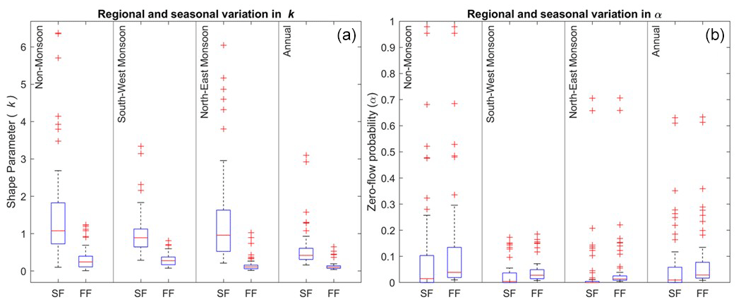
The fast-flow component exhibits higher variance than the slow-flow component. The median shape parameter of fast flow is highest during the south-west monsoon season and lowest during the north-east monsoon (Fig. 10a). This can be explained by the lower variance in fast flow during the south-west monsoon, as the rainfall amount is higher during this season compared with the north-east monsoon (Fig. 6c, f). The dominance of both the south-west and north-east monsoons in Cauvery Basin results in lower variance in fast flow compared with the northern basins. The FFDCs are steeper than the SFDCs for all seasons, as the magnitude of k for fast flow is smaller than that of slow flow (Fig. 10a).
The parameter α controls the zero-flow part of the FDC. It is observed that the mean α for slow flow is lowest during the south-west monsoon and highest during the non-monsoon season (Fig. 10b) at a regional scale. This can be attributed to the combined influence of rainfall during the south-west monsoon and the connectivity between underlying geological formations in Peninsular India. For the fast flow, the mean α is lowest during the south-west monsoon and highest during non-monsoon, as the south-west monsoon is the dominant rainfall season in Peninsular India.
The shape parameters (k) of the MGD for slow- and fast-flow components are linked with landscape properties via recession analysis, where the γ and β parameters of the power-law relationship are estimated using streamflow data (details in Sect. S6). It is observed that the shape parameter (inversely proportional to variability) of slow flow is positively correlated with β. The parameter β is influenced by the aquifer geometry and the water table elevation profile defining the early and late stages of recession (Tashie et al., 2020a, b). Higher values of β indicate slow, late recessions, which are characterized by low variability in slow flow (Fig. 11a).
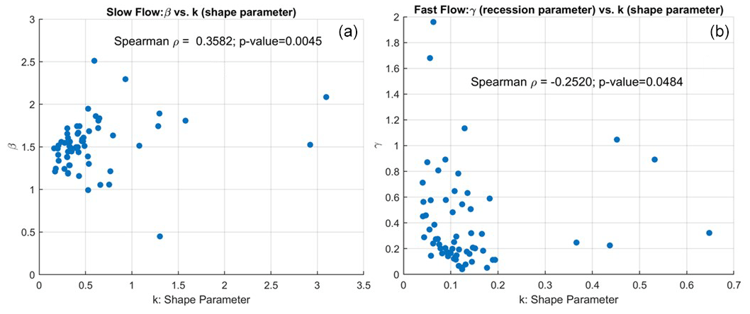
Figure 11Relationship between flow variability (related inversely to the shape parameter, k, of the MGD) and recession parameters.
The shape parameter of fast flow is negatively correlated with the parameter γ of the power-law relationship (Fig. 11b). The parameter γ is strongly related to the seasonality of catchment wetness and evapotranspiration, which are primary governing factors for runoff generation (Dralle et al., 2015; Gnann et al., 2021). In addition, the spatial variation in rainfall also influences the variability in γ (Biswal and Nagesh Kumar, 2014), which reflects the variability in fast flow.
The variation in the k and α parameters was also studied using spatial descriptors (latitude and longitude) as explanatory variables to understand the spatial variation in FDCs across south–north and west–east gradients. In addition, the behaviour of these parameters was assessed using catchment area as another explanatory variable. The regional parameter sets comprising k and α were next constructed for slow- and fast-flow processes by including these parameters for all of the time series for different gauging stations across Peninsular India. The Spearman correlation coefficients between these parameters and explanatory variables (i.e. catchment area and spatial descriptors – latitude and longitude) for slow- and fast-flow processes at seasonal scales were computed. The schematic representation of significant directions (positive or negative correlations) in the Spearman coefficients is shown in Fig. 12.
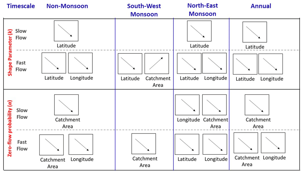
Figure 12Schematic representation of spatial and temporal variation in the MGD parameters across Peninsular India. The direction of significant Spearman correlation coefficients between model parameters and descriptors (catchment area and spatial descriptors – latitude and longitude) for fast and slow flow across multiple timescales is presented.
The shape parameter of fast flow is found to be positively correlated with catchment area (Fig. 12, top panel), implying lower variability in fast flow in large catchments. This can be attributed to the increased smoothing effect of incoming rainfall in larger catchments via various storages, thus reducing the variability in fast flow. Moreover, the shape parameters for fast flow are negatively correlated with spatial descriptors, indicating increased variability in fast flow along south–north and west–east gradients. This can be partly explained by the bimodal seasonal pattern of rainfall due to the dominance of the south-west and north-east monsoons, thus reducing the variability in fast flow in the southern part of the region. The rainfall pattern becomes more seasonal (primarily due to south-west monsoon) in the northern part of region, which can contribute to increased variability in fast flow. The presence of numerous water retention structures to support irrigation in these regions (54 %–75 % of basins in Peninsular India are cropland) can modify the variability in the flow, although we have not analysed this separately in this study.
The shape parameter of slow flow is found to be negatively correlated with latitude, implying that slow flow becomes highly variable in the northern part of the region. This can be explained by the nature of geological formations in the Cauvery Basin that promotes slow flow even during the non-monsoon period. However, in the northern part of the region, slow flow tends to become more seasonal and has very limited flow during non-rainy seasons. In addition to the geology, the bimodal seasonal rainfall patterns due to monsoons can play an important role in the variability in slow flow. Apart from the spatial descriptors, slow-flow variability is inversely proportional to catchment area, implying that larger catchments have lower slow-flow variability than smaller catchments. This can be explained by the proportional increase in the area of contribution to slow flow with increase in catchment size, thus reducing the variability in slow flow for larger catchments.
The α parameter is found to be negatively correlated with catchment area (Fig. 12, bottom panel) for fast and slow processes, implying that zero-flow probabilities are lower for larger catchments. The higher residence time of water in larger catchment due to various kinds of storage facilitates flow in rivers, even in the non-monsoon season, thereby reducing the zero-flow probabilities. In addition, the α parameter of both slow and fast flow is negatively correlated with longitude, implying lower zero-flow probabilities along a west–east direction. This can be attributed to the natural declining elevation (Fig. S1b) which promotes both fast and slow flow in an eastward direction.
5.2 Understanding physical controls and spatial variation in the seasonal FDC using the midsection slope
Apart from the mean, variance, and no-flow frequency, the midsection slope of the FDC – estimated using , where Q33p and Q66p represent the streamflow values at the respective 33rd and 66th percentiles – is connected to the average flow regime of the catchment, which is controlled by both surface and subsurface processes (Yokoo and Sivapalan, 2011; Chouaib et al., 2018). The association of the slope of the FDC with the parameters pertaining to recession analysis is presented in Fig. 13.
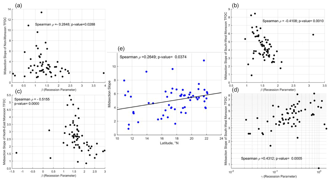
During the non-monsoon and north-east monsoon seasons (Fig. 13a, c) – when rainfall is comparatively lower than during the south-west monsoon – a significant association between flow variability and β highlights the importance of slow-flow and recession characteristics controlled by the aquifer geometry and water table elevation profile. In addition to a significant association with β during the south-west monsoon (Fig. 13b), the midsection slope of the FDC is positively correlated with γ (the parameter that is strongly related to the seasonality of catchment wetness, evapotranspiration, and spatial variation in rainfall), revealing the importance of land surface processes in streamflow variability.
A coherent pattern in streamflow variability (via the midsection slope of the FDC) is observed across a south–north gradient in Peninsular India (Fig. 13e). This systematic pattern in streamflow variability reflects the influence of the combined functioning of subsurface and land surface processes on regional hydrological signatures in this region.
The comprehensive analysis of spatial variations in seasonal and annual FDCs across Peninsular India has provided valuable insights into the controls on streamflow variability at different scales. The partitioning framework employed in this study effectively approximated annual FDCs, confirming their efficacy in capturing the intricate dynamics of seasonal and monthly flows. Noteworthy spatial patterns emerged, with gauging stations in the northern part of the peninsula exhibiting higher dominance of south-west monsoon flows in contrast to the more balanced contributions observed in the southern regions, where north-east monsoon flows also played a significant role.
The regional-scale analysis unveiled the influence of spatial patterns of monsoon rainfall, showing increased contributions of south-west monsoon flows in the northerly direction and elevated contributions of north-east monsoon flows in the southerly direction. The study also delved into the partitioning of streamflow into fast and slow components, revealing a dominance of fast flow in northern basins and an increasing contribution of slow flow in the southerly direction. Factors such as rainfall intensity, geological formations, and groundwater gradients were identified as critical controls shaping these flow characteristics. The investigation of combined influences of climatic timescales and process timescales further enriched our understanding of streamflow variability. Seasonal fluctuations in fast- and slow-flow contributions highlighted the dynamic nature of the streamflow response to monsoon onset and withdrawal. The study emphasized the importance of considering both climatic and landscape factors across different scales to comprehensively grasp the controls on streamflow variability in Peninsular India.
By undertaking an extensive analysis of FDCs for both fast- and slow-flow components across different seasons, the study aims to understand the variations and controls governing these hydrological patterns. The initial step of scaling the fast- and slow-flow time series by their respective long-term mean values serves as a crucial tool in isolating secondary controls on FDC shapes, effectively removing the influence of mean climate and geology. The subsequent use of the MGD to fit the scaled time series allows for an advanced examination of the parameters influencing FDC shapes, with a focus on the key factors of the shape parameter (k) and the probability of zero flows (α). The seasonal variations in the MGD parameters at a regional scale reveal the impact of monsoons on streamflow characteristics. Notably, the consistently higher shape parameters for slow flow highlight the lower variance attributed to longer residence times in subsurface formations, emphasizing the influence of geological features.
Further exploration into the relationships between the MGD parameters and landscape properties via recession analysis enhances our understanding of hydrological controls. The positive correlation between the shape parameter of slow flow and recession parameter β, influenced by aquifer geometry, contrasts with the negative correlation between the shape parameter of fast flow and the parameter γ, associated with the seasonality of catchment wetness and evapotranspiration. Spatial variation analysis using descriptors like latitude, longitude, and catchment area unveils significant correlations, offering insights into the influence of geographical factors on FDC shapes. The correlation of fast-flow shape parameters with catchment area suggests reduced variability in larger catchments, whereas the negative correlation of slow-flow shape parameters with latitude indicates increased variability in the northern part of the region. The examination of zero-flow probabilities controlled by the parameter α reveals noteworthy trends: larger catchments exhibit lower zero-flow probabilities, and the negative correlation of α with longitude highlights the spatial influence along the west–east direction. Finally, the study explores the midsection slope of the FDC, connecting it to average flow regimes controlled by both surface and subsurface processes. Associations with recession analysis parameters underline the integrated influence of aquifer geometry and land surface processes on streamflow variability across Peninsular India.
In summary, the methodology employed in this study offers a systematic and insightful approach to unravelling the complexities of streamflow variability across Peninsular India. This study not only enhances our understanding of the relative contributions and shapes of FDCs but also sheds light on the intricate interplay of geological, spatial, and hydrological factors influencing streamflow variability in this region.
We acknowledge, however, that streamflow variability in Peninsular India has recently been significantly impacted by anthropogenic activities, including significant land use and land cover changes as well as other human interferences such as the building of dams and the extraction of water from both rivers and groundwater aquifers for human use. The present study has not explored the effects of human impacts: their impacts on both temporal (inter-decadal) and spatial (regional) variations in the FDCs is left for future work. Further work is also needed to understand in more detail the causes and the relative contributions of regional precipitation patterns and geological formations on streamflow partitioning.
On the methodological front, there is the opportunity to refine the analysis used here to incorporate the statistical cross-correlation between fast and slow flows in the reconstruction of the FDC for total streamflow, by adopting generalized approaches (e.g. copulas). In the exploration of the relative contributions of the monsoons, there is scope to extend the analysis framework to partition the streamflow variability guided by the actual breakdown into the seasons each year in a more flexible way, as opposed to a static way. This is likely to make the results of the analysis more robust and less uncertain. Finally, in the process domain, the filter-based separation of total streamflow into fast and slow flow can be variably impacted by catchment size, introducing some uncertainty into the partitioning of the FDC of total streamflow into its fast-flow and slow-flow components. Future work in this area should explore ways to overcome these methodological shortcomings.
The streamflow datasets used for the analysis are available from https://indiawris.gov.in/wris (IWRIS, 2023). The daily IMD gridded rainfall product at a spatial resolution of 0.25° × 0.25° (https://www.imdpune.gov.in/cmpg/Griddata/Rainfall_25_NetCDF.html) from Pai et al. (2014) was used in this work. The baseflow function used for partitioning total flow to slow flow was downloaded from https://in.mathworks.com/matlabcentral/fileexchange/58525-baseflow-filter-using-the-recursive-digital-filter-technique (Qiao, 2024).
The supplement related to this article is available online at: https://doi.org/10.5194/hess-28-1493-2024-supplement.
PD, JM, and MS conceptualized the work; developed the methodology; and carried out the data curation, formal analysis, validation, and writing of the original draft. MS and PPM reviewed the initial manuscript. PPM provided the resources needed for this work.
The contact author has declared that none of the authors has any competing interests.
Publisher’s note: Copernicus Publications remains neutral with regard to jurisdictional claims made in the text, published maps, institutional affiliations, or any other geographical representation in this paper. While Copernicus Publications makes every effort to include appropriate place names, the final responsibility lies with the authors.
Pankaj Dey acknowledges a DST INSPIRE Faculty Fellowship (DST/INSPIRE/04/2022/001952, faculty reference no. IFA22-EAS 114), received from the Department of Science and Technology, Government of India, in the Earth and Atmospheric Sciences Division of 2022 call. Murugesu Sivapalan acknowledges a Satish Dhawan Endowed Visiting Professorship that enabled him to visit the Interdisciplinary Centre for Water Research (ICWaR) at the Indian Institute of Science, permitting him to participate in the research activity that culminated in this paper. Murugesu Sivapalan also acknowledges the generous support and facilities provided by ICWaR that made his stay a very productive one.
This research has been supported by the Ministry of Earth Sciences (grant no. MOES/PAMC/H&C/41/2013-PC-II); the Science and Engineering Research Board (grant no. JCB/2018/000031); and the Department of Science and Technology, Ministry of Science and Technology, India (grant no. DST/INSPIRE/04/2022/001952).
This paper was edited by Alberto Guadagnini and reviewed by Chris Leong and two anonymous referees.
Arai, R., Toyoda, Y., and Kazama, S.: Runoff recession features in an analytical probabilistic streamflow model, J. Hydrol., 597, 125745, https://doi.org/10.1016/j.jhydrol.2020.125745, 2021.
Arulbalaji, P., Sreelash, K., Maya, K., and Padmalal, D.: Hydrological assessment of groundwater potential zones of Cauvery River Basin, India: a geospatial approach, Environ. Earth Sci., 78, 1–21, https://doi.org/10.1007/s12665-019-8673-6, 2019.
Basso, S. and Botter, G.: Streamflow variability and optimal capacity of run-of-river hydropower plants, Water Resour. Res., 48, 1–13, https://doi.org/10.1029/2012WR012017, 2012.
Basso, S., Schirmer, M., and Botter, G.: On the emergence of heavy-tailed streamflow distributions, Adv. Water Resour., 82, 98–105, 2015.
Biswal, B. and Nagesh Kumar, D.: Study of dynamic behaviour of recession curves, Hydrol. Process., 28, 784–792, https://doi.org/10.1002/hyp.9604, 2014.
Botter, G., Zanardo, S., Porporato, A., Rodriguez-Iturbe, I., and Rinaldo, A.: Ecohydrological model of flow duration curves and annual minima, Water Resour. Res., 44, 1–12, https://doi.org/10.1029/2008WR006814, 2008.
Botter, G., Basso, S., Rodriguez-Iturbe, I., and Rinaldo, A.: Resilience of river flow regimes, P. Natl. Acad. Sci. USA, 110, 12925–12930, 2013.
Carlier, C., Wirth, S. B., Cochand, F., Hunkeler, D., and Brunner, P.: Geology controls streamflow dynamics, J. Hydrol., 566, 756–769, 2018.
Chandra, P. C.: Groundwater of Hard Rock Aquifers of India, CRC Press, Taylor & Francis Group, 61–84, https://doi.org/10.1007/978-981-10-3889-1_5, 2018.
Chatterjee, S., Goswami, A., and Scotese, C. R.: The longest voyage: Tectonic, magmatic, and paleoclimatic evolution of the Indian plate during its northward flight from Gondwana to Asia, Gondwana Res., 23, 238–267, https://doi.org/10.1016/j.gr.2012.07.001, 2013.
Chatterjee, S., Scotese, C. R., and Bajpai, S.: The Restless Indian plate and its epic voyage from Gondwana to Asia: Its tectonic, paleoclimatic, and paleobiogeographic evolution, Spec. Pap. Geol. Soc. Am., 529, 1–147, https://doi.org/10.1130/SPE529, 2017.
Cheng, L., Yaeger, M., Viglione, A., Coopersmith, E., Ye, S., and Sivapalan, M.: Exploring the physical controls of regional patterns of flow duration curves – Part 1: Insights from statistical analyses, Hydrol. Earth Syst. Sci., 16, 4435–4446, https://doi.org/10.5194/hess-16-4435-2012, 2012.
Chouaib, W., Caldwell, P. V., and Alila, Y.: Regional variation of flow duration curves in the eastern United States: Process-based analyses of the interaction between climate and landscape properties, J. Hydrol., 559, 327–346, https://doi.org/10.1016/j.jhydrol.2018.01.037, 2018.
Collins, L. S., Loveless, S. E., Muddu, S., Buvaneshwari, S., Palamakumbura, R. N., Krabbendam, M., Lapworth, D. J., Jackson, C. R., Gooddy, D. C., Nara, S. N. V., Chattopadhyay, S., and MacDonald, A. M.: Groundwater connectivity of a sheared gneiss aquifer in the Cauvery River basin, India, Hydrogeol. J., 28, 1371–1388, https://doi.org/10.1007/s10040-020-02140-y, 2020.
Das, S.: Frontiers of Hard Rock Hydrogeology in India, in: Ground Water Development – Issues and Sustainable Solutions, Springer Singapore, Singapore, 35–68, https://doi.org/10.1007/978-981-13-1771-2_3, 2019.
Deshpande, N. R., Kothawale, D. R., and Kulkarni, A.: Changes in climate extremes over major river basins of India, Int. J. Climatol., 36, 4548–4559, https://doi.org/10.1002/joc.4651, 2016.
Dralle, D., Karst, N., and Thompson, S. E.: a, b careful: The challenge of scale invariance for comparative analyses in power law models of the streamflow recession, Geophys. Res. Lett., 42, 9285–9293, https://doi.org/10.1002/2015GL066007, 2015.
Durighetto, N., Mariotto, V., Zanetti, F., McGuire, K. J., Mendicino, G., Senatore, A., and Botter, G.: Probabilistic description of streamflow and active length regimes in rivers, Water Resour. Res., 58, e2021WR031344, https://doi.org/10.1029/2021WR031344, 2022.
Fenicia, F., Kavetski, D., Savenije, H. H., Clark, M. P., Schoups, G., Pfister, L., and Freer, J.: Catchment properties, function, and conceptual model representation: is there a correspondence?, Hydrol. Process., 28, 2451–2467, 2014.
Gadgil, S.: The Indian Monsoon and Its Variability, Annu. Rev. Earth Pl. Sc., 31, 429–467, https://doi.org/10.1146/annurev.earth.31.100901.141251, 2003.
Gaißer, S., Ruppert, M., and Schmid, F.: A multivariate version of Hoeffding’s Phi-Square, J. Multivariate Anal., 101, 2571–2586, https://doi.org/10.1016/j.jmva.2010.07.006, 2010.
Ghotbi, S., Wang, D., Singh, A., Blöschl, G., and Sivapalan, M.: A New Framework for Exploring Process Controls of Flow Duration Curves, Water Resour. Res., 56, e2019WR026083, https://doi.org/10.1029/2019WR026083, 2020a.
Ghotbi, S., Wang, D., Singh, A., Mayo, T., and Sivapalan, M.: Climate and Landscape Controls of Regional Patterns of Flow Duration Curves Across the Continental United States: Statistical Approach, Water Resour. Res., 56, e2020WR028041, https://doi.org/10.1029/2020WR028041, 2020b.
Gnann, S. J., McMillan, H. K., Woods, R. A., and Howden, N. J. K.: Including Regional Knowledge Improves Baseflow Signature Predictions in Large Sample Hydrology, Water Resour. Res., 57, e2020WR028354, https://doi.org/10.1029/2020WR028354, 2021.
Harini, P., Sahadevan, D. K., Das, I. C., Manikyamba, C., Durgaprasad, M., and Nandan, M. J.: Regional Groundwater Assessment of Krishna River Basin Using Integrated GIS Approach, J. Indian Soc. Remote, 46, 1365–1377, https://doi.org/10.1007/s12524-018-0780-4, 2018.
IWRIS: https://indiawris.gov.in/wris, last access: 31 December 2023.
Kale, V. S., Hire, P., and Baker, V. R.: Flood Hydrology and Geomorphology of Monsoon-dominated Rivers: The Indian Peninsula, Water Int., 22, 259–265, https://doi.org/10.1080/02508069708686717, 1997.
Kale, V. S., Vaidyanadhan, R.: Landscapes and Landforms of India, edited by: Kale, V. S., Springer Netherlands, Dordrecht, 105–113 pp., https://doi.org/10.1007/978-94-017-8029-2_6, 2014.
Krishnamurthy, V. and Ajayamohan, R. S.: Composite Structure of Monsoon Low Pressure Systems and Its Relation to Indian Rainfall, J. Climate, 23, 4285–4305, https://doi.org/10.1175/2010JCLI2953.1, 2010.
Krasovskaia, I., Gottschalk, L., Leblois, E., and Pacheco, A.: Regionalization of flow duration curves. Climate variability and change: hydrological impacts, 105–110, https://www.cabidigitallibrary.org/doi/full/10.5555/20073200839 (last access: 25 October 2023), 2006.
Leong, C. and Yokoo, Y.: An interpretation of the relationship between dominant rainfall-runoff processes and the shape of flow duration curve by using data-based modeling approach, Hydrol. Res. Lett., 13, 62–68, 2019.
Leong, C. and Yokoo, Y.: A multiple hydrograph separation technique for identifying hydrological model structures and an interpretation of dominant process controls on flow duration curves, Hydrol. Process., 36, e14569, https://doi.org/10.1002/hyp.14569, 2022.
Muller, M. F., Dralle, D. N., and Thompson, S. E.: Analytical model for flow duration curves in seasonally dryclimates, Water Resour. Res., 50, 5510–5531, https://doi.org/10.1002/2014WR015301, 2014.
Müller, M. F. and Thompson, S. E.: Comparing statistical and process-based flow duration curve models in ungauged basins and changing rain regimes, Hydrol. Earth Syst. Sci., 20, 669–683, https://doi.org/10.5194/hess-20-669-2016, 2016.
Narasimhan, T. N.: Ground Water in Hard-Rock Areas of Peninsular India: Challenges of Utilization, Ground Water, 44, 130–133, https://doi.org/10.1111/j.1745-6584.2005.00167.x, 2006.
Pai, D. S., Sridhar, L., Rajeevan, M., Sreejith, O. P., Satbhai, N. S., and Mukhopadhyay, B.: Development of a new high spatial resolution (0.25° × 0.25°) long period (1901–2010) daily gridded rainfall data set over India and its comparison with existing data sets over the region, Mausam, 1, 1–18, https://doi.org/10.54302/mausam.v65i1.851, 2014 (data available at: https://www.imdpune.gov.in/cmpg/Griddata/Rainfall_25_NetCDF.html).
Patil, S., Kulkarni, H., Bhave, N., Development, W. R., Forum, P., Dialogue, P., and Conflicts, W.: Groundwater in the Mahanadi River Basin, Forum for Policy Dialogue on Water Conflicts in India, Pune, https://doi.org/10.13140/RG.2.2.11561.95846, 2017.
Prakash, S., Mitra, A. K., and Pai, D. S.: Comparing two high-resolution gauge-adjusted multisatellite rainfall products over India for the southwest monsoon period, Meteorol. Appl., 22, 679–688, https://doi.org/10.1002/met.1502, 2015.
Qiao, L.: Baseflow filter using the recursive digital filter technique, MATLAB Central File Exchange [data set], https://in.mathworks.com/matlabcentral/fileexchange/58525-baseflow-filter-using-the-recursive-digital-filter-technique, last access: 25 March 2024.
Rajeevan, M., Unnikrishnan, C. K., Bhate, J., Niranjan Kumar, K., and Sreekala, P. P.: Northeast monsoon over India: variability and prediction, Meteorol. Appl., 19, 226–236, https://doi.org/10.1002/met.1322, 2012.
Ramachandra, T. V.: Global Biodiversity Hotspot – Western Ghats: Water Tower of Peninsular India and Precious Heritage for Posterity, Centre for Ecological Sciences, Indian Institute of Science, Bangalore, https://wgbis.ces.iisc.ac.in/energy/water/paper/Peninsular%20india/dh_AUG2018_IISc_TVR_WESTERNGHATS_R.pdf, (last access: 25 March 2024), 2018.
Rehana, S. and Mujumdar, P. P.: River water quality response under hypothetical climate change scenarios in Tunga-Bhadra river, India, Hydrol. Process., 25, 3373–3386, https://doi.org/10.1002/hyp.8057, 2011.
Rehana, S. and Mujumdar, P. P.: Climate change induced risk in water quality control problems, J. Hydrol., 444–445, 63–77, https://doi.org/10.1016/j.jhydrol.2012.03.042, 2012.
Richards, F. D., Hoggard, M. J., and White, N. J.: Cenozoic epeirogeny of the Indian peninsula, Geochem. Geophy. Geosy., 17, 4920–4954, https://doi.org/10.1002/2016GC006545, 2016.
Saha, K. R., Mooley, D. A., and Saha, S.: The Indian monsoon and its economic impact, GeoJournal, 3, 171–178, https://doi.org/10.1007/BF00257706, 1979.
Santos, A. C., Portela, M. M., Rinaldo, A., and Schaefli, B.: Analytical flow duration curves for summer streamflow in Switzerland, Hydrol. Earth Syst. Sci., 22, 2377–2389, https://doi.org/10.5194/hess-22-2377-2018, 2018.
Searcy, J. K.: Flowduration curves, Man. Hydrol. U.S. Geol. Surv., https://doi.org/10.3133/wsp1542A, 1959.
Sinha, J., Sharma, A., Khan, M., and Goyal, M. K.: Assessment of the impacts of climatic variability and anthropogenic stress on hydrologic resilience to warming shifts in Peninsular India, Sci. Rep., 8, 13833, https://doi.org/10.1038/s41598-018-32091-0, 2018.
Smakhtin, V. U.: Smakhtin 2010 – Low flow hydrology.pdf, J. Hydrol., 240, 147–186, https://doi.org/10.1016/S0022-1694(00)00340-1, 2001.
Smakhtin, V. and Anputhas, M.: An assessment of environmental flow requirements of Indian river basins, IWMI Research Reports H039610, International Water Management Institute, https://publications.iwmi.org/pdf/H042045.pdf (last access: 25 March 2024), 2006.
Stewart, M. K.: Promising new baseflow separation and recession analysis methods applied to streamflow at Glendhu Catchment, New Zealand, Hydrol. Earth Syst. Sci., 19, 2587–2603, https://doi.org/10.5194/hess-19-2587-2015, 2015.
Tashie, A., Pavelsky, T., and Band, L. E.: An Empirical Reevaluation of Streamflow Recession Analysis at the Continental Scale, Water Resour. Res., 56, e2019WR025448, https://doi.org/10.1029/2019WR025448, 2020a.
Tashie, A., Pavelsky, T., and Emanuel, R. E.: Spatial and Temporal Patterns in Baseflow Recession in the Continental United States, Water Resour. Res., 56, e2019WR026425, https://doi.org/10.1029/2019WR026425, 2020b.
Vogel, R. M. and Fennessey, N. M.: Flow-Duration Curves. I: New Interpretation and Confidence Intervals, J. Water Resour. Plan. Manag., 120, 485–504, https://doi.org/10.1061/(ASCE)0733-9496(1994)120:4(485), 1994.
Vogel, R. M. and Fennessey, N. M.: Flow Duration Curves Ii: a Review of Applications in Water Resources Planning, J. Am. Water Resour. As., 31, 1029–1039, https://doi.org/10.1111/j.1752-1688.1995.tb03419.x, 1995.
Wagener, T., Blöschl, G., Goodrich, D. C., Gupta, H. V., Sivapalan, M., Tachikawa, Y., Troch, P. A., and Weiler, M.: A synthesis framework for runoff prediction in ungauged basins, in: Runoff Prediction in Ungauged Basins, Cambridge University Press, 11–28, https://doi.org/10.1017/CBO9781139235761.005, 2013.
Ye, S., Yaeger, M., Coopersmith, E., Cheng, L., and Sivapalan, M.: Exploring the physical controls of regional patterns of flow duration curves – Part 2: Role of seasonality, the regime curve, and associated process controls, Hydrol. Earth Syst. Sci., 16, 4447–4465, https://doi.org/10.5194/hess-16-4447-2012, 2012.
Yokoo, Y. and Sivapalan, M.: Towards reconstruction of the flow duration curve: development of a conceptual framework with a physical basis, Hydrol. Earth Syst. Sci., 15, 2805–2819, https://doi.org/10.5194/hess-15-2805-2011, 2011.