Technical note: Testing the connection between hillslope-scale runoff fluctuations and streamflow hydrographs at the outlet of large river basins

A series of numerical experiments were conducted to test the connection between streamflow hydrographs at the outlet of large watersheds and the time series of hillslope-scale runoff yield. We used a distributed hydrological routing model that discretizes a large watershed (∼ 17 000 km²) into small hillslope units (∼ 0.1 km²) and applied distinct surface runoff time series to each unit that deliver the same volume of water into the river network. The numerical simulations show that distinct runoff delivery time series at the hillslope scale result in indistinguishable streamflow hydrographs at large scales. This limitation is imposed by space-time averaging of input flows into the river network that are draining the landscape. The results of the simulations presented in this paper show that, under very general conditions of streamflow routing (i.e., nonlinear variable velocities in space and time), the streamflow hydrographs at the outlet of basins with Horton–Strahler (H–S) order 5 or above (larger than 100 km² in our setup) contain very little information about the temporal variability of runoff production at the hillslope scale and therefore the processes from which they originate. In addition, our results indicate that the rate of convergence to a common hydrograph shape at larger scales (above H–S order 5) is directly proportional to how different the input signals are to each other at the hillslope scale. We conclude that the ability of a hydrological model to replicate outlet hydrographs does not imply that a correct and meaningful description of small-scale rainfall–runoff processes has been provided. Furthermore, our results provide context for other studies that demonstrate how the physics of runoff generation cannot be inferred from output signals in commonly used hydrological models.

1 Introduction

The question of how will river flows change in the presence of climatic and anthropogenic changes dominates the literature in water resources journals and research conducted around the world (Arnell and Lloyd-Hughes, 2014; Blöschl et al., 2019; Gudmundsson et al., 2021; Hirabayashi et al., 2013; Whitehead et al., 2018). Slowly evolving regional climatic changes and rapid anthropogenic modifications to the landscape will impact how watersheds deliver water to communities along the river network, and recognition of this fact has fostered the development of methods and techniques to address this urgent problem (Kang et al., 2016; Kourtis and Tsihrintzis, 2021). Physics-based hydrological modeling has emerged as the preferred alternative for predicting the future of the hydrological cycle under the projected changes (Barnett et al., 2008). An example of rapid anthropogenic change in the US Midwest is the use of drainage tiling, which is effective for increasing corn yields by promoting the rapid movement of subsurface flows into rivers (Fonley et al., 2021; Schilling et al., 2019; Schilling and Helmers, 2008; Velásquez et al., 2021). This raises the question of how these landscape modifications will impact the cycles of flooding and droughts in future climatic scenarios (Akter et al., 2018; Júnior et al., 2015; Peng et al., 2019). In the typical approach to this question, a land-surface model is conceptualized, calibrated, validated, and then forced with past and future climatic inputs (rainfall, radiation, relative humidity) derived from global circulation models (Barnett et al., 2008; Condon et al., 2015; Hidalgo et al., 2009; Sadeghi Loyeh and Massah Bavani, 2021; Taye et al., 2015; Quintero et al. 2018). The underlying premise is that the hillslope-scale process equations correctly describe the water movement and partitioning into runoff and infiltration. This premise allows for changing parameter values to reflect future land-surface conditions (e.g., vegetation types, deforestation, land cover, land use) along with future conditions of meteorological forcing. Nevertheless, results from Huang et al. (2017) at 12 large-scale watersheds using nine models indicate significant limitations during extreme events. Some limitations can be improved by calibration at the cost of losing representation of processes such as evapotranspiration (Ahmed et al., 2023).

The use of land-surface models relies on their validation after parameter calibration (Beven, 1989). Historically, parameters in land-surface models are adjusted (calibrated) to match streamflow hydrographs at gauged sites in the outlet of large watersheds (> 100 km²), and a portion of the data is left to validate the hydrological model using unobserved events (Bérubé et al., 2022; Gupta et al., 2006; Refsgaard, 1997; Shen et al., 2022). Once this test has been passed, a land-surface model is deemed appropriate to explore future scenarios (Sadeghi Loyeh and Massah Bavani, 2021; Schilling et al., 2008; Whitehead et al., 2018). Several authors have highlighted the issue that stronger and more appropriate methods and techniques for validating/invalidating hydrologic models are needed (e.g., Beven and Lane, 2019), but the ability to simulate streamflow hydrographs continues to dominate the literature as the standard for model validation. Other data-based techniques for streamflow prediction are not appropriate to address these questions, because their parameters cannot be directly linked to physical processes and because there is a recognition that non-stationarities render historical information unreliable to predict the future behavior of hydrological systems (Bayazit, 2015; Cancelliere, 2017; Milly et al., 2008; Salas et al., 2018). Furthermore, a recent simulation-based study by Remmers et al. (2020) concluded that “it is challenging and in most cases impossible to infer model structure from model output for the part of model space, bucket-based hydrological models, that [were] sampled”. This again raises the historic question: what are the mechanisms that blur such differences? This issue of identifiability of hydrologic models has been raised as far back as research in the early 60s (Dawdy and O'Donnell, 1965). In this sense, different authors have arrived at similar conclusions. According to de Boer-Euser et al. (2017), it is challenging to link hydrograph differences and model structure components. Moreover, in an intercomparison experiment of three models, Vetter et al. (2015) observed similar performance among them. Tijerina et al. (2021) described similar spatial performance of two hydrological models over the conterminous USA and the Mai et al. (2022) comparison of 13 models obtained different rankings in the best-performing models when evaluating discharge versus distributed variables such as snow-water equivalent (SWE). Additionally, in the recent evaluation of the Hydrology Laboratory Research Distributed Hydrologic Model (HL-RDHM) by Madsen et al. (2020), it was shown that the performance of streamflow predictions was scale dependent, decreasing for small basins compared to the performance in larger basins, a result that is consistent with other multiscale evaluations of predictive performance of distributed models (Seo et al., 2021, 2023).

There is a long history in the hydrologic literature showing that dispersion and aggregation of flows in the river network dominates the shape of the hydrograph at larger scales (Surkan, 1968; Kirkby, 1976; Beven and Wood, 1993; Snell and Sivapalan, 1994; Mantilla et al., 2006; Zarlenga et al., 2022); however, there is not a systematic evaluation of how quickly the river network effects dominate over hillslope-scale variability under generic conditions of routing and heterogeneity among hillslopes. In the present work, we explore how different hillslope-scale (∼ 0.1 km²) surface runoff time series correspond to hydrographs at the outlet of larger-scale (> 100 km²) basins. We used a distributed hydrological model that discretizes the landscape into small hillslope control volumes interconnected by the full extent of the river network of the Cedar River basin (∼ 17 000 km²). We created a set of forcing signals that are significantly different from each other but share the same volume of water injected into the hillslope surface. Each of the input signals represents the output of distinct land-surface process descriptions. Our results show that input signals that are very different from each other at the hillslope scale produce streamflow hydrographs at large scales that are indistinguishable from each other. This result confirms that our ability to reproduce hydrographs at the outlet of a large basin is not a reliable indicator that we have correctly described small-scale processes controlling runoff production that include the description of vegetation, soil types, land use practices, snowmelt rates, etc. Furthermore, we provide a quantitative prediction for how quickly the information of small-scale processes dissipate in the river network, showing why it is difficult, if not impossible, to establish a causal link between runoff generation mechanisms and output hydrographs as discussed by Remmers et al. (2020). Finally, our work provides quantitative measures that prevent linking the properties of outlet hydrographs to plot-scale processes that can prevent accepting model descriptions that can be right for the wrong reasons (Kirchner, 2006).

Our paper is organized as follows. In Sect. 2, we present the main methodological steps of our work, including the description of the routing model, the river network used, the input signals representing surface runoff, and the metrics for comparison of similarity between hydrographs. In Sect. 3, we present the main results of the simulations for three levels of complexity in the description of flow routing. Section 4 discusses the results and how they furnish the basis for the conclusions presented in Sect. 5.

2 Methodology and data

2.1 The hydrological model and the river network

The distributed hydrological model used in this study can be succinctly described as a nonlinear water transport equation through a directed river, which is the routing component of the operational flood forecasting model HLM (Mantilla et al., 2022). The model is formulated in the context of a mass conservation equation developed by Gupta and Waymire (1998), and it uses the water velocity parameterization given by Mantilla (2007) where flow velocity for any link j in the river network at time t is given by $v(j,t)=v_o{q}_{j,n}^{{\mathit{\lambda }}_{\mathrm{1}}}{A}_j^{{\mathit{\lambda }}_{\mathrm{2}}}$, where A_j (in km²) is the upstream basin area from link j, and q_j,n (in m³ s⁻¹) is the flow from the channel link j toward the downstream channel link n, which is further related to water storage in the link $s_c^{\langle j\rangle }$ by the relation $q_{j,n}=\frac{v(j,t)}{l_j}{s}_c^{\langle j\rangle }\left(t\right)$. The equation is non-homogeneous; therefore, the velocity v_o (given in m s⁻¹) is a reference quantity that corresponds to the flow velocity for a channel link that drains a 1 km² catchment when 1 m³ s⁻¹ flows through. The nonlinear scaling relationship of velocities given by the parameters λ₁ and λ₂ are derived from assumptions about the variation of local and downstream variation in hydraulic geometry (cross-sectional area and friction) with respect to basin area that are well established in the literature (Singh, 2022). The parameterization of velocity replaces the momentum conservation equation (see Mantilla (2007) for details) and is equivalent to the kinematic wave simplification of the Saint-Venant equations integrated over the channel length. The parameterization is given by

$$\begin{array}{}\text{(1)}& \begin{array}{rl}{\displaystyle \frac{\mathrm{d}{q}_{j,n}\left(t\right)}{\mathrm{d}t}}& ={\displaystyle \frac{v_o{q}_{j,n}^{{\mathit{\lambda }}_{\mathrm{1}}}\left(t\right)A_j^{{\mathit{\lambda }}_{\mathrm{2}}}}{l_j\left(\mathrm{1}-{\mathit{\lambda }}_{\mathrm{1}}\right)}}\left(q_{p,c}\left(j,t\right)-q_{j,n}\left(t\right)\right.\\ & \left.+{\sum }_{f\to j}{q}_{f,j}\left(t\right)\right).\end{array}\end{array}$$

The index f in the equation refers to the set of upstream links draining into link j. The parameterization is equivalent to assuming that the channel slope is equal to the slope of the water surface (normal flow) and that the flow is purely kinematic, obeying a power-law relation between flow depth and velocity (such as Manning, Chezy, or the Darcy–Weisbach equations). As pointed out by Beven (1979), there is distinction between flow velocity and celerity in the system. In our equation, celerity c is related to flow velocity by the relationship $c\left(j,t\right)=\frac{\mathrm{v}\left(j,t\right)}{\left(\mathrm{1}-{\mathit{\lambda }}_{\mathrm{1}}\right)}$, making celerity spatially and temporally variable. In particular, for the three scenarios of flow velocity that are investigated in this paper (see Velásquez and Mantilla, 2020 for definitions), when velocity is assumed to be constant in space and time (i.e. λ₁=0 and λ₂=0), celerity is equal to velocity; in the case of the global self-similar scenario where λ₁=0.3, celerity $c\left(j,t\right)=\mathrm{1.43}v(j,t)$; and for the local self-similar scenario where λ₁ takes random values between 0.1 and 0.5, celerity takes values between 1.1 v(j,t) and 2.0 v(j,t). Finally, the function $q_{p,c}(j,t)$ represents the flow from the hillslope j into the channel link j. For this paper, the runoff function is

$$\begin{array}{}\text{(2)}& q_{p,c}\left(j,t\right)=q_{p,c}\left(j,\mathrm{0}\right)+a_h^{\langle j\rangle }{\int }_{\mathrm{0}}^{t}p\left(t-\mathit{\tau }\right)e^{-k_p\mathit{\tau }}\mathrm{d}\mathit{\tau },\end{array}$$

where the parameter k_p is the inverse residence time in the hillslope surface when water flows at constant velocity v_h, i.e., $q_{p,c}\left(j,t\right)=a_h^{\langle j\rangle }{k}_p{s}_p^{\langle j\rangle }=a_h^{\langle j\rangle }\left(\frac{v_h}{l_{\mathrm{h}}^{\langle j\rangle }}\right)s_p^{\langle j\rangle }$ over the hillslope length $l_{\mathrm{h}}^{\langle j\rangle }$, and p(t) represents the flow of water into the hillslope surface in units of [L T⁻¹] (e.g., mm h⁻¹). In hydrological models, the function p(t) represents “effective precipitation” or is the result of other physical processes represented in the land-surface model, such as snowmelt, that are controlled by the accumulation of water in the hillslope surface, including interception, evaporation, infiltration, and exfiltration.

The river network chosen for this study was the Cedar River upstream of Cedar Rapids, Iowa (Fig. 1). We chose this network to maintain the realism of the connectivity structure. However, simulations not presented in this paper indicate that our results can be generalized to any random self-similar network. At the outlet, the network reaches a Horton order of 8, with a width function that shows the largest accumulation of channels at a common distance in the upper region of the watershed (Fig. 1a). We also show width functions for select smaller Horton-order locations in the river network to illustrate the natural variability of river network connectivity across scales.

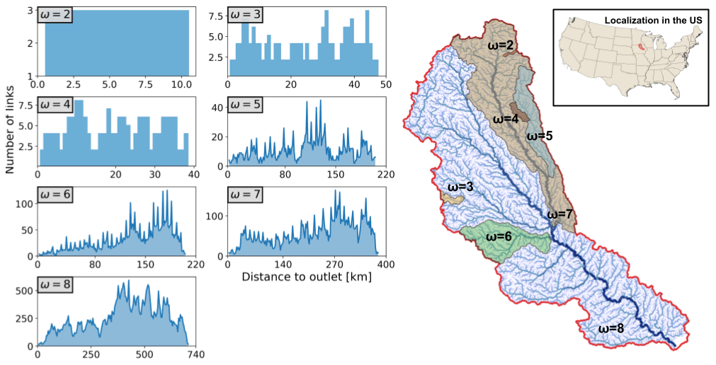
Figure 1 Cedar River watershed network structure (right) with the width function at the outlet (ω=8) and at nested subwatersheds with orders ω=2 to 7.

2.2 Development of hillslope-scale runoff fluctuations

In general, any rainfall pattern which is integrable over an interval of length can be written in terms of a Fourier series expansion as

$$\begin{array}{}\text{(3)}& p\left(t\right)={\displaystyle \frac{a_{\mathrm{0}}}{\mathrm{2}}}+{\sum }_{n=\mathrm{1}}^N{a}_n\cos \left({\displaystyle \frac{\mathrm{2}\mathit{\pi }nt}{T_r}}-{\mathit{\phi }}_n\right),\end{array}$$

where phase shifts allow us to represent sines (typically present in the Fourier series expansion) in terms of cosines of the same period. In this format, the coefficients can be chosen to sufficiently represent any function, including those that are not smooth.

We applied inverted and shifted cosines representing one, two, three, and four cosine waves distributed over the course of 1 or 3 d. The cosines were shifted to affirm that they were nonnegative and inverted – beginning and ending with zero precipitation intensity – to impose smoothness on the rainfall signal. We included both right-skewed and left-skewed sawtooth (linear) patterns and signals depicting uniform precipitation over 1, 2, 3, and 6 d.

Input to the model was applied as flux into a hillslope surface represented by a linear reservoir that feeds into the adjacent river link. Each input was designed to deliver 48 mm of water to the hillslope, and each signal began at time zero. Flow in the river network was primed by simulating a 1 d rainfall event and allowing the system to drain for 10 d before applying the rainfall signal so that each link of the river network had an initial flow that was commensurate with the watershed it drained.

2.3 Developing a reference hydrograph for each location in the river network

Comparing hydrographs across scales can be difficult due to the variability involved. To address this difficulty, we created dimensionless hydrographs for all locations in the river network with the following equations:

$$\begin{array}{}\text{(4)}& q^{\ast }={\displaystyle \frac{q}{q_{\mathrm{ref}}}}\text{and}{t}^{\ast }={\displaystyle \frac{t}{t_{\mathrm{ref}}}},\end{array}$$

where q_ref is a reference maximum streamflow, and t_ref is a reference hydrograph time to peak. For reference, we chose the instantaneous unit hydrograph that resulted from applying precipitation via a Dirac delta function, such that the volume of water was directly applied as an initial condition onto the hillslope surface, acting as an instantaneous event. From that hydrograph, we identified the peak flow and the time to peak flow for every link in the river network. We defined an event's end as the moment when the flow was smaller than 1 % of the peak flow.

2.4 Analysis of convergence of streamflow signals at larger scales

To analyze the convergence of the hydrographs for streams of order ω, we compared moments about the time axis (t^∗) and about the streamflow axis (q^∗). We computed the first moment in t^∗ and in q^∗ as

$$\begin{array}{}\text{(5)}& {\displaystyle }{M}_{\mathrm{1}}^{t^{\ast }}\left(\mathit{\omega }\right)={\displaystyle \frac{{\int }_{\mathrm{0}}^{T^{\ast }}{t}^{\ast }\cdot q^{\ast }\left(t^{\ast }\right)\mathrm{d}{t}^{\ast }}{{\int }_{\mathrm{0}}^{T^{\ast }}{q}^{\ast }\left(t^{\ast }\right)\mathrm{d}{t}^{\ast }}},\text{(6)}& {\displaystyle }{M}_{\mathrm{1}}^{q^{\ast }}\left(\mathit{\omega }\right)={\displaystyle \frac{{\int }_{\mathrm{0}}^{T^{\ast }}{q}^{\ast }\left(t^{\ast }\right)\mathrm{d}{t}^{\ast }}{{\int }_{\mathrm{0}}^{T^{\ast }}{t}^{\ast }\mathrm{d}{t}^{\ast }}},\end{array}$$

and we computed the second-centered moment with the following equations,

$$\begin{array}{}\text{(7)}& {\displaystyle }{M}_{\mathrm{2}}^{t^{\ast }}\left(\mathit{\omega }\right)={\displaystyle \frac{{\int }_{\mathrm{0}}^{T^{\ast }}(t^{\ast }-M_{\mathrm{1}}^{t^{\ast }}{)}^{\mathrm{2}}\cdot q^{\ast }\left(t^{\ast }\right)\mathrm{d}{t}^{\ast }}{{\int }_{\mathrm{0}}^{T^{\ast }}{q}^{\ast }\left(t^{\ast }\right)\mathrm{d}{t}^{\ast }}},\text{(8)}& {\displaystyle }{M}_{\mathrm{2}}^{q^{\ast }}\left(\mathit{\omega }\right)={\displaystyle \frac{{\int }_{\mathrm{0}}^{T^{\ast }}(q^{\ast }-M_{\mathrm{1}}^{q^{\ast }}{)}^{\mathrm{2}}\mathrm{d}{t}^{\ast }}{{\int }_{\mathrm{0}}^{T^{\ast }}{t}^{\ast }\mathrm{d}{t}^{\ast }}}.\end{array}$$

Using these definitions of moments, a ratio of the moments between two different hydrographs can be defined as

$$\begin{array}{}\text{(9)}& R_{i\left(A\mathrm{|}B\right)}^Z\left({\mathit{\omega }}_j\right)={\displaystyle \frac{max\left(M_i^z{\left({\mathit{\omega }}_j\right)}_A,M_i^z{\left({\mathit{\omega }}_j\right)}_B\right)}{min\left(M_i^z{\left({\mathit{\omega }}_j\right)}_A,M_i^z{\left({\mathit{\omega }}_j\right)}_B\right)}},\end{array}$$

where Z represents the variable of interest (in this case q^∗ and t^∗). If the moments of two different functions, A and B, approach each other, then Eq. (9) tends to 1 in the limit as

$$\begin{array}{}\text{(10)}& \begin{array}{c}\lim \\ \mathit{\omega }\to \mathrm{\infty }\end{array}{R}_{i\left(A\mathrm{|}B\right)}^Z\left(\mathit{\omega }\right)=\mathrm{1}.\end{array}$$

The min and max functions in Eq. (9) guarantee that the limit will be reached from above in all cases. This property allowed us to define a sigmoid function to characterize the rate of convergence to the limit of ω as

$$\begin{array}{}\text{(11)}& {\widehat{R}}_{i\left(B\right)}^Z\left(\mathit{\omega }\right)=S_{\mathrm{f}}\cdot \left(\mathrm{1}-{\displaystyle \frac{\mathrm{1}}{\mathrm{1}+e^{\left({\mathit{\omega }}_i-\mathit{\omega }\cdot \mathit{\alpha }\right)}}}\right),\end{array}$$

where S_f is a scale factor, ω_i is the starting Horton order, and α is a parameter controlling the shape of the curve. Larger values of α indicate rapid convergence of the curve to 1 as the Horton order of the basin increases; conversely, small values of α indicate slower convergence to 1.

3 Results

For each of the proposed input signals, we integrated the HLM routing equations using different assumptions about the distribution of velocity in space and time, including linear routing with constant velocity in space and time, nonlinear global self-similar routing, and locally self-similar nonlinear routing (Velásquez and Mantilla, 2020). For each setup, we obtained hydrographs at all the watershed links (43 000 in total). At the smaller scales ($\mathit{\omega }=\mathrm{2},\mathrm{3}$, or 4), each signal produced a distinct hydrograph. However, the hydrographs became indistinguishable with increasing Horton order.

3.1 Comparing hydrographs at multiple scales

In Fig. 2, we show the resulting hydrographs at multiple scales for input signals with a duration of 3 d. The top-left panel in Fig. 2 shows the different input signals used in this experiment. We chose locations in the river network corresponding to complete-order streams of orders 2 to 8 to illustrate differences in hydrograph shapes at different scales. The first set of graphs shows the hydrographs calculated under the assumption of constant flow velocity in the channels (i.e. λ₁=0 and λ₂=0) for locations with increasing Horton order. We repeated the calculation using more complex nonlinear routing assumptions. In the global self-similar case, we assumed v₀, λ₁, and λ₂ to be the same in the entire network (yellow shaded panels in Fig. 2), while in the local self-similar case the same parameters are variable throughout the catchment (green shaded panels in Fig. 2).

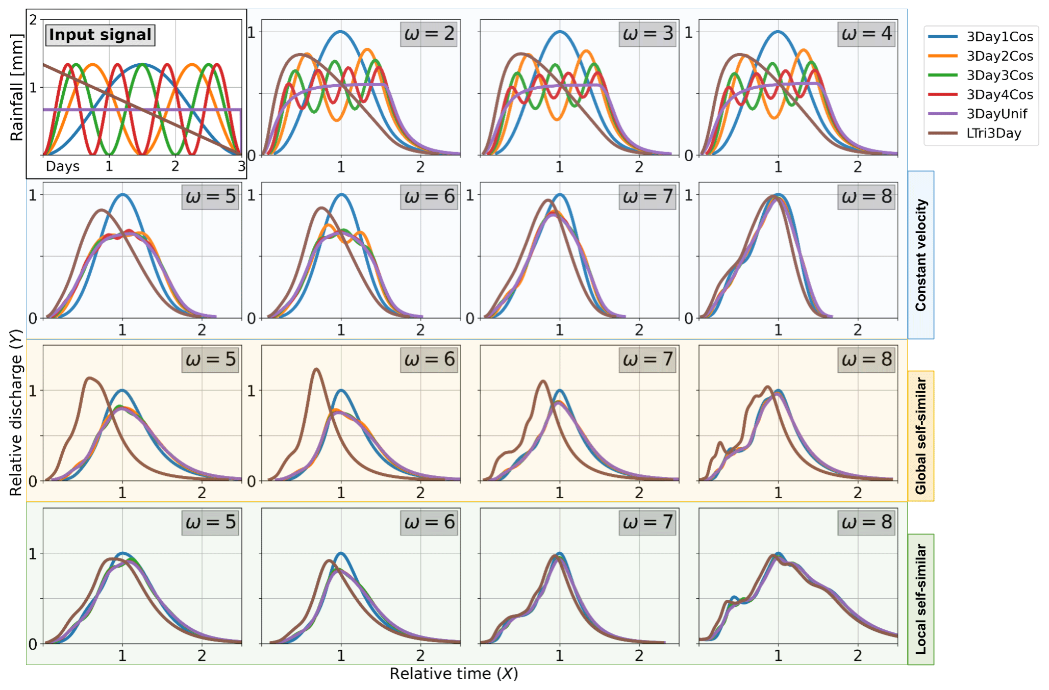
Figure 2 The 3 d duration input signals and resulting hydrographs at subwatersheds of orders between 2 and 8. The magnitude and time duration of the hydrographs is standardized relative to the 3Day1Cos (blue) hydrograph.

3.2 Convergence

In Fig. 2, we illustrate how all the 3 d duration signals tend to converge. Moreover, we can define the convergence of two or more signals relative to any signal by comparing their moments. Figure 3 shows the average value of R_A|B for the first (circles) and the second (triangles) moments when we compare moment ratios between the LTri3Day signal with the 3DayUniform one. In both dimensions (time and magnitude, Figures 3a and b, respectively), the value of R_A|B tends towards 1 with the increase of the Horton order. In the Supplement, we illustrate how the convergence of hydrographs occurs for all links in the network (Supplement Fig. S1). The convergence of hydrographs also holds for the more complex cases of nonlinear routing under the assumption of global and local self-similarity.

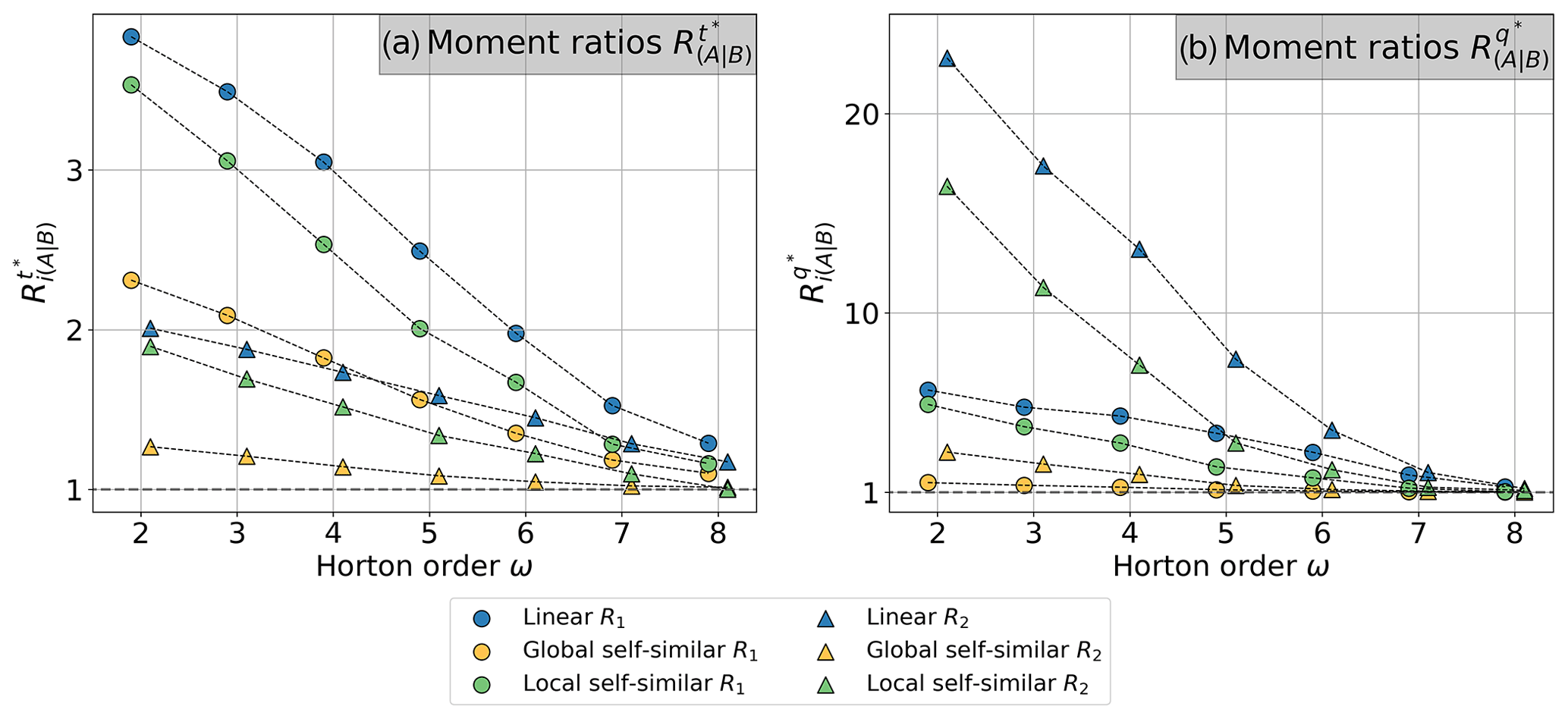
Figure 3 Changes of the first (circles) and second (triangles) moment ratios of the LTri3Day signal with respect to the 3DayUniform signal for different routing schemes. In panel (a), moment ratios are about the relative time $R_{i\left(B\right)}^{t^{\ast }}$, and in panel (b) moment ratios are about the relative streamflow $R_{i\left(B\right)}^{q^{\ast }}$.

3.3 General convergence to the instantaneous hydrograph (Dirac simulation)

To obtain a more general idea of the convergence, we computed R_A|B for all the input signals using the Dirac function as a reference. R_A|B at each Horton order ω was the median value obtained for all the links of order ω. The dots in Fig. 4 correspond to the computed median value of R_A|B. According to our results, each signal has a different R_A|B for ω=2 and, in all the cases, tends to converge toward 1 with increasing values of ω. Moreover, the convergence rate increases as a function of the initial differences. Signals with higher R_A|B values at ω=2 tend to converge at a faster rate than others.

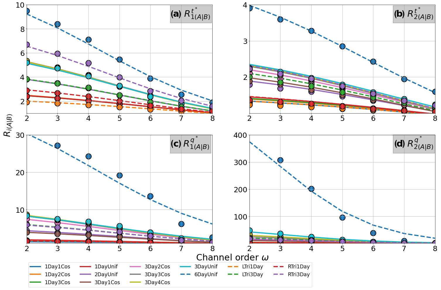
Figure 4 Convergence for all the signals relative to the Dirac simulation assuming constant velocity routing. The dots correspond to the median value of the moments ratio R, and the lines correspond to Eq. (11) results.

We describe the convergence rate of the median values in Fig. 4 using Eq. (11). In the equation, we fixed the scale factor S_f to 1.3, and we took ω_i=2 as the reference Horton order. Then, using the nonlinear least squares method, we adjusted the parameter α for a set of generated hydrographs. With this approach, we obtained a good representation of the signal's convergence starting at ω=2 (continuous lines in Fig. 4).

According to Fig. 4, the parameter α is an index of the convergence rate for any signal. Larger values of α correspond to faster convergence rates. Moreover, we found that α depends on the order of the moment, the dimension being considered (t^∗ or q^∗), and the streamflow routing approach. In Fig. 5, we present α vs. R_A|B(ω=2) for each moment order, dimension, and assumptions on the variability of velocities in space and time. In all cases, α was proportional to R_A|B(ω=2). This means that the greater the difference in the hydrographs at smaller scales, the faster the convergence rate to the Dirac shape at larger scales. The Supplement presents convergence for the nonlinear global and local self-similarity cases (Figs. S2 and S3).

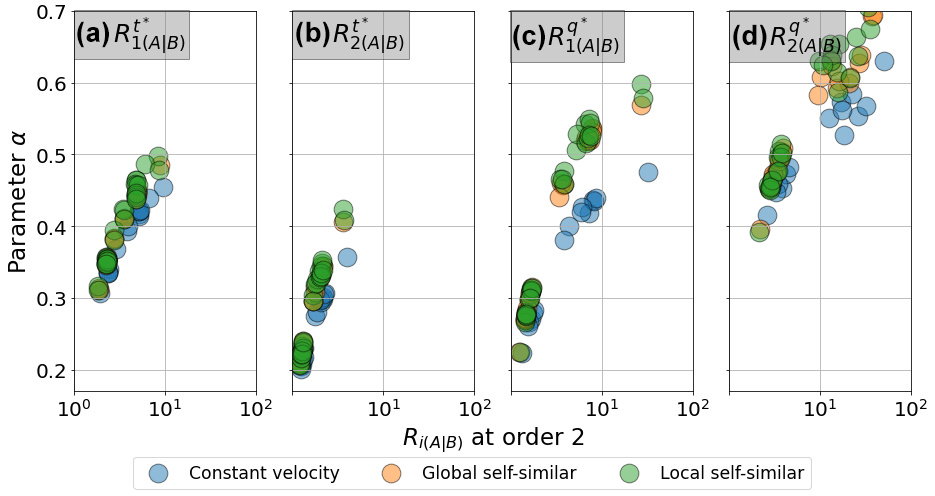
Figure 5 Values of the estimated parameter α as a function of moment ratios for hydrographs at order 2 streams for different scenarios of routing.

We found that the lower α values in the ratio of the second moment in time (Fig. 5b) correspond to lower values of R_A|B (Fig. 4b). Additionally, higher α values occur for the ratios of the second moment in q (Fig. 5d), which coincide with large R_A|B values (Fig. 4b). Also, we found that the convergence rates of the linear, nonlinear, and self-similar HLM setups are more alike in t^∗ than in q^∗.

4 Discussion and conclusions

Hydrologists strive to “be right for the right reasons” when modeling the hydrologic cycle; however, the datasets available to validate hydrological models are sparse and often comprise only streamflow observations at the outlets of large catchments. Typically, hydrologic modelers calibrate and validate their models using available streamflow observations. Our study sheds some new light on the limits of this strategy and provides an explanation for the difficulty in establishing a causal link between small-scale runoff generation processes and hydrograph shapes at the outlets of large river basins.

The moment ratios expressed in Eq. (9) show how hydrographs generated by different hillslope-scale runoff signals differ from each other across Horton order scales. Our study demonstrates that differences in the hydrographs at the hillslope scale are smoothed out for larger scales. The processes controlling the convergence rate are the spatial aggregation imposed by the self-similar river network draining the landscape and the attenuation that is controlled by the flow routing equations. Simulations not shown in this paper indicate that our results hold true for any self-similar network structure. However, a systematic analysis of how different network configurations determine the rate of convergence and if self-similarity is a necessary condition remains to be done. Two interesting findings of our study are that (i) the rate of convergence of hydrographs to a common shape at larger scales is proportional to how different the input signals are at the hillslope scale, and (ii) that the convergence is independent of the assumptions on the spatial and temporal variability of in-channel velocities imposed in the routing scheme.

Typically, validation of small-scale land-surface representations relies on the ability to reproduce streamflow hydrographs at the outlet of large catchments where historical records are available. An intermediate step in developing a site-specific hydrological model is calibrating its parameters that control the rainfall–runoff transformation (e.g., infiltration rates, hydraulic conductivity, interception rates) and runoff routing through the river network (e.g., channel and floodplain friction coefficients). Our results suggest that two very different descriptions of small-scale processes (e.g., variable saturated area vs. variable infiltration rates) can lead to equivalent hydrographs at larger scales. The fact that two competing hypotheses lead to the same result hampers the possibility of determining how changes in the small-scale process will affect streamflow hydrographs in larger catchments. Our analysis shows that the river network connectivity leads to an averaging of the runoff produced in different locations and at different times, indicating that if the right volume of runoff is applied at a given Horton-scale the hydrographs for the network of five orders or above would be indistinguishable.

The generic routing schemes tested in this study give us confidence that our results can be generalized to any hydrological distributed model of any basin that explicitly includes a river network with Horton–Strahler order 5 or larger. This extends the problem of model “equifinality” (Beven, 2006) to a larger problem of “equivalent models” where distinct descriptions of hillslope-scale descriptions lead to the same resulting outlet hydrograph.