Empirical stream thermal sensitivity cluster on the landscape according to geology and climate

Climate change is modifying river temperature regimes across the world. To apply management interventions in an effective and efficient fashion, it is critical to both understand the underlying processes causing stream warming and identify the streams most and least sensitive to environmental change. Empirical stream thermal sensitivity, defined as the change in water temperature with a single degree change in air temperature, is a useful tool to characterize historical stream temperature conditions and to predict how streams might respond to future climate warming. We measured air and stream temperature across the Snoqualmie and Wenatchee basins, Washington, during the hydrologic years 2015–2021. We used ordinary least squares regression to calculate seasonal summary metrics of thermal sensitivity and time-varying coefficient models to derive continuous estimates of thermal sensitivity for each site. We then applied classification approaches to determine unique thermal sensitivity regimes and, further, to establish a link between environmental covariates and thermal sensitivity regimes. We found a diversity of thermal sensitivity responses across our basins that differed in both timing and magnitude of sensitivity. We also found that covariates describing underlying geology and snowmelt were the most important in differentiating clusters. Our findings and our approach can be used to inform strategies for river basin restoration and conservation in the context of climate change, such as identifying climate-insensitive areas of the basin that should be preserved and protected.

1 Introduction

Globally, river temperature regimes are shifting in response to a changing climate. As water temperature is a critical component of aquatic ecosystems, these changes will alter an essential element of the habitat of many lotic organisms (Daufresne and Boët, 2007). To apply management interventions in an effective and efficient fashion, it is critical to both understand the underlying processes causing stream warming (Arismendi et al., 2014; Steel et al., 2017) and identify the streams most and least sensitive to environmental change (Parkinson et al., 2016; Pyne and Poff, 2017; Jackson et al., 2018). Measures of empirical stream thermal sensitivity, defined as the change in water temperature with a single degree change in air temperature or the slope of the statistical relationship between air temperature and water temperature, address both concerns.

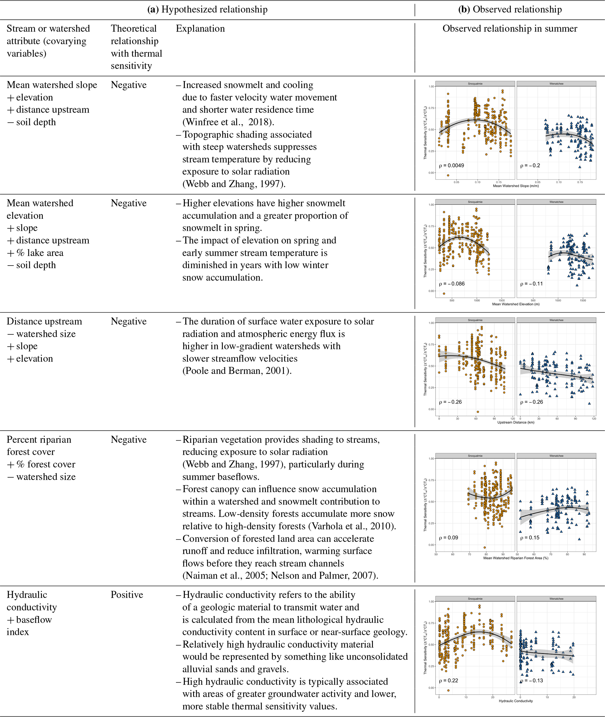
Thermal sensitivities reflect the combined influence of both spatially and temporally varying meteorological and hydrological factors, and a large body of literature examines hypothesized climate, landscape, and hydrogeologic drivers of thermal sensitivity (Table 1a). Variation in solar radiation is often the most important driver of both air and river temperatures, and as a result, air and river temperatures are typically correlated (Johnson, 2003; Leach et al., 2023). Landscape features such as riparian canopy cover and topographic shading associated with steep watersheds can reduce exposure to solar radiation, suppressing stream temperatures (Webb and Zhang, 1997). Stream temperature is also influenced by discharge through changes to thermal inertia and residence time (Meier et al., 2003) and runoff composition where snowmelt, surface runoff, and groundwater inflow entering the stream have different temperature signatures than the stream itself (Webb and Zhang, 1997; Mohseni and Stefan, 1999; Cadbury et al., 2008). Inputs from water sources such as snowmelt and groundwater upwelling decouple air and water temperatures and result in a decreased thermal sensitivity of water temperature to air temperature (Tague et al., 2007; Mayer, 2012; Johnson et al., 2014). As a result, the relationship between air and water temperatures can also be a useful diagnostic tool for identifying putative hydrological processes for which empirical measures are often unavailable. Thermal sensitivity has been used in the past to estimate areas of shallow and deep groundwater influence (Snyder et al., 2015; Briggs et al., 2018) and to understand the role of snowmelt in modulating river temperature (Lisi et al., 2015; Winfree et al., 2018). Despite conceptual agreement about hypothesized drivers of thermal sensitivity, substantial uncertainty persists regarding the relative importance of these covariates in controlling and predicting thermal sensitivity.

Table 1 Hypothesized relationships between landscape covariates and thermal sensitivity based on the previous literature (a) and the observed relationship between landscape variables and thermal sensitivities within our study basins in summer (b). Loess curves are shown to aid in visualization and correlation coefficients quantify the strength of the linear relationship. See Fig. S6 in the Supplement for a detailed description of how river attributes covary with one another.

Empirical stream thermal sensitivity has been widely used to characterize historical stream temperature conditions and to predict how streams might respond to future climate warming (Mohseni et al., 2003; Mantua et al., 2010). Generally, larger thermal sensitivities indicate that water temperatures are more likely to track changes in air temperature (Isaak et al., 2016, 2018a; Mauger et al., 2017). However, there are concerns about using present-day thermal sensitivities to predict future stream temperatures, as it can be difficult to derive insights into river responses to perturbations from statistical models that rely on historical relationships that may not extrapolate well to future conditions. For example, past studies have found that using empirical relationships for extrapolating to future climate scenarios without accounting for underlying processes such as snowmelt, groundwater, and annual hysteresis may provide inaccurate predictions of future stream temperatures (Leach and Moore, 2019; Steel et al., 2019). Under changing climatic conditions, the interrelations between air temperature and other processes controlling stream temperature may not remain stable (Arismendi et al., 2014). Additionally, stream networks can exhibit patchy thermal conditions due to spatially heterogeneous landscape attributes such as riparian shading, valley form and aspect, and geology (Bogan et al., 2003; Benyahya et al., 2010). Large-scale models that do not incorporate fine-scale variation into thermal sensitivity may not accurately predict thermal habitat at ecologically relevant scales. Despite these shortcomings, thermal sensitivity remains a commonly used and straightforward tool that allows for comparison between locations within rivers and has the potential to guide management.

There is a need to better understand how thermal sensitivities evolve throughout the year and along river networks and to develop a clearer understanding of the relationships between derived model coefficients and important watershed processes. Furthermore, thermal sensitivity itself can vary across time and space, rendering stationary values insufficient to describe variability in this parameter. A clearer vision of how thermal sensitivities vary would allow natural resource managers to understand what a single snapshot in time or space represents and could provide insight into how river thermal sensitivity may evolve under nonstationary air temperature and precipitation regimes. Groups of streams (clusters) that share similar patterns of thermal sensitivity will likely also share similar risk profiles. Identification of stream clusters could help managers tailor investment in streams according to watershed-specific influences (Mayer, 2012). This study aims to answer the following questions across two Pacific Northwest river basins. (1) What is the spatial and temporal distribution of commonly used thermal sensitivity metrics across each basin? (2) What are the representative thermal sensitivity regimes, how do they cluster on the landscape, and how do these clusters differ from clusters based on air and water temperature individually? (3) What are the landscape or climate factors that best predict thermal sensitivity cluster membership? Finally, we consider the statistical functionality of these methods in river networks.

2 Methods

2.1 Study area

The Snoqualmie River begins as three distinct forks in the Mt. Baker Snoqualmie National Forest and drains a 1813 km² watershed on the western side of the Cascade Range, Washington (Fig. 1). The three forks originate in forested public land before converging and flowing through a mix of agricultural, residential, and commercial land use. In one major tributary, the Tolt River, a dam and a large reservoir provide drinking water for the city of Seattle (Fig. S4). The Wenatchee River drains 3440 km² of the eastern Cascades before flowing into the Columbia River (Fig. S5). Although land use is similar to the Snoqualmie basin, wherein the headwaters originate in forested public lands before flowing through a mix of agricultural, residential, and commercial land use, forest density is generally lower in the eastern Cascades.

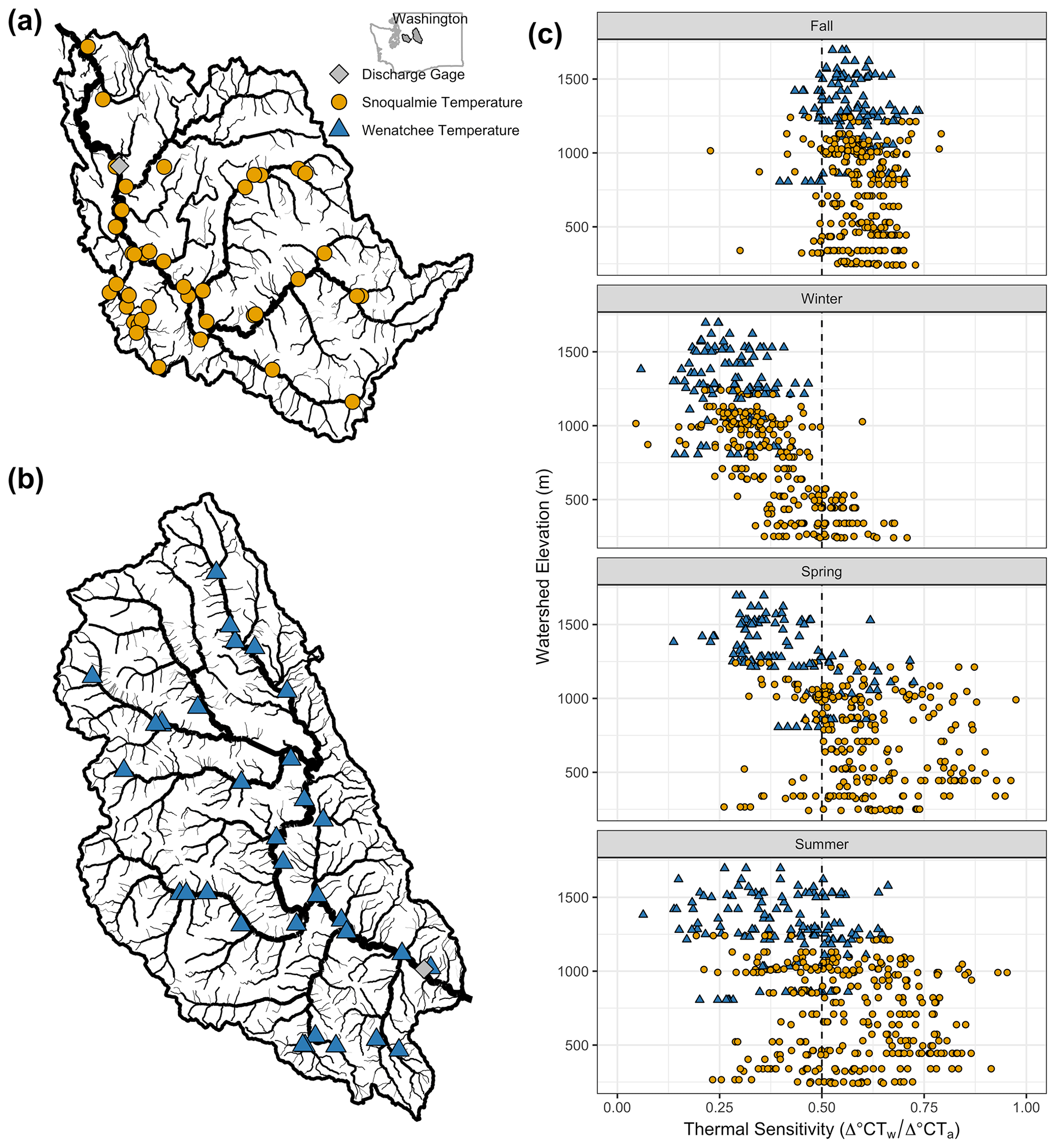
Figure 1 A map of the Snoqualmie (a) and Wenatchee (b) basins' water and air temperature monitoring sites as well as the most downstream USGS gage for each basin. Thermal sensitivity, defined as the change in water temperature with a single degree change in air temperature, versus mean watershed elevation (MWE) for each site–year combination (c). The dashed line in panel (c) is included as a reference.

Both the Snoqualmie and Wenatchee basins have a Mediterranean climate with dry summers and wet, mild winters influenced by proximity to the Pacific Ocean. The climate on the eastern side of the Cascades is drier than that of the western side; the average annual precipitation is 1874 mm (939 mm) and the average annual temperature is 5.7 °C (5.3 °C) for the western (eastern) Cascades. However, the prevailing westerly winds, which cross the Cascades, create temperature and precipitation gradients that vary widely across the Wenatchee basin. In both basins, precipitation occurs predominately from October to March. The coldest month is typically January, whereas the warmest is July. Rivers have a mixed rain–snow hydrology with substantial winter rain and spring snowmelt, although the Wenatchee basin receives more winter precipitation as snow. Peak flow generally occurs during winter in the Snoqualmie River and spring in the Wenatchee River (Fig. 2). The geology differs across the basins. The geology of the Snoqualmie basin is characterized by a deep glacial aquifer in the lowland portion of the watershed, whereas in the alpine area much of the ground surface is directly underlain by bedrock that lacks significant fracture systems (Turney et al., 1995; Bethel, 2004). In contrast, the Wenatchee basin's geology consists of both an aquifer within the sedimentary bedrock of the central and lowland areas and an overlying unconsolidated alluvial and outwash aquifer located primarily in river valley bottoms (Montgomery Water Group, 2003). The Snoqualmie and Wenatchee basins both have reaches where water temperature exceeds regulatory thresholds established for salmonids that are protected by the US Endangered Species Act (ESA). Both basins support ESA-listed Chinook salmon (Oncorhynchus tshawytscha) and steelhead trout (Oncorhynchus mykiss), and the Wenatchee basin additionally supports populations of bull trout (Salvelinus confluentus) and sockeye salmon (Oncorhynchus nerka).

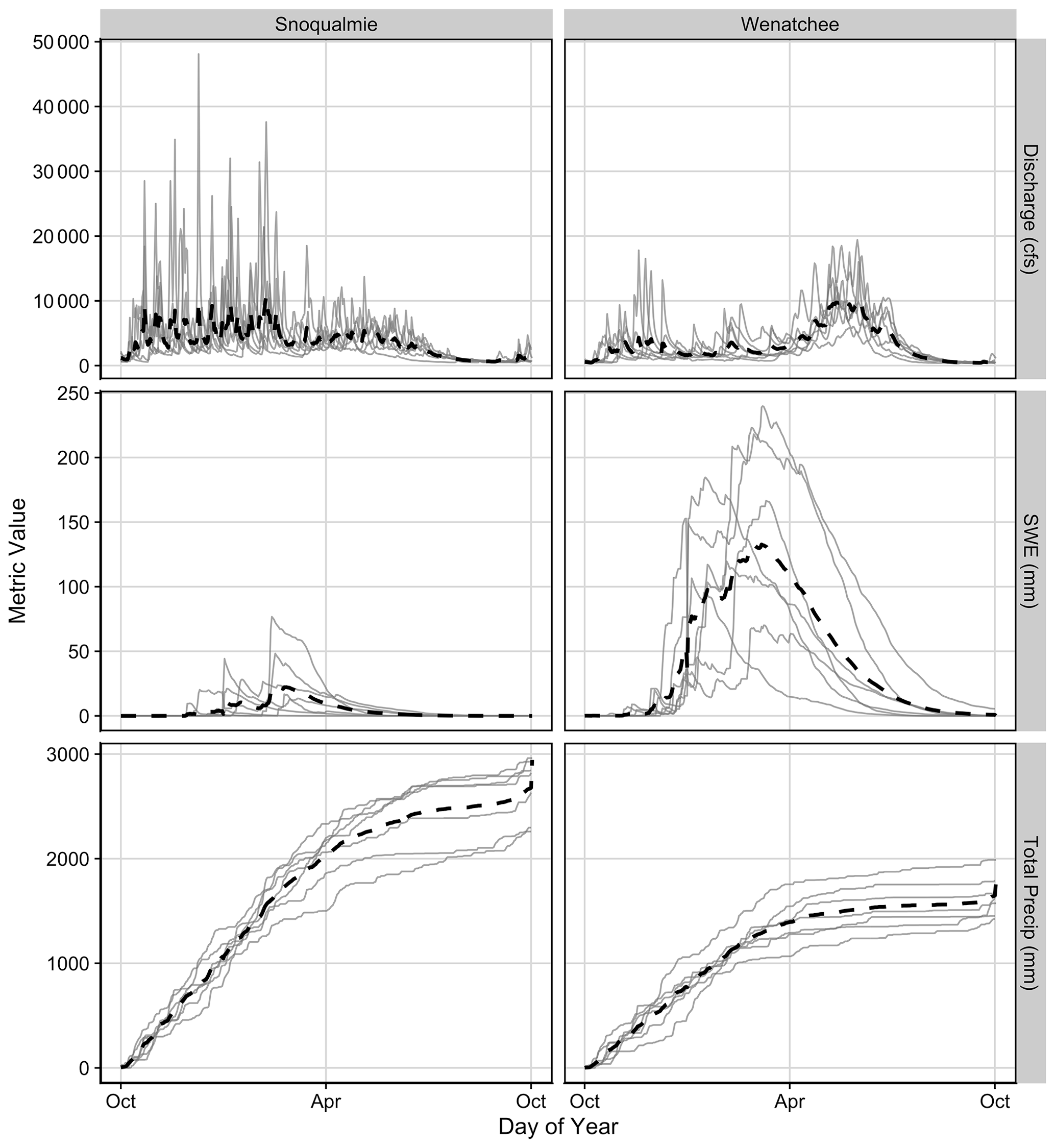
Figure 2 Average annual discharge, snow water equivalent (SWE), and total precipitation for the outlets of the Snoqualmie and Wenatchee basins across the sampling time frame (black dashed lines) and interannual variability across the 7 water years included in this analysis (2015–2021, gray lines). Discharge gage locations can be found in Fig. 1a and b, and SWE and precipitation data are from DAYMET Daily Surface Weather data for the upstream watershed of each discharge gage (Thornton et al., 2020).

Water temperature loggers (N_Snoqualmie= 42, N_Wenatchee= 31) were installed throughout the mainstems, on major tributaries, and on a selection of minor tributaries for both the Snoqualmie and Wenatchee rivers (Fig. 1). Practical limitations forced sites to be publicly accessible, on private property with landowner permission, and within 1 km of a road. For this study, water temperature was recorded using HOBO TidbiT v2 (UTBI-001) loggers every hour from 1 October 2014 through 30 September 2021 in both basins. We hereafter use North American hydrologic years (1 October–30 September) instead of calendar years with the year of summer data as the year of reference. Air temperature data were recorded using HOBO Pendant (UA-002-64) loggers every hour at all water temperature monitoring sites. Air temperature was logged for a subset of 11 (6) sites in the Snoqualmie (Wenatchee) basin beginning on 1 October 2014 and for all sites beginning on 1 October 2016 (1 October 2018). Air loggers were placed on trees along the stream bank as close to the stream temperature loggers as possible. The air temperature loggers were secured at approximately breast height on the northern side of the trees. Solar shields were fashioned to house both water and air temperature loggers. All air and water temperature data for the Wenatchee basin logged prior to 1 October 2018 were collected by the Washington Department of Ecology (Washington Department of Ecology, 2023).

2.2 Exploratory analysis of air–water correlation summary metrics

We calculated two summary metrics to characterize the relationship between air temperature and water temperature. For each site, summary metrics were derived from linear regressions between mean daily values of air and water temperature. The slope of this relationship, the thermal sensitivity, indicates the average difference in water temperature when comparing time periods with a 1° difference in air temperature. For example, a thermal sensitivity of 0.5 would indicate that, based on historical data, when air temperature at a site differs by 1 °C, water temperature differs on average by 0.5 °C (Leach and Moore, 2019). The strength of this relationship (R²) is an indicator of how well water temperature can be approximated by air temperature and is calculated as the Pearson correlation value between air and water temperature. Summary metrics were calculated separately for each season. Seasons were defined as fall (October, November, December), winter (January, February, March), spring (April, May, June), and summer (July, August, September).

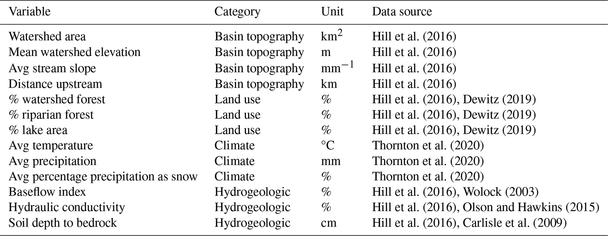
Watersheds for each site were delineated and covariates describing the watersheds were obtained from commonly available geostatistical products (Table 2). Covariates were divided into four broad categories: basin topography (watershed area, mean watershed elevation, average stream slope, and distance upstream), land use (percent watershed forest, riparian forest, and lake area), climate (average temperature, precipitation, and percent precipitation falling as snow), and hydrogeology (baseflow index, hydraulic conductivity, and soil depth to bedrock). Temperature, precipitation, and percent precipitation as snow were obtained from DAYMET Daily Surface Weather data (Thornton et al., 2020), and all the other landscape covariates were obtained from the Stream-Catchment (StreamCat) database (Hill et al., 2016).

Table 2 Physical environmental data and basin characteristics used to predict air–water clusters.

A large body of literature examines landscape-level drivers of air and water temperature correlations within rivers. Therefore, we first summarized hypothesized drivers of thermal sensitivity based on the previous literature and their covarying landscape variables within our basins (Table 1a). We then conducted an exploratory analysis of the relationship between landscape covariates and thermal sensitivity to better understand patterns in our data and set up future hypothesis testing. Due to the correlated nature of our dataset, no formal statistical tests were conducted. We plotted summer thermal sensitivity against hypothesized drivers, including mean watershed elevation (MWE), watershed slope, distance upstream, percent riparian forest cover, and substrate hydraulic conductivity. Loess curves were plotted to aid in data visualization, and correlation coefficients between thermal sensitivity and each landscape covariate were used to quantify the strength of the linear relationship.

We also explored the relationship between spring thermal sensitivity and snowmelt, defined as the change in snow water equivalent (SWE) for a given season and denoted as ΔSWE, and between summer thermal sensitivity and mean air temperature and total precipitation. Climatic variables were obtained from gridded DAYMET data products (Thornton et al., 2020) and calculated for the upstream catchment of each monitoring station.

2.3 Spatially weighted clustering of thermal sensitivity, water temperature, and air temperature

To identify representative regimes of air–water temperature correlations, we employed a varying-coefficient linear model to obtain continuous, daily estimates of thermal sensitivity. We then defined a spatially weighted dissimilarity matrix for use in clustering, which quantifies the spatial correlation in thermal sensitivity time series while accounting for the directed river network structure. We used this spatially weighted dissimilarity matrix with agglomerative hierarchical clustering to identify groups of sites exhibiting similar patterns in thermal sensitivity over time and compared these clusters to those generated using only water or air temperature. The details of each step are provided in the following sections.

2.3.1 Varying coefficient linear model for air–water relationships

To derive a continuous thermal sensitivity metric, we fit a time-varying coefficient model (TVCM) to air and water temperature data. The TVCM is an effective tool for exploring dynamic features of the sensitivity of water temperature with changes in air temperature and uses a parametric linear model but with time-varying coefficients (Li et al., 2014, 2016). For a given site, we described the varying coefficient model for the air–water temperature relationship as

$$\begin{array}{}\text{(1)}& y_t={\mathit{\beta }}_{\mathrm{0},t}+x_t{\mathit{\beta }}_{\mathrm{1},t}+{\mathit{ϵ}}_t,t=\mathrm{1},\mathrm{\dots },T,\end{array}$$

where β_0,t and β_1,t are varying intercept and slope coefficients. To estimate the time-varying coefficients, we adopted an ordinary least squares kernel regression with the Nadaraya–Watson estimator, where we fit a set of weighted local regressions with an optimally chosen window size defined by the bandwidth, b, and the weights given by the kernel function (Hoover, 1998; Casas and Fernandez-Casal, 2019). The kernel and its bandwidth control the level of smoothing by adjusting the weight that the neighboring time points have on estimates at t. The bandwidth was set to 0.2 a priori to ensure consistency across time series. We used the Gaussian kernel that is of the form $k\left(x\right)=\frac{\mathrm{1}}{\mathrm{2}}\mathit{\pi }{e}^{-\frac{x^{\mathrm{2}}}{\mathrm{2}}}$. The varying intercept term represents the mean water temperature at time t, and the varying slope term represents the local sensitivity of water temperature to changes in air temperature at time t. We used the R package tvReg (Casas and Fernandez-Casal, 2021) to implement the model.

We filtered resultant time series for site years with > 218 d (60 % of the year) and gaps of ≤ 7 d, yielding 250 site years from 73 sites across both the Snoqualmie and Wenatchee basins. To capture the typical range and timing of thermal sensitivity at each site, we created a single representative time series of thermal sensitivity at each site by calculating the mean daily thermal sensitivity for each day of the year across all the years of filtered data. We use this average annual time series for subsequent clustering analyses. To ensure that using an average annual time series of thermal sensitivity was an appropriate choice given the structure of our data, we conducted a supplementary analysis to assess cluster sensitivity to interannual variability (Sect. S1 “Interannual variability in thermal sensitivity” in the Supplement). Measured air and water temperature and modeled thermal sensitivities for each site can be visualized at the following link: https://lmcgill.shinyapps.io/TimeVarying_AWC/ (last access: 4 March 2024; McGill, 2024).

2.3.2 Estimating a spatially weighted dissimilarity matrix

To quantify spatial correlation while accounting for the directed river network structure, we developed a dissimilarity measure for time series of thermal sensitivity, water temperature, and air temperature that incorporated spatial correlation between sites (Haggarty et al., 2015). The general form of the proposed dissimilarity measure between sites x and y can be written as

$$\begin{array}{}\text{(2)}& d_{xy}^{\mathrm{c}}=d_{xy}\widehat{\text{cov}}\left(h_{\mathrm{s}}\right),\end{array}$$

where $d_{xy}^{\mathrm{c}}$ is the spatially weighted dissimilarity matrix, d_xy is the Canberra distance (Lance and Williams, 1967), and $\widehat{\text{cov}}\left(h_{\mathrm{s}}\right)$ is a valid stream-distance-based covariance matrix.

To estimate $\widehat{\text{cov}}\left(h_{\mathrm{s}}\right)$, we used the tail-down model that was introduced by Ver Hoef and Peterson (2010). Due to the complex structure of the tail-down model, it is necessary to model spatial correlation on a river network with a covariogram. We first estimated the covariance between time series at each site using a classic formula from Cressie (1993), which states that the estimated covariance between sites x and y is given by

$$\begin{array}{}\text{(3)}& \widehat{\text{cov}}\left(x,y\right)=\sum _{t=\mathrm{1}}^T{\displaystyle \frac{\left\{x_t-\stackrel{\mathrm{‾}}{x}\right\}\left\{y_t-\stackrel{\mathrm{‾}}{y}\right\}}{T}},\end{array}$$

where x_t and y_t are the values of the variable (thermal sensitivity, water temperature, or air temperature) at sites x and y at time t and T is the total number of discrete times. This results in a single value which summarizes the covariance between the time series at the two sites over the period of interest. We then plotted these point summaries of the covariance between pairs of curves against lags (measured as stream distance) to obtain an empirical stream-distance-based covariogram. We fit an exponential covariance function to this empirical covariogram and evaluated the model at relevant distances to obtain an estimated stream-distance-based covariance matrix $\widehat{\text{cov}}\left(h_{\mathrm{s}}\right)$. We used this new covariance matrix to weight the Canberra distance matrix as shown in Eq. (2). The final spatially weighted dissimilarity matrix, $d_{xy}^{\mathrm{c}}$, was then used in clustering analyses.

2.3.3 Agglomerative hierarchical clustering

We used agglomerative hierarchical clustering (AHC) to identify groups of sites where the patterns in thermal sensitivity, water temperature, and air temperature were similar over time using the hclust function in R (R Core Team, 2022). AHC is a common clustering method (Olden et al., 2012; Maheu et al., 2016; Savoy et al., 2019; Isaak et al., 2020) where each time series starts in its own cluster and the hierarchy is built by repeatedly merging pairs of similar clusters separated by the shortest distance (i.e., measured as the similarity between individual time series) until all points are contained in a single cluster. To decide which clusters are merged in every iteration, AHC uses a dissimilarly metric ($d_{xy}^{\mathrm{c}}$, derived in Eq. 2) and a linkage criterion. We used Ward's minimum variance linkage method for clustering, where the distance between two clusters is computed as the increase in the sum of squared differences after combining two clusters into a single cluster. The shortest of these links (minimum increase in the sum of squared differences) that remains at any step causes the fusion of the two clusters whose elements are involved.

A difficulty associated with cluster analysis is determining the most appropriate number of clusters given the data because no a priori optimal number of clusters exists. Clusters resulting from alternative choices can be evaluated through internal cluster validity indices (CVIs); there are a variety of CVIs, most of which combine within-cluster cohesion (intra-cluster variance) and between-cluster separation (inter-cluster variance) to compute a quality measure. There is no universally best CVI (Arbelaitz et al., 2013), and therefore we calculated a suite of five CVIs, including the Silhouette, Gap, Davies–Bouldin, Calinski–Harabasz, and generalized Dunn indices, using the NbClust R package (Charrad et al., 2014). A final number of clusters was determined by a majority-rules approach based on the optimal number of clusters suggested by each index (Table S2 in the Supplement).

To determine whether cluster assignments were stable or preserved in a perturbed dataset similar to the original one and therefore likely reflective of real differences, we conducted a bootstrapping approach where sites were sampled with replacements, and then AHC was performed on the resampled data using the fpc R package (Hennig, 2020). For each bootstrapped cluster, we assessed the similarity between each new cluster and the most similar original cluster with the Jaccard index. The Jaccard coefficient ranges from 0 to 1. Clusters with a coefficient larger than 0.75 were considered stable and clusters with a coefficient between 0.5 and 0.75 indicate that the cluster is measuring a pattern in the data, but exact site assignment may be doubtful and clusters with a mean Jaccard coefficient of less than 0.5 were considered unstable and may not reflect a true pattern in the data (Maheu et al., 2016; Savoy et al., 2019). We repeated the bootstrapping procedure 10 000 times; the mean Jaccard coefficient for each cluster is reported in Table 4.

2.3.4 Identification of environmental drivers in thermal sensitivity

We used classification and regression trees (CARTs; Breiman et al., 1984) to investigate the relative importance of basin topography, land use, climate, and hydrogeologic attributes (Table 2) for predicting each site's membership in a thermal sensitivity cluster. A CART is typically used to attempt to predict membership in clusters using environmental attributes, and it allows the modeling of nonlinear relationships among mixed variable types and facilitates the examination of intercorrelated variables in the final model (De'ath and Fabricius, 2000; Olden et al., 2008). We took an exploratory approach to this analysis due to our relatively small sample size (N_Snoqualmie= 42, N_Wenatchee= 31), which limited our ability to conduct statistical tests. Therefore, we calculated variable relative importance, defined as the sum of squared improvements at all splits determined by the predictor. These values are scaled to sum to 100 (rounded). To ensure no single site unduly impacted CART results (Krzywinski and Altman, 2017), we conducted a supplementary leave-one-out cross-validation analysis to ensure relative importance estimates were stable across different permutations of the data (Fig. S7). We used the R package rpart (Therneau and Atkinson, 2019) to implement the CART model.

3 Results

3.1 General patterns in temperature, precipitation, and thermal sensitivity

This analysis included data from 7 hydrologic years, each with differing temperature and precipitation patterns. Generally, the years spanned by our dataset were warmer than the historical average (1901–2000), with wetter-than-average winter and fall months and drier spring and summer months (Fig. S1). For the western (eastern) Cascades, all the years (2015–2021) have average annual temperatures higher than the long-term average of 8.6 °C (3 °C), although individual seasons were slightly cooler than average. The year 2015 stood out as a year with an exceptionally warm winter, low snowpack, and dry spring. Temperature and precipitation patterns in the western and eastern Cascades were generally similar; however, precipitation anomalies were typically smaller in the eastern Cascades due to the overall lower precipitation in this region (Figs. 2 and S1).

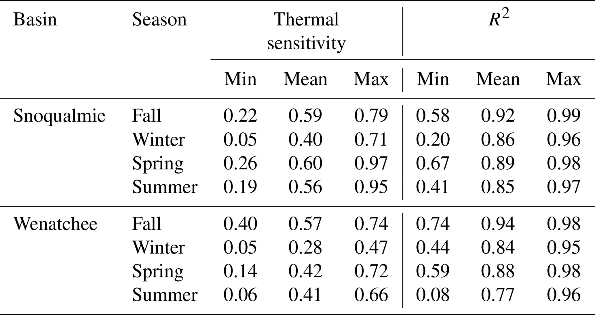
Summary metrics describing air–water temperature relationships exhibited substantial variation across time (season and year) and space. Across all the season–year combinations, thermal sensitivities ranged from 0.05 to 0.97 (mean = 0.54) in the Snoqualmie basin and from 0.06 to 0.74 (mean = 0.42) in the Wenatchee basin (Table 3). Seasonal distributions of thermal sensitivities also differed. For example, fall thermal sensitivities in both basins were relatively homogeneous, with 90 % of the values falling between 0.47 and 0.70, whereas spring and summer thermal sensitivities exhibited a broader range of values, with 90 % of the values falling between 0.30 and 0.84 in spring and between 0.25 and 0.78 in summer. Air temperature was generally a good predictor of water temperature, as evidenced by R² values that ranged from 0.20 to 0.99 (mean = 0.88) in the Snoqualmie basin and from 0.08 to 0.98 (mean = 0.85) in the Wenatchee basin (Table 3).

Table 3 Air–water correlation average summary metrics by basin and season. Averages are calculated as the mean value of summary metrics at all the sites across each basin and season.

Overall, weak and inconsistent patterns emerge in summer between thermal sensitivity and landscape and climate variables (Fig. 3; Table 1b). For climate variables, only ΔSWE appeared to have a relationship with thermal sensitivity (Fig. 3). The relationship between ΔSWE and thermal sensitivity was negative and nonlinear, displaying a wedge-shaped pattern wherein large snowmelt events did not reduce thermal sensitivities below 0.25 (Fig. 3). For landscape variables, correlation coefficients were overall small ($\left|\mathit{\rho }\right|<$ 0.3), indicating weak to non-existent linear relationships between landscape covariates and observed thermal sensitivity (Table 1b). A weakly negative relationship between thermal sensitivity and distance upstream was observed for both basins. Percent riparian forests and thermal sensitivity showed no relationship for either basin. The relationship between hydraulic conductivity and thermal sensitivity was weakly positive and parabolic in the Snoqualmie basin.

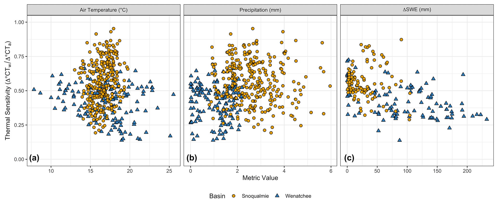
Figure 3 Summer thermal sensitivity values for all site–year combinations in the Snoqualmie and Wenatchee basins versus air temperature (a) and precipitation (b). Spring thermal sensitivity values for all site–year combinations versus the total snow water equivalent (SWE) (c) from gridded DAYMET data for each sampling point. Points are colored by basin. Basins that have no snowmelt in a given year are not shown in panel (c).

3.2 Patterns of clustering for water temperatures, air temperatures, and thermal sensitivities

Time-varying thermal sensitivities displayed periods of both high and low values within a season, which was not necessarily represented when looking only at seasonal summary metrics (Figs. 4 and 5). Thermal sensitivity varied alongside water and air temperature within the Snoqualmie and Wenatchee basins. Generally, thermal sensitivity rose sharply in late spring, was highest in late summer, declined slowly throughout the fall, and remained depressed through winter and early spring.

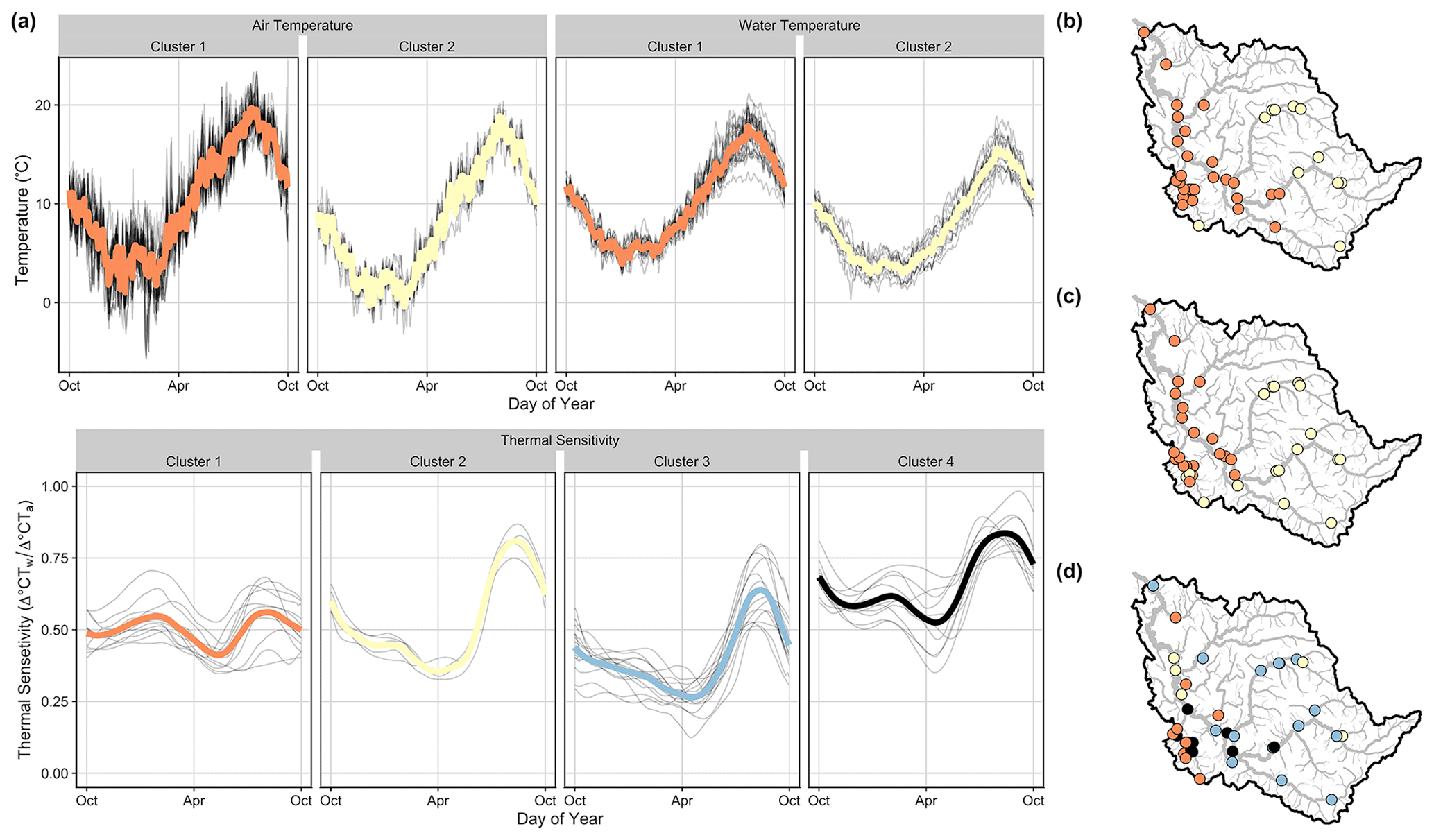
Figure 4 Average time series (a) and spatial clustering results (columns and colors indicate unique clusters) for average annual air temperature (b), water temperature (c), and thermal sensitivity (d) in the Snoqualmie basin. The colored lines indicate mean average annual values for each cluster, and gray lines denote average annual values for each site within a given cluster.

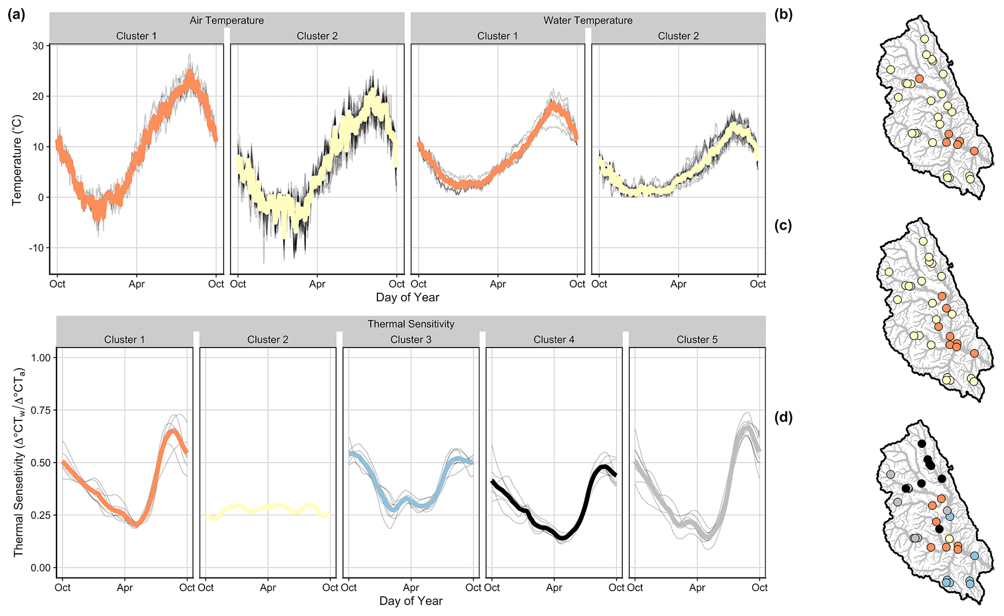
Figure 5 Average time series (a) and spatial clustering results (columns and colors indicate unique clusters) for average annual air temperature (b), water temperature (c), and thermal sensitivity (d) in the Wenatchee basin. The colored lines indicate mean average annual values for each cluster, and gray lines denote average annual values for each site within a given cluster.

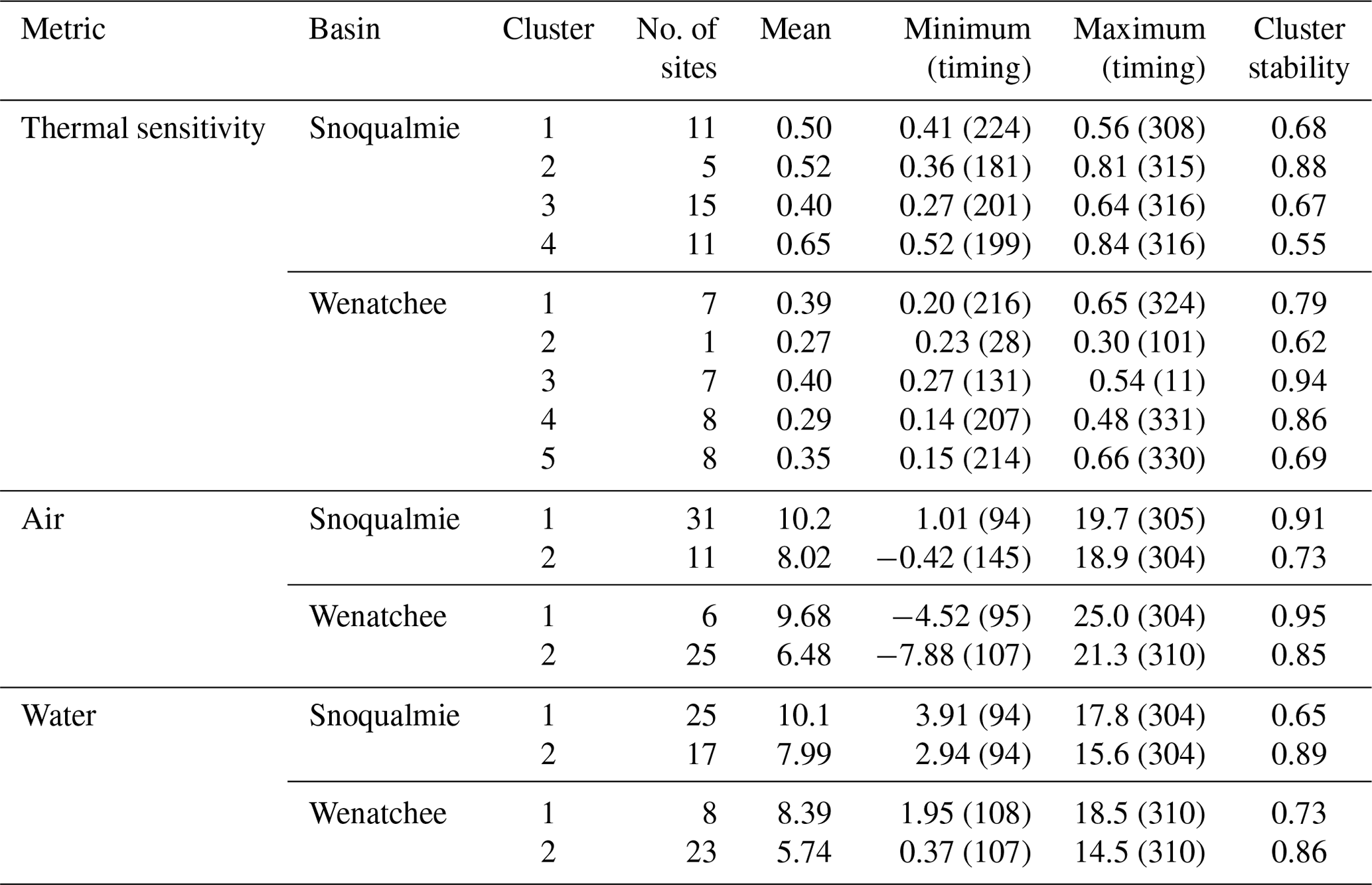
Spatially weighted AHC yielded four clusters for thermal sensitivity, with a CVI range of 2–4, two clusters each for air (CVI range of 2–5) and water (CVI range of 2–4) temperature in the Snoqualmie basin, five clusters for thermal sensitivity (CVI range 2–5), and two clusters each for air (CVI range of 2–3) and water (CVI range of 2–5) temperature in the Wenatchee basin (Figs. 4 and 5; Table S2). For both basins, clusters of air and water temperature correspond closely to elevational gradients (Figs. S4 and S5). Higher-elevation sites exhibited generally lower magnitudes but similar patterns in air and water temperatures (Table 4). For example, within both basins, seasonal water temperatures were synchronized, with the cluster minimum and maximum water temperatures occurring within a day of each other (Table 4). In the Snoqualmie basin, air temperature clusters were stable, with mean Jaccard indices of 0.91 for high-elevation sites (Cluster 2, n= 11 sites) and 0.73 for low-elevation sites (Cluster 1, n= 31 sites). Water temperature clusters were slightly less stable, with mean Jaccard indices of 0.65 for high-elevation sites (Cluster 2, n= 17 sites) and 0.89 for low-elevation sites (Cluster 1, n= 25 sites). Air and water temperature clusters in the Wenatchee basin were more stable than the Snoqualmie clusters. In the Wenatchee basin, air temperature clusters had mean Jaccard indices of 0.85 for high-elevation sites (Cluster 2, n= 25 sites) and 0.95 for low-elevation sites (Cluster 1, n= 6 sites), and water temperature clusters had mean Jaccard indices of 0.86 for high-elevation sites (Cluster 2, n= 23 sites) and 0.73 for low-elevation sites (Cluster 1, n= 8 sites).

Table 4 Averaged metrics for all sites within each cluster determined with the spatially weighted agglomerative hierarchical clustering. For timing metrics, days are reported as hydrologic day, where a value of 1 indicates 1 October and a value of 365 indicates 30 September.

Clustering patterns for thermal sensitivity were more complex and less stable than air and water temperature clusters, particularly for the Snoqualmie basin (Figs. 4 and 5; Table 4). In the Snoqualmie basin, Cluster 1 (n= 11 sites) consisted primarily of low-elevation tributaries that exhibited stable thermal sensitivities throughout the year, producing a cluster-average range of only 0.15 (Fig. 4; Table 4). Cluster 2 was small (n= 5 sites), and the distribution of sites within this cluster included three mainstem sites and two high-elevation tributaries. Despite the large geographic distances separating sites, this cluster was highly stable with a mean Jaccard index of 0.88. Cluster 2 was characterized by a mean thermal sensitivity of 0.52 and the highest annual variability, with a cluster-average range of 0.45. Cluster 3 was large (n= 15 sites) and contained sites located within the upper regions of the Snoqualmie River. Cluster 3 had the lowest mean thermal sensitivity (mean = 0.40). Lastly, Cluster 4 (n= 11 sites) exhibited the lowest stability of any cluster in the Snoqualmie basin, with a mean Jaccard index of 0.55. Sites in this cluster were mainly situated on the mainstem Snoqualmie and its major tributaries. This cluster was distinguished by the highest mean thermal sensitivity (mean = 0.65). In the Wenatchee basin, all five thermal sensitivity clusters were relatively stable. Clusters 1 (n= 7 sites), 4 (n= 8 sites), and 5 (n= 8 sites) demonstrated similar seasonal patterns in thermal sensitivities, with minimum values occurring in late spring (water days 216, 207, and 214) and maximum values occurring in late summer (water days 324, 331, and 330). These clusters also showed moderate to high stability (mean Jaccard indices of 0.79, 0.86, and 0.79). Cluster 3 (n= 7 sites) exhibited the highest mean thermal sensitivity (mean = 0.40) and encompassed primarily low-elevation tributaries (Peshastin and Mission Creek; Fig. S5). Cluster 2 was unique in that it consisted of a single site (Chumstick Creek) that was nearly always assigned to a unique cluster when included in the bootstrapping procedure. The thermal sensitivity for this site was low (mean = 0.29) and virtually flat throughout the year (range = 0.07). CART analysis indicated that basin topography and hydrogeologic attributes were the principal discriminators of thermal sensitivity clusters. The top predictors of cluster membership (i.e., predictors with a greater than 10 % increase in the mean standard error if removed from the model) were the MWE and baseflow index in the Wenatchee basin and the watershed slope, MWE, and soil depth in the Snoqualmie basin (Fig. 6). Variable importance distributions differed between the Wenatchee and Snoqualmie basins, although in both basins several covariates had similar relative importance values. Covariate distributions also varied across clusters within a basin. In the Snoqualmie basin, Cluster 1 sites were generally below a MWE of 600 m, whereas Cluster 3 sites were generally mid-sized and at a high elevation with a low baseflow index. In the Wenatchee basin, Cluster 1, 4, and 5 sites were predominately located at high elevations with steep slopes. Cluster 4 sites exhibited a large proportion of precipitation falling as rain. Sites in Clusters 2 and 3 were generally low-elevation sites with a high baseflow index and soil depth.

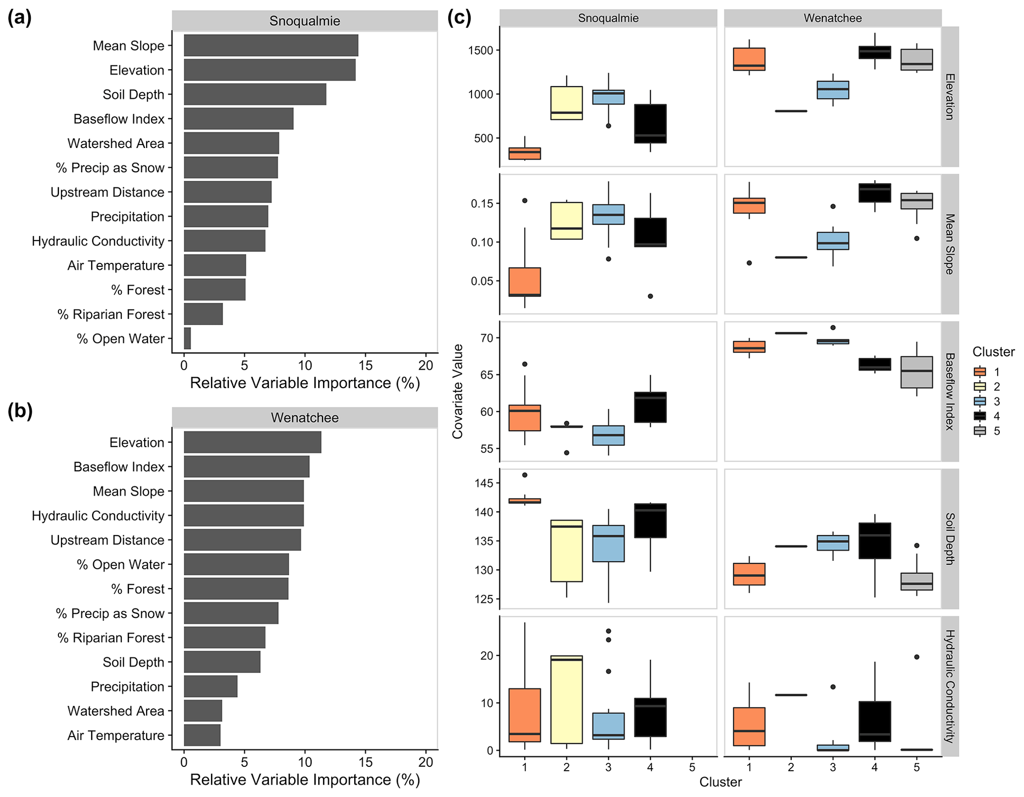
Figure 6 Relative variable importance for all covariates in the Snoqualmie (a) and Wenatchee (b) basins, together with the distributions of variables across clusters for the four most important variables (c) in the Snoqualmie basin (mean slope, elevation, soil depth, and baseflow index) and in the Wenatchee basin (elevation, baseflow index, mean slope, and hydraulic conductivity). Boxes are grouped and colored by cluster membership. See Fig. S8 for plots of the remaining relative variable importance.

4 Discussion

Thermal sensitivity varies throughout the year and reflects hydrologic conditions at a given time and place within a watershed; therefore, it should not be conceptualized as a static value. Although summary metrics of thermal sensitivity, such as average values over summer, can still prove useful and informative, it is essential to acknowledge the non-stationarity of the relationship between air and water temperature to obtain an accurate understanding of how river temperatures respond to changing conditions. We find that the underlying geology and climate are important controls on thermal sensitivity across two Pacific Northwest river basins, and thermal sensitivities reflect aspects of river dynamics not redundant with water and air temperature. Overall, this study provides a framework for using thermal sensitivity regimes to improve understanding of factors contributing to stream temperatures and will enable managers to target mitigation and adaptation activities to work best with local conditions within a watershed.

4.1 Patterns of thermal sensitivity clustering

Our analysis of stream air and water temperatures supports the presence of distinct thermal sensitivity regimes, providing an organizing framework for river research and management by identifying sites with similarities across the network. We found that thermal sensitivity regimes reflected non-redundant aspects of river dynamics relative to air and water temperature alone. Air temperature and water temperature clusters closely corresponded to one another and were almost entirely determined by the elevation of the temperature loggers, whereas thermal sensitivity clusters showed more variability in annual patterns and were intermixed spatially (Figs. 4 and 5). Previous studies within the Pacific Northwest found that, generally, colder streams are less sensitive to air temperature fluctuations than warmer streams (Luce et al., 2014; Kelleher et al., 2021). Air and water clustering results are consistent with previous studies that observed broad temporal correspondence of air and river temperature dynamics with differing magnitudes of response (Bower et al., 2004; Chu et al., 2010; Garner et al., 2014; Isaak et al., 2018b). More locally, Isaak et al. (2020) found that, across western rivers, much of the information in stream temperature records could be summarized by a relatively limited number of distinct regime components primarily driven by differences in elevation and latitude.

Viewing thermal sensitivity as a continuous parameter adds novel insights to our understanding of river basin functioning. Studies have highlighted the importance of annual shifts in the processes that drive heat budgets as well as the non-stationarity of the resulting statistical relationships (Arismendi et al., 2014; Boyer et al., 2021). Our clustering analysis overcomes these issues by using a varying coefficient model that treats thermal sensitivity as a continuous function through time rather than a series of discrete summary metrics, and it allows clustering based on the entirety of average annual patterns. The observed complexity in the thermal sensitivity response hints at the diversity of physical processes controlling the stream temperature response, and the large, clear shifts in the thermal sensitivity magnitude across the year call into question the common practice of summarizing a river's sensitivity as a static value. The ability to directly observe shifts in the air–water temperature relationships also opens the possibility of using thermal sensitivity as a diagnostic tool to examine gradual changes in the importance of drivers of water temperature, such as dynamic changes in riparian shading or snowmelt.

4.2 Climate controls on thermal sensitivity

Seasonal variability of thermal sensitivity metrics was evident for our basins. Within both the Snoqualmie and Wenatchee basins, winter thermal sensitivities were low and varied strongly with MWE (Fig. 1). Observed low thermal sensitivities in winter were likely due to the nonlinear relationship between air and stream temperature at cold temperatures when air temperatures can dip below the water temperature freezing limit (Mohseni et al., 1998, 1999). Air temperature covaries strongly with elevation in the Pacific Northwest basins, and sites that are high in the watershed will experience a greater number of sub-freezing days and therefore greater decoupling between air and water temperatures. Fall thermal sensitivities were relatively homogeneous, whereas spring and summer thermal sensitivities exhibited a broader range of values. We expect thermal sensitivities to be similar during periods of heavy precipitation, when water sources with thermal characteristics distinct from air temperature, such as groundwater and snowmelt, contribute relatively less flow. The greater variability of responses in spring and summer indicates that the relative magnitude of energy exchange processes controlling river temperatures are more diverse than in fall or winter (Hrachowitz et al., 2010).

Snowmelt likely contributed to observed differences in thermal sensitivity across sites in spring and early summer. For summary metrics, the relationship between snowmelt and spring thermal sensitivity formed a wedge-shaped pattern, wherein sites with limited snowmelt displayed both high and low thermal sensitivity, but sites with extensive snowmelt always display low thermal sensitivity (Fig. 3). For the clustering analysis, although the proportion of precipitation falling as snow showed limited variable importance, MWE and slope covaried closely with snow accumulation and were among the most important predictors of cluster membership, perhaps masking a statistical signal of snowfall (Fig. 6). In both the Snoqualmie and Wenatchee basins, clusters with higher elevation, steeper slopes, and greater snowmelt within the catchment had thermal regimes that were less sensitive to changes in air temperature during spring and early summer. Importantly, snowmelt buffering, the process wherein snowmelt-influenced streams have lower thermal sensitivity due to a direct input of cold water and a corresponding increase in flow rates and water depths (van Vliet et al., 2011; Siegel et al., 2022), diminishes throughout the summer. By late summer, high-elevation, snowmelt-influenced sites were often more sensitive to air temperatures than their low-elevation counterparts (Figs. 4 and 5). Sites within Cluster 4 in the Wenatchee basin were an exception to this pattern and maintained summer thermal sensitivities that were substantially depressed relative to adjacent locations (e.g., Clusters 1 and 5). This is likely due to continuous summer snowmelt inputs within these catchments and points to the importance of high-elevation, late-summer snowpack melt as a significant source of summer baseflow and control on water temperatures during the months of greatest heating within these watersheds.

Numerous studies have examined the buffering impact of snowmelt on water temperature due to advective flux from cooler meltwater entering the river. Studies in Alaskan rivers found a linear, negative relationship between summer thermal sensitivity and snowmelt (Lisi et al., 2015; Cline et al., 2020), and a recent study in the Snoqualmie basin found that snowmelt can reduce basin-wide peak summer temperatures, particularly in high-elevation tributaries, and the thermal impacts of meltwater can persist through the summer (Yan et al., 2021). Our results suggest that snowpack offers substantial buffering to changes in air temperature across mountain river basins but that the largest impacts are localized across space and time. Climate change is expected to shift snowmelt earlier and reduce snow water resources (Barnett et al., 2005; Musselman et al., 2021). The loss of snow may result in warming in snow-influenced systems and the subsequent homogenization of thermal conditions across basins (Winfree et al., 2018). Homogenization of thermal conditions likely leads to important changes in ecological functions and ecosystem services supported by lost thermal heterogeneity, such as a loss of cold-water patches for Pacific salmon (Brennan et al., 2019).

4.3 Hydrogeologic controls on thermal sensitivity

Hydrogeologic characteristics shaped the relationship between air and water temperatures across the Wenatchee and Snoqualmie basins. The inclusion of baseflow index, hydraulic conductivity, and soil depth in determining cluster membership (Fig. 6) implies the importance and detectability of groundwater as a key mediator of thermal sensitivity regimes in Pacific Northwest basins. Clusters with high baseflow index, hydraulic conductivity, and soil depth values generally had lower summer and less variable thermal sensitivities (Figs. 4, 5, and 6), implying greater groundwater influence (Kelleher et al., 2012). Interestingly, despite the clear importance of hydrogeologic metrics in the clustering analysis, results from summary metric exploratory analysis were mixed and, in the Snoqualmie basin, did not align with expectations of a negative relationship between thermal sensitivity and groundwater influence (Table 1b). Although it is possible to infer broad patterns in surface–groundwater connectivity using datasets of interpolated geologic properties (i.e., hydraulic conductivity, soil depth) or water sources (i.e., baseflow index), individual hydrogeologic metrics often have substantial uncertainty, do not covary perfectly, and may be particularly unconstrained for mountain headwater streams (Wolock et al., 2004; Patton et al., 2018; Briggs et al., 2022). Additionally, the influence of these processes can be localized and variable across space (Johnson et al., 2017) and substantially impacted by human modification. The ability to use thermal sensitivity as an empirical measure of groundwater influence, therefore, shows great promise for understanding catchment processes and informing management and restoration actions at ecologically relevant scales (Snyder et al., 2015). Although our approach moves us closer to a mechanistic understanding of the relationship between thermal sensitivity and groundwater, mixed results from our analyses emphasize the need for additional targeted studies.

An investigation of the underlying geology across the Snoqualmie and Wenatchee basins supports our conclusion that low thermal sensitivities are indicative of groundwater inputs. The lowland portion of the Snoqualmie watershed contains a deep, permeable, and productive glacial aquifer that is presumed to be the source of summer baseflow to much of the river (Bethel, 2004; McGill et al., 2021; Turney et al., 1995). Glacial and interglacial deposits in the valley contain several geohydrologic units with differing aquifer potentials (Bethel, 2004); however, most deposits can form small but useable aquifers that could help to sustain baseflow in summer months (Turney et al., 1995; Soulsby et al., 2004; Blumstock et al., 2015). Soil depth, hydraulic conductivity, and baseflow index were correspondingly high in streams from Clusters 1 and 4 that overlay the lower portion of the watershed (Fig. 6). Thermal sensitivities reflected this pattern, wherein sites draining low-elevation tributaries (Cluster 1) generally had relatively constant thermal sensitivities throughout the year (Fig. 4). Conversely, the upper portion of the Snoqualmie basin is covered by thin soil over impermeable bedrock lacking extensive fracture networks, meaning that rain and snowmelt are not retained in the mountains but are rapidly transmitted to the stream system (Debose and Klungland, 1964; Nelson, 1971; Goldin, 1973, 1992). Sites with catchments predominantly within this upland area tended to belong to Clusters 2 and 3 and displayed high summer thermal sensitivities, perhaps indicating limited groundwater buffering.

In the Wenatchee basin, two major aquifers exist: an aquifer within the sedimentary bedrock of the central and lowland areas and an overlying unconsolidated alluvial and outwash aquifer located primarily in river valley bottoms across the basin (Montgomery Water Group, 2003). The bedrock aquifer consists of sandstones and shales, which tend to have moderately low permeability. Folding and faulting have caused the shale to break up or fracture, and groundwater moves preferentially within these zones of higher secondary permeability. The alluvial and outwash aquifers, on the other hand, exhibit relatively high permeability where groundwater can move easily and are considered the primary groundwater source (Wildrick, 1979; Montgomery Water Group, 2003). Cluster 2 in the Wenatchee basin, consisting of a single site located at the mouth of Chumstick Creek (Fig. S5), stands out for having a unique, nearly flat thermal sensitivity compared to patterns at other sites (Fig. 5). Covariate distributions for the clustering results showed that Chumstick Creek has a relatively high hydraulic conductivity and baseflow index (Figs. 6 and S8). A transition from low- to high-permeability glacial material occurs near the mouth of Chumstick Creek (Montgomery Water Group, 2003), and it is possible that substantial groundwater discharge occurs near this discontinuity (Neff et al., 2019). Similarly, sites within Cluster 3 showed low variability in thermal sensitivity and had high soil depth and baseflow index values. Streams within this cluster are situated on top of predominantly sandstone bedrock (Frizzell, 1979; Gendaszek et al., 2014).

Overall, the importance of groundwater is consistent with previous studies, which find that thermal sensitivity decreased with increasing groundwater contribution (O'Driscoll and DeWalle, 2006; Chang and Psaris, 2013; Beaufort et al., 2020; Georges et al., 2021). The degree to which groundwater decouples trends in stream and air temperature depends on stream volume, the rate of groundwater inflow, and the depth of the groundwater source. Although not examined in this study, aquifer source and groundwater depth likely influence thermal sensitivity estimates, with runoff sourced from deep groundwater being less variable and less sensitive in comparison to groundwater sourced from shallow subsurface flows (Tague et al., 2007; Johnson et al., 2021; Hare et al., 2021). Shallow groundwater temperatures are already responding to climate change (Menberg et al., 2014). As warming continues, the summer cooling capacity of groundwater may be reduced, limiting the availability of cold-water refugia patches sourced by groundwater (Brewer, 2013; Briggs et al., 2013).

4.4 Landscape controls on thermal sensitivity

Variable relationships between thermal sensitivities and landscape covariates highlight complexities in stream thermal regimes. For example, mean channel slope was an important predictor of cluster membership for both the Snoqualmie and Wenatchee basins but showed a weak to non-existent relationship with summer thermal sensitivity summary metrics. Steeper channel slopes and greater stream velocities limit warming in streams by decreasing the time for equilibration with local heating conditions (Donato, 2002; Webb et al., 2008; Isaak et al., 2012), and topographic shading associated with steep watersheds can suppress stream temperature by reducing exposure to solar radiation (Webb and Zhang, 1997). In the Wenatchee basin, the Cluster 3 site, Chumstick Creek, drains a steep canyon. This may contribute to observed low, stable thermal sensitivities throughout the year. Additionally, watershed size and distance upstream covary closely and display relatively consistent relationships with summer thermal sensitivity summary metrics despite ranking moderately in variable importance. We expected thermal sensitivity to increase with river size; groundwater influence should be more visible in smaller streams because the volume of water is small and the travel time of the water from the source is short and not sufficient to equilibrate water temperature with the atmosphere (Mohseni and Stefan, 1999; Tague et al., 2007; Beaufort et al., 2016). Reduced sensitivity of headwater streams to air temperature was observed in the Aberdeenshire Dee, Scotland (Hrachowitz et al., 2010), and Danube River, Austria (Webb and Nobilis, 2007), and small Pennsylvanian streams were shown to be less sensitive to changes in air temperature than larger streams (Kelleher et al., 2012). However, Hilderbrand et al. (2014) found no relationship between thermal sensitivity and watershed size in Maryland streams.

We expected landscape covariates to be important predictors of thermal sensitivity regimes; however, these covariates were of limited importance and showed no relationship with summary metrics (Table 1b; Fig. 6). Several factors may account for this. Inherent covariation in river basins can hinder statistical efforts to identify mechanistic links between landscape gradients and features of aquatic ecosystems (Lucero et al., 2011); land cover characteristics may have a small impact that went undetected due to noisy observations or limited variability within our study region. It is also possible that land cover metrics may not adequately describe the intended process. For example, the relative unimportance of riparian shading may be due in part to our metric of shade, which was limited to riparian forest cover and ignored topographic shading and vegetation height. Lastly, human modifications to the river that are not captured by land cover statistics, such as channelization or the presence of dams and reservoirs, may alter thermal sensitivity and obscure natural gradients. For example, areas of the river that are degraded and subsequently disconnected from their floodplain may have artificially high thermal sensitivities, and the release of water from dams and reservoirs has the potential to either warm or cool downstream temperatures, depending on the dynamics of where and how impounded water is released (Ahmad et al., 2021; Cheng et al., 2022). Future research could include a covariate for sinuosity or variance of thalweg depth to better capture these effects. Untangling exact controls will require additional research.

4.5 Assessment of the statistical approach

Collecting data on dynamic stream networks over time has inherent challenges that lead to relatively low sample sizes and missing data as well as complex correlation structures across space and time. Our statistical approach was designed to manage these challenges, enabling exploration of several hypotheses. These data, collected at a relatively large number of sites in a parallel structure across two basins, allow an assessment of how sensitive the statistical approach may be to these constraints.

The time series of both air and water temperature used in this analysis have periods of missing values that span weeks to months. Classical clustering techniques require complete datasets, limiting analyses to time series without gaps. To overcome this issue, we calculated a single representative time series at each site that captures the typical range and timing of thermal sensitivity. Alternative options for dealing with missing values include removing data points that do not cover the target time period or imputing missing values by means of statistical procedures or summary metrics (e.g., Savoy et al., 2019; Beaufort et al., 2020). However, we chose not to use these approaches in our study due to the long and inconsistent periods of missing values across sites. We acknowledge that interannual variability in precipitation and temperature impacts river thermal sensitivity, and average time series calculated from differing years may exhibit differences in shape and timing for reasons outside of inherent characteristics (Sect. S1, “Interannual variability in thermal sensitivity”). Future studies could use novel clustering methods capable of dealing with sparse datasets, which would provide more detailed information on clusters generated from time periods with robust values versus data scarcity (Carro-Calvo et al., 2021). Alternatively, recent advances in space–time imputation for river basins may prove a fruitful direction (Li et al., 2017).

Our calculation of time-varying thermal sensitives also necessitated decisions regarding which features of the time series to preserve. Selection of the bandwidth parameter and kernel function for the time-varying model will impact estimation of the thermal sensitivity and intercept. Generally, with larger bandwidth estimates or averaging periods (e.g., daily, weekly, or monthly), intercept estimates increase and thermal sensitivity estimates decrease. Decisions of this nature should be approached carefully and with a clear question in mind. For this study, we were interested in seasonal to annual patterns in thermal sensitivity and thus chose a bandwidth of 0.2, resulting in a smooth seasonal time series. Previous studies have also used regression splines to estimate the time-varying relationship between air and water temperatures (Haggarty et al., 2015). This approach smooths data and can account for missing data but may not preserve small-scale features of interest. We chose to use absolute values of our thermal sensitivity time series, as we cared about differences in mean thermal sensitivity as well as correlated variability. Future work could normalize thermal sensitivity time series first to examine only patterns.

While general patterns could be detected through our analysis, the details were sensitive to exactly which sites were sampled and included in the analysis. In dynamic river systems with high spatial heterogeneity and inherent difficulties in accessing certain areas of the network, this is always likely to be true. Our approach of averaging across years and clustering across sites appears to manage these realities well and provide general guidance on the river networks sampled. For example, cross-validation results for CART modeling suggest that certain variables were consistently identified as more influential for cluster prediction and that results were relatively robust to the inclusion of individual data points (Fig. S7). Strengthening the assessment of underlying drivers and controls to provide guidance for unsampled river networks will require that similar datasets are collected across more and more river networks. Data can then be assembled and analyzed to provide more general conclusions about hydrogeologic, land use, and climatic controls of river thermal regimes.

4.6 Implications for management and future directions

Classifying rivers based on thermal sensitivity could be a powerful tool when planning for global change. Our results show that annual patterns in thermal sensitivity are diverse and mediated by the underlying geology and climate across two Pacific Northwest river basins. Climate change is decreasing snowpack in the region, resulting in earlier runoff and extended summer baseflow (Elsner et al., 2010; Wu et al., 2012), and may decrease groundwater discharge depending on the sources and timing of recharge (Brooks et al., 2012; McGill et al., 2021). For many of our study sites, thermal sensitives were highest in late summer during the hottest, lowest flow portion of the year. Previous studies have found that the impact of fluctuations in discharge generally increases during dry, warm periods, when rivers have a lower thermal capacity and are more sensitive to atmospheric warming (van Vliet et al., 2013). High thermal sensitivity in late summer and in high-elevation streams, which are typically thought to be climate refuges, is therefore troubling for the conservation of native cold-water species such as Pacific salmon (Mantua et al., 2010; Isaak et al., 2016). Climate change will likely decrease juvenile rearing and spawning habitat quantity and quality, although it is important to note that streams with high thermal sensitivity may still provide adequate habitat in selected portions of the year if stress-related thresholds are not exceeded (Armstrong et al., 2021).

Examining thermal sensitivity regimes improves understanding of factors contributing to stream temperatures and may enable managers to target mitigation and adaptation activities to work best with local conditions, thus maximizing benefits given limited resources. For example, given the importance of subsurface geology within the Wenatchee and Snoqualmie basins, targeted actions to restore floodplain functions that recharge aquifers through actions such as placing engineered logjams or reintroducing beavers could be prioritized (Abbe and Brooks, 2013; Pollock et al., 2014; Jordan and Fairfax, 2022). Additionally, identification of particularly insensitive portions of the river could help to better constrain areas where cold-water patches exist that may be used as refuges for cold-water fish (Snyder et al., 2020). This process-based approach will be particularly important as non-stationary relationships caused by climate change make it unreliable to use past regressions built under historical climate conditions (Boyer et al., 2021). Furthermore, as longer, more spatially extensive air and water temperature time series become available (Isaak et al., 2017), we can begin to ask questions about (1) the spatial extent of different thermal sensitivity regimes, (2) how interannual variability shifts with climate conditions and geographic context, and (3) detecting changes in the external drivers of thermal sensitivities. Such insights will improve our understanding of river ecosystems while offering a suite of new tools for monitoring the impact of management decisions and climate change.