Effects of high-quality elevation data and explanatory variables on the accuracy of flood inundation mapping via Height Above Nearest Drainage

Given the availability of high-quality and high-spatial-resolution digital elevation maps (DEMs) from the United States Geological Survey's 3D Elevation Program (3DEP), derived mostly from light detection and ranging (lidar) sensors, we examined the effects of these DEMs at various spatial resolutions on the quality of flood inundation map (FIM) extents derived from a terrain index known as Height Above Nearest Drainage (HAND). We found that using these DEMs improved the quality of resulting FIM extents at around 80 % of the catchments analyzed when compared to using DEMs from the National Hydrography Dataset Plus High Resolution (NHDPlusHR) program. Additionally, we varied the spatial resolution of the 3DEP DEMs at 3, 5, 10, 15, and 20 m (meters), and the results showed no significant overall effect on FIM extent quality across resolutions. However, further analysis at coarser resolutions of 60 and 90 m revealed a significant degradation in FIM skill, highlighting the limitations of using extremely coarse-resolution DEMs. Our experiments demonstrated a significant burden in terms of the computational time required to produce HAND and related data at finer resolutions. We fit a multiple linear regression model to help explain catchment-scale variations in the four metrics employed and found that the lack of reservoir flooding or inundation upstream of river retention systems was a significant factor in our analysis. For validation, we used Interagency Flood Risk Management (InFRM) Base Level Engineering (BLE)-produced FIM extents and streamflows at the 100- and 500-year event magnitudes in a sub-region in eastern Texas.

1 Introduction

Floods are among the most frequent, damaging, and deadly of natural disasters (Doocy et al., 2013; Strömberg, 2007; Kahn, 2005). The frequency and intensity of flood events, as well as the exposure of people and property to them, have been increasing in recent times, driven by secular changes in climate, infrastructure, and demographics (Berz, 2000; Mallakpour and Villarini, 2015; Downton et al., 2005; Kunkel et al., 1999; Pielke and Downton, 2000; Corringham and Cayan, 2019; Gourevitch et al., 2023). These upward trends are expected to continue placing additional pressure on hydrological extremes (Kahn, 2005; Tabari, 2020; Milly et al., 2002; Wing et al., 2018; Gourevitch et al., 2023). Floods impact mortality and morbidity through drowning or physical trauma at the individual-health scale while increasing the risk of infectious disease at the public-health level (Jonkman, 2005; Beinin, 2012; Alajo et al., 2006; French et al., 1983). Flooding disrupts systems that provide for human needs such as transportation routes, supply chains, water delivery, waste management, communications, shelter, and energy grids (Wijkman and Timberlake, 2021; Gourevitch et al., 2023). These impacts disproportionately affect certain demographics such as the socioeconomically disadvantaged, youth, and elderly, who are more likely to live in vulnerable areas with less access to educational resources, early-warning systems, and the capacity or resources to evacuate impacted areas (Kahn, 2005; Smiley et al., 2022; Strömberg, 2007; Jonkman, 2005; Tellman et al., 2020, 2021). These inequitable impacts further entrench poverty and inequalities (Stallings, 1988; Birkmann et al., 2010). In political terms, severe disasters, including floods, can reduce social order, strain governance systems, collapse social safety nets, and increase the risk of social conflict (Drury and Olson, 1998; Xu et al., 2016; Zahran et al., 2009). These dire consequences motivate adaption and mitigation efforts such as early-warning systems, protective infrastructure (e.g., storage, defenses, drainage, infiltration), public awareness and education, and zoning regulations (Tumbare, 2000; Tauhid and Zawani, 2018; Charlesworth and Warwick, 2011).

Due to these growing flood risks, early-warning systems or forecasting systems can help in understanding future conditions and can provide intelligence to furnish adequate warnings to protect life, prevent damage, and enhance resilience (Strömberg, 2007; Cools et al., 2016; UNISDR, 2015; Baudoin et al., 2014; Golnaraghi, 2012; UNEP, 2012; C. Liu et al., 2018; Schumann et al., 2013). The early warning of flood disasters at national scales often requires the use of continental-scale forecast hydrology models and modeling frameworks that span intranational political boundaries. The applications of these models extend beyond early-warning systems to providing historical trends for applications in infrastructure planning, public planning, insurance underwriting, and more. The Office of Water Prediction (OWP), an office of the National Oceanic and Atmospheric Administration (NOAA), along with partners at the National Center for Atmospheric Research (NCAR), developed such a continental-scale model known as the United States (US) National Water Model (NWM) (Salas et al., 2018; Gochis et al., 2021; Cosgrove et al., 2019; Cohen et al., 2018; NOAA, 2016; Office of Water Prediction, 2022). The NWM is based on a configuration of the Weather Research and Forecasting Hydro (WRF-Hydro) model that accounts for land surface processes, as well as overland and channel routing (Gochis et al., 2021; Salas et al., 2018; Cosgrove et al., 2019). Operationally, the NWM produces streamflow analysis and forecasts at multiple time horizons depending on location, which includes the conterminous US (CONUS), Puerto Rico, Hawaii, and portions of Alaska (Cosgrove et al., 2019; NOAA, 2016; Office of Water Prediction, 2022). The NWM routes streamflow across the NWM Version 2.1 (V2.1) stream network, which is based on the National Hydrography Dataset Plus Version 2 (NHDPlusV2) network and is comprised of more than 5.5×10⁶ km (kilometers) of lines discretized into more than 2.8 million forecast points (Aristizabal et al., 2023c). The NWM V2.1 stream network belongs to the NWM “hydrofabric”, defined as a catalog of geospatial layers relevant to hydrology modeling, including stream network flow paths, catchments, reservoirs, and more (Office of Water Prediction, 2022; Cosgrove et al., 2019). While streamflow is an important variable for engineering and scientific applications of fluvial flooding, flood inundation stages, extents, and depths are much more tangible variables to the stakeholders that flood events directly impact.

The shallow-water equations, a system of two hyperbolic partial differential equations, formally govern the flow of fluvial surface water by conserving both mass (first equation) and momentum (second equation) and can be expressed in both one-dimensional (1D) (Saint-Venant equations) and two-dimensional (2D) forms. Solving this system in full 2D form requires numerical methods that can be very cost prohibitive and numerically unstable in an operational setting across continental scales at high spatial discretizations (10 m (meters) or higher). This use case motivates the implementation of an inundation proxy, also known as a zero-physics or simplified conceptual model, that is agnostic to the shallow-water equations while still computing accurate fluvial inundation extents and depths (Teng et al., 2015; Bates and De Roo, 2000). Height Above Nearest Drainage (HAND) de-trends elevations within digital elevation models (DEMs) to compute drainage potentials by normalizing elevations to the nearest relevant flow path instead of data that represent mean sea level (Rennó et al., 2008; Nobre et al., 2011, 2016). HAND, as a terrain index, has been used extensively for producing flood inundation maps (FIMs) from both modeled or observed streamflows and stages (Nobre et al., 2016; Afshari et al., 2018; Garousi-Nejad et al., 2019; Johnson et al., 2019; Zheng et al., 2018a, b; Zhang et al., 2018; Teng et al., 2015; Li et al., 2022), as well as for assisting in the remote sensing detection of fluvial inundation (Aristizabal et al., 2020; Shastry et al., 2019; Aristizabal and Judge, 2021; Huang et al., 2017; Twele et al., 2016). HAND operates as an inundation proxy by thresholding the relative elevation (or HAND) values with a singular river stage value for each catchment, corresponding to the drainage area of a given river reach (Nobre et al., 2016; Garousi-Nejad et al., 2019; Johnson et al., 2019; Zheng et al., 2018a; Teng et al., 2015; Liu et al., 2016; Maidment, 2017; Y. Y. Liu et al., 2018; Liu et al., 2020; C. Liu et al., 2018). When used to generate inundation extents and depths from streamflow, reach-averaged synthetic rating curves (SRCs) sample geometric variables along an entire reach and normalize these using the length of the reach to create stage–discharge relationships (Zheng et al., 2018b; Aristizabal et al., 2023c; Godbout et al., 2019). These relationships depend on the friction parameter, Manning's n, and are used to convert streamflows to stages for eventual 2D mapping with HAND. Numerous investigations have validated the use of HAND for flood-mapping applications as a suitable alternative to more sophisticated physics-based techniques for large-scale and high-resolution use cases (Johnson et al., 2019; Li et al., 2023; Aristizabal et al., 2023c; Nobre et al., 2016; Godbout et al., 2019; Afshari et al., 2018; Zhang et al., 2018; Teng et al., 2015, 2017; Diehl et al., 2021; Hocini et al., 2021; Bates et al., 2003).

Several prior and active large-scale HAND implementations catered to operational early-warning-system applications, including the National Flood Interoperability Experiment (NFIE) (Maidment, 2017; Liu et al., 2016; Y. Y. Liu et al., 2018), GeoFlood (Zheng et al., 2018a; Hocini et al., 2021; D'Angelo et al., 2022; Carruthers, 2021; Zheng et al., 2022), and PyGFT (Petrochenkov and Viger, 2020; Verdin et al., 2016). The NFIE was a broad, inter-institutional, and pioneering effort to apply HAND to the initial versions of the NWM, which leveraged $\mathrm{1}/\mathrm{3}$ arcsec (10 m) seamless elevation data available at the time (Maidment, 2017; Liu et al., 2016; Y. Y. Liu et al., 2018) from the USGS's National Elevation Dataset (NED) (Gesch et al., 2002; Gesch and Maune, 2007). Zheng et al. (2018a) applied HAND to operational applications with $\mathrm{1}/\mathrm{27}$ arcsec (1 m) elevation data with a novel least-cost, geodesic-based stream delineation method (Passalacqua et al., 2010, 2012; Zheng et al., 2018a, 2019; Carruthers, 2021; D'Angelo et al., 2022; Zheng et al., 2022). For applications with the NWM, an advanced version of HAND coupled with the use of SRCs, known as OWP FIM, converts NWM analysis, reanalysis, and forecast streamflows to river stages and operationally based fluvial inundation depths and extents to CONUS while extending the modeling domain to Puerto Rico and Hawaii (Aristizabal et al., 2023c, b). OWP FIM utilizes some of the latest datasets, including the National Hydrography Dataset Plus High Resolution (NHDPlusHR) (Moore et al., 2019), the National Levee Database (NLD) (US Army Corps of Engineers, 2021), and the NWM V2.1 hydrofabric (Office of Water Prediction, 2022; NOAA, 2016; OWP/ESIP, 2021; Gochis et al., 2021). These datasets enforce hydrologically relevant features such as levees and the general location of flow paths to facilitate conflation with the forecast stream network (Aristizabal et al., 2023c, b). Additionally, OWP FIM advanced a fundamental limitation of HAND that limits sourcing fluvial inundation to be from only the nearest relevant flow path (McGehee et al., 2016; Aristizabal et al., 2023c; Zhang et al., 2018; Li et al., 2023; Zheng et al., 2018a, b; Nobre et al., 2016). Flow paths of higher Horton–Strahler stream order that could contribute inundation to a given area have no way of extending beyond catchment lines, which creates artificial bottlenecks in inundation extents, especially along junctions of high-order rivers with their lower-flow tributaries (Aristizabal et al., 2023c; McGehee et al., 2016). To resolve this limitation, OWP FIM disaggregates the NWM V2.1 stream network into segments of effective unit stream order referred to as level paths in a version of HAND called Generalized Mainstems (GMS) (Aristizabal et al., 2023c). In terms of terrain data, OWP FIM uses the 10 m DEM from the NHDPlusHR elevation dataset, which is the elevation basis, derived in batches from the 3D Elevation Program (3DEP), for additional hydrography products within the NHDPlusHR (Aristizabal et al., 2023c; Moore et al., 2019). The previous advances in OWP FIM stopped short of accounting for light detection and ranging (lidar) point elevation observations (Aristizabal et al., 2023c) that are now nearing their first collection cycle to form a novel, seamless, continental-scale DEM from 3DEP (USGS, 2021b, 2022a).

Broad-scale terrain information in the form of DEMs is fundamental to all FIM models and has a significant influence on inundation skill (Bales and Wagner, 2009; Dobbs, 2010; Wang and Zheng, 2005; Merwade et al., 2008; Witt, 2015; Garousi-Nejad et al., 2019; Li et al., 2022; Neal et al., 2011). The National Geospatial Program, under the USGS, is the primary authority on collecting, processing, and maintaining terrestrial elevation data within the US in collaboration with federal partners within the National Digital Elevation Program (NDEP) (Office of Management and Budget, 2016; Dewberry, 2011; National Research Council, 2007, 2009; Sugarbaker et al., 2014). The NED (Gesch et al., 2002; Gesch and Maune, 2007) forms the seamless elevation layers of The National Map (TNM) (Gesch et al., 2009; Archuleta et al., 2017; S. Arundel et al., 2015; Arundel et al., 2018; Kelmelis et al., 2003). Prior to the introduction of 3DEP, TNM was originally composed of three seamless DEMs at $\mathrm{1}/\mathrm{3}$ (10 m), 1 (30 m), and 2 (90 m) arcsec resolutions produced from a variety of legacy sources including digital photogrammetry, cartographic contours, mapped hydrography, and elevations from the Shuttle Radar Topography Mission (SRTM) (Gesch et al., 2002; Gesch and Maune, 2007; S. Arundel et al., 2015). High-quality elevations derived from lidar and interferometric synthetic aperture radar (InSAR) have been integrated into TNM seamless elevation products, as made available prior to and after the introduction of 3DEP (Snyder et al., 2013; Gesch et al., 2002; S. Arundel et al., 2015). Work by Gesch et al. (2014), Gesch and Maune (2007), and Dobbs (2010) illustrated that the inclusion of higher-quality elevation data sources brought about a significant improvement in the accuracy of NED data when compared to the National Geodetic Survey (NGS) (Roman et al., 2010). Gesch et al. (2014) identified that the NED $\mathrm{1}/\mathrm{3}$ arcsec DEM, as of April 2013, had a mean error of −0.29 m, with a root mean squared error (RMSE) of 1.55 m, when compared to over 25 000 reference points. At the time of evaluation, the NED was subject to legacy, lower-quality data sources dating back almost a century in the past (Sugarbaker et al., 2014; Gesch et al., 2014; Gesch and Maune, 2007). This reduction in error and its impact on people and commerce (Dewberry, 2011) motivated action on the collection of elevation data from higher-quality data sources (Sugarbaker et al., 2014).

The 3DEP is a national, multi-organizational effort by the NDEP to survey elevations with high-quality sensors on a recurring collection cycle of no more than 8 years in response to growing stakeholder needs (Dewberry, 2011; Snyder et al., 2013; Sugarbaker et al., 2014). The 3DEP leverages two main collection technologies, including lidar for the CONUS, Hawaii, and US territories and InSAR for Alaska. The lidar, the collection source of focus in this study, is a light emission, reflection, and collection technology that beams concentrated, powerful light of wavelengths between 1000–1600 nm (nanometers) (Muhadi et al., 2020). The reflection of the light is collected while recording the travel time and intensity of return; lidar sensors are mounted on top of a variety of mobile or static platforms whose positions are geo-tracked as they collect lidar returns (Passalacqua et al., 2015). The travel time of the returns, along with knowledge of the speed of light, serves as a relative positioning of the target(s) referenced to a common vertical datum, while the intensities serve as indicators of what the target(s) represents. Modes within the relationship of return intensities with respect to travel time or distance from the lidar wave forms can be indicative of vegetation or other land uses and land covers (LULCs) that reflect signals at varying distances and magnitudes and influence elevation errors (Gesch et al., 2014). These modes can be discretized into varying DEM products representing bare earth, structures, or canopy elevations. The horizontal and vertical accuracies and the horizontal resolutions of terrain observations derived from lidar, and even the consequential economic benefits (Dewberry, 2011, 2022), are dependent on a variety of sensor, platform, target, and collection specifications and practices, such as nominal pulse spacing, nominal pulse density, and the LULC of the target (Heidemann, 2018; Passalacqua et al., 2015; Smith et al., 2019; Salach et al., 2018; Gesch et al., 2014). The lidar produces point cloud datasets, which are scattered, geo-referenced points representing full wave forms or discretized return intensities. Various assessments of the vertical accuracies of lidar point clouds have yielded satisfactory results in agreement with 3DEP requirements (Stoker and Miller, 2022; Kim et al., 2022; Callahan and Berber, 2022; Kim et al., 2022; Salach et al., 2018; Passalacqua et al., 2015). Point clouds must undergo a series of operations to produce analysis-ready, seamless DEMs (Passalacqua et al., 2015).

The 3DEP extends TNM to include a $\mathrm{1}/\mathrm{27}$ arcsec (1 m), lidar-derived DEM product for CONUS, Hawaii, and US territories, as well as a $\mathrm{1}/\mathrm{2}$ arcsec (5 m) DEM derived from InSAR for Alaska (Sugarbaker et al., 2014; Stoker et al., 2015). To create bare-earth DEMs, lidar observations must undergo a series of processes that filter out returns from vegetation, anthropogenic, and other features and then grid the observations with resampling methods (Passalacqua et al., 2015). The 1 m 3DEP product is a hydrologically flattened, topographic, and bare-earth raster DEM gridded to 1 km square-shaped tiles with 6 pixels of overlap (S. T. Arundel et al., 2015). Hydro-flattening refers to a process in which hydrologic features such as lakes, reservoirs, streams, rivers, and more are flattened in elevation for bathymetric regions from lower bank to lower bank, as represented by break lines (Archuleta et al., 2017; Maune and Nayegandhi, 2018). This flattening excludes along-gradient directions, parallel to the direction of the break lines, for hydrologic features that naturally exhibit water conveyance such as streams, rivers, and long reservoirs (S. T. Arundel et al., 2015). This process includes elevations underneath bridges that are not accurately observed by topographic lidar (Bales and Wagner, 2009). According to specifications, the horizontal accuracy of the 1 m 3DEP is within 1 m, while the vertical accuracies are within 19.6 and 30 cm (centimeters) at the 95 % confidence interval for non-vegetative and vegetative regions, respectively (S. T. Arundel et al., 2015; Heidemann, 2018). Non-vegetative vertical accuracies fall within an RMSE of 10 cm (S. T. Arundel et al., 2015; Heidemann, 2018). Work by Stoker and Miller (2022), Callahan and Berber (2022), and Kim et al. (2022) has verified the vertical accuracies and general quality of the DEMs for 3DEP specifications.

The quality of FIM extents is subject to a wide variety of terrain-related factors including collection technology, gridding methods, resampling techniques, hydrological conditioning processes, presence of bathymetry, vertical accuracies, and horizontal resolutions (Merwade et al., 2008). The main enhancement of including 3DEP data within HAND-based OWP FIM is the broader availability of high-quality data sources for elevations, such as lidar with enhanced vertical accuracies and horizontal resolutions (S. T. Arundel et al., 2015; Stoker and Miller, 2022; Archuleta et al., 2017). Generally speaking, with regard to the quality of FIM extents, the literature has demonstrated the sensitivity to, and improved effect of, using 3DEP or lidar data, mostly due to the enhanced vertical accuracies that these data sources provide (Podhorányi and Fedorcak, 2015; Bales and Wagner, 2009; Merwade et al., 2008; Witt, 2015; Mason et al., 2007; Zheng et al., 2018a). Limitations have been noted with respect to vertical accuracies in areas with vegetation, buildings, or bridges and/or areas that have been classified as bathymetric (Merwade et al., 2008; Mason et al., 2007; Bales and Wagner, 2009; Podhorányi and Fedorcak, 2015). FIM extents in areas of low topographic relief or areas behind natural or anthropogenic flow divides can be very sensitive to vertical accuracies (Sanyal and Lu, 2004; Garousi-Nejad et al., 2019; Godbout et al., 2019; Jafarzadegan and Merwade, 2017; Papaioannou et al., 2017). Specifically for HAND, research by Zheng et al. (2018a) and Garousi-Nejad et al. (2019) noted improvement when utilizing higher-resolution lidar-derived DEMs for HAND-based FIM.

The spatial resolution of topography likely interacts with many other sources of FIM extent uncertainties, including but not limited to elevation source quality, LULC, streamflow intensities, physics employed, and model parameterizations (Fewtrell et al., 2008; Savage et al., 2016; Neal et al., 2011; Thomas Steven Savage et al., 2016). Numerous researchers have evaluated resolution more generally across the spectrum of FIM models to focus more on urban areas where resolution could play an integral part in determining extents (Fewtrell et al., 2008; Neal et al., 2011; Ozdemir et al., 2013; Muthusamy et al., 2021; Savage et al., 2016; de Almeida et al., 2018; Dixon and Earls, 2009). While the studies evaluating HAND are extensive (Afshari et al., 2018; Nobre et al., 2011; Garousi-Nejad et al., 2019; Godbout et al., 2019; Speckhann et al., 2018; McGrath et al., 2018; McGehee et al., 2016; Li et al., 2020, 2022, 2023; Liu et al., 2016; Y. Y. Liu et al., 2018; C. Liu et al., 2018; Li and Demir, 2022; Liu et al., 2020; Aristizabal et al., 2023c; Maidment, 2017; Zheng et al., 2018a, b, 2019; Diehl et al., 2021; Johnson et al., 2019; Jafarzadegan and Merwade, 2019), only a few studies have investigated the effects of high-quality DEMs and their spatial resolutions on FIM extents when derived from HAND. Li et al. (2022) evaluated HAND-based FIM over a small domain and concluded that resampled lidar performed best at the 5 m spatial resolution when compared to coarser, resampled grids. Zheng et al. (2018a) incorporated lidar-derived elevations while also incorporating a novel stream delineation method and concluded that both combined performed better than utilizing legacy NED 10 m datasets with NHDPlusV2 hydrography as the data for HAND computation. Lastly, working in flat areas with some anthropogenic influence, Garousi-Nejad et al. (2019) used a 3 m DEM and found improvement in FIM quality extents when compared to the use of a 10 m DEM derived from different sources. In contrast to the other studies, Speckhann et al. (2018) evaluated the sensitivity of HAND-based FIM extents to DEM resolution in Brazil using DEMs from SRTM and found little to no effect in this region. Both Garousi-Nejad et al. (2019) and Zheng et al. (2018a) highlighted the importance of high-resolution elevations and novel stream delineation tools to avoid the negative effects of little to no bathymetric information. Due to the interacting uncertainties and the dearth of research on this question with respect to HAND, it is difficult to conclude what the effect would be on the quality of HAND-based OWP FIM of incorporating the latest 3DEP data at varying spatial resolutions.

As the spatial coverage of the 3DEP 1 m product rapidly approaches the CONUS scale in 2023, we investigate the integration of 3DEP data into OWP FIM for model-specific evaluation (USGS, 2021b, 2022a). We use 3DEP data for the HAND computation process to generate the FIM hydrofabric. OWP FIM uses a novel combination of input datasets, hydrological conditioning (hydro-conditioning) processes, level-path-scale processing, and parameterizations to produce HAND, and these specific combinations of methods could interact with terrain-related variables including source and resolution. Additionally, we investigated the utility of varying spatial resolutions at 3, 5, 10, 15, and 20 m, specifically its effect on FIM extents. HAND depends on the drainage assumptions which require DEMs to undergo a long series of enforcement processes to ensure monotonically decreasing elevations with hydrologically correct flow directions (Garousi-Nejad et al., 2019; Nobre et al., 2011, 2016; Aristizabal et al., 2023c). The resampling of DEMs into varying spatial resolutions could interact with these hydro-conditioning operations, thus influencing the FIM hydrofabric and the resulting quality of the FIMs produced. OWP FIM is scheduled for public release in 2023 for a region covering 10 % of the US population. Evaluations are needed specifically for this region and of how 3DEP elevations at varying resolutions affect skill. As validation, we used the 1D Hydrologic Engineering Center River Analysis System (HEC-RAS)-modeled flood inundation extents from the Base Level Engineering (BLE) published by the Interagency Flood Risk Management (InFRM) team. By varying the spatial resolution of 3DEP DEMs, we seek to quantify in an empirical fashion the relationship between the spatial resolution and FIM skill produced from HAND; this requires significant DEM manipulations to satisfy inherent assumptions. For analysis purposes, we consider a series of potential, catchment-scale explanatory variables with multi-variable regression analysis to help explain some of the catchment-scale variation in the metrics we employed to describe agreement with the BLE FIMs.

2 Materials and methods

2.1 Overview

Investigating the effects of lidar-derived DEMs and their spatial resolutions involved a multi-step process of data curation, production, evaluation, and analysis. Source information was gathered to produce HAND and its associated datasets, most specifically the DEMs, from multiple sources and spatial resolutions, including 3, 5, 10, 15, and 20 m. Later in the analysis, the resolutions of 60 and 90 m were assessed to help identify if and when spatial resolution begins to influence FIM quality. The FIM hydrofabric, or the collection of datasets required to convert streamflows to FIM extents, was produced using these various DEMs (Aristizabal et al., 2023c; Aristizabal and Judge, 2021). FIMs were produced by intersecting the BLE cross-sections, as described by Aristizabal et al. (2023c), furnished by the InFRM team for both the 1 % (100-year) and 0.2 % (500-year) recurrence flows (FEMA, 2016, 2021a, b; Strategic Alliance for Risk Reduction II, 2019a, b, c, d, e, f, g). These intersected flows were converted to reach-averaged stages using SRCs (Aristizabal et al., 2023c; Liu et al., 2016; Y. Y. Liu et al., 2018; Zheng et al., 2018b). Reach-averaged stages were used to threshold HAND values on a per-catchment basis, which translates to a flooded pixel when the stage value exceeds zero (Zheng et al., 2018b; Aristizabal et al., 2023c). Catchments are defined here as the unique surface drainage areas assigned to each river reach. These extents at the 100- and 500-year flow magnitudes were then compared to the original BLE-furnished extents for the corresponding magnitudes. Agreement statistics and maps were computed for binary categorical variables (inundated indicates positive and not inundated indicates negative) and then were resampled to the catchment scale. A number of covariates and factors were selected at the catchment scale for analysis purposes to explain some of the catchment-to-catchment variance in the selected metrics with the help of regression models. A high-level graphical summary of this explanation is presented in Fig. 1.

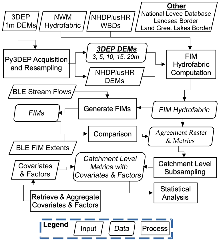
Figure 1 This figure illustrates the overall process for generating Height Above Nearest Drainage (HAND) and evaluating the use of light detection and ranging (lidar)-derived digital elevation models (DEMs) and their resolutions. Input datasets were collected from two different source DEMs, the 3D Elevation Program (3DEP) and the National Hydrography Dataset Plus High Resolution (NHDPlusHR). The 3DEP DEMs were resampled with the Python 3D Elevation Program (Py3DEP) to 3, 5, 10, 15, and 20 m spatial resolutions. Both source DEMs and their resolutions were used to compute the flood inundation map (FIM) hydrofabric, which is comprised of various datasets used to produce FIM, including HAND, catchments, and synthetic rating curves (SRCs). Base Level Engineering (BLE) cross-sections were intersected with the National Water Model (NWM) stream network to obtain streamflow estimates. These estimates were used to produce FIM using the SRC coupled with HAND to produce estimates of the 100- and 500-year extents. These extents were then compared to the extents from the BLE, thus removing hydrology-related errors that could be introduced if NWM streamflows were used. The agreement statistics were resampled to the NWM catchment level and then were referenced to a long series of catchment-level covariates and factors that were used for statistical analysis and inference.

2.2 Datasets

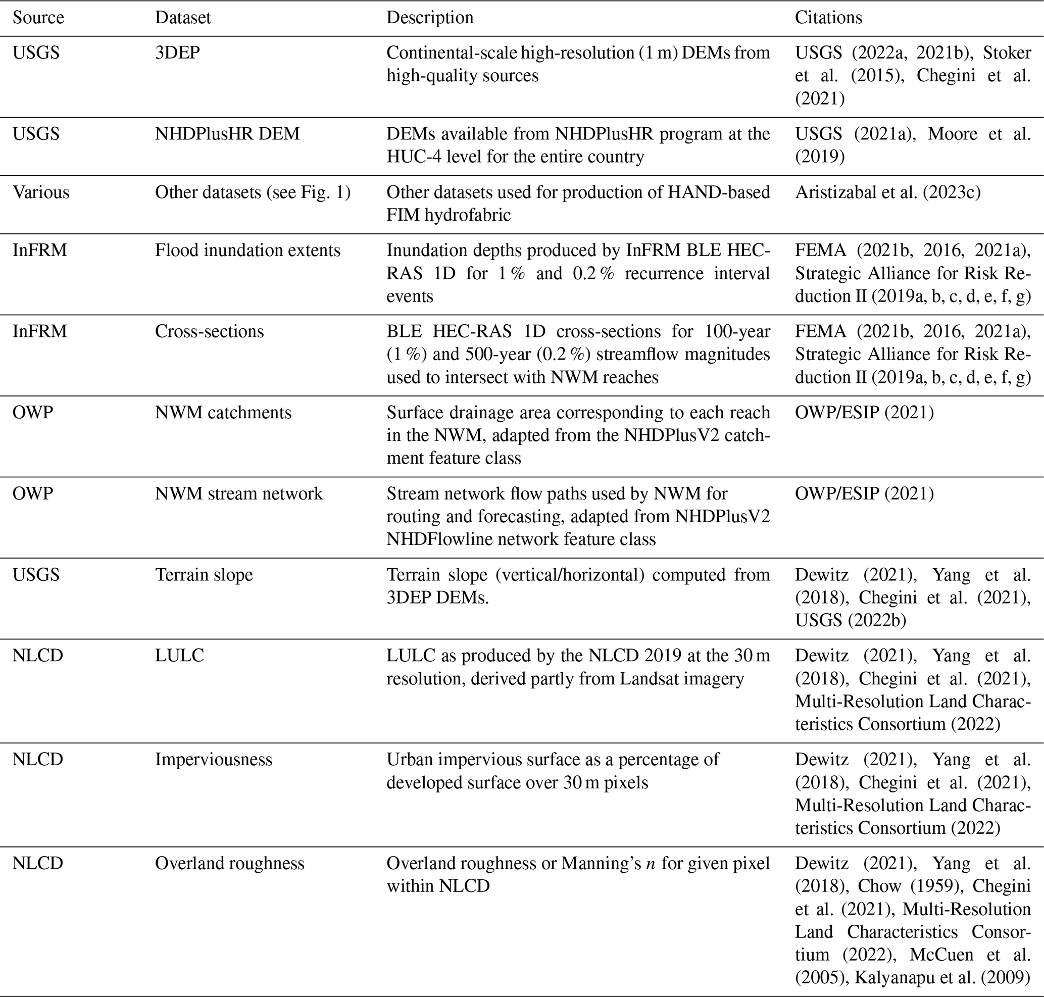
We used a wide variety of datasets for investigating the effects of DEM source and spatial resolution on FIMs produced from HAND. We compared legacy DEMs, used by Aristizabal et al. (2023c) and sourced from the NHDPlusHR program, that were available for the entire NWM domain at the hydrologic unit code (HUC)-4 scale. As the 3DEP program rapidly approaches continental-scale availability, the inclusion of 3DEP DEMs was considered here at various spatial resolutions (USGS, 2022a; Stoker et al., 2015; USGS, 2021b; Chegini et al., 2021; USGS, 2022b). Aristizabal et al. (2023c) provided more details for the datasets listed in Fig. 1, as denoted by “Other”. The remaining datasets used in this study for DEM experimentation and for analysis are elaborated on in Table 1. The analysis datasets are those used to help explain some of the spatial variation in the metrics. NWM catchments were used to resample the agreement maps and metrics down to the catchment scale. Analyses of the importance of various attributes within NWM catchments considered flow path properties such as channel slope, length, presence of reservoirs, and catchment area. Other attributes, aggregated to the catchment scale for consideration, included terrain slope, imperviousness, overland roughness, and LULC from the National Land Cover Database (NLCD), which were used as either covariates or factors in the statistical analysis of this study.

USGS (2022a, 2021b)Stoker et al. (2015)Chegini et al. (2021)USGS (2021a)Moore et al. (2019)Aristizabal et al. (2023c)FEMA (2021b, a, 2016)Strategic Alliance for Risk Reduction II (2019a, b, c, d, e, f, g)FEMA (2021b, a, 2016)Strategic Alliance for Risk Reduction II (2019a, b, c, d, e, f, g)OWP/ESIP (2021)OWP/ESIP (2021)Dewitz (2021)Yang et al. (2018)Chegini et al. (2021)USGS (2022b)Dewitz (2021)Yang et al. (2018)Chegini et al. (2021)Multi-Resolution Land Characteristics Consortium (2022)Dewitz (2021)Yang et al. (2018)Chegini et al. (2021)Multi-Resolution Land Characteristics Consortium (2022)Dewitz (2021)Yang et al. (2018)Chow (1959)Chegini et al. (2021)Multi-Resolution Land Characteristics Consortium (2022)McCuen et al. (2005)Kalyanapu et al. (2009)

Table 1 Dataset sources, names, descriptions, and citations. Datasets used to generate Height Above Nearest Drainage (HAND), except for the digital elevation model (DEMs), are not listed in detail here but are explained by Aristizabal et al. (2023c).

2.3 Data retrieval

We used the Hydroclimate Data Retriever (HyRiver) (Chegini et al., 2021) for retrieving topographic, LULC, imperviousness, and overland roughness data. HyRiver is a suite of nine open-source Python packages that provide access to a wide variety of hydrology and climatology datasets within the US through web services. In this study, we used two of these packages: the Python 3D Elevation Program (Py3DEP) and Python Hydrogeological (PyGeoHydro) datasets.

Py3DEP provides access to 3DEP's dynamic and static services. The dynamic service retrieves topographic data at any resolution using the best available raw elevation data for a requested region, whereas the static service only provides DEM data at 10, 30, and 60 m resolutions. It has some other utilities, including querying the availability of raw elevation data at different resolutions from various sources. In this study, we used the dynamic service to obtain DEMs at different resolutions and the raw data availability functionality of Py3DEP for determining the highest-resolution data available in the region of our study.

While Py3DEP is developed only for retrieving topographic data from a single source, PyGeoHydro can query various types of data from different sources, e.g., the National Inventory of Dams (United States Army Corps of Engineers, 2023), the Watershed Boundary Dataset (United States Geological Survey, 2023), and the National Land Cover Database (Multi-Resolution Land Characteristics Consortium, 2022). It also includes additional functionalities, including a look-up table for associating overland roughness to land cover type based on Liu et al. (2019). In this study, we obtained HUC geometries, reservoirs, LULC, imperviousness, and overland roughness data using PyGeoHydro.

2.4 DEM preparation

DEMs underwent a curation procedure prior to use with HAND computation and our experimental design. To match the existing framework with the use of NHDPlusHR DEMs, Py3DEP was used to query the image server to acquire 3DEP elevations at an HUC-4 scale. To counter pixel limitations within the web service, queries were completed using overlapping tiles and were mosaicked together using virtual rasters (VRTs) (USGS, 2022b). To investigate the effect of varying spatial resolutions on FIM skill and computational performance, queries were elected to be taken at 3, 5, 10, 15, and 20 m spatial resolutions. As stated previously, the resolutions of 60 and 90 m were also used to help understand if and when spatial resolution begins to affect quality. Utilizing the check_3dep_availability tool, we determined that 1 m 3DEP information is available for the entire study region (see Sect. 2.5). Py3DEP queries a US Geological Survey (USGS) dynamic web service for the best available DEM when generating its mosaics and resamples them given the user-furnished resolution (USGS, 2022b). Use of the Py3DEP function query_3dep_source confirmed availability of 1 m lidar data for the entire study area, which means the functionality uses it for resampling purposes (Chegini et al., 2021; Stoker et al., 2015; USGS, 2022b, a, 2021b). The availability of the 1 m data and of the other available source DEMs is illustrated in Fig. 2. The selected resolutions of 3, 5, 10, 15, and 20 m were bounded by computational demands since further optimizations within the code and external dependencies should be considered prior to transitioning to 1 m elevation information for HAND computation.

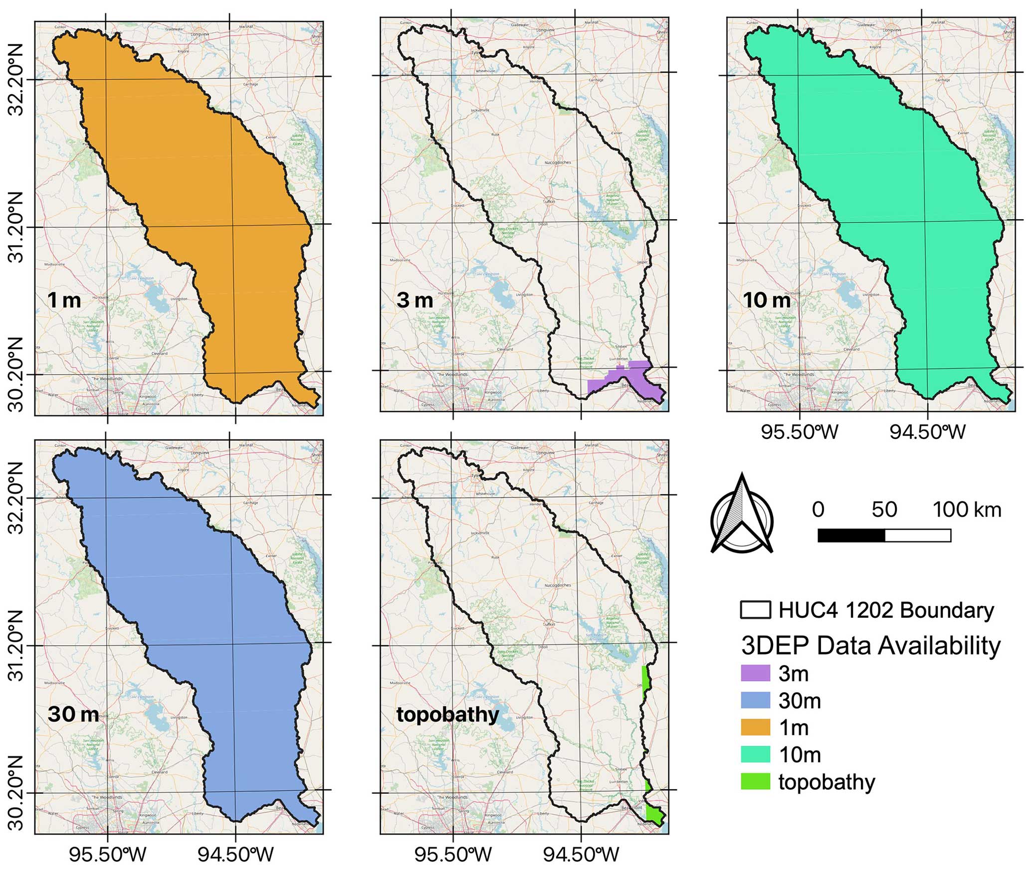
Figure 2 This figure illustrates the source digital elevation model (DEM) available within the 3D Elevation Program (3DEP) for the study area. High-resolution 1 m information is available for the entire study area, meaning it was used as the source resolution for resampling to the resolutions used for Height Above Nearest Drainage (HAND) computation, including 3, 5, 10, 15, and 20 m. See Sect. 2.5 for more information with regard to the study area. © OpenStreetMap contributors 2023. Distributed under the Open Data Commons Open Database License (ODbL) v1.0.

2.5 Study area

The site selection process considered several factors. The location of the site was limited by the availability of validation data (discussed in Sect. 2.6), as well as the availability of 1 m 3DEP information (USGS, 2022a, 2021b). Additionally, the location of the site was influenced by OWP's plan to release FIM services in stages as a function of the percentage of the population served. The first release will serve 10 % of the US population and cover portions of eastern Texas (TX), as well as the Mid-Atlantic states. On the other hand, the size of the evaluation site was constrained by the computational burdens of producing the FIM hydrofabric at multiple resolutions.

With these criteria in mind, we selected the Neches River sub-region as the study area for this experiment. The HUC-4 (1202) sub-region comprises seven HUC-8 sub-basins, ranging continuously from 12020001 to 12020007. Located in southeastern TX near the Louisiana border, the site stretches from Tyler to Beaumont and includes the towns of Nacogdoches and Lufkin, as depicted in Fig. 3. Numerous braided streams and 15 reservoirs, including one of the largest ones, the Sam Rayburn Reservoir, populate the study area. Figure 4 depicts the spatial distribution of LULCs as defined in the 2019 NLCD but grouped to the top tier of categories for visibility and interpretability. The study area features a low slope, with low-lying areas mostly comprising four LULCs: evergreen forests (31.1 %), pasture or hay (17.2 %), woody wetlands (16.7 %), and mixed forests (11.4 %). The developed LULCs together account for only 7.3 % of the site's area. In summary, the study area has low terrain slope and minimal anthropogenic influence.

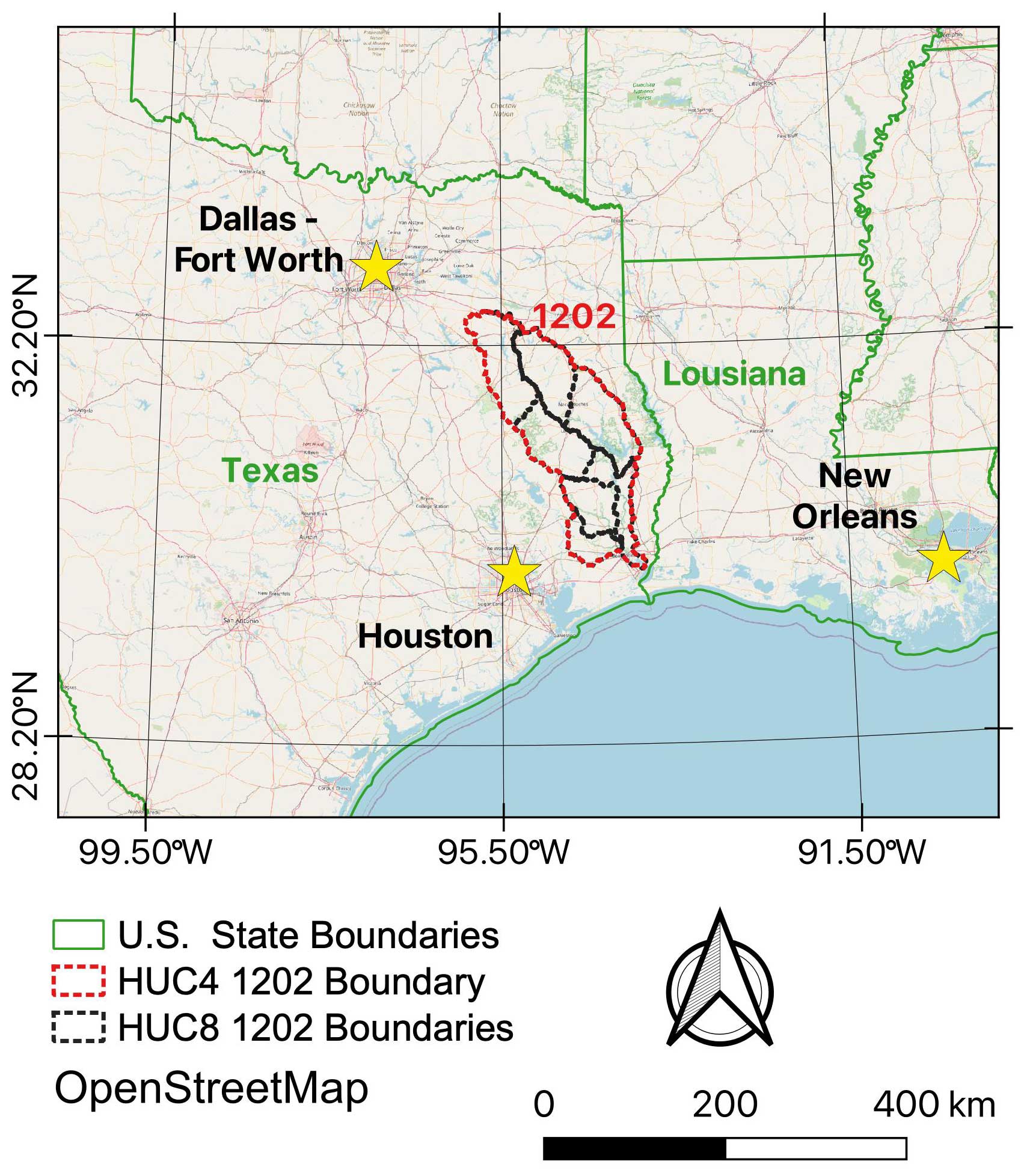
Figure 3 Overview of study area nestled in southeastern Texas (TX) near the Louisiana border. Known as the Neches River sub-region or HUC-4 1202, the site is composed of seven sub-basins or hydrologic unit code (HUC) 8s. © OpenStreetMap contributors 2023. Distributed under the Open Data Commons Open Database License (ODbL) v1.0.

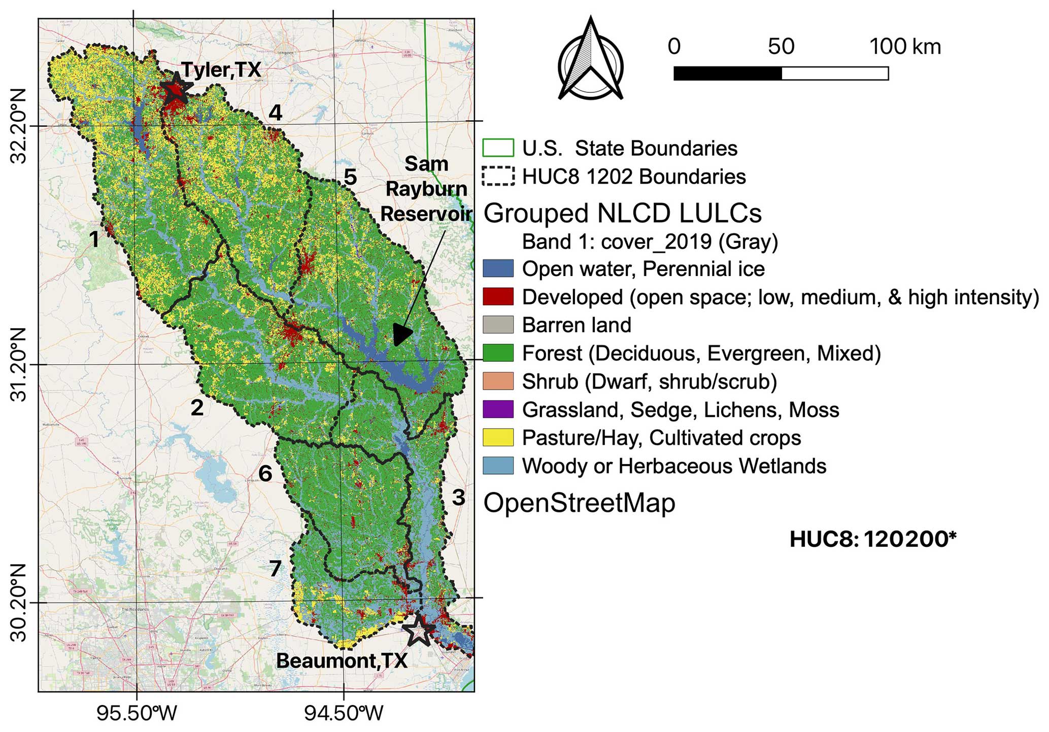
Figure 4 A detailed view showing the spatial distribution of the 2019 National Land Cover Database (NLCD) land use and land covers (LULCs) grouped to the top-tier categories for visibility and interpretability. About three-quarters of the site is made up of just four land covers, including evergreen forest (31.1 %), pasture or hay (17.2 %), woody wetlands (16.7 %), and mixed forests (11.4 %). Only about 7.2 % of the site is considered to be developed. © OpenStreetMap contributors 2023. Distributed under the Open Data Commons Open Database License (ODbL) v1.0.

2.6 Evaluation

We chose the BLE FIM extents for evaluation, which are HEC-RAS-1D-based models provided by InFRM and the Federal Emergency Management Agency (FEMA) (FEMA, 2016, 2021a, b; Strategic Alliance for Risk Reduction II, 2019a, b, c, d, e, f, g). FEMA's Region 6 publishes these FIMs, which are available at both 1 % (100-year) and 0.2 % (500-year) flow magnitudes, and they also include cross-sectional information with the associated flows for each level. Despite being a modeled dataset, HEC-RAS appears frequently in the literature for comparison purposes as it is an engineering-scale model (Cook and Merwade, 2009; Rajib et al., 2016; Zheng et al., 2018a; Afshari et al., 2018; Wing et al., 2017; Criss and Nelson, 2022; Follum et al., 2017). We chose to intersect the cross-sections with NWM flow paths to remove errors and uncertainties associated with hydrological and meteorological inputs used to produce streamflows within the NWM (Aristizabal et al., 2023c). This process enabled us to associate BLE-derived 100- and 500-year streamflow magnitudes with NWM forecasting points. If multiple intersections occurred per NWM stream reach, we took the median flow value. Even though this process may lead to conflation errors, we believe it allows for a better comparison with BLE FIM extents by removing any errors introduced from variances in other hydrological processes outside of inundation (Aristizabal et al., 2023c). For more detailed information on this technique and its application, see Sect. 2.7 in Aristizabal et al. (2023c). It is crucial to emphasize that the BLE benchmark FIMs utilize DEMs derived from high-quality lidar data, with a spatial resolution of approximately 1 m, for conducting hydraulic analyses and creating floodplain maps throughout our entire selected study region (Strategic Alliance for Risk Reduction II, 2019a, b, c, d, e, f, g). The benchmark's dependence on lidar-derived DEMs at 1 m resolutions enables the answering of our central question pertaining to the effect of DEM source and resolution on HAND-based FIM skill. We would like to acknowledge here that producing HAND with 1 m information to match that of the BLE is computationally very expensive, leading to substantial increases in central processing unit (CPU) time and memory usage, which we discuss in Sects. 3 and 4.

In order to quantify agreement with the BLE FIM extents, we elected to apply binary contingency statistics. The primary metrics calculated within a contingency table include true positives (TPs), false positives (FPs), false negatives (FNs), and true negatives (TNs). We again note that the positive condition is considered to be inundated, while the negative condition is considered to not be inundated. In order to summarize the contingency table into secondary metrics, we employed the commonly used metrics within flood modeling, including critical success index (CSI), true-positive rate (TPR), and false-alarm rate (FAR), shown in Eqs. (1)–(3), respectively (Gerapetritis and Pelissier, 2004; Schaefer, 1990).

$$\begin{array}{}\text{(1)}& {\displaystyle }& {\displaystyle }\mathrm{CSI}={\displaystyle \frac{\mathrm{TP}}{\mathrm{TP}+\mathrm{FP}+\mathrm{TN}}}\text{(2)}& {\displaystyle }& {\displaystyle }\mathrm{TPR}={\displaystyle \frac{\mathrm{TP}}{\mathrm{TP}+\mathrm{FN}}}\text{(3)}& {\displaystyle }& {\displaystyle }\mathrm{FAR}={\displaystyle \frac{\mathrm{FP}}{\mathrm{TP}+\mathrm{FP}}}\end{array}$$

TPR, also known as sensitivity, recall, and probability of detection or hit rate, was used to describe a model's ability to detect flooding as it represents performance in regions that are considered to be flooded within the benchmark. It is formally described as the proportion of inundated pixels that are accurately detected as flooded. FAR, also known as false-discovery rate, the inverse of precision, or the inverse of positive predictive value, conveys the opposite since it is used to represent over-prediction. This is formally described as the proportion of pixels incorrectly predicted to be flooded with respect to the total number of pixels predicted to be flooded. Work by Gerapetritis and Pelissier (2004) illustrated how these two metrics, TPR and FAR, are mathematically related to CSI where correctly predicted, non-inundated regions (TNs) are not considered. This leads to CSI being considered to be inequitable or exhibiting frequency dependency, which could limit its use in comparing predicted datasets in scenarios with varying frequencies (Gerapetritis and Pelissier, 2004; Schaefer, 1990).

While these three widely adopted metrics are considered to be highly interpretable, we elected to include the Matthews correlation coefficient (MCC), shown in Eq. (4), which is considered to be more equitable when dealing with cases of extreme class imbalance (Chicco and Jurman, 2020; Chicco et al., 2021a, b; Boughorbel et al., 2017). However, it does value both conditions (inundated and not inundated) as having equal impact (Chicco and Jurman, 2020; Chicco et al., 2021a, b; Boughorbel et al., 2017).

$$\begin{array}{}\text{(4)}& \mathrm{MCC}={\displaystyle \frac{\mathrm{TP}\cdot \mathrm{TN}-\mathrm{FP}\cdot \mathrm{FN}}{\sqrt{(\mathrm{TP}+\mathrm{FP})(\mathrm{TP}+\mathrm{FN})(\mathrm{TN}+\mathrm{FP})(\mathrm{TN}+\mathrm{FN})}}}\end{array}$$

2.6.1 Analysis

Evaluations for this HUC-4 study region were conducted at the HUC-8 scale, which produces seven HUC-8 metric values across all five spatial resolutions evaluated, as well as over both flood magnitudes, yielding about 70 samples to analyze ($\mathrm{7}\cdot \mathrm{5}\cdot \mathrm{2}=\mathrm{70}$). Analysis at this large HUC scale tends to erode away valuable information that could be used if a finer grain unit of measurement were used instead. Under this justification, we opted to sub-sample agreement maps down to the NWM catchment scale and recompute each of the four metrics for each catchment. There are 5786 NWM catchments available for this study area, which generates 405 020 effective samples to analyze ($\mathrm{70}\cdot \mathrm{5786}=\mathrm{405}\mathrm{020}$). This yielded a much finer grain spatial distribution of performance but also enabled the introduction of covariates and factors that can help explain some of the catchment-to-catchment variance in the metrics. Factors are categorical variables in our analysis and have a finite number of distinct categories. Covariates, on the other hand, are continuous variables that are assumed to have a linear relationship with the dependent variable. The term covariate serves the same function as the factors with the only distinction being that covariates are of continuous data types. We investigated the interaction of explanatory variables by multiplying all possible combinations to capture the variance in the dependent variable more comprehensively. The combination of covariates and factors was carried out by including interaction terms in the regression model. Interaction terms are created by multiplying a covariate and a factor or two factors, which allows us to investigate whether the effect of one variable depends on the level of the other variable. Many of these covariates and factors stemmed from NWM catchments or flow paths themselves, including channel slope, catchment area, stream order, and reservoir.

The term reservoir is used here with respect to catchments that intersect with NWM reservoirs. While NWM reservoirs are masked out for evaluation and are also not modeled within OWP FIM, the BLE FIM extents do model reservoir inundation. This creates regions of BLE inundation that extend beyond NWM reservoir definitions, thus leading to FNs. NWM catchments that intersect with NWM reservoirs are denoted as reservoir catchments and used as a factor to help account for the performance within these regions. This is better illustrated in Fig. 5.

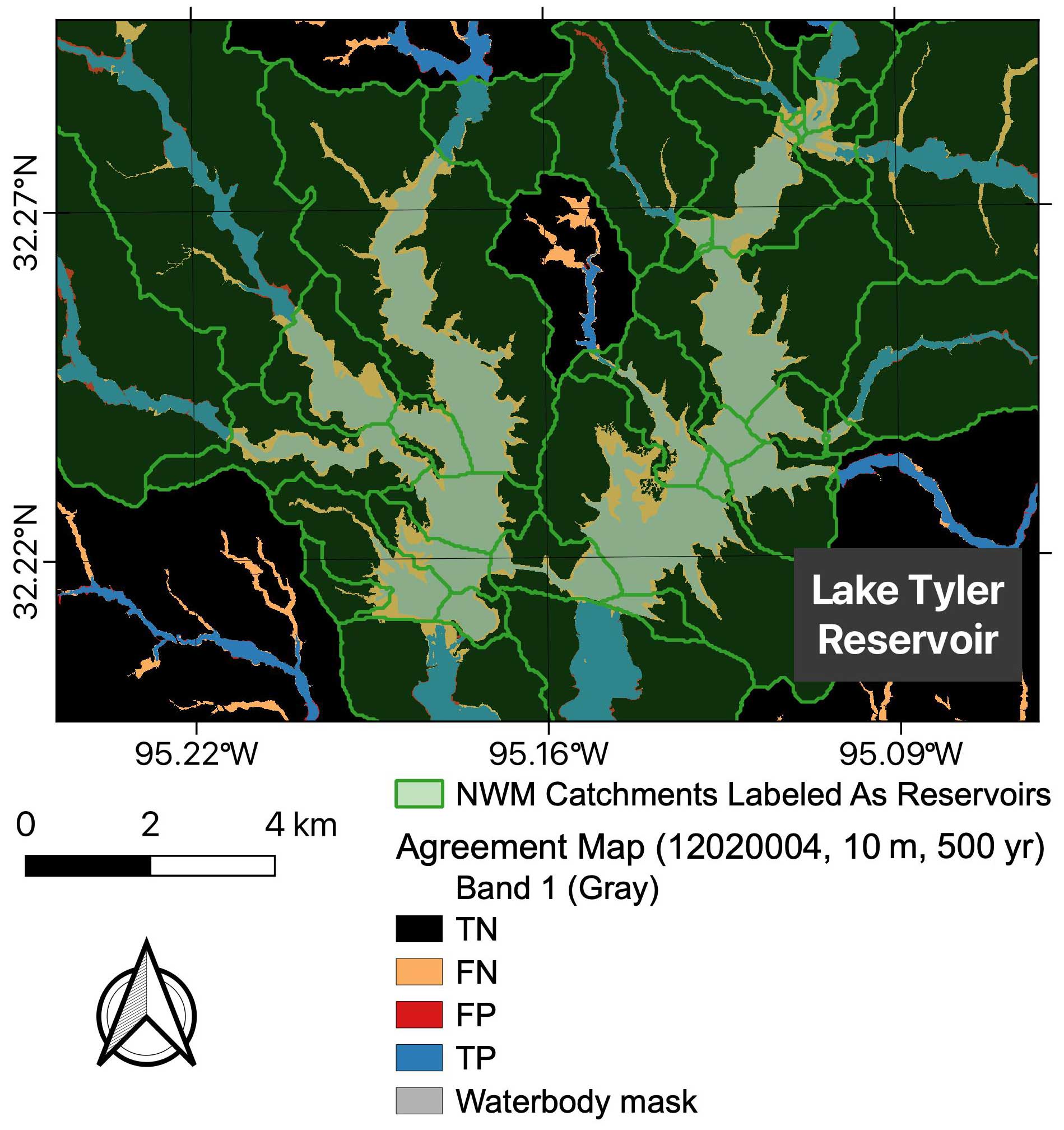
Figure 5 Figure shows Lake Tyler reservoir within hydrologic unit code (HUC)-8 12020004 of the study area. Background represents an agreement map between the Office of Water Prediction (OWP) flood inundation map (FIM) and the Base Level Engineering (BLE) FIM at a 10 m spatial resolution for the 500-year (yr) magnitude. Gray area shows masked-out National Water Model (NWM) reservoirs since these are not being modeled within OWP FIM. The NWM catchments shaded in green represent catchments associated with this NWM reservoir as they are shown to spatially intersect. These reservoir catchments were used in analysis to quantify the catchment variance in performance, partly due to not accounting for reservoir inundation within BLE FIM.

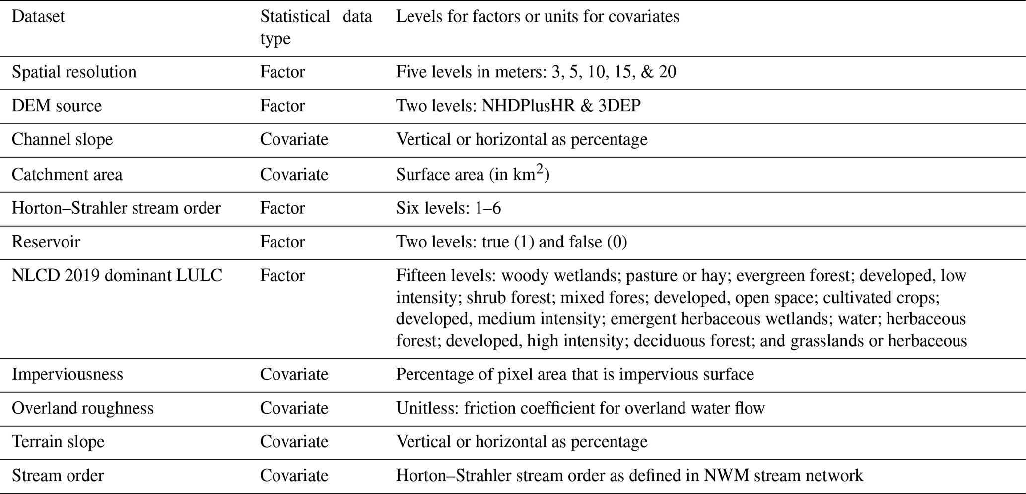
In addition to catchment-level attributes within the NWM hydrofabric, we collected a variety of datasets associated with hydrological processes, including NLCD LULC, imperviousness, overland roughness, and terrain slope. These factors and covariates were obtained utilizing the HyRiver suite of tools described in Sect. 2.3. Overland roughness was determined by the NLCD LULCs and previous research-assigned coefficients for each category (Dewitz, 2021; Yang et al., 2018; Chow, 1959; Chegini et al., 2021; Multi-Resolution Land Characteristics Consortium, 2022; McCuen et al., 2005; Kalyanapu et al., 2009). In order to aggregate to the catchment scale, LULC was taken as the dominant category by catchment, while the covariates' imperviousness, overland roughness, and terrain slope were aggregated by taking the catchment-level mean value. This procedure created a total of 10 catchment-level covariates and factors summarized as spatial resolution, DEM source, channel slope, catchment area, stream order, reservoir, LULC, imperviousness, overland roughness, and terrain slope. These covariates and factors are collectively known as features, predictors, explanatory variables, or independent variables and were used to correlate to dependent, response, or outcome variables which include the four metrics of interest in this study. These are described in more detail in Table 2.

Table 2 Summary of catchment-level covariates and factors used for statistical analysis. Included are the dataset, its statistical data type for analysis (factor or covariate), its units if it is a covariate, and its levels if it is a factor.

Given the fact that we aggregated a variety of catchment-scale features for each associated catchment-scale metric, we used the regression analysis to help explain the magnitude and significance of the linear relationships between the explanatory variables and the four responses (metrics: MCC, CSI, TPR, and FAR) (Montgomery et al., 2021; Chatterjee and Simonoff, 2013; Merrill et al., 2017). We avoided including the metrics with the NHDPlusHR DEM in the regression analysis since it was already clear that using 3DEP DEMs led to significant skill improvements. To build our regression model, we opted to use forward model selection of all one-way and two-way interactions utilizing the Akaike information criterion (AIC) and terminating the model selection after a minimum is reached. Explanatory variables were feature scaled from 0 to 1 prior to fitting to better compare across explanatory variables – meaning this procedure added variables to the regression model for each metric first. Identifying the explanatory variable that reduced the Akaike information criterion (AIC) to its minimum, the procedure retained this variable within the model before proceeding to evaluate the remaining variables, provided that the newly added variable offered an improvement of at least 0.001 over the preceding model. This process helps build models with explanatory power while avoiding unnecessary complexity.

3 Results

Based on the observation of our results, we conducted an in-depth analysis of the effects of utilizing 3DEP DEMs first when compared to the legacy NHDPlusHR DEMs. After confirming the positive effect of using 3DEP information, we varied the spatial resolution of these DEMs and observed the impact on performance. To further investigate the effects of additional explanatory variables, we built a multiple linear regression model with forward model selection to help explain some of the catchment-to-catchment variance in the four metrics. Lastly, we decided to do an in-depth analysis of a few of these variables that we found to be of importance.

3.1 3DEP data

For the given study area, we decided to investigate the effect on HAND-based FIM extents by utilizing the 3DEP data instead of the legacy source DEMs from the NHDPlusHR. We conducted this comparison on an NWM catchment scale in order to have a sense of the distribution of the results across some spatial definition finer than the HUC scale. Additionally, this comparison was conducted by resampling the 3DEP 1 m data to a spatial resolution of 10 m to match that of the legacy DEM. Figure 6 details the results of this comparison in a scatterplot format. Each individual data point represents a sample of the metrics taken at the NWM catchment scale. The points are sampled across two axes, representing their performance with NHDPlusHR DEMs on the x axis and with 3DEP DEMs on the y axis. The 45° diagonal line represents a dividing line where the metric values for both DEMs are the same. Catchment samples symbolized in green represent enhanced FIM extents for that catchment for the given case, while samples symbolized in red signify poorer-quality extents. We also included descriptive statistics on each sub-figure representing the mean and standard deviation of the metric differences across DEMs (3DEP − NHDPlusHR), as well as the percentage of differences greater than or less than zero.

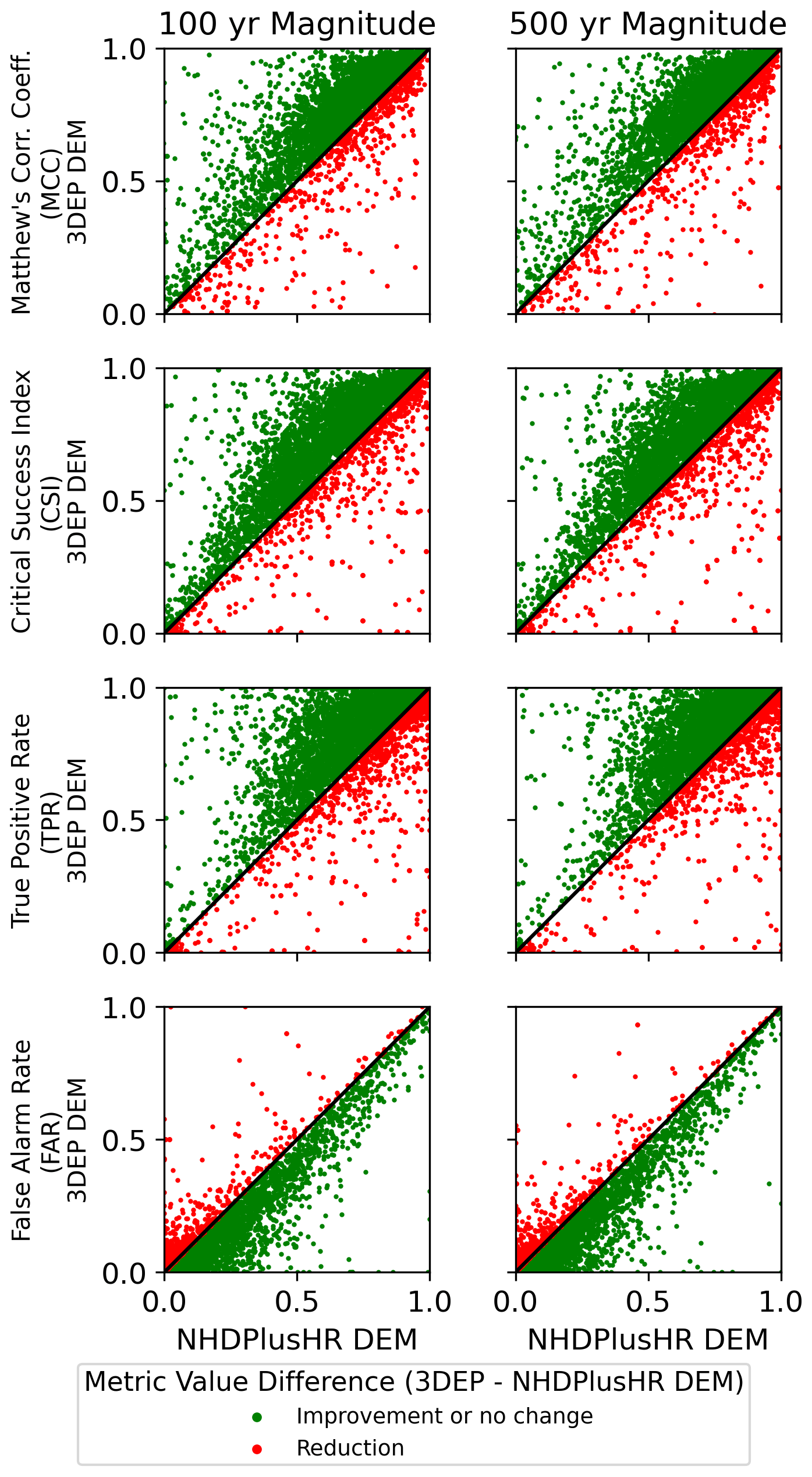
Figure 6 Figure shows catchment-scale metric values. The eight sub-figures are organized by magnitude (100 and 500 year) across the columns and for the four metrics across the rows. These values within each sub-figure are plotted on an axis representing Height Above Nearest Drainage (HAND)-based flood inundation maps (FIMs) generated from the National Hydrography Dataset Plus High Resolution (NHDPlusHR) digital elevation model (DEMs) (x axis) and the same FIMs generated from 3D Elevation Program (3DEP) DEMs resampled to the 10 m spatial resolution (y axis). The diagonal 45° line divides catchments that perform better with the legacy DEM (in red) and the catchments that perform better with the 3DEP DEM (in green). The majority of catchments perform better across all four metrics and both magnitudes with the higher-quality 3DEP information. Additional descriptive statistics quantifying the distribution of metric differences (3DEP–NHDPlusHR) are also presented, including the mean and standard deviation of the differences. We also included the percentage of samples whose difference is greater than or less than zero depending on the metric referenced.

Overall, the use of the higher-quality, more recently produced 3DEP DEMs generally enhances FIM extents across all the metrics and magnitudes examined. This is made evident by observing the high proportion of catchments represented in green and the high percentage of samples greater than zero for the first three metrics. The FAR is minimized, so a lower proportion of samples above zero is considered to be better. Overall, approximately four in every five catchments are considered to benefit from the use of 3DEP when compared to the use of NHDPlusHR. This approximate relationship holds true across metrics and event magnitudes for our given experimental design.

3.2 Regression analysis

After we established the effect of the new elevation data source on FIM extents, we elected to conduct regression analysis on the remaining explanatory variables of interest. As explained in the methods, we regressed the four metrics of interest independently and fit the model in a forward-selection fashion, utilizing AIC as a measure of model fit. Figure 7 represents the resulting models from that forward model selection in graphical form. The four subplots represent the results of the model fit to each metric or response variable. The y-axis labels represent explanatory variables, starting with the intercept followed by the remaining variables and their two-way interactions in the order of selection as per the AIC metric. By two-way interactions, we refer to the statistical interaction between pairs of explanatory variables, implying that the effect of one explanatory variable on the response variable may change depending on the value of another explanatory variable. The points on the graph represent the values of the coefficients, while the shape represents the level of significance from ≥0.05 (circle) to <0.05 (pentagon), <0.01 (triangle), and <0.001 (star). The green and red colors represent the nature of the effects as either positive (direct) or negative (indirect), respectively. Since AIC lacks interpretability, we elected to show the coefficient of determination or R² at each step of the forward-selection process. Additionally, Table 3 presents the results shown in Fig. 7 in a tabular format (Jann, 2005).

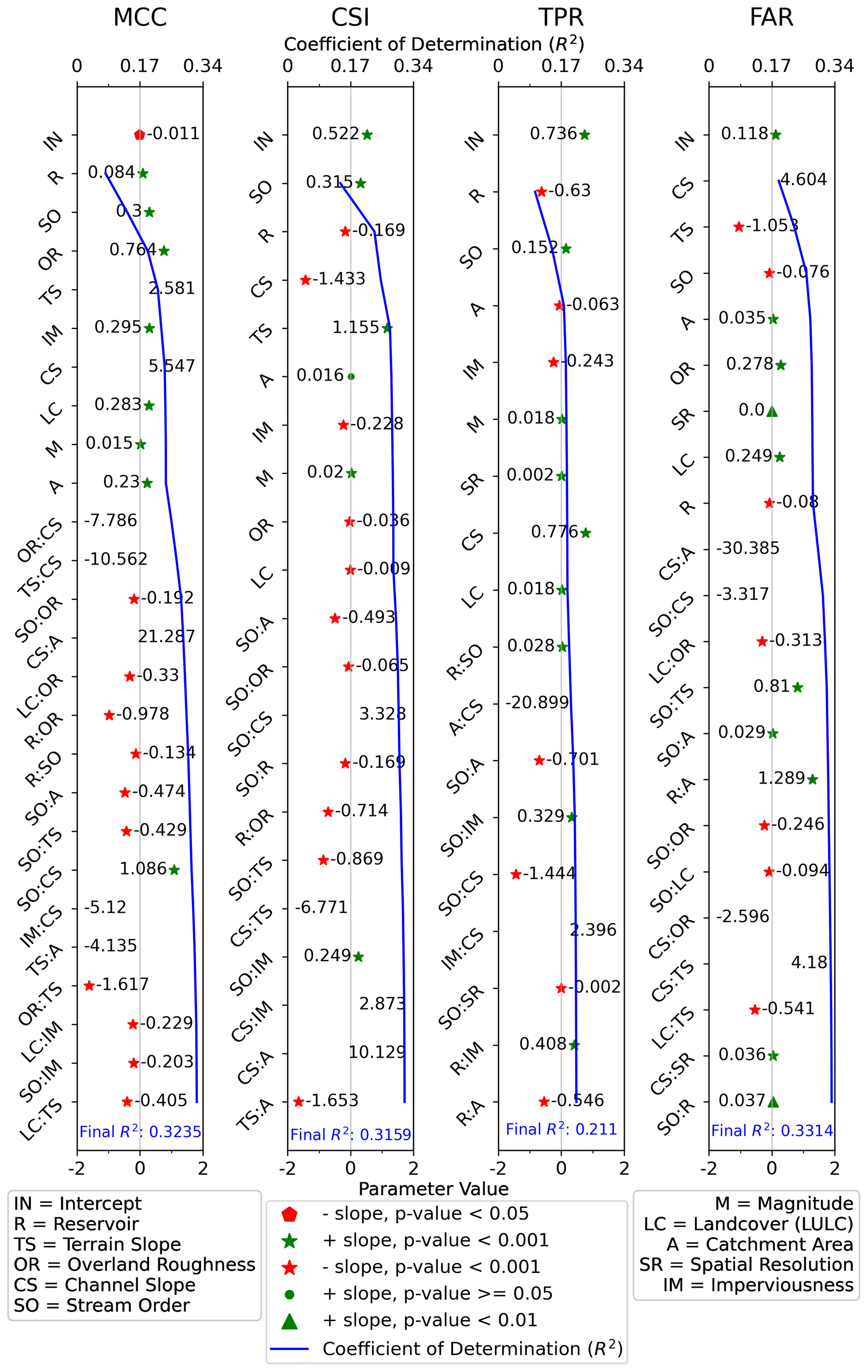
Figure 7 Figure illustrates the coefficients from multiple linear regression models fitted to four response variables independently. The points on the graph represent the values of the coefficients, while the shape represents the level of significance from ≥0.05 (circle) to <0.05 (pentagon), <0.01 (triangle), and <0.001 (star). The green and red colors represent the nature of the effects as either positive (direct) or negative (indirect), respectively. The models were built in a stepwise fashion using forward model selection and AIC as criteria for terminating the process. A total of 11 explanatory variables were considered for these models, as well as their two-way interactions. An intercept was also included by default. As the models built, we recorded the R² of each successive model and tracked as the complexity of the model increased. The final R² values for each final model are reported as well for each step of the forward selection.

Further examining Fig. 7, we can infer interesting pieces of information as regression analysis is a tool to synthesize data into something interpretable. The coefficients of determination or the R² values across the metrics vary from about 0.21 to 0.33. Translating this into other terms, one can say that about one-fifth to one-third of the catchment-to-catchment variance in the metrics can be explained by the 11 catchment-scale explanatory variables and their two-way interactions selected in this study. Additionally, observations from the figure illustrate the prevalence of certain explanatory variables near the beginning of the selection process that seem to explain a fair amount of the variation while also exhibiting strong effect sizes. Some of the variables of note include reservoir, stream order, terrain slope, channel slope, and LULC. These explanatory variables and their effect on catchment-level performance in FIM will be examined later on in Sect. 3.4.

Table 3 Regression analysis table showing coefficient values and their level of significance for each agreement metric. Coefficient values are based on feature-scaled explanatory variables in the range of 0 to 1. Variable definitions: intercept (IN), reservoir (RE), terrain slope (TS), overland roughness (OR), channel slope (CS), stream order (SO), magnitude (M), land cover (LC), catchment area (A), spatial resolution (SR), and imperviousness (IM).

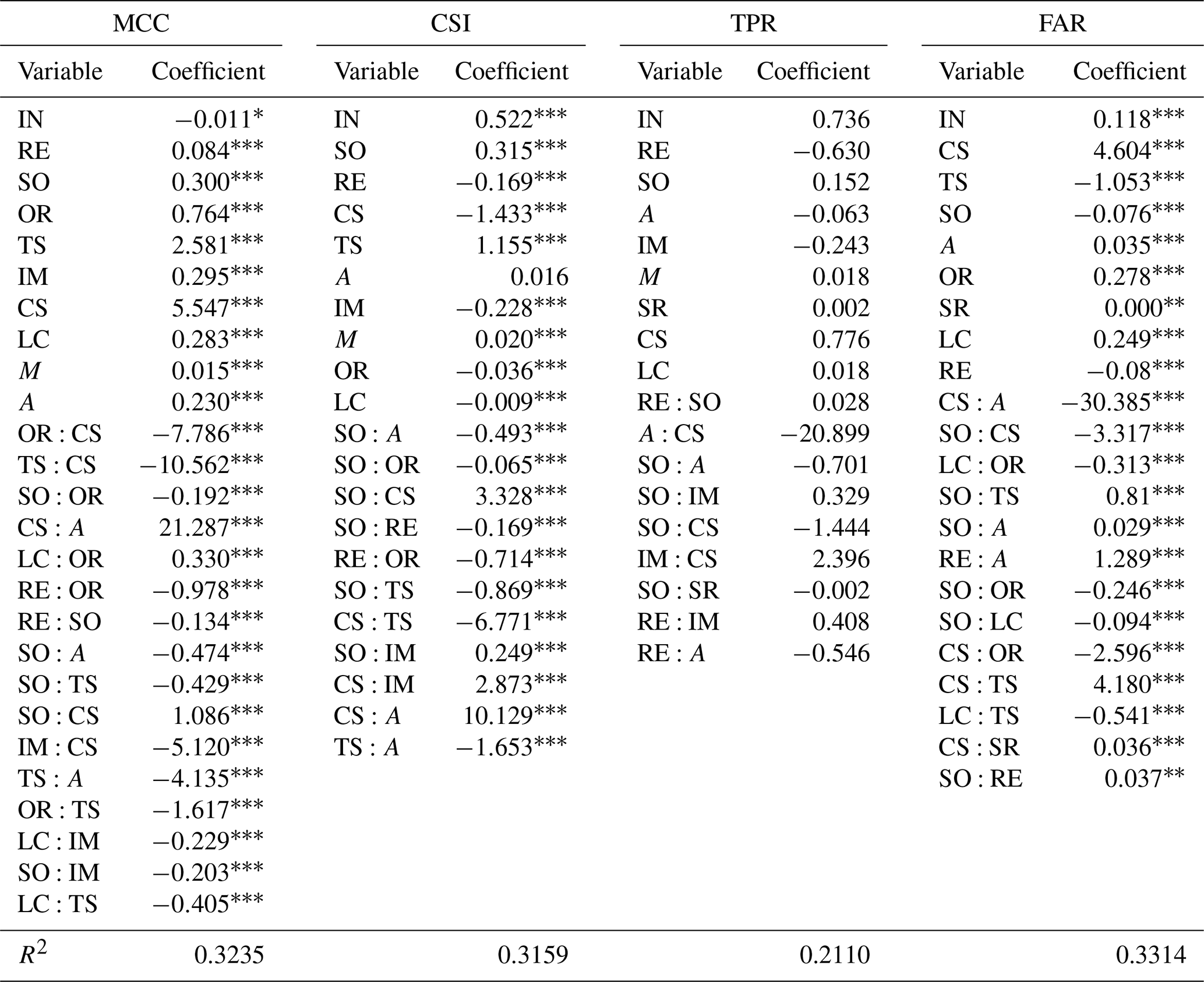
^* p≤0.05. ${}^{**}$ p≤0.01. ${}^{***}$ p≤0.001.

3.3 3DEP DEM spatial resolution

We investigated the effect of varying the spatial resolution of the 3DEP DEMs on the quality of FIMs produced from HAND. The 3DEP DEMs were varied at 3, 5, 10, 15, and 20 m prior to HAND computation.

Figure 8 examines the relationship of DEM spatial resolution at five levels for each of the four metrics selected. The relationships are illustrated as distributions of catchment-scale metric values for both event magnitudes (100 and 500 year). We computed the distributions as Gaussian kernel density estimations (KDEs), which is a non-parametric statistical technique that determines the probability distribution of a random variable (Virtanen et al., 2020; Scott, 2015; Silverman, 2018; Turlach et al., 1993; Bashtannyk and Hyndman, 2001). For each metric–magnitude distribution of catchment-scale metrics, the 75th, 50th, and 25th percentiles are calculated and displayed from top to bottom as dashed, solid, and dotted lines, respectively. Additionally, we fit two linear regression lines, one for each magnitude and for all four metrics, relating the linear effects of spatial resolution on metric values. The effect sizes, or the slopes of the regression lines, are displayed along with their respective p values. Low p values denote effect sizes that are unlikely to be equal to zero.

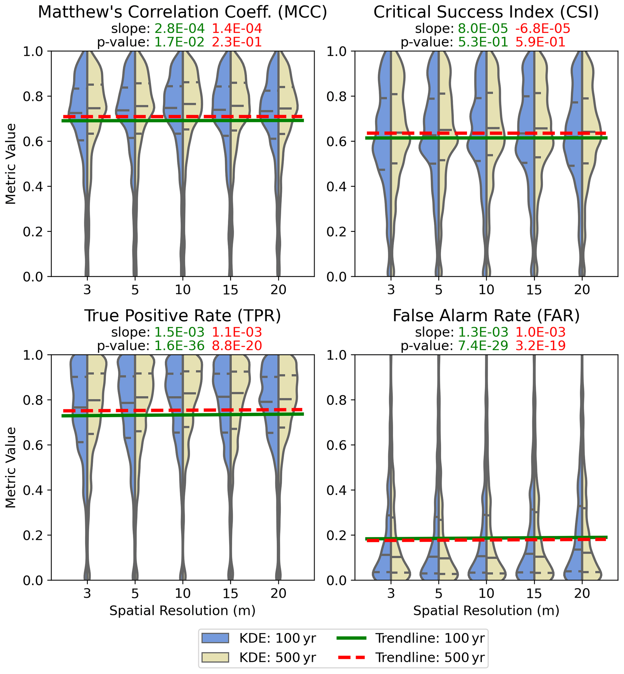
Figure 8 This figure illustrates the distribution of the four catchment-scale metrics as violin plots across every spatial resolution selected, including 3, 5, 10, 15, and 20 m. Each half of the violin represents a given magnitude of events (100 and 500 year). Linear trend lines are fit for each metric–magnitude combination, establishing linear relationships between spatial resolutions and metric values at the catchment scale.

Examination of Fig. 8 shows statistically significant yet marginal values in terms of effect sizes for the TPR and FAR metrics. For example, the effect size of the TPR and 100-year case is 0.0015, which represents a 0.0015 increase in the value of TPR for every meter increase in the magnitude of the resolution. Thus, for approximately 10 m, one would expect TPR to increase by 0.015. While coarser-resolution DEMs appear to improve the detection of inundation when compared to the BLE FIMs, they also appear to have an undesirable effect on FAR as its expected values increase as DEMs are coarsened. These competing effects on TPR and FAR seem to have a canceling effect on the overall performance metrics of MCC and CSI. Both MCC and CSI have statistically insignificant trend lines, which hints at little to no overall improvement in catchment-scale metrics of HAND-based FIM as a result of varying the spatial resolution of the input DEMs used to produce HAND.

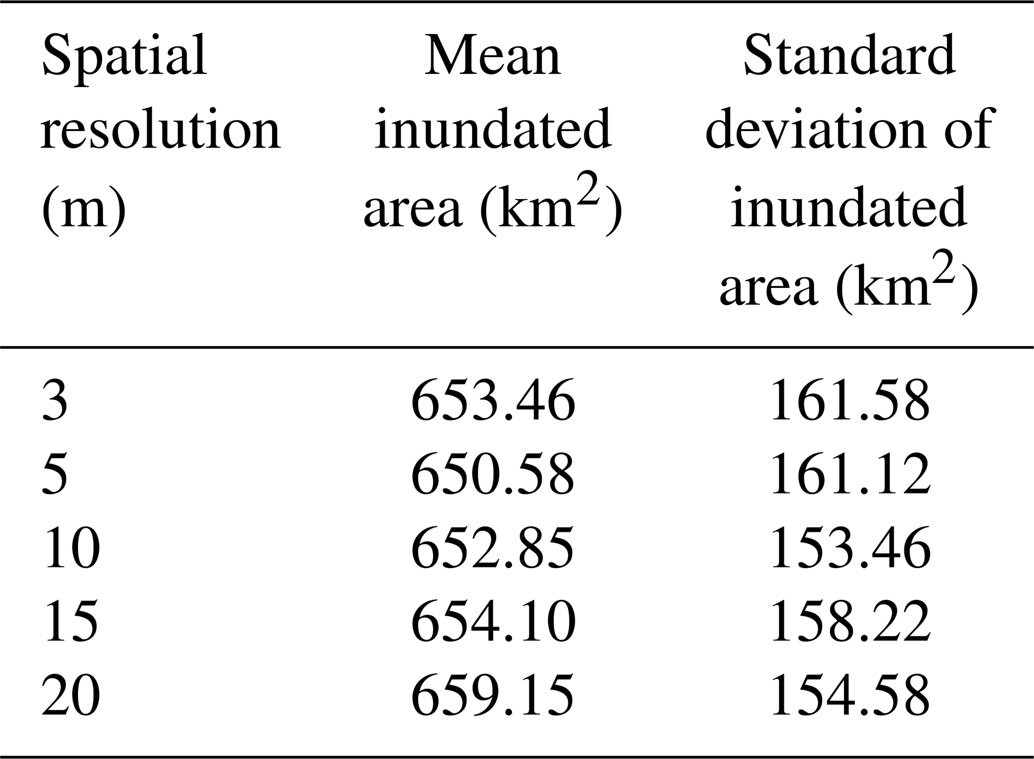
Furthermore, we analyzed the mean and standard deviations of the inundated areas for the five spatial resolutions selected. Table 4 shows the HUC-8 level mean and standard deviation of inundated areas (in km²) by spatial resolution and across magnitudes. Very little variation in the inundated areas was seen across the resolutions, which suggests that, while there was an increase in TPR and FAR with coarser DEMs, there is also little change in the inundated areas. This suggests that most of the trade-offs in resolution were related to trading type-I errors (FPs) in certain areas with type-II errors (FNs) in other areas, with little to no overall change in the inundated areas.

Table 4 Mean and standard deviations of inundated areas across hydrologic unit code (HUC) 8s and magnitudes (100 and 500 year) in square kilometers (km²) for each spatial resolution in meters (m).

A final observation related to the spatial resolution relates to its relatively low importance or the lack of interaction variables in the models built for the regression analysis in Sect. 3.2 and Fig. 7. This denotes that spatial resolution provided little to no effect when considering impactful variables such as LULC, imperviousness, stream order, or reservoir.

DEM resolution was found to have a significant effect on the computational demands of producing HAND. We aggregated the times to compute HAND at the seven DEM spatial resolutions and found a significant effect on CPU time, especially at finer resolutions. Figure 9 shows the change in log CPU times in seconds by HUC-8. A change of almost an entire order of magnitude in CPU time (in seconds) is observed when using DEMs of 3 m versus 20 m resolutions. The number of pixels for a given domain of squared pixels is known to have an inverse relationship with the square of spatial resolution (number of pixels∝squared resolution). Thus, reducing the spatial resolution from 10 to 1 m represents a 100-fold increase in the number of pixels for the fixed domain. It is important to note that all computational benchmarks were computed on an Amazon Web Services t3.2xlarge instance with eight processing units; 32 GB of memory; and a 2000 GB solid-state, elastic-block storage unit. The operating system was based on GNU/Linux with an Ubuntu 22.04 distribution on an x86 64-bit architecture. Despite having a minimal observed effect on skill, we found that higher resolutions tended to exhibit an excessive computational cost.

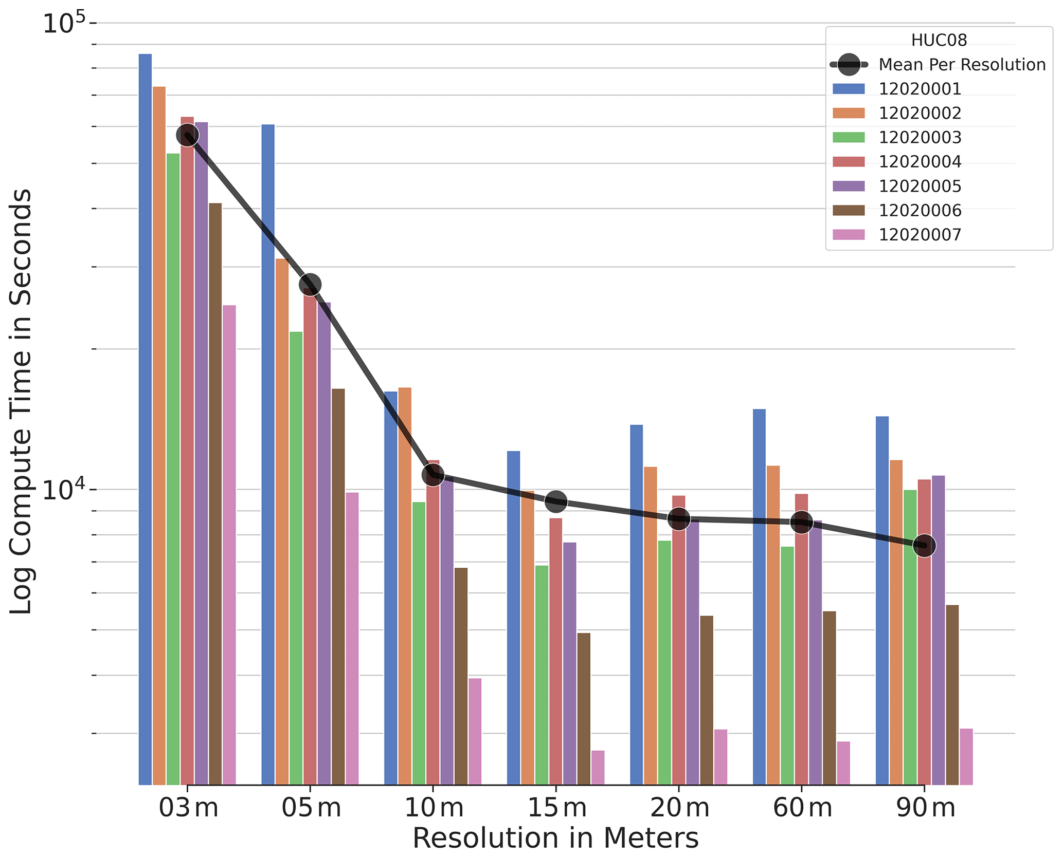
Figure 9 Total log central processing unit (CPU) time in seconds (s) across varying digital elevation map (DEM) spatial resolutions of 3, 5, 10, 15, 20, 60, and 90 m and listed by the seven hydrologic unit code (HUC) 8s in the study region. Resolution was found to have a significant effect on total CPU time for computing Height Above Nearest Drainage (HAND) as a reduction of nearly an entire order of magnitude in seconds was observed from changing the DEM resolution from 3 to 20 m. All computational benchmarks were computed on an Amazon Web Services t3.2xlarge instance with eight processing units; 32 GB of memory; and a 2000 GB solid-state, elastic-block storage unit. The operating system was based on GNU/Linux with an Ubuntu 22.04 distribution on an x86 64-bit architecture.

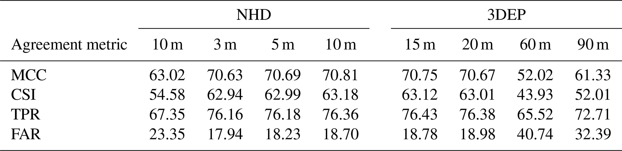
While this initial analysis demonstrates little influence of DEM spatial resolution on FIM extent quality, it also begged the following question: when might spatial resolution begin to exhibit some significant effect? In order to answer this question, the spatial resolutions of 60 and 90 m were selected and used to produce HAND and subsequent FIMs. These extents were again compared at the catchment scale for the entire study region for both 100- and 500-year flow magnitudes. Since 10 m is the current standard resolution for elevations within the NHDPlusHR and seamless 3DEP datasets, we illustrate the mean catchment-scale metrics across the entire study region for both flow magnitudes in Table 5. These results illustrate how spatial resolution does eventually exhibit a strong negative effect on FIM performance as the resolution is coarsened beyond the standard 10 m, which was specifically found to be around the medium resolutions between 20 and 60 m.

Table 5 Mean catchment-scale agreement metrics for the National Hydrography Dataset (NHD) (10 m resolution) and 3D Elevation Program (3DEP) (3, 5, 10, 15, 20, 60, and 90 m resolutions) digital elevation models (DEMs) across the entire study domain for both 100- and 500-year flow magnitudes. Values are presented as percentages (%) instead of native decimal values for readability.

3.4 Explanatory-variable focus

Since reservoirs and LULCs are valuable for forecasting operations, we elected to focus on those explanatory variables further within this analysis. Other variables, while important, were out of the scope of this paper but should be analyzed further in future studies.

3.4.1 Reservoirs

Given the relative importance of reservoirs in explaining catchment-to-catchment variance in many of the metrics, as shown in Fig. 7 and Sect. 3.2, we isolate this factor for further analysis here. Figure 10 shows the catchment-level distribution of the four metrics across spatial resolutions as violin plots built with KDEs. The halves of the violins are split across catchments that intersect with NWM reservoirs and those that do not. The trend lines, as well as their displayed slopes and p values, represent catchment-scale metric variance as a function of spatial resolution for each reservoir group.

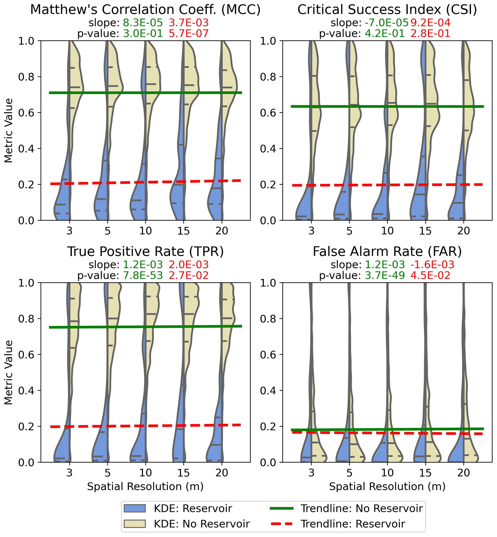
Figure 10 Catchment-scale variation illustrated as distributions modeled as kernel density estimations (KDEs). The distributions are grouped by metric and by spatial resolution. The halves of the violins are divided by the presence of a National Water Model (NWM) catchment that intersects (or does not intersect) an NWM reservoir. Significant differences are observed between catchments identified with and without reservoirs for all resolutions and metrics employed. Reservoirs are not currently modeled within the Office of Water Prediction (OWP) flood inundation map (FIM), while the Base Level Engineering (BLE) does account for reservoir-related inundation extents. While the NWM reservoirs are masked out for evaluation purposes, some of the BLE inundation extents reach beyond these boundaries, leading to a significant number of false negatives (FNs). The trend lines, as well as their corresponding slopes and p values, were constructed by regressing the two reservoir groups independently by spatial resolution. Little to no interaction between reservoir groups and spatial resolutions was observed.

Figure 10 primarily shows a large statistical difference in the catchment-scale variation of three metrics – MCC, CSI, and TPR – across the catchments that intersect with reservoirs and those that do not. Explaining this variation is simple as OWP FIM does not currently account for reservoir-related inundation, while the BLE does. While the NWM reservoirs are currently masked out for evaluation purposes, the BLE reservoir inundation extents go beyond these masked regions, thus contributing to FNs. Due to this fact, FAR illustrates very little performance difference across reservoir groups as FAR considers FPs and omits FNs (see Eq. 3). Another important trend to note from Fig. 9 is the relative lack of interaction between spatial resolution and the reservoir factor, as shown by the similarity in the slopes of trend lines across reservoir groups. This can be interpreted as spatial resolution having little effect across the reservoir groups, which can also be seen in Fig. 7, where the selection of a reservoir spatial resolution predictor was omitted. Until OWP FIM accounts for reservoir flooding or until some higher-order masking technique is applied, the presences of reservoir-related catchments will continue to contribute to a high variance in catchment-scale metrics.

3.4.2 Land use and land cover

We analyzed catchment-scale metrics by taking the dominant land cover per catchment (mode). While the linear analysis in Sect. 3.2 grouped the NLCD categories into two groups depending on their degree of anthropogenic influence, we decided to un-group the categories for Fig. 11. In this figure, we illustrate the distribution of the four catchment-scale metrics in box plots, which are grouped by both NLCD LULC and event magnitude. This chart does not appear to have a clear trend until further inspection leads one to see a pattern pertaining to the catchment-scale agreement and the nature of the LULCs. To reveal this trend, we decided to group LULC categories according to their relative level of anthropogenic influence.

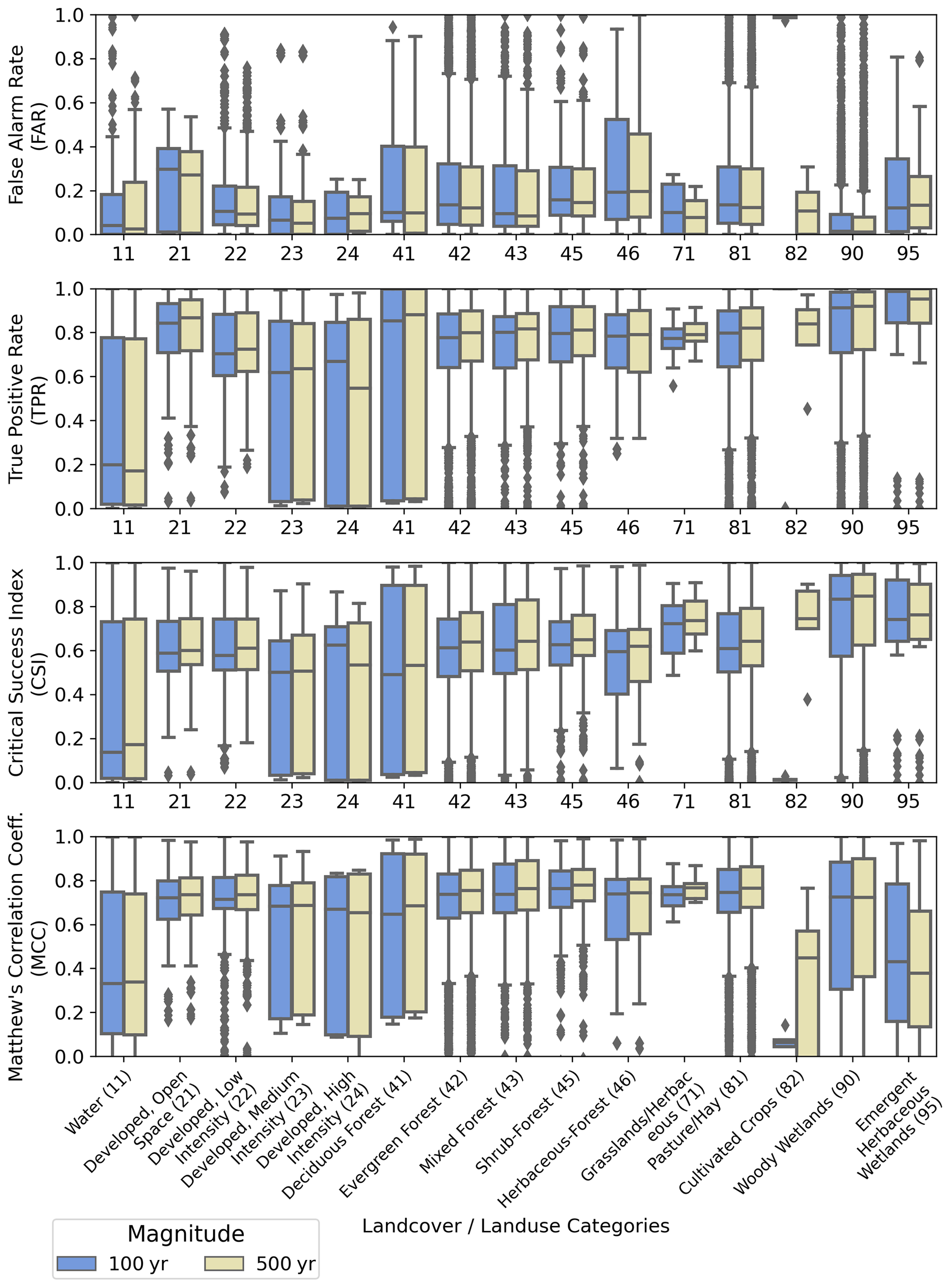
Figure 11 The distributions of four catchment-scale agreement metrics are shown as box plots and grouped by the dominant National Land Cover Database (NLCD) land use and land cover (LULC) per catchment, as well as the event magnitude.

In grouping the LULCs by two categories of “more” and “less” anthropogenic influence, we are able to see a clearer trend as to how LULC affects catchment-scale agreement. The LULCs grouped into the more category include the developed categories (open space, low intensity, medium intensity, and high intensity) and the cultivated-crops category, which, depending on the cropping system, can have significant hydrological implications. The remaining LULCs within the study area were placed in the less category. Figure 12 shows the distribution of catchment-scale metrics sorted by grouped LULC and event magnitude. We fit a multiple linear regression model for each metric using the grouped LULC and magnitude, as well as their interactions, as factors. The resulting formulas for this linear modeling are shown above each figure with the parameter values and their relative level of significance. Since only p values greater than 0.05 and less than 0.001 were encountered, we denoted those with no asterisk and three asterisks, respectively. Additionally, we plot the trend lines resulting from another regression that associates the metric values with the LULC grouping, and we do this for each event magnitude independently. Illustrating this regression demonstrates these relationships in a qualitative manner, highlighting the lack of interaction of event magnitude and grouped LULC.

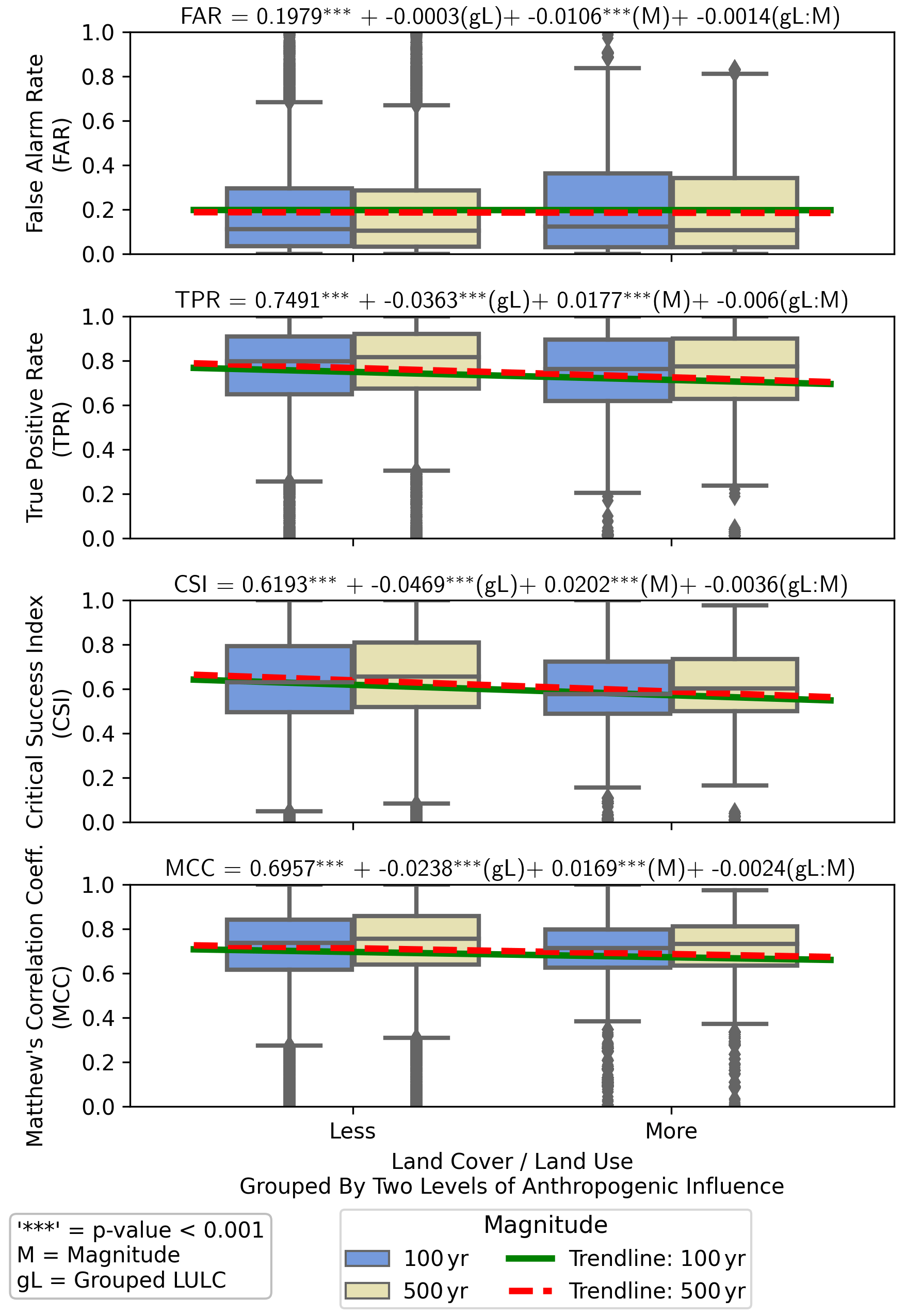
Figure 12 Distribution of catchment-scale agreement across four metrics illustrated as box plots and grouped by the level of anthropogenic influence in the National Land Cover Database (NLCD) land use and land covers (LULCs) and the two event magnitudes. The results of a linear model that regresses the catchment-scale metrics according to grouped LULC, magnitude, and their interaction are shown. The coefficients for the model are labeled with their p values by no asterisk and three asterisks for the p values greater than 0.05 and less than 0.001, respectively. Additionally, the trend lines resulting in a regression with catchment-scale metrics in grouped LULC are shown per event magnitude. It is important to note that LULC was found not to interact with spatial resolution within our regression analysis, meaning that various LULCs perform similarly across varying spatial resolutions.

Judging from Figs. 11 and 12, there is a clear indication that LULC has a significant influence over catchment-scale agreement. Grouped LULCs in Fig. 12 show the importance of anthropogenic influence in explaining catchment-scale variation in metric values, with a negative relationship being observed for having more relative anthropogenic influence. We found that LULC affected all the metrics except for FAR, where over-prediction was found not to be as affected by the anthropogenic influence. Under-prediction does appear to be prevalent in regions of anthropogenic influence, which could be explained by a variety of factors, including DEM inconsistencies or adverse effects on hydro-conditioning in areas with rapidly varying or uncertain elevations. It does appear that anthropogenic influence also contributes to more variation within the more case than in the less case, which could be a result of noise that is inherited from elevation inputs. While the magnitude per se is a significant factor in explaining catchment-scale agreement, it does not interact with grouped LULCs, meaning anthropogenic influence seems to have a similar effect across event magnitudes. Another interesting observation related to LULC is that the grouped LULCs do not seem to interact with spatial resolution. Thus, for this study area, higher resolutions did not provide an improvement in metrics for regions with more anthropogenic influence. We leave further analysis of the effect of LULCs and the anthropogenic influence on catchment-scale agreement to future work.

4 Discussion

Our results and analysis demonstrated several key methods that can improve the agreement of continental-scale FIMs using HAND when compared to engineering-scale FIM models. The inclusion of higher-quality terrain information from 3DEP was able to significantly improve the quality of continental-scale HAND-based FIMs. This finding is consistent with previous studies that have come to similar conclusions (Li et al., 2022; Zheng et al., 2018a; Garousi-Nejad et al., 2019; Speckhann et al., 2018) while also meeting the goal of the 3DEP objectives set out in justifying the collection effort (Dewberry, 2011; Snyder et al., 2013; Sugarbaker et al., 2014). As the program approaches continental-scale availability, 3DEP data can be justified for direct use in HAND computation for the entire US, leading to enhanced FIM and forecast quality.

However, varying the spatial resolution of the 3DEP DEMs from their native 1 m was found to have little effect on the quality of HAND-based FIMs, at least within 20 m resolution. Additional analysis extending comparisons of HAND-based FIMs at coarser resolutions, 60 and 90 m, revealed a significant degradation of performance at these scales. Previous studies examining this (Li et al., 2022; Zheng et al., 2018a; Garousi-Nejad et al., 2019; Speckhann et al., 2018) have varied in their experimental design and modeling assumptions. The modeling assumptions in those studies were different to those used in our HAND methods as we employ different datasets and hydro-conditioning procedures and compute HAND at finer scales (Aristizabal et al., 2023c). The experimental design of some previous studies (Zheng et al., 2018a; Garousi-Nejad et al., 2019) looked at high-resolution terrain data but did not explicitly isolate that factor for analysis purposes. Additionally, previous studies failed to denote a consistent relationship with spatial resolution and FIM performance (Li et al., 2022; Speckhann et al., 2018). While the mechanisms of this relationship have not been thoroughly explored with HAND, others have found that spatial resolution may have a spurious relationship with FIM performance due to inherent uncertainties related to this problem (Savage et al., 2016). Future research can expand the analysis of spatial resolution's effect on FIM quality to more study sites across broader domains of interest. Future research can also explore the effect spatial resolution may have on the quality of FIM depths as they likely behave somewhat independently to an extent. Additionally, we would like to motivate alternative benchmark datasets that could further our understanding of how DEM source and resolution affect the quality of HAND-based FIMs (Afshari et al., 2018). Utilizing 2D hydraulic models along with high-resolution and high-quality DEMs could furnish additional insights into this relationship as higher-order physics would produce varying extents compared to that of our 1D HEC-RAS benchmark (Afshari et al., 2018).

Further analysis sought to explain some of the catchment-level variation in the four agreement metrics with the aim of indicating where future progress can be made in extending FIM quality for continental-scale applications. As a result of the regression analysis, one-fifth to one-third of the catchment-scale variation of the agreement metric values was explained by building linear models with 11 explanatory variables and their two-way interactions. These models, while used for analysis purposes in this study, can have predictive performance, which could have calibration applications. Previous works have used a variety of methods to help calibrate Manning's n or bathymetry (Zheng et al., 2018b; Johnson et al., 2019; Jian et al., 2017; Neal et al., 2021; Liu et al., 2019). Due to the complex and interconnected nature of the source hydrography, hydro-conditioning operations, reach-averaged channel geometry, and Manning's n, any sort of calibration for SRCs would involve using the same sets of methods and datasets used to produce our version of HAND-based FIM.

Some of the explanatory variables were explored in further detail to provide insights into possible future skill improvements for OWP HAND-based FIM. Reservoirs were found to be one of the leading independent variables in explaining catchment-scale variation in three of the four metrics, mostly driven by under-prediction or FNs. These errors are caused by not accounting for reservoir inundation within OWP HAND FIM. Several methods exist for accounting for reservoir inundation, which could leverage volume computations with the NWM (Gochis et al., 2021; Chen et al., 2018; Shin et al., 2019). It is important to note here that, while reservoirs explained a significant amount of variation in the metrics, this does not mean that accounting for reservoir inundation properly would lead to a significant increase in agreement. Agreement will only change in response to the quality of the new method employed, as well as the prevalence of reservoir inundation in a given region. Another variable of interest further analyzed included the effect of LULC on agreement metrics. We found that HAND FIMs did not perform as well in catchments that are labeled as developed or cultivated crops. Regions of high anthropogenic influence negatively influence the performance of inundation models by adding extra complexity to the terrain information and the physics employed. Furthering the performance in these regions could benefit from the use of hyper-resolution models that better account for urban water features (Grimley et al., 2017; Smith et al., 2020; Deo et al., 2018; Gurung et al., 2018; Smith et al., 2021; Leandro et al., 2016; Chegini et al., 2021). Further exploring these and other independent variables could help inform future development directions to help improve the quality of continental-scale FIM techniques.

5 Conclusions

Floods are a significant source of natural disasters in the United States (US), leading to loss of property and lives. The National Oceanic and Atmospheric Administration's Office of Water Prediction (OWP) has implemented the National Water Model (NWM) to help forecast streamflows at nearly 3 million locations across the continuous US, Hawaii, Puerto Rico, and portions of Alaska at hourly time steps and multiple forecast horizons. OWP has developed its own version of Height Above Nearest Drainage (HAND) that accounts for multiple fluvial sources of inundation instead of just that from the local, nearest flow path. The United States Geological Survey's 3D Elevation Program is rapidly approaching continental-scale availability of digital elevation maps (DEMs), so we evaluated its use at 10 m spatial resolution within the derivation of HAND and found significant increases in the quality of FIM performance. Additionally, we varied the resolution to include 3, 5, 15, and 20 m but did not find any significant trends on an overall basis, leading one to justify its use within these study regions. However, a significant degradation in FIM skill was observed at the coarser resolutions of 60 and 90 m. As one would expect, the computational time increased to compute HAND with the number of DEM cells considered, which goes up with the inverse of the DEM resolution squared. We determined that more studies are required in other regions to help explore the potential benefits of the use of higher-resolution DEMs along with HAND. A multiple linear regression model fitting 11 factors and covariates to the four agreement metrics, all at the catchment scale, revealed that about one-fifth to one-third of the variation can be explained by these explanatory variables.