Technical note: Analytical solution for well water response to Earth tides in leaky aquifers with storage and compressibility in the aquitard

In recent years, there has been a growing interest in utilizing the groundwater response to Earth tides as a means of estimating subsurface properties. However, existing analytical models have been insufficient in accurately capturing realistic physical conditions. This study presents a new analytical solution to calculate the groundwater response to Earth tide strains, including storage and compressibility of the aquitard, borehole storage, and skin effects. We investigate the effects of aquifer and aquitard parameters on the well water response to Earth tides at two dominant frequencies (O₁ and M₂) and compare our results with hydraulic parameters obtained from a pumping test. Inversion of the six hydro-geomechanical parameters from amplitude response and phase shift in both semi-diurnal and diurnal tides provides relevant information about aquifer transmissivity, storativity, well skin effect, aquitard hydraulic conductivity, and diffusivity. The new model is able to reproduce previously unexplained observations of the amplitude and frequency responses. We emphasize the usefulness in developing a relevant methodology to use the groundwater response to natural drivers in order to characterize hydrogeological systems.

1 Introduction

Aquifer properties play a vital role in managing groundwater resources, particularly amid increasing anthropogenic groundwater use and the impact of climate change. While pump testing can be costly, there exists a cost-effective alternative for assessing aquifer hydraulic properties – analysing the groundwater response to Earth tides or atmospheric tides (McMillan et al., 2019; Valois et al., 2023). Observations of variations in groundwater level due to tidal fluctuations date back to the works of Klönne (1880), Meinzer (1939), and Young (1913). However, it was only later that hydro-geomechanical models were employed to elucidate these variations (Bredehoeft, 1967; Hsieh et al., 1987; Roeloffs, 1996; Wang, 2000; Cutillo and Bredehoeft, 2011; Kitagawa et al., 2011; Lai et al., 2013; Wang et al., 2018). This progression in understanding offers a valuable opportunity to evaluate aquifer hydraulic properties through the response of groundwater to Earth tide strain fluctuations within the aquifer system.

Hsieh and Bredehoeft (1987) introduced the horizontal-flow model, focusing on confined conditions influenced by tidal strain within the aquifer. Conversely, Roeloffs (1996) and Wang (2000) explored interactions within vertical flow under tidal fluctuations. Wang et al. (2018) expanded on these studies by incorporating a flow from an upper aquitard, albeit assuming negligible storage within it. Later, Gao et al. (2020) extended these models to include borehole skin effects. A definition of the skin effect can be found in Wen et al. (2011). Thomas et al. (2023) developed an Earth-tide–groundwater (ET-GW) model incorporating storage and strain response in the aquitard. They applied their model to a specific site to evaluate transmissivity variations and validated it using pumping tests.

Numerous studies have investigated aquifer hydromechanical properties by analysing groundwater (GW) level variations induced by Earth tides, employing the models mentioned in the previous literature (Narasimhan et al., 1984; Merritt, 2004; Fuentes-Arreazola et al., 2018; Zhang et al., 2019a; Shen et al., 2020). Some studies focused also on the tidal response in fractured rock aquifers (Carr and Van Der Kamp, 1969; Bower, 1983; Burbey et al., 2012; Rahi and Halihan, 2013; Sedghi and Zhan, 2016). However, only a limited number of validations have been conducted, which involve comparing the results with robust hydraulic assessments, such as hydraulic conductivity derived from slug testing (Zhang et al., 2019b) or specific storage and transmissivity characterizations obtained through long-term pumping tests (Allègre et al., 2016; Valois et al., 2022). The current evaluations predominantly focus on purely confined conditions, leaving a gap in knowledge regarding tidally induced GW responses in aquifers under semi-confined conditions.

As far as the authors are aware, the publications by Sun et al. (2020), Valois et al. (2022), and Thomas et al. (2023) are the sole references addressing a comparison for a leaky aquifer. Sun et al. (2020) found significant discrepancies between transmissivities obtained from Earth tide fluctuations and those derived from slug or pump tests. However, it is worth noting that the comparison may be subject to discussion, as the authors employed a leaky aquifer model for analysing tidally induced fluctuations, whereas they used a confined aquifer model for conducting slug and pump tests. In the study conducted by Valois et al. (2022), the existing ET-GW models, as described earlier, were unable to reproduce a low ratio of semi-diurnal to diurnal amplitude with positive phase shifts in conjunction with pumping test transmissivity data. This discrepancy highlights the complexity and challenges in modelling tidally induced groundwater responses in leaky aquifers and the need for further investigation in this area.

We note that our previous attempts to model the observed substantial amplitude decrease from the diurnal tide (O₁) to the semi-diurnal tide (M₂) frequency, combined with phase shifts close to zero, proved unsuccessful when using Earth tide models found in the literature. None of the existing models could provide satisfactory results. The pursuit of an explanation led to the realization that analytical solutions with more realistic assumptions are required. For example, aquifers are widely recognized to be influenced by aquitards, which often consist of highly porous and compressible clay materials, contributing significant amounts of stored water to the aquifer (Moench, 1985). Moreover, these aquitards are also impacted by Earth tide strains (Bastias et al., 2022).

Our first objective is to develop an analytical solution considering storage and tidal strain in the aquitard. Unlike Thomas et al. (2023), our model incorporates borehole skin effects and allows for a fixed hydraulic head at the top of the aquitard, broadening its applicability to a broader range of hydrogeological conditions. The second motivation of our study is to develop a model that better fits the observed results by considering aquitard storage, as evident in the pumping tests. Third, we compare the results obtained from our new ET-GW model with those derived from a pumping test in leaky aquifers with storage in the aquitard. Fourth, since most publications have predominantly focused on assessing hydraulic properties using the semi-diurnal tide (M₂), our third motivation is to demonstrate the potential of using diurnal tides (O₁) in combination with the semi-diurnal ones (M₂ or N₂) to provide a more comprehensive characterization of aquifer and aquitard hydromechanical properties. Our new development offers the potential to enhance hydraulic and geomechanical subsurface characterization by employing a more realistic model for the groundwater response to natural forces.

2 Groundwater response to Earth tides in a leaky aquifer with aquitard storage and strain

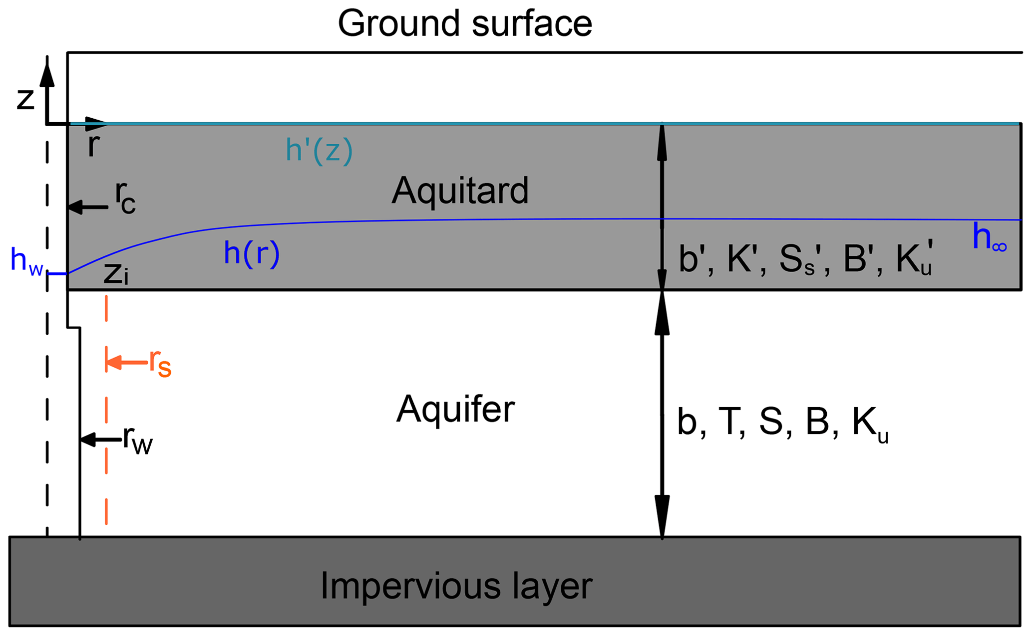
Hantush (1960) pioneered the modelling of aquitard storage by modifying the leaky aquifer theory to account for storage in the aquitard. In our study, we consider a semi-confined configuration (Fig. 1) where the target aquifer is overlain by an aquitard that allows for storage, strain, and vertical flux. Both layers are assumed to be slightly compressible, spatially homogenous, and infinite laterally and to have constant thickness. Building upon the work of Wang et al. (2018), our research incorporates Earth tide (ET) fluctuations into the leaky aquifer equations proposed by Moench (1985). Additionally, we incorporate the skin effect, as described by Gao et al. (2020). Two-dimensional cylindrical coordinates are used because of the radial symmetry caused by the well surrounded by hydrogeological material affected by tidal strain.

Groundwater flow and storage in an aquifer overlain by an aquitard can be described as (De Marsily, 1986):

$$\begin{array}{}\text{(1)}& {\displaystyle }T\left({\displaystyle \frac{{\partial }^{\mathrm{2}}h}{\partial r^{\mathrm{2}}}}+{\displaystyle \frac{\mathrm{1}}{r}}{\displaystyle \frac{\partial h}{\partial r}}\right)=S\left({\displaystyle \frac{\partial h}{\partial t}}-{\displaystyle \frac{B{K}_{\mathrm{u}}}{\mathit{\rho }g}}{\displaystyle \frac{\partial \mathit{\epsilon }}{\partial t}}\right)-K^{\prime }{\displaystyle \frac{\partial h^{\prime }}{\partial z}},\text{(2)}& {\displaystyle }\left({\displaystyle \frac{{\partial }^{\mathrm{2}}{h}^{\prime }}{\partial z^{\mathrm{2}}}}\right)={\displaystyle \frac{\mathrm{1}}{D^{\prime }}}\left({\displaystyle \frac{\partial h^{\prime }}{\partial t}}-{\displaystyle \frac{B^{\prime }{K}_{\mathrm{u}}^{\prime }}{\mathit{\rho }g}}{\displaystyle \frac{\partial \mathit{\epsilon }}{\partial t}}\right).\end{array}$$

Here, h (m) and h^′ (m) are the hydraulic heads in the aquifer and the aquitard respectively; $h_j^{\prime }$ (m) is the fixed hydraulic head at the top of the aquitard; r (m) is the radial distance from the studied well; T (m² s⁻¹) and S are the aquifer transmissivity and storativity; B, B^′, K_u (Pa), and $K_{\mathrm{u}}^{\prime }$ (Pa) are Skempton's coefficient and the undrained bulk modulus of the aquifer and aquitard; ρ (kg m⁻³) and g (m s⁻¹) are the water density and gravity constant; ε is the volumetric Earth tide strain; K^′ (m s⁻¹) is the aquitard hydraulic conductivity; $S_{\mathrm{s}}^{\prime }$ (m⁻¹) is the specific storage of the aquitard; and D^′ (m² s⁻¹) is aquitard hydraulic diffusivity ($K^{\prime }/S_{\mathrm{s}}^{\prime }$ ratio). Any natural regional groundwater flow is considered negligible.

Borehole drilling causes a zone of damage with a radius r_s (see Fig. 1) that is responsible for the skin effect (Van Everdingen, 1953). A negative skin can be caused by a greater hydraulic conductivity around the well because of the material damaged by the drilling, while a positive skin can be associated by porosity clogging caused by the drilling mud. This is reflected in the well's pressure head Δh_s. The skin factor (sk) can be defined as

$$\begin{array}{}\text{(3)}& \mathrm{sk}={\displaystyle \frac{\mathrm{\Delta }{h}_{\mathrm{s}}}{{\left(r\frac{\partial h}{\partial r}\right)}_{r=r_{\mathrm{w}}}}}.\end{array}$$

Following above assumptions, the boundary conditions are

$$\begin{array}{}\text{(4)}& {\displaystyle }h\left(r,t\right)=h_{\mathrm{\infty }}\left(t\right)\mathrm{at}r=\mathrm{\infty },\text{(5)}& {\displaystyle }{h}_{\mathrm{w}}\left(t\right)=h\left(r,t\right)-\mathrm{sk}\left(r{\displaystyle \frac{\partial h\left(r,t\right)}{\partial r}}\right)\mathrm{at}r=r_{\mathrm{w}},\text{(6)}& {\displaystyle }\mathrm{2}\mathit{\pi }{r}_{\mathrm{w}}T{\left({\displaystyle \frac{\partial h}{\partial r}}\right)}_{r=r_{\mathrm{w}}}=\mathit{\pi }{r}_{\mathrm{c}}^{\mathrm{2}}{\displaystyle \frac{\partial h_{\mathrm{w}}}{\partial t}},\text{(7)}& {\displaystyle }{h}^{\prime }=h\mathrm{at}z=z_{\mathrm{i}},\text{(8)}& {\displaystyle }{h}^{\prime }=h_j^{\prime }\mathrm{at}z=\mathrm{0}.\end{array}$$

Here, t is the time (s); r_w and r_c are the radius of the well-screened portion and the radius of well casing in which the water level fluctuates; z_i is the aquifer–aquitard interface elevation (see Fig. 1) and h_w is the hydraulic head at r_w.

Figure 1 Semi-confined system with a compressible aquitard with storage.

Following Hsieh et al. (1987) and Wang et al. (2018), complex numbers were used to facilitate harmonic model development, and the solution is obtained by first solving Eq. (2) in the aquitard and then deriving the head response in the aquifer far away from the well (h_∞), which is independent of the radial distance. h_∞ is the aquifer response to the tidal harmonic sources far from the well. Thus, h_∞ is the aquifer hydraulic head response without any disturbance from a well–aquifer system. Then, the well effect on the aquifer response is considered by using a flux condition at the well that accounts for wellbore storage. Since h^′, h, ε,h_w, and h_∞ are all periodic functions, they can be expressed as

$$\begin{array}{}\text{(9)}& {\displaystyle }\mathit{\epsilon }\left(t\right)={\mathit{\epsilon }}_{\mathrm{0}}{e}^{i\mathit{\omega }t},\text{(10)}& {\displaystyle }{h}_{\mathrm{\infty }}\left(t\right)=h_{\mathrm{\infty },\mathrm{0}}{e}^{i\mathit{\omega }t},\text{(11)}& {\displaystyle }{h}_{\mathrm{w}}\left(t\right)=h_{\mathrm{w},\mathrm{0}}{e}^{i\mathit{\omega }t},\text{(12)}& {\displaystyle }h(r,t)=h_{\mathrm{0}}\left(r\right)e^{i\mathit{\omega }t},\text{(13)}& {\displaystyle }{h}^{\prime }(z,t)=h_{\mathrm{0}}^{\prime }\left(z\right)e^{i\mathit{\omega }t}.\end{array}$$

Here, $i=\sqrt{-\mathrm{1}}$; ε₀ (−) is the ET strain amplitude and ω (s⁻¹) is the angular frequency. In this case, Eq. (2) becomes

$$\begin{array}{}\text{(14)}& \left({\displaystyle \frac{{\partial }^{\mathrm{2}}{h}_{\mathrm{0}}^{\prime }}{\partial z^{\mathrm{2}}}}\right)={\displaystyle \frac{\mathrm{1}}{D^{\prime }}}\left(i\mathit{\omega }{h}_{\mathrm{0}}^{\prime }-i\mathit{\omega }{\displaystyle \frac{B^{\prime }{K}_{\mathrm{u}}^{\prime }}{\mathit{\rho }g}}{\mathit{\epsilon }}_{\mathrm{0}}\right).\end{array}$$

According to Wang (2000) and Roeloffs (1996) and as detailed in Appendix A, the solution of Eq. (2) is

$$\begin{array}{}\text{(15)}& h_{\mathrm{0}}^{\prime }=A_{\mathrm{1}}{e}^{\frac{\left(\mathrm{1}+i\right)}{\mathit{\delta }}(z-z_{\mathrm{i}})}+A_{\mathrm{2}}{e}^{-\frac{\left(\mathrm{1}+i\right)}{\mathit{\delta }}(z-z_{\mathrm{i}})}+{\displaystyle \frac{B^{\prime }{K}_{\mathrm{u}}^{\prime }}{\mathit{\rho }g}}{\mathit{\epsilon }}_{\mathrm{0}},\end{array}$$

where $\mathit{\delta }={\left(\frac{\mathrm{2}{D}^{\prime }}{\mathit{\omega }}\right)}^{\mathrm{1}/\mathrm{2}}$. Thus, at the interface between the aquifer and the aquitard (z=z_i), we have pressure continuity as $h^{\prime }\left(z_{\mathrm{i}},t\right)=h_{\mathrm{0}}{e}^{i\mathit{\omega }t}=h\left(t\right)$ which leads to

$$\begin{array}{}\text{(16)}& {\left({\displaystyle \frac{\partial h^{\prime }}{\partial z}}\right)}_{z=z_{\mathrm{i}}}={\displaystyle \frac{\mathrm{1}+i}{\mathit{\delta }}}\left({\displaystyle \frac{h_{\mathrm{0}}-\frac{B^{\prime }{K}_{\mathrm{u}}^{\prime }}{\mathit{\rho }g}{\mathit{\epsilon }}_{\mathrm{0}}}{\tan h\left(\frac{\mathrm{1}+i}{\mathit{\delta }}{z}_{\mathrm{i}}\right)}}-{\displaystyle \frac{h_j^{\prime }-\frac{B^{\prime }{K}_{\mathrm{u}}^{\prime }}{\mathit{\rho }g}{\mathit{\epsilon }}_{\mathrm{0}}}{\sin h\left(\frac{\mathrm{1}+i}{\mathit{\delta }}{z}_{\mathrm{i}}\right)}}\right)e^{i\mathit{\omega }t}.\end{array}$$

Equation (16) is in agreement with Butler and Tsou (2003), where leakage is shown to be a scale-invariant phenomenon.

Equation (1) can be solved far away from the well using h_∞, which is independent of the radial distance from the well, and by using the source term from h^′ as follows:

$$\begin{array}{}\text{(17)}& {\displaystyle }\begin{array}{rl}\mathrm{0}& ={\displaystyle \frac{\partial h_{\mathrm{\infty }}}{\partial t}}-{\displaystyle \frac{B{K}_{\mathrm{u}}}{\mathit{\rho }g}}{\displaystyle \frac{\partial \mathit{\epsilon }}{\partial t}}\\ & -{\displaystyle \frac{K^{\prime }}{S}}{\displaystyle \frac{\mathrm{1}+i}{\mathit{\delta }}}\left({\displaystyle \frac{h_{\mathrm{\infty }}-\frac{B^{\prime }{K}_{\mathrm{u}}^{\prime }}{\mathit{\rho }g}{\mathit{\epsilon }}_{\mathrm{0}}}{\tan h\left(\frac{\mathrm{1}+i}{\mathit{\delta }}{z}_{\mathrm{i}}\right)}}-{\displaystyle \frac{h_j^{\prime }-\frac{B^{\prime }{K}_{\mathrm{u}}^{\prime }}{\mathit{\rho }g}{\mathit{\epsilon }}_{\mathrm{0}}}{\sin h\left(\frac{\mathrm{1}+i}{\mathit{\delta }}{z}_{\mathrm{i}}\right)}}\right)e^{i\mathit{\omega }t}\end{array},\text{(18)}& {\displaystyle }\begin{array}{rl}{h}_{\mathrm{\infty },\mathrm{0}}& ={\displaystyle \frac{B{K}_{\mathrm{u}}}{\mathit{\rho }g}}{\mathit{\epsilon }}_{\mathrm{0}}\\ & {\displaystyle \frac{Si\mathit{\omega }+K^{\prime }\frac{\mathrm{1}+i}{\mathit{\delta }}\frac{B^{\prime }{K}_{\mathrm{u}}^{\prime }}{B{K}_{\mathrm{u}}}\left(\frac{-\mathrm{1}}{\tan h\left(\frac{\mathrm{1}+i}{\mathit{\delta }}{z}_{\mathrm{i}}\right)}-\frac{h_j^{\prime }\frac{\mathit{\rho }g}{B^{\prime }{K}_{\mathrm{u}}^{\prime }{\mathit{\epsilon }}_{\mathrm{0}}}-\mathrm{1}}{\sin h\left(\frac{\mathrm{1}+i}{\mathit{\delta }}{z}_{\mathrm{i}}\right)}\right)}{Si\mathit{\omega }-K^{\prime }\frac{\mathrm{1}+i}{\mathit{\delta }}\frac{\mathrm{1}}{\tan h\left(\frac{\mathrm{1}+i}{\mathit{\delta }}{z}_{\mathrm{i}}\right)}}}.\end{array}\end{array}$$

The disturbance in water level due to the well can be expressed as

$$\begin{array}{}\text{(19)}& s\left(r,t\right)=h\left(r,t\right)-h_{\mathrm{\infty }}\left(t\right).\end{array}$$

By expressing Eq. (1) with the sum of s and h_∞ (Eq. 19) and using Eq. (16) to express the leaky component and using Eq. (17) to remove h_∞, it follows that

$$\begin{array}{}\text{(20)}& T\left({\displaystyle \frac{{\partial }^{\mathrm{2}}s}{\partial r^{\mathrm{2}}}}+{\displaystyle \frac{\mathrm{1}}{r}}{\displaystyle \frac{\partial s}{\partial r}}\right)=S\left({\displaystyle \frac{\partial s}{\partial t}}\right)-K^{\prime }{\displaystyle \frac{\mathrm{1}+i}{\mathit{\delta }}}s{\displaystyle \frac{\mathrm{1}}{\tan h\left(\frac{\mathrm{1}+i}{\mathit{\delta }}{z}_{\mathrm{i}}\right)}},\end{array}$$

with the following boundary conditions:

$$\begin{array}{}\text{(21)}& {\displaystyle }s(r\to \mathrm{\infty })=\mathrm{0},\text{(22)}& {\displaystyle }{h}_{\mathrm{w},\mathrm{0}}-h_{\mathrm{\infty },\mathrm{0}}=s-\mathrm{sk}\left(r{\displaystyle \frac{\partial s}{\partial r}}\right)\mathrm{at}r=r_{\mathrm{w}},\text{(23)}& {\displaystyle }\mathrm{2}\mathit{\pi }{r}_{\mathrm{w}}T{\left({\displaystyle \frac{\partial s}{\partial r}}\right)}_{r=r_{\mathrm{w}}}=i\mathit{\omega }\mathit{\pi }{r}_{\mathrm{c}}^{\mathrm{2}}{h}_{\mathrm{w},\mathrm{0}}.\end{array}$$

The solution of this differential equation is $s\left(r\right)=C_I{I}_{\mathrm{0}}\left(\mathit{\beta }r\right)+C_K{K}_{\mathrm{0}}\left(\mathit{\beta }r\right)$ (Wang et al., 2018), where I₀ and K₀ are the modified Bessel functions of the first and second kind and the zeroth order respectively. Further,

$$\begin{array}{}\text{(24)}& \mathit{\beta }={\left({\displaystyle \frac{i\mathit{\omega }S}{T}}-{\displaystyle \frac{K^{\prime }}{T}}{\displaystyle \frac{\left(\mathrm{1}+i\right)}{\mathit{\delta }}}{\displaystyle \frac{\mathrm{1}}{\tan h\left(\frac{\mathrm{1}+i}{\mathit{\delta }}{z}_{\mathrm{i}}\right)}}\right)}^{\mathrm{1}/\mathrm{2}}.\end{array}$$

The boundary conditions lead to C_I=0 and $C_K=-\frac{i\mathit{\omega }{r}_{\mathrm{c}}^{{}^{\mathrm{2}}}{h}_{\mathrm{w},\mathrm{0}}}{\mathrm{2}T\mathit{\beta }{r}_{\mathrm{w}}{K}_{\mathrm{1}}\left(\mathit{\beta }{r}_{\mathrm{w}}\right)}$ because $\frac{\mathrm{d}{K}_{\mathrm{0}}\left(r\right)}{\mathrm{d}r}=-K_{\mathrm{1}}\left(r\right)$. Therefore, the final solution for the well water level is

$$\begin{array}{}\text{(25)}& \begin{array}{rl}{h}_{\mathrm{w},\mathrm{0}}& ={\displaystyle \frac{B{K}_{\mathrm{u}}}{\mathit{\rho }g}}{\mathit{\epsilon }}_{\mathrm{0}}\\ & {\displaystyle \frac{Si\mathit{\omega }+K^{\prime }\frac{\mathrm{1}+i}{\mathit{\delta }}\frac{B^{\prime }{K}_{\mathrm{u}}^{\prime }}{B{K}_{\mathrm{u}}}\left(\frac{-\mathrm{1}}{\tan h\left(\frac{\mathrm{1}+i}{\mathit{\delta }}{z}_{\mathrm{i}}\right)}-\frac{h_j^{\prime }\frac{\mathit{\rho }g}{B^{\prime }{K}_{\mathrm{u}}^{\prime }{\mathit{\epsilon }}_{\mathrm{0}}}-\mathrm{1}}{\sin h\left(\frac{\mathrm{1}+i}{\mathit{\delta }}{z}_{\mathrm{i}}\right)}\right)}{\mathit{\sigma }\left(Si\mathit{\omega }-K^{\prime }\frac{\mathrm{1}+i}{\mathit{\delta }}\frac{\mathrm{1}}{\tan h\left(\frac{\mathrm{1}+i}{\mathit{\delta }}{z}_{\mathrm{i}}\right)}\right)}},\end{array}\end{array}$$

where

$$\begin{array}{}\text{(26)}& \mathit{\sigma }=\mathrm{1}+{\displaystyle \frac{i\mathit{\omega }{r}_{\mathrm{c}}^{{}^{\mathrm{2}}}{K}_{\mathrm{0}}\left(\mathit{\beta }{r}_{\mathrm{w}}\right)}{\mathrm{2}T\mathit{\beta }{r}_{\mathrm{w}}{K}_{\mathrm{1}}\left(\mathit{\beta }{r}_{\mathrm{w}}\right)}}+{\displaystyle \frac{i\mathit{\omega }{r}_{\mathrm{c}}^{{}^{\mathrm{2}}}}{\mathrm{2}T}}\mathrm{sk}.\end{array}$$

By assuming $h_j^{\prime }=\mathrm{0}$ (i.e. the hydraulic head at the top of the aquitard corresponds to the unsaturated–saturated interface at z= 0), Eq. (25) can be reorganized to

$$\begin{array}{}\text{(27)}& h_{\mathrm{w},\mathrm{0}}={\displaystyle \frac{B{K}_{\mathrm{u}}}{\mathit{\rho }g}}{\mathit{\epsilon }}_{\mathrm{0}}{\displaystyle \frac{Si\mathit{\omega }+K^{\prime }\frac{\mathrm{1}+i}{\mathit{\delta }}{R}_{K\mathrm{u}B}\left(\frac{\mathrm{1}-\cos h\left(\frac{\mathrm{1}+i}{\mathit{\delta }}{z}_{\mathrm{i}}\right)}{\sin h\left(\frac{\mathrm{1}+i}{\mathit{\delta }}{z}_{\mathrm{i}}\right)}\right)}{\mathit{\sigma }\left(Si\mathit{\omega }-K^{\prime }\frac{\mathrm{1}+i}{\mathit{\delta }}\frac{\mathrm{1}}{\tan h\left(\frac{\mathrm{1}+i}{\mathit{\delta }}{z}_{\mathrm{i}}\right)}\right)}},\end{array}$$

where

$$\begin{array}{}\text{(28)}& R_{K\mathrm{u}B}={\displaystyle \frac{K_{\mathrm{u}}^{\prime }{B}^{\prime }}{K_{\mathrm{u}}B}}.\end{array}$$

By disregarding the $\frac{B{K}_{\mathrm{u}}}{\mathit{\rho }g}$ product which only controls the amplitude, the solution has six independent parameters which are T, S, K^′, D^′, sk, and the R_KuB ratio.

Let us now define the amplitude response (or amplitude ratio), A, and phase shift,α, of the GW response to ET fluctuations:

$$\begin{array}{}\text{(29)}& {\displaystyle }A=\left|h_{\mathrm{w},\mathrm{0}}/{\displaystyle \frac{B{K}_{\mathrm{u}}}{\mathit{\rho }g}}{\mathit{\epsilon }}_{\mathrm{0}}\right|,\text{(30)}& {\displaystyle }\mathit{\alpha }=\arg \left[h_{\mathrm{w},\mathrm{0}}/{\displaystyle \frac{B{K}_{\mathrm{u}}}{\mathit{\rho }g}}{\mathit{\epsilon }}_{\mathrm{0}}\right].\end{array}$$

Figure 2 shows the amplitude response and phase shift as a function of frequency using our new solution in comparison to key models reported in the literature. Aquitard parameters were set according to Batlle-Aguilar et al. (2016), while aquifer parameters were chosen according to the field application below. We validate the solution using a very low aquitard conductivity (10⁻¹⁴ m s⁻¹), so that we can compare it to the horizontal flux with wellbore storage model (Hsieh et al., 1987). It shows a perfect match.

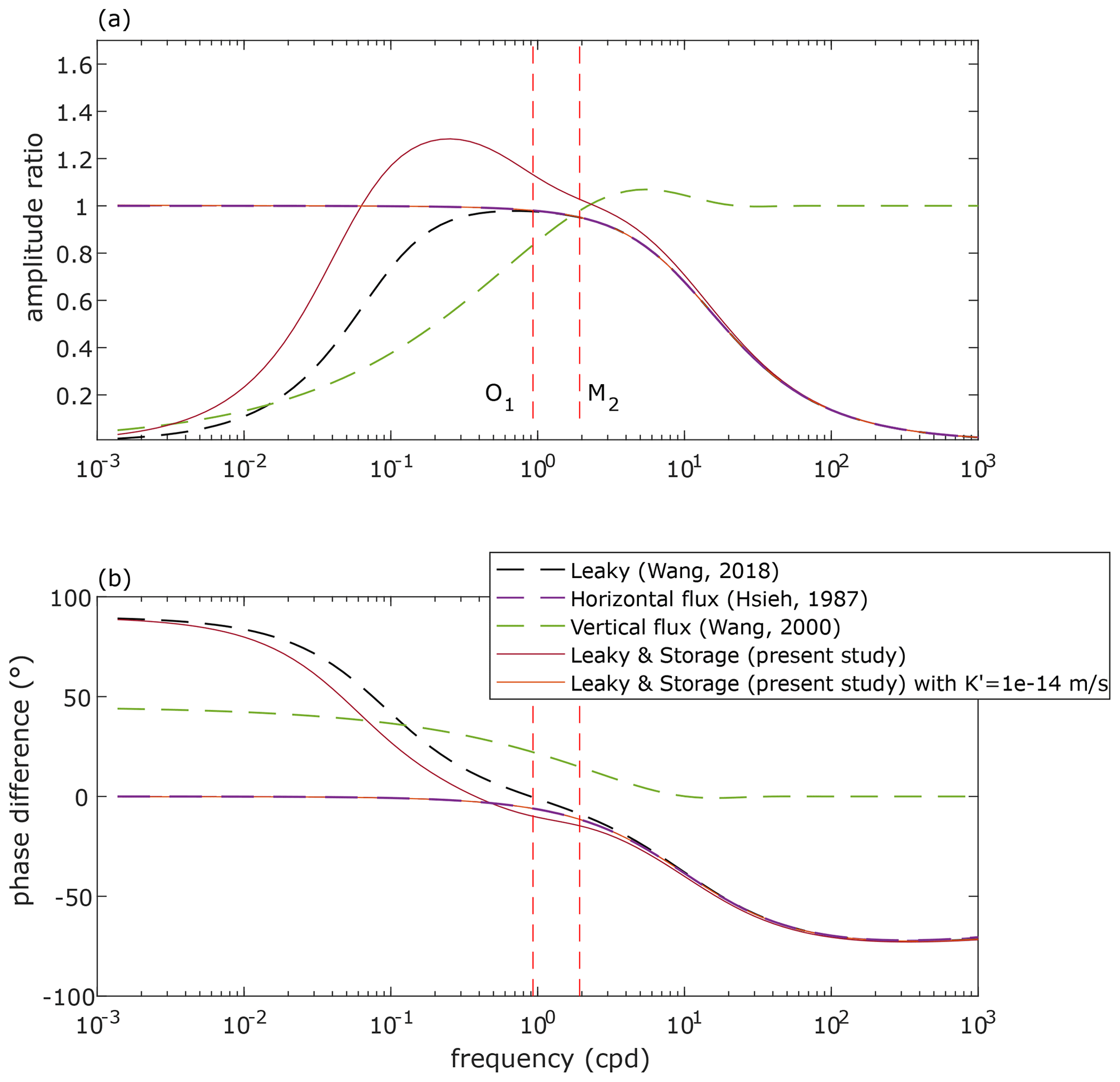
Figure 2 Frequency variation in amplitude response and phase shift in the groundwater response to Earth tides. The transmissivity (T) is 10⁻⁵ m² s⁻¹, storativity (S) is 10⁻⁴, hydraulic conductivity of the aquitard (K^′) is 10⁻⁸ m s⁻¹, aquitard hydraulic diffusivity (D^′) is 10⁻⁴ m² s⁻¹, the skin factor (sk) is 0, R_KuB is 1.4, the well casing radius (r_c) and screen radius (r_w) are 6.03 cm. b^′ was set to 5 m. Screen depth (z) was set to 23 m for the vertical-flow model of Wang (2000).

Because both horizontal and vertical flux models are associated with opposite phase shift signs (Fig. 2b), the latter can offer valuable insights for model selection (Allègre et al., 2014). Positive phase shifts in the vertical flux model are related to an increasing amplitude ratio with frequency, whereas the wellbore storage model exhibits the opposite behaviour. Wang et al. (2018) developed a leaky model capable of demonstrating both positive and negative phase shifts, where positive phase shifts correspond to an increasing amplitude ratio with frequencies and negative phase shifts are linked to a decreasing amplitude ratio.

Our new model showcases positive or negative phase shifts with an increasing or decreasing amplitude ratio over frequency, even allowing for amplitude ratios greater than 1. Notably, Wang (2000) observed a similar characteristic in the vertical flux model, with an amplitude just above 1 (1.06) for very specific conditions. At high frequencies, our model displays amplitude ratios and phase shifts similar to those of the leaky and wellbore storage models, reflecting the attenuation of high-frequency pore pressure fluctuations in the aquifer by well water.

At low frequencies (Fig. 2), the purely confined model exhibits a constant phase shift (0°) and amplitude ratio (Eq. 1). This constant behaviour is the signature of the absence of well impact on groundwater level fluctuations and the absence of phase shift between the Earth tide strain and the aquifer level fluctuations. It means that the groundwater fluctuations in the aquifer are the same as the groundwater fluctuations in the well (absence of amplification/attenuation and phase shifts) and that there is no phase shift between the strain and the water pressure variations inside the aquifer. For the “Leaky & Storage (present study)” model (Fig. 2), the leaky conditions do provoke a phase shift and an amplitude modification as compared to being purely confined. Such values of phase shift and amplitude modification do vary with frequency.

We explored the parameter space by focussing on the frequency-dependent amplitude response and phase shift responses for different sets of parameter values. The reference parameter set is the one described above. T, R_KuB, and z_i have a large impact on model shapes. As also observed by Hsieh et al. (1987), S does not have a major impact on the results (Fig. 3c and d). The skin effect does not play a large role in the useful frequency band (about 1 to 2 cpd, cycles per day) for amplitudes, but its influence is larger for the phase shifts when compared to the reference parameter set. K^′ does not significantly influence the results with respect to the reference parameter set used in the study (Fig. 3e to f). K^′ has the opposite role of S, and they appear to compensate each others' effects because of their respective role in Eq. (27).

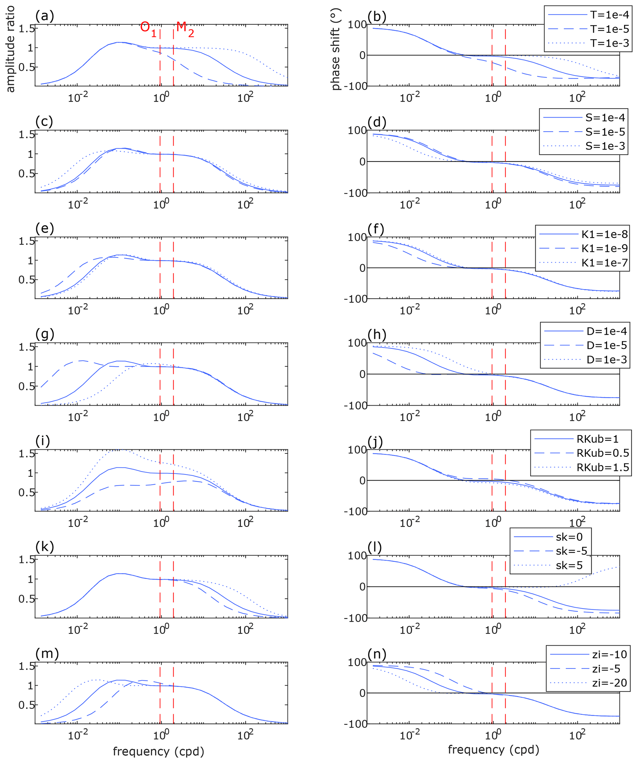
Figure 3 Illustration of the amplitude response (a, c, e, g, i, k, m) and phase shift (b, d, f, h, j, l, n) as a function of frequency for various parameters compared to the reference parameter set.

Figure 4 shows the impacts of considering leaky and skin effects for a realistic parameter set. Purely confined conditions (no leaky aquitard) do not create a phase shift between the volumetric strain in the aquifer (Fig. 4a) and the associated hydraulic head variation (Fig. 4b), while a compressible and leaky aquitard (Fig. 4b) or skin effects around the well (Fig. 4c) could involve positive phase shifts.

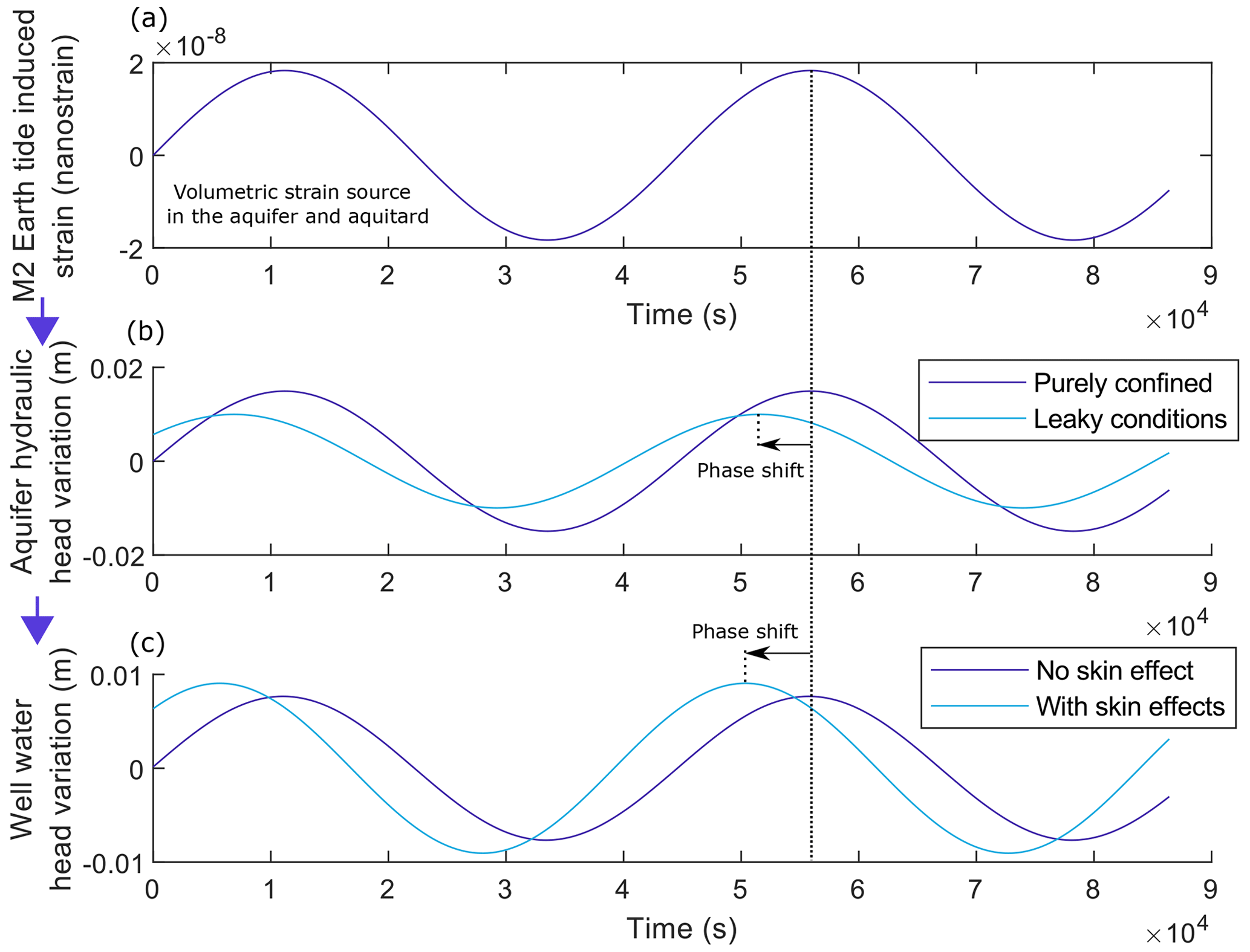
Figure 4 Example of the volumetric strain time series generated by the M₂ Earth tide in (a), which creates aquifer hydraulic head variations in (b), resulting in well water level variations in (c). The transmissivity (T) is 10⁻⁶ m² s⁻¹, storativity (S) is 7 × 10⁻⁴, hydraulic conductivity of the aquitard (K^′) is 10⁻⁶ m s⁻¹, aquitard hydraulic diffusivity (D^′) is 10⁻⁴ m² s⁻¹, the skin factor (sk) is −5 m, z_i is −10 m, R_KuB is 0.3, and the well casing radius (rc) and screen radius (rw) are 6.03 cm. B is set to 0.8 and K_u to 10 GPa.

3 Application of the new model to a groundwater monitoring dataset from Cambodia

3.1 Field site and previous results

The field site in northwest Cambodia comprises three boreholes drilled into the subsurface, consisting of mudstone, claystone, siltstone, and sandstone. Time series and pumping test results have been reported in Valois et al. (2022), while details of the lithology can be found in Vouillamoz et al. (2012, 2016) and Valois et al. (2017, 2018, 2022). Pumping from the aquifer is limited by a very low specific yield, attributed to the presence of fine deposits such as clay and mudstone (Vouillamoz et al., 2012; Valois et al., 2018).

The boreholes were drilled to a depth of 31 m with a radius of 0.1524 m and equipped with 0.1016 m. There is PVC casing from top to bottom, featuring a 9 m long screen at the hole's base. The aquifer is situated within a hard rock medium, comprising either claystone or sandstone, located beneath a 10 m thick clay layer.

For the pumping tests, the wells were pumped for 3 d, and water levels were allowed to recover for 4 d in two observation wells. The interpretation of the pumping tests utilized AQTESOLV^™/Pro v4.5 software, employing the leaky aquifer with aquitard storage model (Moench, 1985) or a 3D flow using the generalized radial flow model (Barker, 1988). The selected solutions, compared to other models (Theiss, Hantush, without aquitard storage), demonstrated the best fit with a root mean square error (RMSE) of 0.02 m for Cambodia.

3.2 Well sensitivities and phase shifts to Earth tides

Between 2010 and 2015, well water levels were measured at 20, 40, or 60 min intervals using absolute pressure sensors (Diver data loggers, Eijkelkamp Soil & Water, the Netherlands). To compensate for barometric pressure (BP) effects, data from a barometer located a few kilometres away from the field site were utilized (Eijkelkamp Soil and Water, the Netherlands). A zero-phase Butterworth filter was employed to eliminate low-frequency content (periods longer than 10 d) from both groundwater (GW) and BP data.

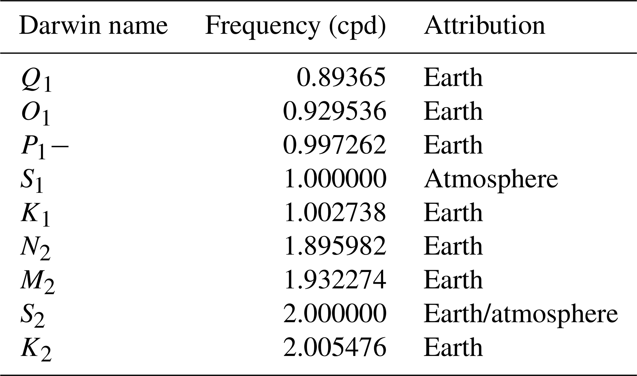
For each site's geolocation (latitude, longitude, and height), ET strain time series were computed at 20 min intervals using the SPOTL software (Agnew, 2012). The time series were then modelled using harmonic least squares (HALS; Schweizer et al., 2021) with eight frequencies corresponding to the major tides (Table 1) following Merritt's description (2004). HALS provides amplitude and phase estimations for each tidal component and record.

Table 1 Dominant tidal components that are generally found in groundwater measurements (adapted from MacMillan et al., 2019).

The results obtained from HALS were utilized to calculate the amplitude response and phase shift between GW and Earth tide (ET) for each tidal component. These amplitude responses are commonly known as “well sensitivities” to Earth tide strains (Rojstaczer and Agnew, 1989) and are summarized in Fig. 5 alongside the corresponding phase shifts.

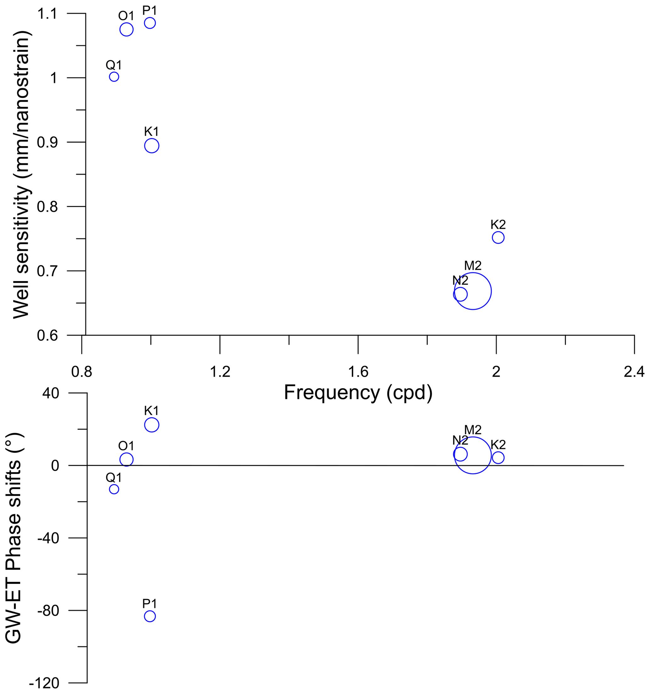
Figure 5 Amplitude responses and phase shifts as a function of frequency for the Cambodian site. S1 and S2 were excluded as they are not only generated by Earth tides. The circle size is proportional to the amplitude in the well water levels.

The well sensitivities to tides exhibit a frequency-dependent behaviour, resulting in similar values for neighbouring frequencies and a generally decreasing magnitude. The amplitudes of M₂ and N₂ are relatively straightforward to assess due to their significant magnitudes (11.2 and 2.1 mm respectively), and their amplitude responses and phase shifts are highly similar. The phase shifts for the tides of interest (O₁, N₂, and M₂) are positive. However, the signs of the amplitudes for the other tides can be attributed to their low-amplitude responses, which are challenging to characterize using HALS.

3.3 Fitting the $M_{\mathrm{2}}/O_{\mathrm{1}}$ amplitude response ratio and phase shifts

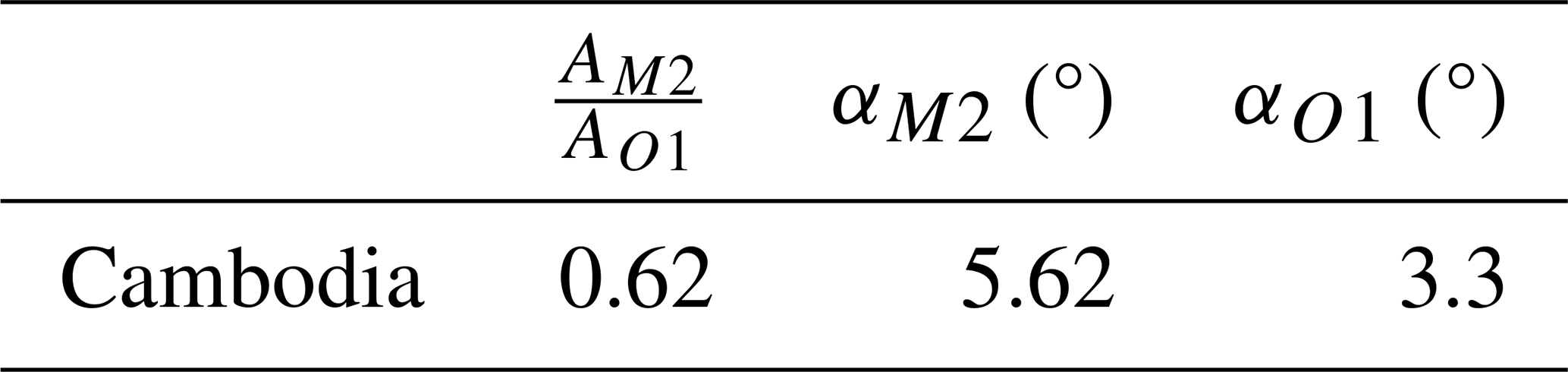
The analysis is restricted to two types of tides: the semi-diurnal and diurnal tides. This limitation arises because the magnitude of Earth-tide-induced well water levels is significantly damped for higher frequencies, making it difficult to discern and analyse tides beyond these two types. Here, we use amplitude responses (A_M2, A_O1) and phase shifts (α_M2, α_O1) to estimate hydraulic subsurface properties. The N₂ tide was not used since its response may be too similar to M₂ and does not help with constraining the model. Amplitudes are influenced by geomechanical parameters (BK_u) which are generally not considered in classical hydrogeology. Valois et al. (2022) previously illustrated that the M₂-to-O₁ amplitude response ratio can be computed because it is not directly multiplied by BK_u and because it provides useful information about model choice. This leads to a system of three equations and six parameters (T, S, K^′, D^′, skin, and R_KuB) by using the simplified model in Eq. (27) when the geometry of the well and the aquitard–aquifer system is known:

$$\begin{array}{}\text{(31)}& {\displaystyle \frac{A_{M\mathrm{2}}}{A_{O\mathrm{1}}}}=\left|h_{\mathrm{w},\mathrm{0},\mathit{\omega }={\mathrm{M}}_{\mathrm{2}}}/h_{\mathrm{w},\mathrm{0},\mathit{\omega }=O_{\mathrm{2}}}\right|,\text{(32)}& {\displaystyle }{\mathit{\alpha }}_{M\mathrm{2}}=\arg \left[h_{\mathrm{w},\mathrm{0},\mathit{\omega }={\mathrm{M}}_{\mathrm{2}}}/{\displaystyle \frac{B{K}_{\mathrm{u}}}{\mathit{\rho }g}}{\mathit{\epsilon }}_{\mathrm{0}}\right],\text{(33)}& {\displaystyle }{\mathit{\alpha }}_{O\mathrm{1}}=\arg \left[h_{\mathrm{w},\mathrm{0},\mathit{\omega }={\mathrm{O}}_{\mathrm{1}}}/{\displaystyle \frac{B{K}_{\mathrm{u}}}{\mathit{\rho }g}}{\mathit{\epsilon }}_{\mathrm{0}}\right].\end{array}$$

Table 2 displays the data to be fitted using the three equations above.

Table 2 Data to be fitted using the ET-GW model.

A systematic exploration of the entire parameter space without any constraints other than the well and aquifer geometry was carried out. Hydraulic and geomechanical property ranges are chosen according to the literature, i.e. De Marsily (1986) and Domenico and Schwartz (1998). In order to assess the goodness of fit with the three observed parameters (Eqs. 31 to 33), the objective chi-square function is defined below:

$$\begin{array}{}\text{(34)}& {\mathit{\chi }}^{\mathrm{2}}=\mathrm{1}/N{\sum }_{i=\mathrm{1}}^N{\left({\displaystyle \frac{({\mathrm{Obs}}_i-{\mathrm{Mod}}_i)}{{\mathrm{Error}}_i}}\right)}^{\mathrm{2}},\end{array}$$

where N is the number of observed parameters (3 here), Obs_i, Mod_i, and Error_i are the observed parameter, modelled parameter, and their errors respectively. Thus, this objective function takes into account errors in the observed parameters (De Pasquale et al., 2022). They were set to 0.1, 0.5° and 0.2 for α_M2, α_O1, and $\frac{A_{M\mathrm{2}}}{A_{O\mathrm{1}}}$ respectively, according to Valois et al. (2022).

The model allows us to fit both O₁ and M₂ positive phases and the low M₂-to-O₁ amplitude ratio (misfit close to 0 in Fig. 6), whereas the model of Gao et al. (2020) cannot do this (misfit above 1; see Appendix B and Valois et al., 2020). The T value is in good agreement with the pumping test range (Fig. 6a). S is 0.5 orders of magnitude below the pumping test range (Fig 6b), whereas the storativity best fit for Gao et al. (2020) is 2 orders of magnitude above (Appendix B). The skin effect also shows acceptable values as compared to the pumping test (Fig. 6f). The parameter exploration shows best fits for K^′ and D^′, whereas it is difficult to identify a clear best fit for the R_KuB parameter. The values are within the expected range for the hydrogeological configuration: the mudstone aquitard has a lower hydraulic conductivity (10⁻⁸ m s⁻¹) than the underlying claystone aquifer (coarser grain size than the aquitard, with a K value of about 10⁻⁷ m s⁻¹ for an aquifer thickness of 22 m) and a diffusivity of about 10⁻⁴ m² s⁻¹. This is in agreement with the aquitard classification of Pacheco (2013).

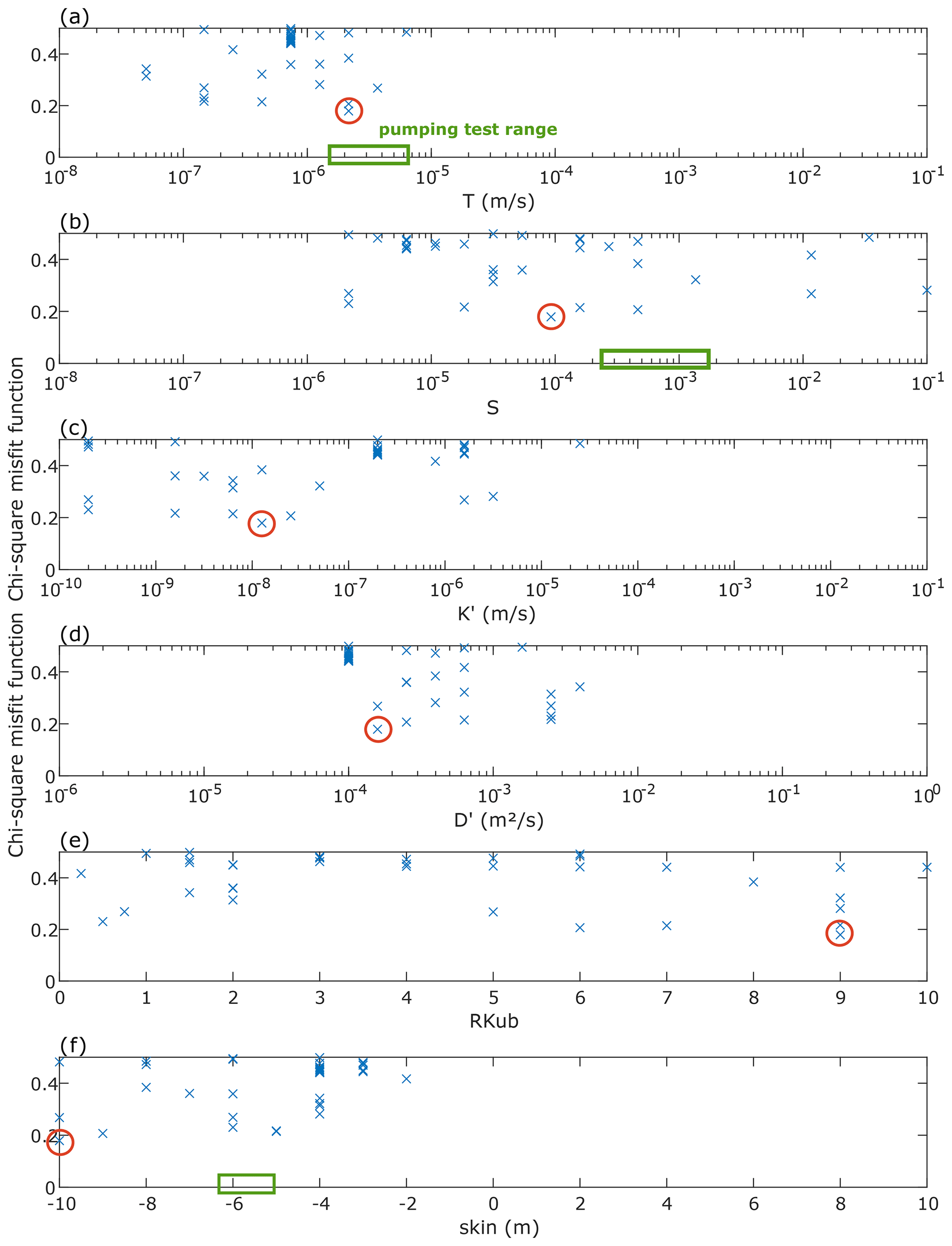
Figure 6 Results of full parameter exploration using the leaky-with-storage aquifer model for the Cambodian case study. Red circles represent the best fit.

4 Discussion

4.1 Uncertainties and discrepancies

There are several sources of uncertainty which originate from measurement and their propagation as well as uncertainties introduced by model assumptions. We believe that uncertainties linked to pressure sensor resolution (0.2 mm) and time resolution (20 min) as well as the HALS decomposition were too low to be worth considering, at least for the semi-diurnal tides. This can be deduced from the nearly identical amplitude responses at M₂ and N₂ at our field site. Because those responses are indeed identical, it means that errors in the raw dataset did not influence the response characterization. We note that amplitude responses and phase shifts show larger discrepancies for the diurnal tides. This could be linked to overall lower amplitudes which are generally more difficult to characterize. We therefore conclude that errors arising from uncertainties are negligible compared to the uncertainty introduced by model assumptions, in agreement with Sun et al. (2020).

Discrepancies between hydro-geomechanical properties derived from the groundwater response to Earth tides (termed “passive” and assuming a compressible matrix) and hydraulic testing (e.g. slug, pump and lab testing, termed “active” and generally assuming an incompressible matrix) have been reported in the literature and have not been appropriately reconciled. By fitting the amplitude response ratio and phase shifts (Sect. 3.3), a T value discrepancy of 1 order of magnitude can be observed between both approaches. We hypothesize that this is caused by parameter anisotropy.

Zhang et al. (2019b) pointed out differences in hydraulic conductivities of more than 1 order of magnitude between ET analysis and slug tests and attributed this to differences in the investigated scale. Allègre et al. (2016) reported much higher values of storativity derived from pumping test as compared to ET when using the vertical-flow model. Sun et al. (2020) showed that T values are frequency-dependent with differences of several orders of magnitude when comparing co-seismic, ET, and slug or pump test methods. The discrepancies can be explained by the different conceptual models used in the active (based on perfectly confined conditions) and passive methods (based on leaky conditions) or by the frequency dependency of hydraulic parameters. The literature illustrates that transmissivity, hydraulic conductivity, or specific storage can indeed vary depending on the frequency of the forcing (e.g. Cartwright et al., 2005; Renner and Messar, 2006; Guiltinan and Becker, 2015; Rabinovich et al., 2015). This demonstrates the need for attention when assessing hydraulic parameters using passive methods for semi-confined conditions. We specifically emphasize the need to use the same conceptual model (i.e. confined, leaky with or without storage, vertical flow) when comparing active and passive methods, as well as the need for preliminary hydrogeological knowledge of both the aquifer system (i.e. presence of an aquitard with or without storage) (Bastias et al., 2022) and the borehole skin effect.

4.2 The use of the leaky model with aquitard storage

Our new analytical solution describing the well water level response to harmonic Earth tide strains contains at least six hydro-geomechanical parameters that could be derived from only three features, e.g. the M₂-to-O₁ amplitude response ratio and M₂ and O₁ phase shifts. Applying this model to real-world cases to derive properties from amplitude responses and phase shifts provides relevant information on T, S, D^′, K^′, and the skin effect, but it is prone to non-uniqueness. Thus, a priori information may be needed depending on the capacity of the inverse problem to fit observed data (phases shifts and amplitude ratio). In our case study, parameter assessment would benefit from prior information on S (or K^′) and R_KuB.

The model presented in this study can be useful when the hydrogeological configuration involves storage in the aquitard with fixed head (i.e. Dirichlet) boundary conditions and for cases where phase shifts and amplitude ratio do exemplify a specific pattern. For example, when compared to Gao et al. (2020) and using the parameterization of the present study (Fig. 7), our solution is able to model lower a M₂-to-O₁ amplitude ratio, lower phases, and a higher amplitude ratio for phases close to 0.

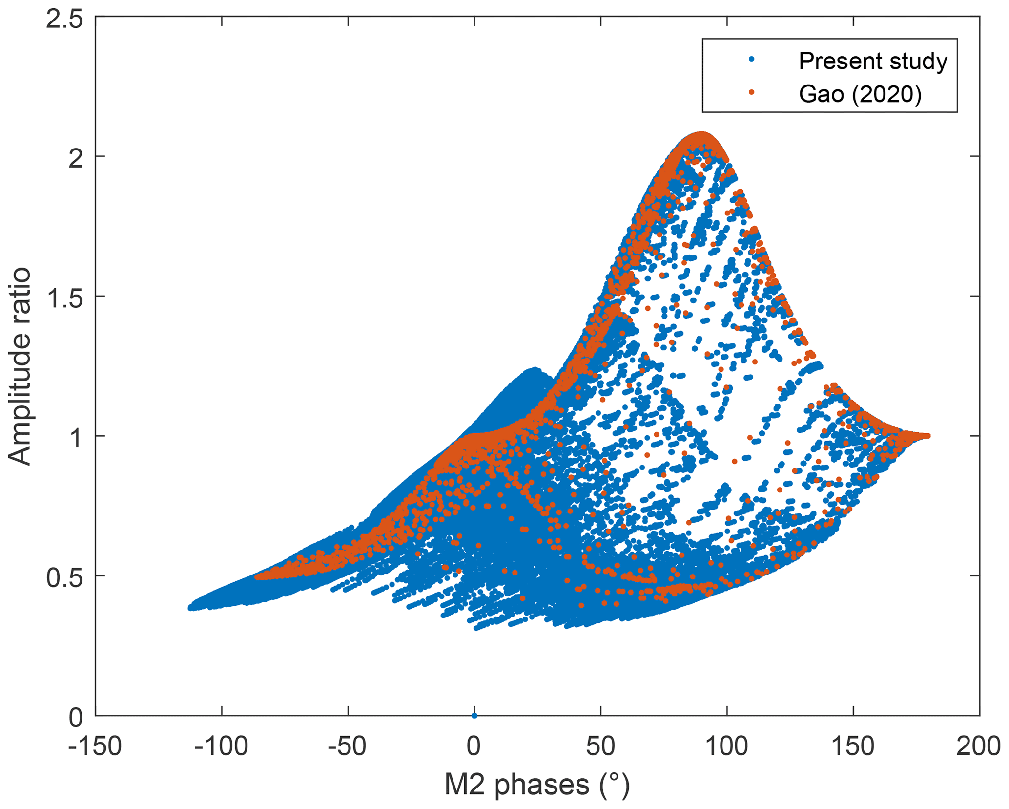
Figure 7 Outputs of the models using the parameterization of the study (rc = rw = 6.08 cm, z_i=-10 m).

While the amplitudes are controlled by the product of the Skempton coefficient and the undrained bulk modulus, these mechanical parameters also affect phase shifts. Therefore, further investigations are needed to assess these influences using other methods or to link them empirically with the hydraulic parameters. This is crucial to enhance confidence in utilizing the groundwater response to Earth tides as a valuable tool for better understanding and characterizing groundwater resources.

5 Conclusions

We have developed a new analytical solution for the well water level response to Earth tide strains. This solution considers a previously unprecedented physical reality, specifically, a leaky aquifer with aquitard storage, subject to Dirichlet boundary conditions under tidal strain. Additionally, our model considers the influence of borehole storage and skin effects, further improving the accuracy and comprehensiveness of the analysis. This model extends upon previous models and allows advanced characterization of the subsurface using the groundwater response to natural forces. The new model overcomes previous limitations, for example it explains very low M₂-to-O₁ amplitude ratios as well as a large phase shift difference between M₂ and O₁ tides. The model relies on six combinations of hydro-geomechanical parameters. In this study, we assess the most sensitive parameters to be the transmissivity, the well skin effect, the aquitard-to-aquifer mechanical parameter ratio ($B^{\prime }{K}_{\mathrm{u}}^{\prime }/B{K}_{\mathrm{u}}$), and the aquitard diffusivity and aquitard-conductivity-to-aquifer-storativity ratio.

We apply our new model to a groundwater monitoring dataset from Cambodia and compare the results with pumping tests undertaken in the same formation. We used the diurnal (O₁) and semi-diurnal (M₂) tides to better constrain the model. Results illustrate significant insight into subsurface properties. For example, we derive relevant information about T, S, D^′,K^′, and the skin effect, when compared to the pumping test results. Overall, our new model can be used to shed light on previously inexplicable well water level behaviour and can be paired with other investigation methods to enhance the understanding of subsurface processes.

Appendix A: The analytical solution in the aquitard

To solve Eq. (14) with the boundary conditions in Eqs. (7) and (8), we define

$$\begin{array}{}\text{(A1)}& {\widehat{h}}_{\mathrm{0}}^{\prime }=h_{\mathrm{0}}^{\prime }-{\displaystyle \frac{B^{\prime }{K}_{\mathrm{u}}^{\prime }}{\mathit{\rho }g}}{\mathit{\epsilon }}_{\mathrm{0}}.\end{array}$$

Thus, the equation system becomes

$$\begin{array}{}\text{(A2)}& {\displaystyle }\left({\displaystyle \frac{{\partial }^{\mathrm{2}}{\widehat{h}}_{\mathrm{0}}^{\prime }}{\partial z^{\mathrm{2}}}}\right)={\displaystyle \frac{i\mathit{\omega }{\widehat{h}}_{\mathrm{0}}^{\prime }}{D^{\prime }}},\text{(A3)}& {\displaystyle }{\widehat{h}}_{\mathrm{0}}^{\prime }\left(z=z_{\mathrm{i}}\right)=h_{\mathrm{0}}-{\displaystyle \frac{B^{\prime }{K}_{\mathrm{u}}^{\prime }}{\mathit{\rho }g}}{\mathit{\epsilon }}_{\mathrm{0}},\text{(A4)}& {\displaystyle }{\widehat{h}}_{\mathrm{0}}^{\prime }\left(z=\mathrm{0}\right)=h_j^{\prime }-{\displaystyle \frac{B^{\prime }{K}_{\mathrm{u}}^{\prime }}{\mathit{\rho }g}}{\mathit{\epsilon }}_{\mathrm{0}}.\end{array}$$

The solution ${\widehat{h}}_{\mathrm{0}}^{\prime }$ is of the following form:

$$\begin{array}{}\text{(A5)}& {\widehat{h}}_{\mathrm{0}}^{\prime }=A_{\mathrm{1}}{e}^{\frac{\left(\mathrm{1}+i\right)}{\mathit{\delta }}(z-z_{\mathrm{i}})}+A_{\mathrm{2}}{e}^{-\frac{\left(\mathrm{1}+i\right)}{\mathit{\delta }}(z-z_{\mathrm{i}})}.\end{array}$$

It yields

$$\begin{array}{}\text{(A6)}& {\displaystyle }{A}_{\mathrm{1}}={\displaystyle \frac{e^{\frac{\left(\mathrm{1}+i\right)}{\mathit{\delta }}{z}_{\mathrm{i}}}\left(h_{\mathrm{0}}-\frac{B^{\prime }{K}_{\mathrm{u}}^{\prime }}{\mathit{\rho }g}{\mathit{\epsilon }}_{\mathrm{0}}\right)-(h_j^{\prime }-\frac{B^{\prime }{K}_{\mathrm{u}}^{\prime }}{\mathit{\rho }g}{\mathit{\epsilon }}_{\mathrm{0}})}{\mathrm{2}\sin h\left(\frac{\left(\mathrm{1}+i\right)}{\mathit{\delta }}{z}_{\mathrm{i}}\right)}},\text{(A7)}& {\displaystyle }{A}_{\mathrm{2}}={\displaystyle \frac{-e^{-\frac{\left(\mathrm{1}+i\right)}{\mathit{\delta }}{z}_{\mathrm{i}}}\left(h_{\mathrm{0}}-\frac{B^{\prime }{K}_{\mathrm{u}}^{\prime }}{\mathit{\rho }g}{\mathit{\epsilon }}_{\mathrm{0}}\right)+(h_j^{\prime }-\frac{B^{\prime }{K}_{\mathrm{u}}^{\prime }}{\mathit{\rho }g}{\mathit{\epsilon }}_{\mathrm{0}})}{\mathrm{2}\sin h\left(\frac{\left(\mathrm{1}+i\right)}{\mathit{\delta }}{z}_{\mathrm{i}}\right)}}.\end{array}$$

Thus,

$$\begin{array}{}\text{(A8)}& h_{\mathrm{0}}^{\prime }=A_{\mathrm{1}}{e}^{\frac{\left(\mathrm{1}+i\right)}{\mathit{\delta }}(z-z_{\mathrm{i}})}+A_{\mathrm{2}}{e}^{-\frac{\left(\mathrm{1}+i\right)}{\mathit{\delta }}(z-z_{\mathrm{i}})}+{\displaystyle \frac{B^{\prime }{K}_{\mathrm{u}}^{\prime }}{\mathit{\rho }g}}{\mathit{\epsilon }}_{\mathrm{0}}.\end{array}$$

Appendix B: Additional information on parameter exploration

Figure B1 shows the misfit functions using the model developed in this study and the model of Gao et al. (2020). Misfits are clearly higher for the older model, which does not consider storage and tidal response in the aquitard. The storativity best fit using the model of Gao et al. (2020) failed to reproduce pumping test values. Nevertheless, transmissivity and skin estimates fall within the pumping test range.

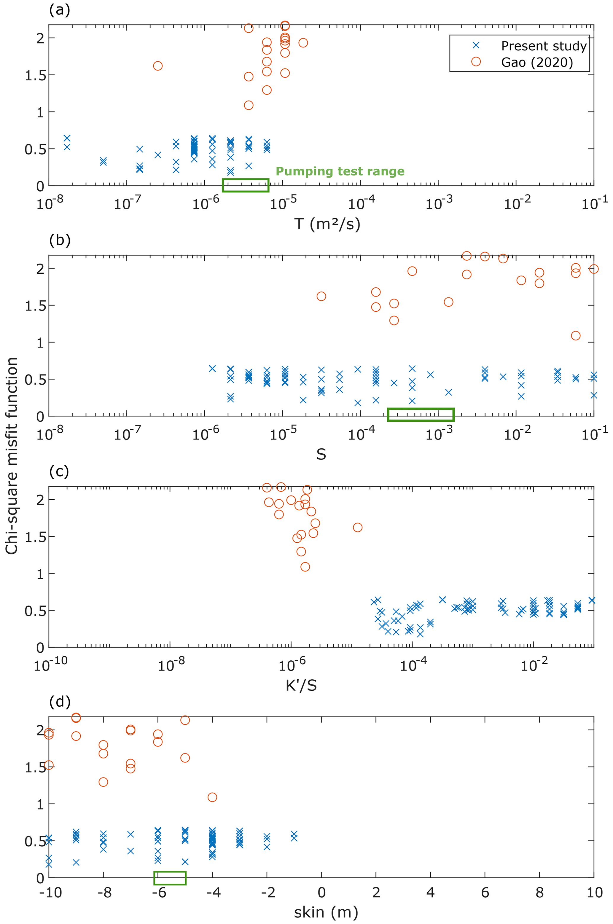
Figure B1 Comparison of misfit function for the present model and the one of Gao et al. (2020) for the Cambodian case study. Only the first hundred best fits were plotted.