the Creative Commons Attribution 4.0 License.
the Creative Commons Attribution 4.0 License.
 | 09 Feb 2023
Signal contribution of distant areas to cosmic-ray neutron sensors – implications for footprint and sensitivity
Markus Köhli
Steffen Zacharias
This paper presents a new theoretical approach to estimate the contribution of distant areas to the measurement signal of cosmic-ray neutron detectors for snow and soil moisture monitoring. The algorithm is based on the local neutron production and the transport mechanism, given by the neutron–moisture relationship and the radial intensity function, respectively. The purely analytical approach has been validated with physics-based neutron transport simulations for heterogeneous soil moisture patterns, exemplary landscape features, and remote fields at a distance. We found that the method provides good approximations of simulated signal contributions in patchy soils with typical deviations of less than 1 %. Moreover, implications of this concept have been investigated for the neutron–moisture relationship, where the signal contribution of an area has the potential to explain deviating shapes of this curve that are often reported in the literature. Finally, the method has been used to develop a new practical footprint definition to express whether or not a distant area's soil moisture change is actually detectable in terms of measurement precision. The presented concepts answer long-lasting questions about the influence of distant landscape structures in the integral footprint of the sensor without the need for computationally expensive simulations. The new insights are highly relevant to support signal interpretation, data harmonization, and sensor calibration and will be particularly useful for sensors positioned in complex terrain or on agriculturally managed sites.
- Article
(5277 KB) - Full-text XML
-
Supplement
(559 KB) - BibTeX
- EndNote


Cosmic-ray neutron sensing (CRNS) is an established measurement technique for water content in soils and snow (Andreasen et al., 2017b). The high integration depth and the large measurement footprint have been shown to provide an important advantage for field-scale applications compared to conventional point-scale sensors. However, the intrinsic integration over the whole footprint volume conceals the individual contributions of different patches and may result in biased observations (Franz et al., 2013; Schrön et al., 2018a; Schattan et al., 2019).
The footprint was initially characterized by its radius of around 300 m by Zreda et al. (2008) and Desilets and Zreda (2013) without significant dependency on soil moisture or air humidity. Later, Köhli et al. (2015) revisited the physical assumptions of the underlying neutron simulations and proposed a moisture-dependent footprint radius in the range from 130 to 240 m. Besides the epithermal neutron transport, also thermal neutron footprints were investigated by Jakobi et al. (2021).
These studies take into account the high complexity of neutron transport physics, which usually can only be investigated with computationally expensive Monte Carlo simulations. The accepted definition of the epithermal footprint radius, R86, covers the % quantile of detected neutrons. This measure was introduced by Desilets and Zreda (2013) and has been inherited by Köhli et al. (2015) in order to maintain consistency. However, the definition involves four problematic aspects: (i) the radial intensity function, Wr(h,θ), does not follow a simple exponential shape (Köhli et al., 2015; Schrön et al., 2017). Therefore, the 1−e−2 limit may be misleading when it is used to draw conclusions about the intensity–radius relationship elsewhere. (ii) High-quantile values for strongly non-linear functions may overestimate the long-range influence of neutrons, regardless of how often and where they have probed the soil. (iii) The fact that the definition of the footprint has been developed for homogeneous situations increases the uncertainty and complicates the interpretation in more heterogeneous and more complex terrain. And (iv), the definition hardly allows us to investigate problems and questions that often arise during practical applications: is the detector sensitive to remote soil moisture changes? Does a certain patch of the area influence the detector signal and by how much?
As a standard solution for such questions, neutron transport physics-based Monte Carlo codes could be employed with detailed modelling of the local conditions (as has been done by e.g. Franz et al., 2013; Köhli et al., 2015; Schrön et al., 2018a; Schattan et al., 2017; Li et al., 2019). However, this technique is impractical for quick assessments and mostly limited to scientific applications.
While cosmic-ray neutron sensors are usually employed to track soil moisture changes in the area of their footprint, complex structures or heterogeneous patterns in the footprint may influence the measurement undesirably. The dependency of the measured neutrons on soil moisture changes has been originally expressed by the neutron–moisture relationship (Desilets et al., 2010; Köhli et al., 2021) and has also been adapted for snow (Schattan et al., 2017). Many natural sites are highly heterogeneous, and thus knowledge of the contribution of distant areas to the measurement signal would be very useful, e.g. to support calibration sampling, sensor location design, data interpretation, and uncertainty assessment. Typical events modulating water abundance and distribution are, for example, land management activities like harvesting (Franz et al., 2016; Tian and Song, 2019), ploughing (Kasner et al., 2022), and irrigation (Li et al., 2019; Ragab et al., 2017), as well as natural events like rainwater interception in forests (Baroni and Oswald, 2015; Andreasen et al., 2017a; Schrön et al., 2017), snowmelt and redistribution (Schattan et al., 2019), or different soil dry-out rates due to different soil hydraulic conductivity (Scheiffele et al., 2020).
In the past, spatially (and temporally) variable factors within the footprint influencing the neutron signal have often been identified as the source of unexplained features in the data. These discoveries sometimes boosted scientific insights on neutron transport and even led to more reliable hydrological data (see e.g. Bogena et al., 2013; Schrön et al., 2017, 2018a; Schattan et al., 2019; Rasche et al., 2021). However, at most heterogeneous sites CRNS calibration and validation remains a challenge, since the influence of the differing structures or patches in the footprint to the signal is usually not known (Coopersmith et al., 2014; Lv et al., 2014; Iwema et al., 2015; Franz et al., 2016; Heistermann et al., 2021). For this reason, many authors have reported differing shapes of the neutron–moisture curve and have conducted site-specific empirical reparameterizations to fit their data (Rivera Villarreyes et al., 2011; Lv et al., 2014; Iwema et al., 2015; Heidbüchel et al., 2016). Others developed directional sensors to focus the measurement only on specific parts of the landscape (Francke et al., 2022), which remains a technological challenge on its own.
One way to approach the estimation of signal contributions of different areas in the footprint is to use the radial intensity function Wr. First attempts to realize this idea were performed by Schrön et al. (2017), who improved the sensor calibration by applying different weights to areas depending on size, distance, and land-use class, and also by Schrön et al. (2018a), who excluded the contribution of a concrete area around a grassland site in order to improve reliability of soil moisture dynamics measured by stationary CRNSs.
In the present study we aim at generalizing this concept for typical combinations of heterogeneous land-use and soil moisture patterns. Our hypothesis is that the contribution to the detector signal of various complex areas in the footprint can be estimated analytically based on the existing theories about neutron production and transport. The first section will describe the proposed approach and discuss its potential limitations. Then, the method will be evaluated by dedicated neutron transport simulations for various scenarios of different soil moisture patterns, land-use types, and geometries. We further aim at exploring two applications of this concept: first, to assess its explanatory power for the shape of the neutron–soil–moisture relationship and, second, to provide a more practical footprint definition expressing whether or not a distant area's soil moisture change (e.g. by irrigation or rainwater interception, or faster drainage) is actually visible to the neutron signal in terms of measurement precision.
2.1 The radial intensity function
The sensitivity of a central detector to an infinitesimal ring at distance r was described by Köhli et al. (2015) and refined by Schrön et al. (2017) as
which is a combination of two exponential functions with factors and slopes () that represent the complex nature of neutron transport in homogeneous environments. This radial intensity function Wr (see Fig. 1a) depicts the number of detected neutrons that originated in the soil at the distance r (in m) under certain homogeneous conditions of air humidity h, (soil) water equivalent θ, air pressure P, and vegetation height Hveg. It can also be expressed as with being scaled by air pressure and vegetation influence (see Schrön et al., 2017, for the details). We use this simplified formulation in the following, while results can be easily transferred to other pressure and vegetation conditions by rescaling r as mentioned.
An alternative parameterization, , was proposed by Schrön et al. (2017) as an approximation for average humidity and soil moisture conditions:
This approximation can be evaluated in a computationally more efficient way, as it does not depend on humidity and soil moisture, but at the same time it is less accurate towards the extreme ends of dry or wet conditions.
The integral of Wr(h,θ) over all radii r represents the total number of detected neutrons, N:
In other words, the detectable neutron intensity at the centre of the radial footprint is the sum of all the ring intensities, Wr, across the whole domain Ω.
Based on this definition, Köhli et al. (2015) derived the hitherto accepted CRNS footprint radius, R86, as the distance within which 86 % of all the detected neutrons originated:
2.2 The concept of signal contributions from sub-domain areas
Let Ai∈Ω be a set of sub-domain areas with water content θi, constituting the whole domain Ω (see Fig. 2 for an exemplary illustration). We propose that the total measured neutron intensity at the centre, or effective neutron intensity , is the sum of all the neutrons which were generated in Ai, weighted by their ability to reach the sensor, i.e.
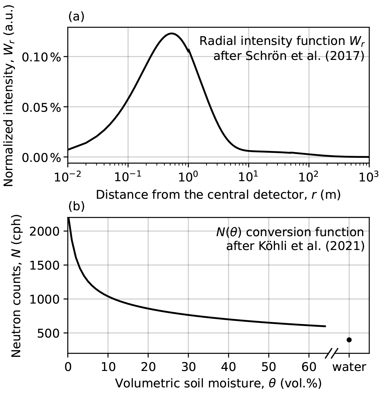
Figure 1Basic functions of CRNS theory. (a) The radial intensity function, , representing the intensity contribution of all points at distance r to the detector signal. (b) The conversion function, , for a typical stationary CRNS sensor.
This quantity can be expressed as the product of the locally generated neutrons, Ni=N(θi), and the radial intensity weight of its area, wi. The total signal then is
In a homogeneous domain, where , the integral weight wi of an arbitrary subset area Ai directly represents the area's contribution to the measured neutron signal, only depending on size and distance. In an inhomogeneous scenario, the contribution also depends on the local count rate Ni. For example, the effective signal of a symmetrical domain containing two identical half-spaces with a sensor in the centre would be an equal combination of the individual intensities, .
The relative contribution ci of the area Ai to the sensor signal is particularly useful for inhomogeneous, i.e. patchy scenarios and can be expressed as
In the above example, the relative contribution of the field 1 would be .
The proposed method can be applied to an arbitrarily complex combination of areas Ai.
The weight of the areas could be determined in two ways. In an angular environment, the integral over Ai could span the respective range of angles and radii (see Schrön et al., 2018a, Sect. 3.5):
In gridded environments, the spatial integral is simply the sum of the weights over all grid cells (see Schrön et al., 2017, Sect. 2.3):
For computational implementations, it is often easier to perform calculations on Cartesian coordinate systems (the latter option), such that the individual weight of each grid cell follows . Here, r is the distance between the detector and the centre of a grid cell, and Wr is the radial intensity at this distance. As for all numerical approximations, the size of the grid cell should be small compared to relevant structures in the footprint.
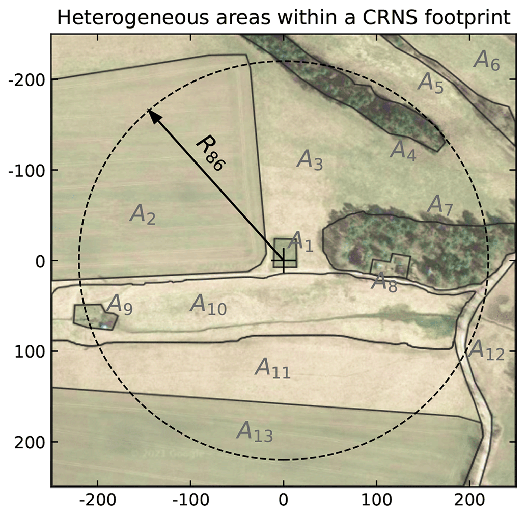
Figure 2Exemplary scenario of the site “Schäfertal” (51.6551∘ N, 11.0525∘ E; Wollschläger et al., 2017). Relevant areas Ai within the footprint of the central CRNS detector (+) are indicated by black borders, e.g. the agricultural land (A2, A13), forest sites (A4, A7), buildings (A8, A9), or the river creek (A10). The dashed circle illustrates the conventional footprint definition, R86, within which 86 % of detected neutrons probed the soil. (Satellite image © Google Maps.)
2.3 Potential limitations and remarks
The simplified approach cannot claim to be able to simulate the complex physics of neutron transport for every possible scenario. Just from the way it is formulated, some potential limitations of this approach can be expected already. The performance tests in the present study aim at challenging some of these objections with synthetic examples and evaluations by Monte Carlo simulations.
A direct limitation is that Wr has been initially defined as a radially symmetric function, assuming equal contribution at distances r in all directions. However, most heterogeneous regions are not radially structured such that highly variable soil moisture patches would lead to asymmetric weights in different directions, giving the corresponding footprint radius an amoeba-like shape (see e.g. Köhli et al., 2015; Schattan et al., 2019, Figs. 9 and 9, respectively).
The Wr function has also been derived for homogeneous conditions, and thus sharp borders of soil moisture patterns may not be resolved adequately. This is particularly true in regions of high sensitivity, such as the first few metres below and around the detector. These cases could lead to road-effect-like biases (Schrön et al., 2017, 2018b) and should be avoided in realistic applications.
Moreover, the actually detected neutron flux at the centre not only depends on the neutron response of all the individual fields but also on secondary interactions with water and soil between the detector and the remote field. These intermediate fields may influence the neutron's travel path and moderation probability, since neutrons typically undergo several interactions with the soil on their way to the detector (Köhli et al., 2015).
The approach also treats each area individually and cannot reproduce spatial interaction effects. They can occur when neutrons generated in an area typically diffuse to nearby areas, influencing their apparent local neutron intensity (see e.g. Schrön et al., 2018a). For this reason, scenarios in this study will exhibit sufficient space between distinct areas such that their neutron contribution can be assessed individually.
When it comes to evaluation of the presented approach with measurement data, it should be noted that results obtained from Wr-based approaches, as well as from URANOS particle origins, only represent detected neutrons with preceding soil contact, while a considerable fraction of the CRNS-measured signal is direct radiation from incoming neutrons (see Schrön et al., 2016, Fig. 3). This additional signal component is usually rather constant but could lead to a slightly lower magnitude of signal contributions in real-world examples.
It is briefly noted that a similar analysis could also be conducted for vertical footprints, i.e. the sensor's penetration depth. For example, the question, at which depth groundwater rise is visible to the CRNS, could be answered by similar methods as described above, using the depth-weighting function Wd instead of Wr (Schrön et al., 2017). However, neutrons undergo many more interactions in the soil on their way to the detector, in strong contrast to horizontal transport, such that we suspect this endeavour to be less promising, especially for strong vertical soil moisture profiles.
2.4 Conversion between neutrons and soil moisture
The measured neutron count rate N of a CRNS sensor is usually estimated with a neutron–moisture relationship N(θ), where θ is the soil water content in the homogeneous sensor footprint. In this study, we postulate that this relationship can also be used to calculate the neutron intensity of each fractional area in the footprint individually (see Fig. 1b). Furthermore, we propose to estimate the effective soil moisture product, , by assuming an equally mixing neutron gas at the centre of the footprint, , given by Eq. (6):
This is not a trivial assumption, especially for heterogeneous regions, where the average (i.e. effectively measured) soil moisture may often be biased towards drier areas due to the non-linearity of this relationship. The terms N(θ) and θ(N) depict the conversion functions used to derive neutrons from soil moisture and the other way round, respectively. In this study, we use the updated version of this relationship developed by Köhli et al. (2021) (Fig. 1b) which also depends on air humidity and better follows standard simulation results than the equation from Desilets et al. (2010):
where N0 is a detector-specific scaling parameter (here: 1950 cph), h is the air humidity (here: 5 g m−3), and p1…8=(0.0226, 0.207, 1.024, −0.0093, 0.000074, 1.625, 0.235, −0.0029) is the parameter set “uranos drf” from Köhli et al. (2021), which employs an energy-dependent detector response function (drf) for typical CRNS configurations (Köhli et al., 2018). For the case of pure water, this equation reduces to .
2.5 Physical neutron transport simulations
Neutron transport simulations were employed using the Monte Carlo code URANOS (Köhli et al., 2023). The model setup was generated with standard layers and parameters, such as an air pressure of 1013 hPa, a vertical cut-off rigidity of 5 GV, a domain size of 1000×1000 m2, and a central cylindrical detector with 9 m radius. The detector size is just a numerical parameter, typically used to reduce the computational effort, and will have no impact on the results if the area below the detector is kept homogeneous. Neutron origins were counted as the location of the first non-air contact of a detected neutron.
Water content has been added to various regions in the ground layer in order to resemble the investigated soil moisture patterns. However, soil directly below and in the immediate vicinity of the detector has been kept homogeneous, because the detector cannot resolve structures below its own extent. Modelled materials include soil with 50 % porosity, water (1 g cm−3), concrete (2 g cm−3), and in some cases an additional above-ground layer of 20 m height containing a uniform mixture of gas to represent forests or houses. The “house gas” mimics air surrounded by cement walls with soil-like material (0.15 kg m−3, 10 % water), and the “tree gas” represents cellulose with 3 kg m−3. The input material definitions for all scenarios are listed in the Supplement; see also Köhli et al. (2023) and their URANOS code repository for more details.
3.1 Heterogeneous soil moisture patterns
In order to provide a reliable representation of the average soil moisture in a heterogeneous domain, it is necessary to consider the specific soil moisture conditions of each individual area. We challenge the presented approach with complex soil moisture patterns that are designed to cover difficult aspects of neutron transport for the test.
Figures 3 and 4 show soil moisture distributions at 1000 and 500 m scales, respectively. The different areas are arranged such that fields that would theoretically contribute equally to the sensor (due to the same size, distance, and water content) still require their neutrons to pass other fields on their way to the detector that has much different soil moisture. The two different scales of the domain are also chosen to investigate the long-range (distance to corner: r<707 m) and short-range (r<354 m) performance of the analytical approach.
Figures 3a and 4a indicate the soil moisture pattern at the different domain scales, while the conventional footprint radius R86 is indicated by a dashed line. Based on these hypothetical distributions of soil moisture, the individual contributions ci of each area to the neutron signal at the centre (0,0) have been calculated following Eq. (7), with the results presented in Figs. 3b and 4b. It is clearly visible that the area with θ=20 vol % has the highest contribution to the signal, since it covers the direct vicinity of the detector in the centre and also most of the remaining fields. As expected and in accordance with the theory, the highest contribution is evident for areas that are closer to the detector and drier than others.
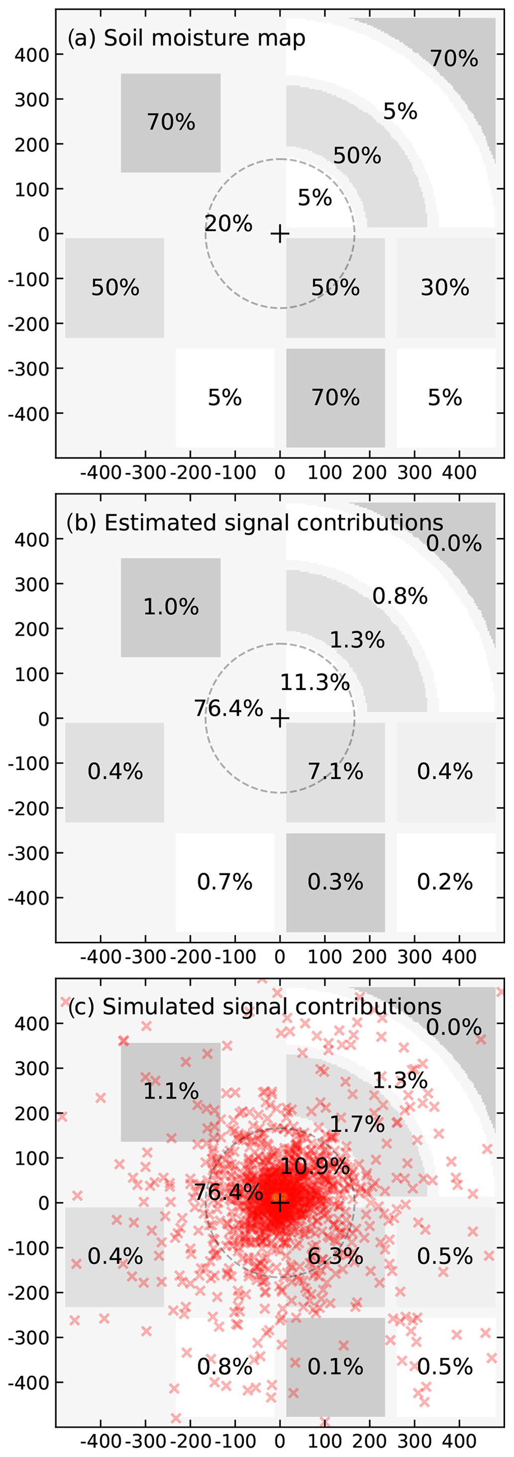
Figure 3Scenario 1000×1000 m with (a) a complex soil moisture pattern (grey scale); see also Fig. 7 for details. (b) Contribution to the detector signal estimated with the analytical method and (c) simulated with URANOS.
We briefly showcase the calculation of the contribution of an exemplary area A, e.g. the bent field with θA=50 vol % in the upper right quadrant of Fig. 4. To compute the weight of the area, one can either weight each grid cell i of the matrix with and sum it up or integrate Wr from radii r1=98 m to r2=167 m and from angles to . The last option is easier for radial geometries. The integration over the radii gives 0.118 for the radial weight of a full circular ring (relative to the total weight of the domain, ∫ΩWr), while the angular weight of the circular section equals . This results in the normalized spatial weight of %. It would already be the sought contribution to the detector signal if the domain was homogeneous. In this heterogeneous example, however, the spatial weight needs to be multiplied by the neutrons produced by this area, cph, and normalized by the effective count rate measured in the centre, cph, resulting in a contribution of % to the detector signal.
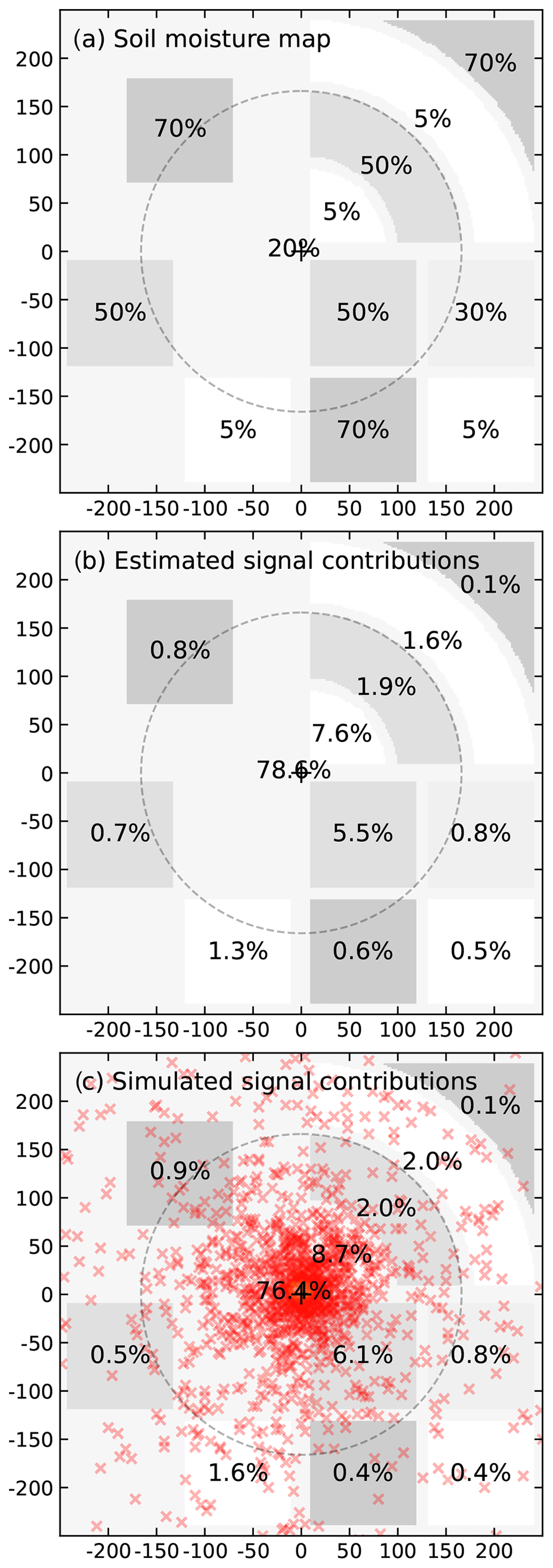
Figure 4Scenario 500×500 m with (a) a complex soil moisture pattern (grey scale); see also Fig. 7 for details. (b) Contribution to the detector signal estimated with the analytical method and (c) simulated with URANOS.
The results of this theoretical calculation were compared in the last step with the results of dedicated URANOS simulations. Figures 3c and 4c show the simulated relative contribution of each area to the overall signal, where red crosses indicate the origin of neutron particles that had later hit the virtual detector. In most areas, the spatial contributions are in very good agreement with the theoretical estimations. In a few cases, the contribution of remote dry areas is underestimated, which may be due to the uniform soil moisture condition of vol % assumed for anchoring the radial intensity function . While the long-range transport is slightly underestimated in this case, typical scenarios are probably not as complex such that a better choice of Wr could be made. Moreover, the contribution of wet fields that are arranged behind dry areas is slightly overestimated by the analytical approach, which is an effect of intermediate scattering of those neutrons on their way to the detector. While this effect is replicated in the Monte Carlo simulation, it cannot be resolved by the analytical approach.
Overall, the method of estimating the signal contributions of different areas in and beyond the CRNS footprint shows a good agreement and might be helpful for the assessment of measurement sites without rigorous neutron transport modelling. Although higher-order corrections for interactions of the neutrons across different fields cannot be resolved with this analytical approach, results in Figs. 3–4 indicate good overall accuracy of the estimated contributions. Where precision matters, and under highly heterogeneous conditions (e.g. patchy snow cover), more accurate estimations may be tackled with Monte Carlo simulations.
3.2 Complex land-use features
Many field sites are not only characterized by heterogeneous soil moisture patterns but also exhibit complex land-use types, such as tree groups, water bodies, and even urban structures (Lv et al., 2014; Iwema et al., 2015; Schrön et al., 2018a; Fersch et al., 2020). A general view on such conditions will be provided with the following example.
This exemplary scenario consists of four regions of equal area and distance from the detector and a fifth reference region with the same soil moisture content as the remaining field (θ=20 vol %). The five regions span a distance from 50 to 100 m and a 45∘ circular arc, while they are separated by a 25∘ arc space. The land-use features represented in this example are soil (reference area, θ1=20 vol %), concrete pavement (equivalent to θ2=10 vol %), a forest (θ3=30 vol % plus 20 m tree gas), a water body (θ4→∞), and a building-like structure (θ5=10 vol % plus 20 m house gas to mimic the height of the building).
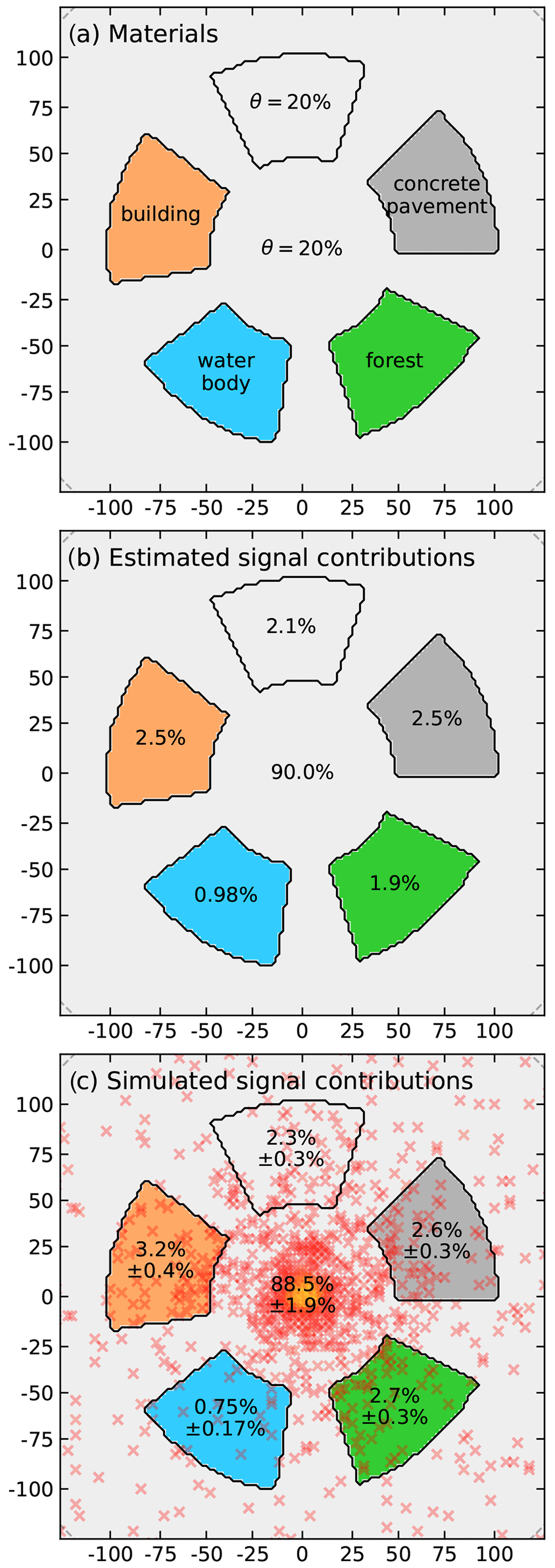
Figure 5(a) Exemplary scenario with different land-use features (see Sect. 3.2), (b) analytically estimated signal contributions based only on the soil moisture, and (c) URANOS-simulated signal contributions including 3D features (house, trees).
Results shown in Fig. 5 indicate an estimated contribution of the reference area of c1≈2.1 % (panel b), which is well matched by the simulation, 2.3±0.3 % (panel c). The building and the concrete pavement exhibit the same dry material composition in the ground and thus lead to similar estimated contributions, %. In contrast, the simulation shows a much higher contribution of the building, 3.2±0.4 %, since it also accounts for the above-ground house material. The same holds for the forest area, %. As expected, the water body shows the lowest contribution, %.
In general, the analytical approach seems to provide good performance throughout different land-use regimes, with minor deviations at the pure-water end of the soil moisture spectrum. Significant limitations of the purely ground-driven approach are evident for above-ground objects, such as forests or buildings. In these cases, however, the method might still be applicable by defining a “soil moisture equivalent” of those land-use types. For example, setting vol % and vol % would lead to a perfect match with the simulations for the forest and the building, respectively. While these values certainly depend on the specific material composition and distance of the actual building or forest, future studies may show whether the contribution of these very special land-use types can be generalized.
3.3 Impact on the N(θ) relationship
The insight that different areas in the footprint have different contributions to the finally detected signal raises the question of whether complex terrain can change the shape of the N(θ) relationship, which was initially derived from homogeneous model conditions. In fact, many authors have reported deviation of their data from the standard N(θ) curve and reacted by empirically deriving site-specific parameterizations to change its shape (Rivera Villarreyes et al., 2011; Lv et al., 2014; Iwema et al., 2015; Heidbüchel et al., 2016; Schattan et al., 2017, 2019). In this section, we suggest that the effect of non-homogeneous signal contributions might help to explain these observations. Following the idea of the areal correction introduced by Schrön et al. (2018a), we aim at generalizing this approach to a correction based on the signal contributions.
The application of such a correction will be explained by the following theoretical example. Consider an area of interest A1∈Ω, for which the soil moisture dynamics are to be measured by a neutron detector. A second area, , which does not respond to soil moisture changes, e.g. a concrete pavement, a building, a water body, a swamp, or rocky terrain, lies within the sensor footprint. This area will generate a constant, invariant stream of neutrons, N(θ2=const.), and thus dampen the total effective neutron measurement as a function of θ1.
In order to correct for the damping effect, we propose to rescale the amplitude of the neutron counts by the signal contribution c1 from area A1, because only this fraction will be able to stimulate neutron dynamics:
where Nref=N(θ2) is a stationary reference offset (i.e. an invariant neutron stream from area A2) around which the amplitude will be stretched in order to make sure that the correction sustains identity for θ1=θ2. If θ2 is not known, the mean observed neutron counts could be a first-order approximation, as has been done in an urban terrain by Schrön et al. (2018a).
The approach is tested in an exemplary scenario with a central area of 20 m radius and variable soil moisture, θ1, surrounded by an area of constant soil moisture of θ2=10 vol % (Fig. 6a). The signal contribution of the inner area varies from 30 % to 41 % depending on θ1, with a mean of c1≈33 % (Eq. 7). Figure 6b shows the simulated effective neutron intensity of the central detector as a function of θ1 (blue points), the standard N(θ) relationship (black line; see also Fig. 1b), and the function Nresc which was rescaled by the factor c1 (Eq. 12) to resemble the damping effect (dashed blue line). The shaded area represents the mentioned range of c1 and demonstrates the robustness of the approach if the signal contribution cannot be determined precisely.
In summary, this application of the signal contribution theory offers an explanation for site-specific parameterizations of the N(θ) relationship, which could be tested with existing and future CRNS data sets.
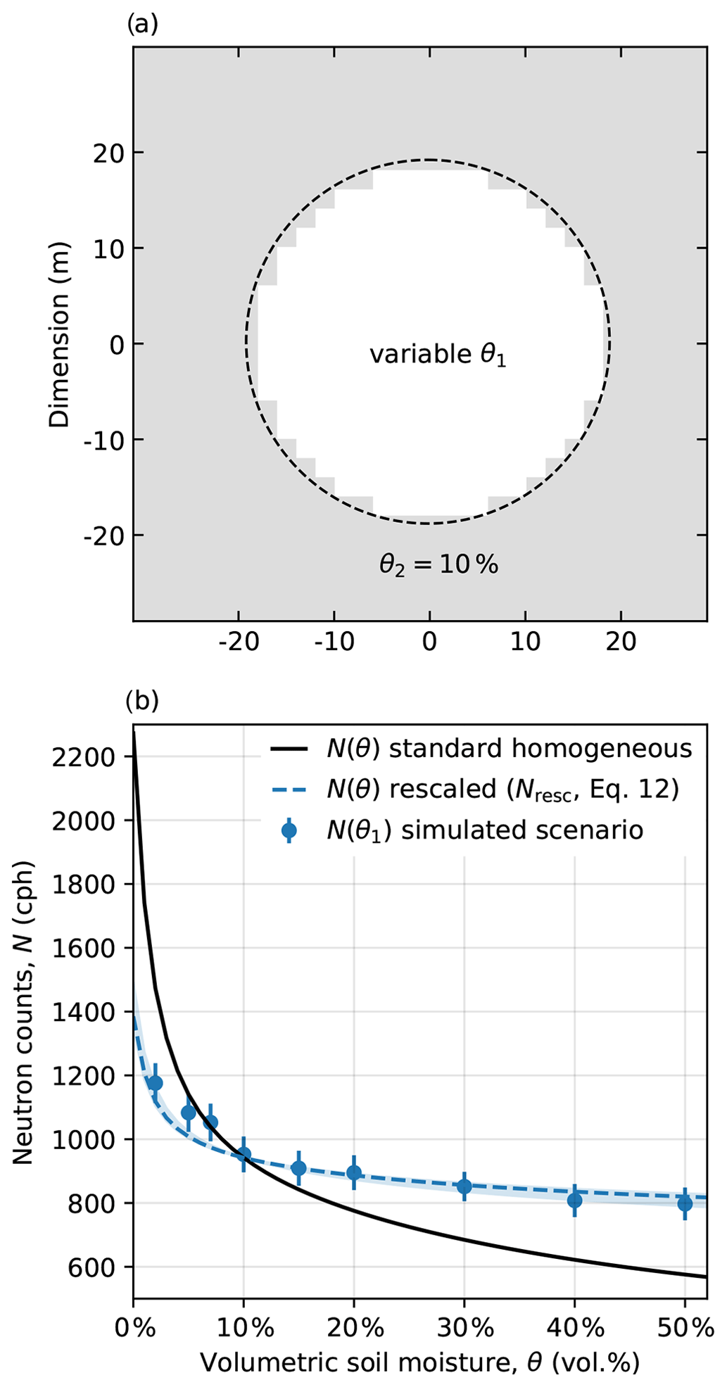
Figure 6Exemplary scenario to demonstrate the impact of signal contributions on the N(θ) relationship. (a) Scenario with variable soil moisture, θ1, in a central area of a 20 m radius, surrounded by constant soil moisture of θ2=10 vol % (e.g. concrete pavement). The signal contribution of the inner area is c1≈33 %. (b) The simulated effective neutron intensity of the central detector as a function of θ1 (blue points) appears damped compared to the standard relationship (black line; see also Fig. 1b). However, the function can be rescaled using c1 and Eq. (12) to resemble the damping effect (dashed blue line). The shaded area represents the range of c1 (30 %–41 %) depending on soil moisture.
3.4 Remote field at a distance
In this section, the signal estimation approach is challenged with a more simplistic scenario, but this time without radial symmetry, in order to represent typical land-use geometries. The investigated domain is split into two half-spaces with different soil moisture, like two agricultural fields neighbouring each other or like partly irrigated land.
In the first exemplary scenario, the soil moisture of the two fields is set to θ1=10 vol % and θ2=30 vol %. According to Eqs. (6)–(7), the dry area contributes c1≈58 % and the wet area c2≈42 % of the total neutron count rate, while the apparent soil moisture average is vol % (Eq. 10). This value is substantially lower than the naive mean, vol %, due to the non-linearity of the θ(N) relationship (Fig. 1b). URANOS simulation results confirm this approach with vol %.
In order to extend the analysis to arbitrary domain splits, we now consider a scenario that consists of two areas split at the distance R from the centre, where A1(x≤R) is the field around the central detector and A2(x>R) is the remote field. The interface between the two fields is a straight line orthogonal to the x axis as illustrated in Fig. 7. The total neutron count rate can be described following Eq. (6):
The weight w in the Cartesian geometry is expressed in radial coordinates to avoid any corner effects, since the nature of neutron transport and detection usually follows radial symmetry. The term represents the length of an arc within the circle area constrained by x>R (see also Fig. 8a). It can be derived from the opening angle of the sector, , where 2α is the same fraction of 2π as is the arc of the total circumference 2π r.
In general, a purely radial geometry, where soil moisture changes in the whole region defined by r>R, would be a more simple scenario to calculate. However, we believe these radial field arrangements to be a rather rarely encountered situation compared to the much more typical straight field geometries. In cases where circular fields and the corresponding soil moisture differences are relevant (e.g. for pivot irrigation, Finkenbiner et al., 2019), the integrand can simply be solved without the term.
In the homogeneous case with soil moisture θ1=θ2, the apparent average soil moisture also equals , and the total neutron count rate results to . If the remote area changes from θ1 to θ2, however, the weighting function of the total domain changes slightly. The influence of this change on is usually marginal for small changes or high distances, but the calculation could be reiterated along updates of if precision matters.
We investigated an example scenario of a remote field at the minimal distance R=207 m and soil moisture distributions of θ1=5 vol % and θ2=10 vol % (Fig. 7a). Equations (13) and (7) describe the influence of the remote field to the detected neutron count rate in the centre. The estimated contribution to the total neutron signal is % (Fig. 7b). This is significant to most CRNS detectors, since typical count rates of 1000 cph imply uncertainties between 0.6 % (daily) and 3.2 % (hourly resolution). Simulation results shown in Fig. 7c precisely confirm this result with 3.0 %. Here, the red crosses depict the locations where detected neutrons had first contact with the soil, indicating the contribution of the corresponding region to the signal.
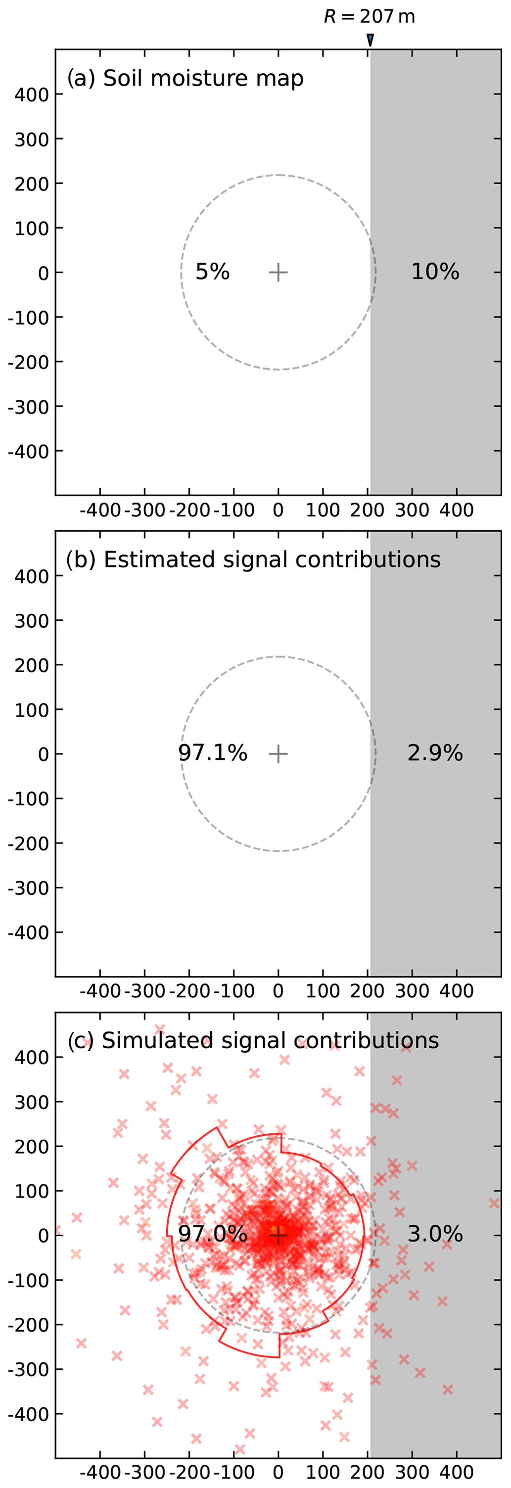
Figure 7Scenario with (a) soil moisture distributed in the main field (θ1, white) and in the remote field (θ2, grey) at the distance of R=207 m; the circle indicates the R86 footprint. (b) Contribution to the detector signal estimated with the analytical method and (c) simulated with URANOS (neutron origins as red crosses, angular footprint shape in 30∘ steps as red line).
The slightly asymmetric distribution of these origins often indicates an amoeba-like shape of the footprint; see also the red line in Fig. 7c. This suggests that the assumption of a symmetric footprint radius, R86, no longer holds (as has also been shown by Köhli et al., 2015; Schattan et al., 2019).
Interesting to note is that the effectively measured soil moisture in this example is vol %. Although the remote field is very close to the outer margins of the radial footprint R86, it still contributes 3 % to the total neutron intensity and thereby increases the CRNS-averaged soil moisture by 0.1 vol %. The dry bias can be explained by the large distance of the wetter field (which is even larger than R at all but one point), as well as by the strong non-linearity of Wr towards lower r (Fig. 1a), and the non-linearity of the θ(N) relationship (Fig. 1b).
In general, an exact understanding of the weighting function Wr(h,θ) plays an essential role in precise estimation of far-field influences. This sensitivity can be illustrated using the approximation (Eq. 2). It is usually less accurate due to the missing dependency on air humidity and soil moisture. Considering an exemplary scenario with θ1=5 vol % and a field at R=57 m distance with θ2=10 vol %, the “actual” signal contribution of the remote field is c2=15.3 %, calculated by URANOS. The accurate theoretical estimation using Wr(h,θ) yields c2=14.7 %, while the simplified approach only yields 11.9 %.
3.5 A practical footprint definition based on field distance and detector sensitivity
This section proposes a more practical definition of the footprint size for rectangular field geometries. The definition will be built upon the answer to the following research question: at what distance are soil moisture changes still visible to the CRNS? Or, more precisely, at what maximum distance R from a distant field should the detector be located such that a change in soil moisture by still has significant contribution ΔN≥σN to the detected neutron signal?
As it has been shown in the previous sections, the intensity distribution around the sensor, Wr(h,θ), weights different regions of the footprint in a highly unequal way. Therefore, a new approach is suggested to interpret the footprint as the distance R, to which a remote change of soil moisture is still visible in the detector signal.
In order to assess this sensitivity, we reject all neutron intensity changes below a certain significance level of the sensor. The relative stochastic precision of a neutron detector, , highly depends on the count rate N (Zreda et al., 2012; Weimar et al., 2020). It is a function of detector volume, its efficiency, atmospheric conditions, soil moisture, and temporal aggregation (see e.g. the concept of N0,base in Schrön et al., 2021).
For average conditions, usual CRNS detectors with an average count rate of N≈1000 cph can achieve a precision of σN=3.2 % h−1 or % d−1. With regard to increasingly improving detectors and to the generally relevant timescales of 6–12 h, we condition our analysis on the σN=1 % uncertainty limit; i.e. we will consider CRNS detectors sensitive to a certain environmental change if the induced relative change of the count rate exceeds 1 %. Note that this definition implicates that the practical footprint R may be different for different detectors, site conditions, and temporal aggregations. Yet, as current commercial stationary systems are limited to N≈5000 cph, this approach can be regarded as relevant to all existing installations.
Following the above concept of the remote fields, changes of remote soil moisture conditions will only be measurable if the difference between the total neutron count rates before, , and after the change, , is larger than the precision limit:
Equations (13) and (14) can be solved for R numerically, while an analytical solution is not straightforward due to the complexity of Wr(h,θ). To facilitate easy application of this approach for scientists and CRNS users, an interactive online tool has been developed and is briefly presented in Appendix A. For the change θ1→θ2 we suggest to use Δθ=10 vol %, which is a good compromise between typical artificial or natural variations of soil moisture that are of interest for hydrologists. The Supplement contains the results for R using more combinations of parameters for h (1–15 g m−3), θ1 (1 vol %–50 vol %), Δθ (±2.5 vol %–20 vol %), and σN (1 %–3 %).
Calculation results of the distance R are shown in Table 1 for a range of soil moisture θ1 from 1 to 50 vol %, where θ2 is always larger by +10 vol %. The measurement precision is investigated for two cases, σN=1 % and 2 %. It is evident that the distance to the field must be much smaller if the detection precision is worse. For example, standard detectors at 2-hourly resolution (σN≈2 %) would be able to reliably detect +10 vol % soil moisture changes of an adjacent field at R=1 m distance, even for extremely wet conditions.
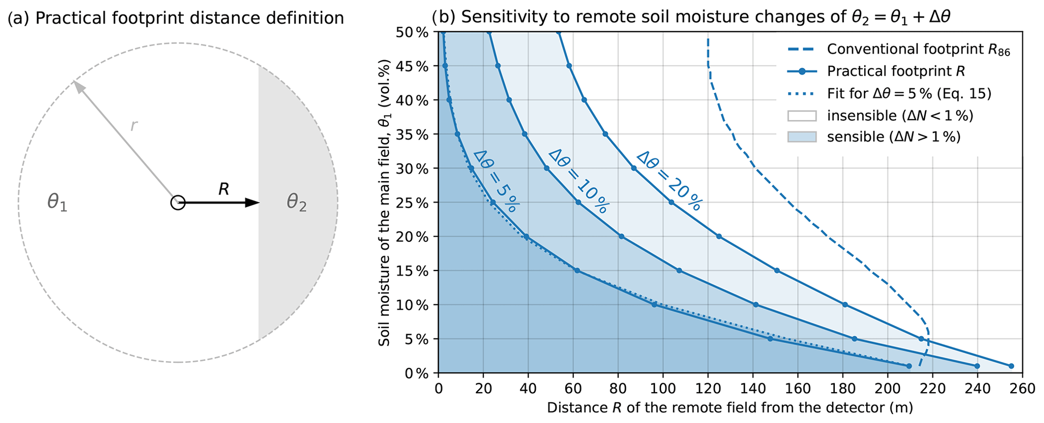
Figure 8(a) Schematic illustration in radial coordinates of the practical footprint definition. It represents the maximal orthogonal distance R to a remote field (grey) such that its change of soil moisture from θ1 to is still sensible by the central detector. (b) Main field soil moisture θ1 over distance R to the remote field for sensor precision σN=1 %, air humidity h=5 g m−3, and three wetting cases Δθ. Assuming a main field soil moisture of 15 vol %, for instance, an increase in remote field soil moisture by +5 vol % is sensible (i.e. ΔN>σN) if the distance to that field is not larger than 60 m. The dotted line is an analytical formulation of R (Eq. 15) as a function of the conventional footprint radius R86 (shown as a dashed line for comparison) and performs well in approximating the simulated values (points).
Table 1Analytical results for the minimal footprint distance R such that soil moisture changes of a remote field ( vol %) in an initially uniform domain (θ2=θ1, h=5 g m−3) become visible by the CRNS (see Fig. 7 for an illustration with R=207 m). Cases consider CRNS measurement precision values of σN=1 % and 2 %; more cases for σN, h, and Δθ are presented in the Sect. S1. Conventional footprints R86 are displayed for comparison; soil moisture is displayed in vol %. The effectively apparent soil moisture is dry-biased due to the non-linearity of θ(N).
Figure 8b shows the calculated ranges for h=5 g m−3, σN=1 %, and three different soil moisture changes of the remote field, vol %. For arid regions between 1 % and 5 % of soil water content, the changes of +5 vol % are visible to the detector at distances above 150 m. In humid climate of up to 25 vol % water content, wetter remote fields beyond 20 m distance will not show significant contribution to the detector. In wetland areas, +5 vol % changes of soil moisture are hardly measurable even if this area covers almost half of the footprint. Higher soil moisture changes of Δθ=10 vol % and 20 vol % (e.g. during irrigation) are much more prominent in the neutron signal and thus allow the remote field to be at a larger distance from the sensor.
The figure also indicates the conventional footprint radius R86 (dashed line) based on Köhli et al. (2015) and Schrön et al. (2017). Under most conditions, R86 is much larger than R, as it accounts for neutron intensity changes in all directions (not only a one-sided remote field), and it has not been restricted to the mentioned accuracy limits and soil moisture changes. The radial footprint definition also fails to explain that extensive irrigation of a remote field in arid regions can be sensible much beyond the conventional footprint radius.
Similar to the wetting of the remote field, Δθ>0, also the case of soil drying, Δθ<0, has been investigated. Due to the non-linearity of N(θ), the neutron production in dry areas is disproportionally higher than the neutron reduction in wet areas. This leads to a strong influence of distant dry fields under otherwise wet conditions, which consequently manifests in longer maximal distances R by factors of 1.5 (under wet) to 2.0 (under dry conditions). For example, in an area with θ=20 vol %, a dry-out by −10 vol % can be detected from a field at up to a 140 m distance, while a wetting of that field by +10 vol % is only detectable from up to an 80 m distance. The corresponding tabulated data are provided in the Supplement.
Using a numerical fit, the new practical footprint distance R can be expressed relative to the conventional footprint radius (solid lines in Fig. 8b):
where θ=θ1 in units of m3 m−3, m3 m−3, and σN=1 %. Practical functions for higher soil moisture changes Δθ and higher measurement uncertainty σN could be determined using the presented calculation procedure or the provided data in the Supplement.
The relative formulation based on R86 already accounts for most dependencies on air pressure, air humidity, and other factors. The equation has been tested for various air humidity conditions, for instance, and indicated good performance (not shown). If the radial footprint radius is not known, an even further simplified approximation for average air humidity h, standard air pressure P, m3 m−3, and σN=1 % would be
While these relationships may be useful to quickly assess the potential influence of distant fields on the sensor signal, we strongly encourage researchers to perform experiments (e.g. strategic irrigation) that could appropriately falsify the presented theory.
This paper presents an analytical approach to determine the contributions of distant areas in the footprint to the detected signal within the framework of cosmic-ray neutron sensing (CRNS). In various examples using splitted fields, heterogeneous soil moisture pattern, or complex land-use types, the calculations have been verified with neutron transport simulations. The results showed that even complex distributions of simulated neutron intensities can indeed be approximated using the new approach, indicating that secondary interactions between individual areas are of minor importance. The approach could be easily adapted to individual site conditions in order to quantify the influence of structures, vegetated land, or irrigated fields in the footprint. The proposed method has the potential to improve sensor positioning, site-specific calibration, and signal interpretation.
Based on this concept, two applications for the CRNS signal interpretation have been investigated. First, we found that knowledge about the signal contribution of the area of interest could help to explain seemingly site-specific shapes of the N(θ) relationship. The area's signal contribution value could be used to rescale the neutron–moisture relationship such that the damping effect of invariant landscape features can be excluded from the signal (Fig. 6). Second, a new footprint definition has been proposed which represents the maximum orthogonal distance to a remote field (Fig. 8a) such that its soil moisture changes are still visible in the measured neutron signal. In the presentation of the results, a typical detector precision of σN=1 % and positive soil moisture changes of vol % to +20 vol % have been chosen, while the approach is adaptable to any combination of parameters. The resulting practical footprint distances for wetting remote fields are 1–90 m (wet climate), 18–180 m (humid), and 100–255 m (arid), showing a strong dependence on the initial soil moisture conditions in the field. In contrast, the dry-out of remote fields (Δθ<0) is usually easier to detect due to the non-linearity of the neutron–water relationship, leading to 1.5–2.0 times larger distances.
To date, the footprint of a CRNS sensor has been interpreted as a regular circle. The presented results show that the assumption of the radial geometry of the footprint is not suitable for very heterogeneous and complexly structured regions. In fact, remote fields extending beyond the minimum tangential distance R<x, by this definition, usually provide less signal contribution than radial fields beyond R86<r. This is why R is usually shorter than R86. However, in some cases, R can be even larger than R86 for very dry regions and strong soil moisture gradients. This already indicates the low explanatory power of the radially symmetric formulation for some situations with rectangular geometries. In these cases, the new Cartesian footprint definition could be more informative.
In situations when sensor placement is not possible in homogeneous environments, it is crucial to realize that the sensor does not inherently provide a simple areal average of the heterogeneous soil moisture patterns in the footprint. In fact, this study showed that parts of the footprint can have a different contribution to the averaged signal depending on their size and distance, while the non-linear nature of N(θ) will often underestimate the average soil moisture of two equally sized areas, as was also shown by Franz et al. (2013).
To learn more about the way how a CRNS station responds to its environment, we recommend to apply the presented method by forward modelling various soil moisture scenarios. This way, one could learn about the potential signal contributions from different landscape compartments and the implications for data uncertainty and hydrological process identification. The tool can also be used to quantify the challenges in signal interpretation already in the preparation phase prior to measurement campaigns. This could be an important aid with regard to the optimization of sensor placements.
The method could also support hydrological modelling or geostatistical inverse models, where forward operators are required to predict the neutron intensity in a computationally efficient way (Shuttleworth et al., 2013; Franz et al., 2015; Heistermann et al., 2021). Here, the analytical calculations could facilitate spatial neutron modelling even in complex environments without computationally expensive Monte Carlo transport simulations. In addition to the first evidence provided by Schrön et al. (2018a), we recommend future studies to evaluate this approach against dedicated simulations and real field data.
To test and apply the presented method, researchers and users may employ an easy-to-use online tool, available from https://github.com/mschroen/crns-signalcontrib. We developed an interactive Jupyter Notebook which is hosted on GitHub and can be run using Binder, a service that allows everyone to run Python code from the browser without installations or prior knowledge. All necessary numerical calculations related to the footprint distance and sensitivity concept are already implemented in the notebook such that calculations of the footprint distance, signal contributions, and significance tests can be performed for user-defined soil moisture conditions (Fig. A1).
Figure A1Showcase of an interactive Jupyter Notebook hosted by Binder. The tool allows us to calculate the footprint distance, contributions, and significance of certain soil moisture conditions. It is accessible from the browser and does not require prior installation or programming knowledge.
The supplement related to this article is available online at: https://doi.org/10.5194/hess-27-723-2023-supplement.
MS developed the theory of signal contributions. MS, MK, and SZ developed the concept of an alternative footprint definition. MS performed the calculations and analysis. MS wrote the first version of the manuscript. MS, MK, and SZ edited and contributed to the substantial improvement of the manuscript.
Markus Köhli holds a CEO position at StyX Neutronica GmbH, Germany.
Publisher’s note: Copernicus Publications remains neutral with regard to jurisdictional claims in published maps and institutional affiliations.
The authors thank Jannis Weimar (Heidelberg University), Maik Heistermann (University of Potsdam), and Daniel Rasche (GFZ Potsdam) for fruitful discussions.
This research has been supported by the Deutsche Forschungsgemeinschaft (grant no. 357874777; research unit FOR 2694, Cosmic Sense) and the Bundesministerium für Bildung und Forschung (grant no. 02WIL1522; German–Israeli Cooperation in Water Technology Research).
The article processing charges for this open-access publication were covered by the Helmholtz Centre for Environmental Research – UFZ.
This paper was edited by Nunzio Romano and reviewed by four anonymous referees.
Andreasen, M., Jensen, K. H., Desilets, D., Zreda, M., Bogena, H. R., and Looms, M. C.: Cosmic-ray neutron transport at a forest field site: the sensitivity to various environmental conditions with focus on biomass and canopy interception, Hydrol. Earth Syst. Sci., 21, 1875–1894, https://doi.org/10.5194/hess-21-1875-2017, 2017a. a
Andreasen, M., Jensen, K. H., Desilets, D., Franz, T. E., Zreda, M., Bogena, H. R., and Looms, M. C.: Status and Perspectives on the Cosmic-Ray Neutron Method for Soil Moisture Estimation and Other Environmental Science Applications, Vadose Zone J., 16, vzj2017.04.0086, https://doi.org/10.2136/vzj2017.04.0086, 2017b. a
Baroni, G. and Oswald, S. E.: A scaling approach for the assessment of biomass changes and rainfall interception using cosmic-ray neutron sensing, J. Hydrol., 525, 264–276, https://doi.org/10.1016/j.jhydrol.2015.03.053, 2015. a
Bogena, H. R., Huisman, J. A., Baatz, R., Hendricks-Franssen, H.-J., and Vereecken, H.: Accuracy of the cosmic-ray soil water content probe in humid forest ecosystems: The worst case scenario, Water Resour. Res., 49, 5778–5791, https://doi.org/10.1002/wrcr.20463, 2013. a
Coopersmith, E. J., Cosh, M. H., and Daughtry, C. S.: Field-scale moisture estimates using COSMOS sensors: A validation study with temporary networks and Leaf-Area-Indices, J. Hydrol., 519, 637–643, https://doi.org/10.1016/j.jhydrol.2014.07.060, 2014. a
Desilets, D. and Zreda, M.: Footprint diameter for a cosmic‐ray soil moisture probe: Theory and Monte Carlo simulations, Water Resour. Res., 49, 3566–3575, https://doi.org/10.1002/wrcr.20187, 2013. a, b
Desilets, D., Zreda, M., and Ferré, T. P. A.: Nature's neutron probe: Land surface hydrology at an elusive scale with cosmic rays, Water Resour. Res., 46, W11505, https://doi.org/10.1029/2009WR008726, 2010. a, b
Fersch, B., Francke, T., Heistermann, M., Schrön, M., Döpper, V., Jakobi, J., Baroni, G., Blume, T., Bogena, H., Budach, C., Gränzig, T., Förster, M., Güntner, A., Hendricks Franssen, H.-J., Kasner, M., Köhli, M., Kleinschmit, B., Kunstmann, H., Patil, A., Rasche, D., Scheiffele, L., Schmidt, U., Szulc-Seyfried, S., Weimar, J., Zacharias, S., Zreda, M., Heber, B., Kiese, R., Mares, V., Mollenhauer, H., Völksch, I., and Oswald, S.: A dense network of cosmic-ray neutron sensors for soil moisture observation in a highly instrumented pre-Alpine headwater catchment in Germany, Earth Syst. Sci. Data, 12, 2289–2309, https://doi.org/10.5194/essd-12-2289-2020, 2020. a
Finkenbiner, C. E., Franz, T. E., Gibson, J., Heeren, D. M., and Luck, J.: Integration of hydrogeophysical datasets and empirical orthogonal functions for improved irrigation water management, Precis. Agric., 20, 78–100, 2019. a
Francke, T., Heistermann, M., Köhli, M., Budach, C., Schrön, M., and Oswald, S. E.: Assessing the feasibility of a directional cosmic-ray neutron sensing sensor for estimating soil moisture, Geosci. Instrum. Method. Data Syst., 11, 75–92, https://doi.org/10.5194/gi-11-75-2022, 2022. a
Franz, T. E., Zreda, M., Ferré, T. P. A., and Rosolem, R.: An assessment of the effect of horizontal soil moisture heterogeneity on the area-average measurement of cosmic-ray neutrons, Water Resour. Res., 49, 6450–6458, https://doi.org/10.1002/wrcr.20530, 2013. a, b, c
Franz, T. E., Wang, T., Avery, W., Finkenbiner, C., and Brocca, L.: Combined analysis of soil moisture measurements from roving and fixed cosmic ray neutron probes for multiscale real-time monitoring, Geophys. Res. Lett., 42, 3389–3396, https://doi.org/10.1002/2015GL063963, 2015. a
Franz, T. E., Wahbi, A., Vreugdenhil, M., Weltin, G., Heng, L., Oismueller, M., Strauss, P., Dercon, G., and Desilets, D.: Using Cosmic-Ray Neutron Probes to Monitor Landscape Scale Soil Water Content in Mixed Land Use Agricultural Systems, Appl. Environ. Soil Sci., 2016, 1–11, https://doi.org/10.1155/2016/4323742, 2016. a, b
Heidbüchel, I., Güntner, A., and Blume, T.: Use of cosmic-ray neutron sensors for soil moisture monitoring in forests, Hydrol. Earth Syst. Sci., 20, 1269–1288, https://doi.org/10.5194/hess-20-1269-2016, 2016. a, b
Heistermann, M., Francke, T., Schrön, M., and Oswald, S. E.: Spatio-temporal soil moisture retrieval at the catchment scale using a dense network of cosmic-ray neutron sensors, Hydrol. Earth Syst. Sci., 25, 4807–4824, https://doi.org/10.5194/hess-25-4807-2021, 2021. a, b
Iwema, J., Rosolem, R., Baatz, R., Wagener, T., and Bogena, H. R.: Investigating temporal field sampling strategies for site-specific calibration of three soil moisture–neutron intensity parameterisation methods, Hydrol. Earth Syst. Sci., 19, 3203–3216, https://doi.org/10.5194/hess-19-3203-2015, 2015. a, b, c, d
Jakobi, J., Huisman, J. A., Köhli, M., Rasche, D., Vereecken, H., and Bogena, H. R.: The Footprint Characteristics of Cosmic Ray Thermal Neutrons, Geophys. Res. Lett., 48, e2021GL094281, https://doi.org/10.1029/2021gl094281, 2021. a
Kasner, M., Zacharias, S., and Schrön, M.: On soil bulk density and its influence to soil moisture estimation with cosmic-ray neutrons, Hydrol. Earth Syst. Sci. Discuss. [preprint], https://doi.org/10.5194/hess-2022-123, in review, 2022. a
Köhli, M., Schrön, M., Zreda, M., Schmidt, U., Dietrich, P., and Zacharias, S.: Footprint characteristics revised for field-scale soil moisture monitoring with cosmic-ray neutrons, Water Resour. Res., 51, 5772–5790, https://doi.org/10.1002/2015WR017169, 2015. a, b, c, d, e, f, g, h, i, j
Köhli, M., Schrön, M., and Schmidt, U.: Response functions for detectors in cosmic ray neutron sensing, Nuclear Instruments and Methods in Physics Research Section A: Accelerators, Spectrometers, Detectors and Associated Equipment, 902, 184–189, https://doi.org/10.1016/j.nima.2018.06.052, 2018. a
Köhli, M., Weimar, J., Schrön, M., and Schmidt, U.: Moisture and humidity dependence of the above-ground cosmic-ray neutron intensity, Front. Water, 2, 66, https://doi.org/10.3389/frwa.2020.544847, 2021. a, b, c
Köhli, M., Schrön, M., Zacharias, S., and Schmidt, U.: URANOS v1.0 – the Ultra Rapid Adaptable Neutron-Only Simulation for Environmental Research, Geosci. Model Dev., 16, 449–477, https://doi.org/10.5194/gmd-16-449-2023, 2023. a, b
Li, D., Schrön, M., Köhli, M., Bogena, H. R., Weimar, J., Bello, M. A. J., Han, X., Gimeno, M. A. M., Zacharias, S., Vereecken, H., and Hendricks-Franssen, H.: Can Drip Irrigation be Scheduled with Cosmic‐Ray Neutron Sensing?, Vadose Zone J., 18, 190053, https://doi.org/10.2136/vzj2019.05.0053, 2019. a, b
Lv, L., Franz, T. E., Robinson, D. A., and Jones, S. B.: Measured and Modeled Soil Moisture Compared with Cosmic‐Ray Neutron Probe Estimates in a Mixed Forest, Vadose Zone J., 13, 1–13, https://doi.org/10.2136/vzj2014.06.0077, 2014. a, b, c, d
Ragab, R., Evans, J. G., Battilani, A., and Solimando, D.: The Cosmic‐ray Soil Moisture Observation System (Cosmos) for Estimating the Crop Water Requirement: New Approach, Irrig. Drain., 66, 456–468, https://doi.org/10.1002/ird.2152, 2017. a
Rasche, D., Köhli, M., Schrön, M., Blume, T., and Güntner, A.: Towards disentangling heterogeneous soil moisture patterns in cosmic-ray neutron sensor footprints, Hydrol. Earth Syst. Sci., 25, 6547–6566, https://doi.org/10.5194/hess-25-6547-2021, 2021. a
Rivera Villarreyes, C. A., Baroni, G., and Oswald, S. E.: Integral quantification of seasonal soil moisture changes in farmland by cosmic-ray neutrons, Hydrol. Earth Syst. Sci., 15, 3843–3859, https://doi.org/10.5194/hess-15-3843-2011, 2011. a, b
Schattan, P., Baroni, G., Oswald, S. E., Schöber, J., Fey, C., Kormann, C., Huttenlau, M., and Achleitner, S.: Continuous monitoring of snowpack dynamics in alpine terrain by aboveground neutron sensing, Water Resour. Res., 53, 3615–3634, https://doi.org/10.1002/2016WR020234, 2017. a, b, c
Schattan, P., Köhli, M., Schrön, M., Baroni, G., and Oswald, S. E.: Sensing Area-Average Snow Water Equivalent with Cosmic-Ray Neutrons: The Influence of Fractional Snow Cover, Water Resour. Res., 55, 10796–10812, https://doi.org/10.1029/2019WR025647, 2019. a, b, c, d, e, f
Scheiffele, L. M., Baroni, G., Franz, T. E., Jakobi, J., and Oswald, S. E.: A profile shape correction to reduce the vertical sensitivity of cosmic‐ray neutron sensing of soil moisture, Vadose Zone J., 19, e20083, https://doi.org/10.1002/vzj2.20083, 2020. a
Schrön, M., Zacharias, S., Köhli, M., Weimar, J., and Dietrich, P.: Monitoring Environmental Water with Ground Albedo Neutrons from Cosmic Rays, in: The 34th International Cosmic Ray Conference, vol. 236, p. 231, SISSA Medialab, https://doi.org/10.22323/1.236.0231, 2016. a
Schrön, M., Köhli, M., Scheiffele, L., Iwema, J., Bogena, H. R., Lv, L., Martini, E., Baroni, G., Rosolem, R., Weimar, J., Mai, J., Cuntz, M., Rebmann, C., Oswald, S. E., Dietrich, P., Schmidt, U., and Zacharias, S.: Improving calibration and validation of cosmic-ray neutron sensors in the light of spatial sensitivity, Hydrol. Earth Syst. Sci., 21, 5009–5030, https://doi.org/10.5194/hess-21-5009-2017, 2017. a, b, c, d, e, f, g, h, i, j, k
Schrön, M., Zacharias, S., Womack, G., Köhli, M., Desilets, D., Oswald, S. E., Bumberger, J., Mollenhauer, H., Kögler, S., Remmler, P., Kasner, M., Denk, A., and Dietrich, P.: Intercomparison of cosmic-ray neutron sensors and water balance monitoring in an urban environment, Geosci. Instrum. Method. Data Syst., 7, 83–99, https://doi.org/10.5194/gi-7-83-2018, 2018a. a, b, c, d, e, f, g, h, i, j
Schrön, M., Rosolem, R., Köhli, M., Piussi, L., Schröter, I., Iwema, J., Kögler, S., Oswald, S. E., Wollschläger, U., Samaniego, L., Dietrich, P., and Zacharias, S.: Cosmic-ray Neutron Rover Surveys of Field Soil Moisture and the Influence of Roads, Water Resour. Res., 54, 6441–6459, https://doi.org/10.1029/2017WR021719, 2018b. a
Schrön, M., Oswald, S. E., Zacharias, S., Kasner, M., Dietrich, P., and Attinger, S.: Neutrons on Rails: Transregional Monitoring of Soil Moisture and Snow Water Equivalent, Geophys. Res. Lett., 48, e2021GL093924, https://doi.org/10.1029/2021GL093924, 2021. a
Schrön, M.: CRNS Signal Contributions (1.01), Zenodo [code], https://doi.org/10.5281/zenodo.7607054, 2023. a
Shuttleworth, J., Rosolem, R., Zreda, M., and Franz, T.: The COsmic-ray Soil Moisture Interaction Code (COSMIC) for use in data assimilation, Hydrol. Earth Syst. Sci., 17, 3205–3217, https://doi.org/10.5194/hess-17-3205-2013, 2013. a
Tian, J. and Song, S.: Application of Cosmic-Ray Neutron Sensing to Monitor Soil Water Content in Agroecosystem in North China Plain, in: IGARSS 2019, IIEEE T. Geosci. Remote, 2019, 7053–7056, https://doi.org/10.1109/IGARSS.2019.8900107, 2019. a
Weimar, J., Köhli, M., Budach, C., and Schmidt, U.: Large-Scale Boron-Lined Neutron Detection Systems as a 3He Alternative for Cosmic Ray Neutron Sensing, Front. Water, 2, 16, https://doi.org/10.3389/frwa.2020.00016, 2020. a
Wollschläger, U., Attinger, S., Borchardt, D., Brauns, M., Cuntz, M., Dietrich, P., Fleckenstein, J. H., Friese, K., Friesen, J., Harpke, A., et al.: The Bode hydrological observatory: a platform for integrated, interdisciplinary hydro-ecological research within the TERENO Harz/Central German Lowland Observatory, Environ. Earth Sci., 76, 1–25, https://doi.org/10.1007/s12665-016-6327-5, 2017. a
Zreda, M., Desilets, D., Ferré, T. P. A., and Scott, R. L.: Measuring soil moisture content non-invasively at intermediate spatial scale using cosmic-ray neutrons, Geophys. Res. Lett., 35, L21402, https://doi.org/10.1029/2008GL035655, 2008. a
Zreda, M., Shuttleworth, W. J., Zeng, X., Zweck, C., Desilets, D., Franz, T., and Rosolem, R.: COSMOS: the COsmic-ray Soil Moisture Observing System, Hydrol. Earth Syst. Sci., 16, 4079–4099, https://doi.org/10.5194/hess-16-4079-2012, 2012. a
what is the influence of a distant area or patches of different land use on the measurement signal?or
is the detector sensitive enough to detect a change of soil moisture (e.g. due to irrigation) in a remote field at a certain distance?The concept may support signal interpretation and sensor calibration, particularly in heterogeneous terrain.