Prediction of absolute unsaturated hydraulic conductivity – comparison of four different capillary bundle models

To model water, solute, and energy transport in porous media, it is essential to have accurate information about the soil hydraulic properties (SHPs), i.e., the water retention curve (WRC) and the soil hydraulic conductivity curve (HCC). It is important to have reliable data to parameterize these models, but equally critical is the selection of appropriate SHP models. While various expressions for the WRC are frequently compared, the capillary conductivity model proposed by Mualem (1976a) is widely used but rarely compared to alternatives. The objective of this study was to compare four different capillary bundle models in terms of their ability to accurately predict the HCC without scaling the conductivity function by a measured conductivity value. The four capillary bundle models include two simple models proposed by Burdine (1953) and Alexander and Skaggs (1986), which assume a bundle of parallel capillaries with tortuous flow paths, and two more sophisticated models based on statistical cut-and-random-rejoin approaches, namely those proposed by Childs and Collis-George (1950) and the aforementioned model of Mualem (1976a). To examine how the choice of the WRC parameterization affects the adequacy of different capillary bundle models, we utilized four different capillary saturation models in combination with each of the conductivity prediction models, resulting in 16 SHP model schemes. All schemes were calibrated using 12 carefully selected data sets that provided water retention and hydraulic conductivity data over a wide saturation range. Subsequently, the calibrated models were tested and rated by their ability to predict the hydraulic conductivity of 23 independent data sets of soils with varying textures. The statistical cut-and-random-rejoin models, particularly the Mualem (1976a) model, outperformed the simpler capillary bundle models in terms of predictive accuracy. This was independent of the specific WRC model used. Our findings suggest that the widespread use of the Mualem model is justified.

1 Introduction

Representing the soil hydraulic properties in functional form is useful for simulation of water, energy, and solute transport in the vadose zone. The most established models for the water retention curve (WRC; e.g., van Genuchten, 1980; Kosugi, 1996) and the soil hydraulic conductivity curve (HCC; e.g., Burdine, 1953; Mualem, 1976a) account for water storage and flow in capillaries but neglect water flow and adsorption in films and corners. The latter effects become, however, dominant if the soils get dry. Therefore, more recent models extend these soil hydraulic property (SHP) models (e.g., Tuller and Or, 2001; Peters and Durner, 2008; Lebeau and Konrad, 2010; Zhang, 2011; Peters, 2013; Weber et al., 2019; de Rooij et al., 2021; de Rooij, 2022) to account for these processes. Over the last 10 years, a variety of SHP models have been proposed (see, e.g., Li et al., 2023, and references therein). In the very dry range, vapor flow becomes the dominant transport process. Under isothermal conditions, diffusion of water vapor can be included by an equivalent hydraulic conductivity (Peters, 2013; Iden et al., 2021a, b).

The current models used to predict the HCC, which include both capillary and non-capillary components, do not predict the absolute hydraulic conductivity, K(h), but require scaling of a relative conductivity function, K_r(h), using measured data. Indeed, both the capillary conductivity and the film and corner conductivity must be scaled in some of these models (Peters, 2013). This approach is unsatisfactory as data in the relevant moisture range may be missing (particularly in the dry range) or unreliable (if saturated conductivity is dominated by soil structure), leading to considerable uncertainties in the HCC. To overcome these shortcomings, Peters et al. (2021) proposed a simple yet physically based prediction scheme for the absolute non-capillary conductivity by combining the physically based models for film conductivity proposed by Lebeau and Konrad (2010) and Tokunaga (2009) with the empirical Peters–Durner–Iden (PDI) model developed by Peters (2013, 2014) and Iden and Durner (2014). In a recent study, Peters et al. (2023) extended the HCC prediction from the WRC to the absolute capillary conductivity component using the Mualem (1976a) capillary bundle model. This allows for a conductivity prediction that covers the entire moisture range from near saturation to oven dryness and overcomes the limitations associated with missing or unreliable conductivity data in the relevant moisture range.

A multitude of models has been proposed to describe capillary conductivity. In this work, we focus on the models that derive the pore-size distribution from the capillary water retention function and use the law of Hagen–Poiseuille and some assumptions about connectivity and tortuosity to predict the hydraulic conductivity, the so-called capillary bundle models. We restrict the analysis to the prominent models of Childs and Collis-George (1950), Burdine (1953), Mualem (1976a), and Alexander and Skaggs (1986). As pointed out by Peters et al. (2023), these models are traditionally used to predict the relative conductivity (i.e., the shape of the K(h) relationship) from the WRC and scale it with a measured matching point, most often the measured saturated conductivity (K_s). The models of Burdine (1953) and Alexander and Skaggs (1986) assume that the relative conductivity is derived from a simple bundle of continuous tortuous capillaries. To achieve a simple mathematical expression, Alexander and Skaggs (1986) assumed that the tortuosity depends on capillary saturation and pore radius.

Childs and Collis-George (1950) (CCG) proposed a more sophisticated statistical cut-and-random-rejoin model. This model was later enhanced by Mualem (1976a) through the incorporation of a correlation between pore length and pore diameter in the rejoined pore connections. Comprehensive overviews of the different model types can be found in Mualem and Dagan (1978), Mualem (1986), and Assouline and Or (2013). Although these different models are mentioned in numerous publications, most studies only use Mualem's (1976a) model.

Several comparisons of capillary bundle models have been published. Jackson et al. (1965) compared four models, which are all variations and modifications of the original CCG model, and either predicted the absolute hydraulic conductivity or used one matching factor to scale K_r(h). In their work, the predictions overestimated the conductivities drastically, and the CCG version of Millington and Quirk (1961) with a matching factor gave the best results. Jackson (1972) compared the CCG model versions of Millington and Quirk (1961) and Marshall (1958), which differ in the way tortuosity and pore connectivity are accounted for, by predicting K_r(h) and scaling it with the measured K_s as a matching factor. He found that the models either over- or underestimate K(h) and suggested an intermediate value for the tortuosity and pore connectivity term. Van Genuchten and Nielsen (1985) compared the Mualem (1976a) and Burdine (1953) models in terms of predicting K_r(h) and found the Mualem (1976a) model to perform better. Nimmo and Akstin (1988) compared the models of CCG, Purcell (1949) adapted by Gates and Lietz (1950), Burdine (1953), and Mualem and used one measured unsaturated conductivity as a matching factor. They found, by visual inspection, that the model of Mualem outperformed the other models. Kosugi (1999) compared the Burdine and Mualem models to predict K_r(h) with his generalized version of the Mualem and Dagan (1978) model, which was first fitted to the data to obtain the general parameter values. Not surprisingly, his version outperformed the predictive models. Moreover, the Mualem model performed better than the Burdine model. Hoffmann-Riem et al. (1999) also fitted a general version of the Mualem and Dagan (1978) model to data and compared it with the models of Mualem and Burdine. They concluded that a fit of the models to data should be conducted to obtain a good description. Finally, Madi et al. (2018) compared the capillary bundle models of Burdine (1953), Mualem (1976a), and Alexander and Skaggs (1986) in terms of their applicability in predicting K_r(h). They found that the Alexander and Skaggs model strongly overestimated K(h) for most soils, whereas the performances of the Burdine and Mualem models were superior. None of these studies considered non-capillary conductivity. Moreover, besides the comparison of Jackson et al. (1965), none of the studies conducted a prediction of K(h) without adjusting conductivity parameters.

This study aims to compare capillary bundle models, including Childs and Collis-George (1950), Burdine (1953), Mualem (1976a), and Alexander and Skaggs (1986), regarding their predictive performance for K(h) within the PDI model framework outlined by Peters et al. (2023). To assess the impact of different WRC parameterizations on model performance, we combined four alternative unimodal capillary saturation models with the four conductivity prediction models, resulting in 16 SHP model combinations. Calibration was conducted using 12 data sets providing sufficient information on the WRC and HCC, followed by performance testing on 23 independent data sets representing different soil textures.

2 Theory

All capillary bundle models use a mathematical formulation of the capillary water retention function to express the effective pore-size distribution of a porous medium. We refer to Mualem and Dagan (1978), Mualem (1986), or Peters et al. (2023) for a thorough discussion and mathematical derivation of the most popular capillary bundle models. In this study, we use the Peters–Durner–Iden (PDI) model system (Peters, 2013, 2014; Iden and Durner, 2014) to describe the WRC and HCC in the complete moisture range because it accounts for capillary and non-capillary liquid storage and conductivity as well as vapor conductivity in a simple form and has proven its ability to describe SHP data well. A full description of the PDI model system is given in Appendix A1. In the following, we only briefly review the capillary bundle model formulations used in this study.

2.1 Tortuosity coefficient in capillary bundle models

A key role in all capillary bundle models is played by the so-called tortuosity–connectivity correction, which differs between the various models proposed. It accounts in a lumped manner for all effects that distinguish a porous medium from a bundle of parallel tubes. The term tortuosity itself describes the effect that the path length for single parcels of water, l_p, is longer than the direct projection distance l through the soil. Compared to water flow in straight capillaries, this leads to a reduction in the local conductivity caused by (i) a longer local flow path and (ii) a locally smaller hydraulic gradient (Bear, 1972). The reduction of the effective hydraulic conductivity is expressed by a tortuosity coefficient τ[-]:

$$\begin{array}{}\text{(1)}& \mathit{\tau }={\left({\displaystyle \frac{l}{l_{\mathrm{p}}}}\right)}^{\mathrm{2}}.\end{array}$$

Note that τ is not a constant but a function of water content, since path length increases with decreasing water content. Furthermore, τ≠1 at full water saturation because the flow path is always tortuous.

2.2 Relative capillary hydraulic conductivity prediction by capillary bundle models

Capillary bundle models are typically used to predict the relative capillary conductivity, K_rc(h) [L T⁻¹], and need to be scaled by a scaling parameter, usually the saturated capillary conductivity, K_sc [L T⁻¹], leading to

$$\begin{array}{}\text{(2)}& K_{\mathrm{c}}\left(h\right)=K_{\mathrm{sc}}{K}_{\mathrm{rc}}\left(h\right),\end{array}$$

where K_c [L T⁻¹] is the absolute capillary conductivity. Note that in the original works of Burdine (1953), Childs and Collis-George (1950), Mualem (1976a), and Alexander and Skaggs (1986), K_sc is identical to the total saturated conductivity K_s [L T⁻¹], whereas in the PDI scheme, K_s is given by the sum of saturated capillary and non-capillary conductivities (see Appendix A1).

Burdine model (Bur)

Burdine (1953) suggested that the relative conductivity of porous media is described simply by the conductivity of a bundle of parallel tortuous capillaries of different size, where the tortuosity is inversely related to the capillary saturation, leading to

$$\begin{array}{}\text{(3)}& K_{\mathrm{rc}}=S_{\mathrm{c}}^{\mathrm{2}}{\displaystyle \frac{{\int }_{\mathrm{0}}^{S_{\mathrm{c}}}{h}^{-\mathrm{2}}\mathrm{d}{\stackrel{\mathrm{̃}}{S}}_{\mathrm{c}}}{{\int }_{\mathrm{0}}^{\mathrm{1}}{h}^{-\mathrm{2}}d{\stackrel{\mathrm{̃}}{S}}_{\mathrm{c}}}},\end{array}$$

where ${\stackrel{\mathrm{̃}}{S}}_{\mathrm{c}}$ is the dummy variable of integration. The expression $S_{\mathrm{c}}^{\mathrm{2}}$ describes the dependence of the tortuosity correction on saturation S_c [-] ($\mathrm{0}<S_{\mathrm{c}}<\mathrm{1})$.

Alexander and Skaggs (AS)

Alexander and Skaggs (1986) used a similar expression as Burdine (1953) but assumed that the tortuosity depends on the saturation and the pore radius by $l_{\mathrm{p}}/l=C\sqrt{r/S_{\mathrm{c}}}$, where C [L${}^{-\mathrm{1}/\mathrm{2}}$] is a constant, which was not further specified, yielding

$$\begin{array}{}\text{(4)}& K_{\mathrm{rc}}=S_{\mathrm{c}}{\displaystyle \frac{{\int }_{\mathrm{0}}^{S_{\mathrm{c}}}{h}^{-\mathrm{1}}\mathrm{d}{\stackrel{\mathrm{̃}}{S}}_{\mathrm{c}}}{{\int }_{\mathrm{0}}^{\mathrm{1}}{h}^{-\mathrm{1}}\mathrm{d}{\stackrel{\mathrm{̃}}{S}}_{\mathrm{c}}}}.\end{array}$$

Note that the tortuosity correction is not only given by S_c but is based on the assumption that the tortuosity depends on both saturation and pore radius.

Table 1 Physical constants at 20 ^∘C used in this study.

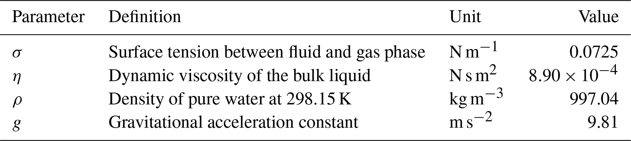
Table 2 Summary of the four prediction models for capillary hydraulic conductivity.

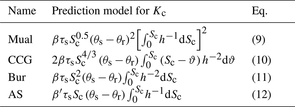
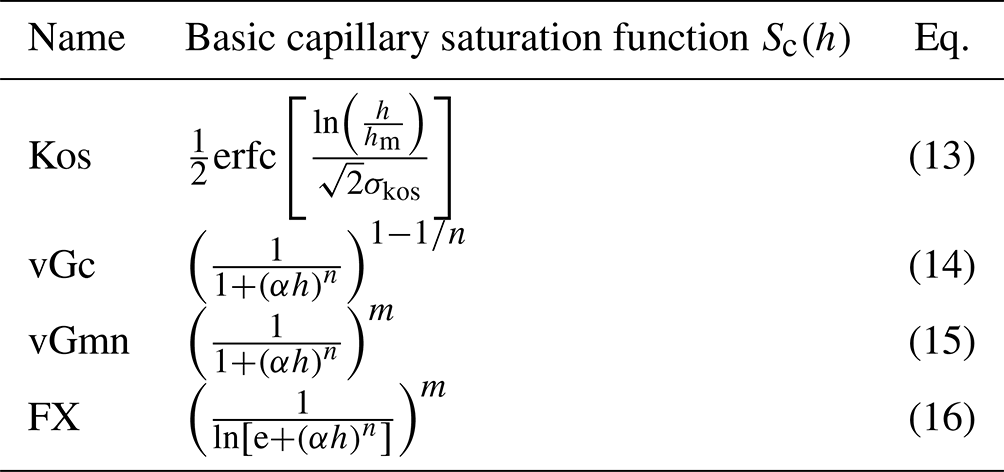
Table 3 Summary of the four capillary saturation functions. The parameters α, n, m, σ_kos, and h_m are shape parameters, and e is the Euler number. These functions are scaled to the value range between 0 and 1 within the PDI scheme by Eq. (A2).

Childs and Collis-George (CGG)

Childs and Collis-George (1950) developed a statistical cut-and-random-rejoin-model, which was further modified by Millington and Quirk (1961) and Kunze et al. (1968) and can be expressed in a general integral form by (Mualem, 1976a)

$$\begin{array}{}\text{(5)}& K_{\mathrm{rc}}=S_{\mathrm{c}}^{\mathit{\lambda }}{\displaystyle \frac{{\int }_{\mathrm{0}}^{S_{\mathrm{c}}}(S_{\mathrm{c}}-\mathit{\vartheta })h^{-\mathrm{2}}\mathrm{d}\mathit{\vartheta }}{{\int }_{\mathrm{0}}^{\mathrm{1}}(\mathrm{1}-\mathit{\vartheta })h^{-\mathrm{2}}\mathrm{d}\mathit{\vartheta }}},\end{array}$$

where ϑ is a variable of integration, which represents the capillary saturation as a function of h between the boundary limits, i.e., 0 and S_c (Mualem and Dagan, 1978). The tortuosity parameter λ [-] is either 1 (Kunze et al., 1968) or $\mathrm{4}/\mathrm{3}$ (Millington and Quirk, 1961).

Mualem (Mual)

Mualem (1976a) used the general approach of CCG and assumed that the length of a pore is directly proportional to its radius, which leads to

$$\begin{array}{}\text{(6)}& K_{\mathrm{rc}}=S_{\mathrm{c}}^{\mathit{\lambda }}{\left[{\displaystyle \frac{{\int }_{\mathrm{0}}^{S_{\mathrm{c}}}{h}^{-\mathrm{1}}\mathrm{d}{\stackrel{\mathrm{̃}}{S}}_{\mathrm{c}}}{{\int }_{\mathrm{0}}^{\mathrm{1}}{h}^{-\mathrm{1}}\mathrm{d}{\stackrel{\mathrm{̃}}{S}}_{\mathrm{c}}}}\right]}^{\mathrm{2}}.\end{array}$$

Applying his model to a variety of data, Mualem found empirically that λ≈0.5.

We may classify these four models into two groups, (i) relatively simple capillary bundle models (Bur, AS), which assume a bundle of parallel capillaries with tortuous flow paths, and (ii) two more sophisticated statistical cut-and-random-rejoin-models (CCG, Mual). Note that the tortuosity correction $S_{\mathrm{c}}^{\mathit{\lambda }}$ in these models becomes unity at saturation because it only describes the relative tortuosity reduction in drying soils.

2.3 Absolute capillary hydraulic conductivity prediction

Peters et al. (2023) (in the remainder “P23”) reformulated the capillary bundle model of Mualem (1976a) to predict absolute capillary conductivity. In a first step, they expressed the saturation-dependent absolute tortuosity coefficient τ [-] as the product of a relative tortuosity coefficient τ_r [-] ($\mathrm{0}<{\mathit{\tau }}_{\mathrm{r}}<\mathrm{1})$ and a saturated tortuosity coefficient (τ_s) [-]:

$$\begin{array}{}\text{(7)}& \mathit{\tau }\left(S_{\mathrm{c}}\right)={\mathit{\tau }}_{\mathrm{s}}{\mathit{\tau }}_{\mathrm{r}}\left(S_{\mathrm{c}}\right).\end{array}$$

If we use Mualem's original expression for the relative tortuosity coefficient, ${\mathit{\tau }}_{\mathrm{r}}=S_{\mathrm{c}}^{\mathrm{0.5}}$, the absolute conductivity prediction model reads (P23)

$$\begin{array}{}\text{(8)}& K_{\mathrm{c}}=\mathit{\beta }{\mathit{\tau }}_{\mathrm{s}}{S}_{\mathrm{c}}^{\mathrm{0.5}}({\mathit{\theta }}_{\mathrm{s}}-{\mathit{\theta }}_{\mathrm{r}}{)}^{\mathrm{2}}{\left[\underset{\mathrm{0}}{\overset{S_{\mathrm{c}}}{\int }}{h}^{-\mathrm{1}}\mathrm{d}{S}_{\mathrm{c}}\right]}^{\mathrm{2}},\end{array}$$

where θ_s [m³ m⁻³] and θ_r [m³ m⁻³] are the saturated and maximum adsorbed water contents, respectively. The coefficient $\mathit{\beta }={\mathit{\sigma }}^{\mathrm{2}}/\left(\mathrm{2}\mathit{\eta }\mathit{\rho }g\right)$ [L³ T⁻¹] lumps all physical constants originating from the laws of Hagen–Poiseuille and Young–Laplace, where ρ [M L⁻³] is the fluid density, g [L T⁻²] is gravitational acceleration, η [M L⁻¹ T⁻¹] is dynamic viscosity, and σ [M T⁻²] is the surface tension between the fluid and gas phases. The values of the physical constants used in this study are summarized in Table 1. If we use SI units, $\mathit{\beta }=\mathrm{3.04}\times {\mathrm{10}}^{-\mathrm{4}}$ m³ s⁻¹. If we use centimeters (cm) as the length unit and days (d) as the time unit, $\mathit{\beta }=\mathrm{2.62}\times {\mathrm{10}}^{\mathrm{7}}$ cm³ d⁻¹. P23 discussed that τ_s does not only describe the saturated tortuosity in the strict sense (Eq. 1) but also lumps other soil- and fluid-related factors, i.e., the surface roughness of pore walls, effects of non-circular capillaries, dead-end pores, and deviations of surface tension and viscosity of the fluid from those of pure water. Moreover, the chosen capillary bundle model will not represent the pore distribution and connectivity in an ideal way.

In essence, τ_s is the scaling parameter for the conductivity function in Eq. (8), as opposed to K_s in traditional prediction models. The underlying hypothesis is that the saturated tortuosity coefficient, unlike K_s, is subject to only moderate variations in soil and sample characteristics. Using the Fredlund and Xing (1994) saturation model within the PDI system as model for capillary water retention and Eq. (8) for the capillary conductivity function, P23 confirmed this hypothesis and found that τ_s has an average value of about 0.095 for soils differing greatly in their texture.

In P23, the analysis was restricted to the Mual model. In this paper, we also apply the approach of P23 to CCG, Bur, and AS. This leads to the expressions listed in Table 2. For the complete derivation of the models Bur, CCG, and Mual, we refer to Mualem and Dagan (1978). For the AS model, the relative tortuosity is not solely given by S_c (see Sect. 2.2). Therefore, τ_s is given by $\mathrm{1}/C^{\mathrm{2}}$ and has the dimension L, and the parameter β is replaced by ${\mathit{\beta }}^{\prime }=\mathit{\sigma }/\mathrm{4}\mathit{\eta }$ (see Appendix A2). With the values in Table 1, ${\mathit{\beta }}^{\prime }=\mathrm{20.4}$ m s⁻¹; i.e., ${\mathit{\beta }}^{\prime }=\mathrm{1.76}\times {\mathrm{10}}^{\mathrm{8}}$ cm d⁻¹.

3 Materials and methods

3.1 Model combinations

To represent the complete SHPs, we combined the four different capillary bundle models (Table 2) for the conductivity prediction with four basic capillary saturation functions (Table 3) within the PDI model system, leading to a total of 16 SHP model combinations. The chosen saturation functions are the van Genuchten (1980) saturation function with (vGc) and without (vGmn) the constraint $m=\mathrm{1}-\mathrm{1}/n$ (Table 3), the Kosugi (1996) saturation function (Kos), and the saturation function of Fredlund and Xing (1994) (FX). We selected these functions because they are among the most commonly used unimodal saturation functions in the field of soil physics and geotechnics.

In each of the 16 model combinations, the relative tortuosity parameter λ was set to the original proposed values of $\mathit{\lambda }=\mathrm{4}/\mathrm{3}$ for the CCG model (Version of Millington and Quirk, 1961), λ=2.0 for the Burdine model, λ=0.5 for the Mualem model, and λ=1.0 for the AS model.

Capillary bundle models can lead to unrealistic drops in the HCC close to water saturation if the pore-size distribution underlying the WRC is wide (e.g., Vogel et al., 2000; Ippisch et al., 2006; Madi et al., 2018). To prevent such unrealistic decreases of K(h), we applied the “hclip” approach of Iden et al. (2015). In this approach, an upper bound for the pore size is assumed in the conductivity calculation by the pore-bundle models. This is equivalent to limiting the suction to a minimum value h_crit, i.e., setting h=min (h, h_crit) in Eqs. (9) to (12). For the Mual model, this leads to

$$\begin{array}{}\text{(17)}& K_{\mathrm{c}}=\mathit{\beta }{\mathit{\tau }}_{\mathrm{s}}{S}_{\mathrm{c}}^{\mathrm{0.5}}({\mathit{\theta }}_{\mathrm{s}}-{\mathit{\theta }}_{\mathrm{r}}{)}^{\mathrm{2}}{\left[\underset{\mathrm{0}}{\overset{S_{\mathrm{c}}}{\int }}{\left(min\left(h,h_{\mathrm{crit}}\right)\right)}^{-\mathrm{1}}\mathrm{d}{S}_{\mathrm{c}}\right]}^{\mathrm{2}}.\end{array}$$

Following Jarvis (2007) we assumed the maximum equivalent pore diameter of 0.5 mm, corresponding to h_crit=0.06 m. Within the context of the proposed absolute prediction scheme, the “clipped” models are identical to the “unclipped” models for suctions exceeding h_crit.

Since there exist no analytical solutions for several of the model combinations with respect to the capillary conductivity functions, we solved the integrals of the capillary conductivity functions (Table 2) by means of numerical integration using the trapezoidal method.

3.2 Calibration of τ_s for each model

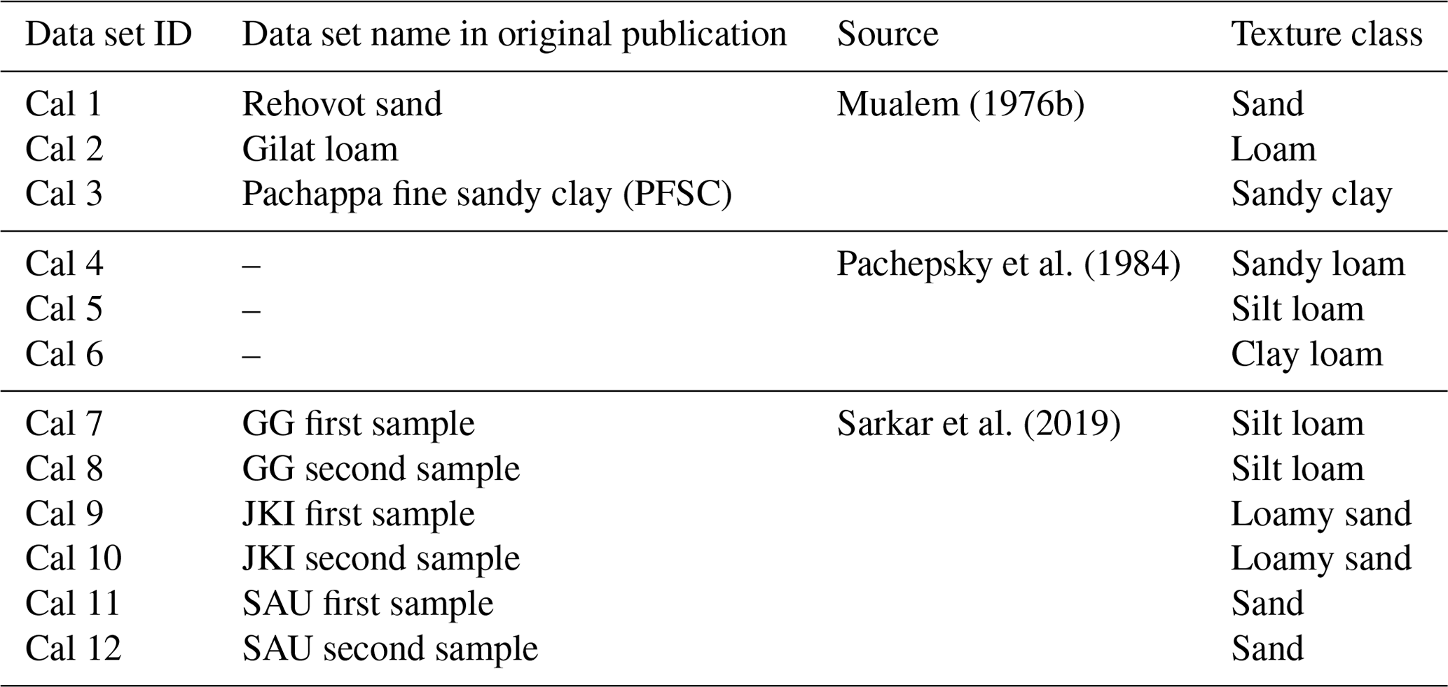
For each of the 16 model combinations, a model-specific τ_s was determined by fitting the WRC and HCC models to measured data. The adjustable parameters were all WRC parameters and τ_s. For the non-capillary conductivity, which becomes important in the medium to dry range, where film and corner flow is dominant, we used the prediction model of Peters et al. (2021). To obtain reliable estimates for τ_s, (i) data for the water retention function and (ii) hydraulic conductivity data in the wet range, but not at saturation, are required in high quality. We used the same 12 data sets that were already used by P23. The data encompass a wide variety of soil textures, from a pure sand to a clay loam. Details about the soils are given in the original literature and are summarized in Table 4.

Models were fitted to the data by nonlinear, weighted least-squares regression. The objective function was

$$\begin{array}{}\text{(18)}& \begin{array}{rl}& \mathit{\varphi }\left(\mathit{b}\right)=w_{\mathit{\theta }}\sum _{i=\mathrm{1}}^{n_{\mathit{\theta }}}{\left[{\mathit{\theta }}_i-{\stackrel{\mathrm{̃}}{\mathit{\theta }}}_i\left(\mathit{b}\right)\right]}^{\mathrm{2}}+\\ & w_{\mathrm{K}}\sum _{i=\mathrm{1}}^{n_K}{\left[{\log }_{\mathrm{10}}\left(K_i\right)-{\log }_{\mathrm{10}}\left({\stackrel{\mathrm{̃}}{K}}_i\left(\mathit{b}\right)\right)\right]}^{\mathrm{2}}.\end{array}\end{array}$$

Here, θ_i and ${\stackrel{\mathrm{̃}}{\mathit{\theta }}}_i$ are the measured and modeled water contents, K_i and ${\stackrel{\mathrm{̃}}{K}}_i$ are measured and modeled hydraulic conductivities, n_θ and n_K are the respective number of data points, w_θ=10 000 and w_K=16 are weights for the two data groups (Peters et al., 2011), and b is the vector of unknown model parameters. The SCE-UA algorithm (Duan et al., 1992) was applied to minimize the objective function. Details can be found in P23. Model performance was quantified by the root mean squared errors (RMSEs) of volumetric water content (WRC) and common log of K(h) (HCC).

Table 4 SHP data used for model fitting.

3.3 Testing the predictive performance of the models

The performance of the various HCC prediction schemes was tested by comparing purely predicted HCC functions with measured conductivity data. For this test, we used the same 23 validation data sets as P23. Details about the data are given in Table 5. The test data again comprise a broad range of different texture classes. The PDI retention model with the four basic saturation functions given in Table 3 was fitted to the water retention data, and the conductivity functions were predicted with the model-specific values of τ_s as determined through calibration.

Table 5 Data sets used to test the conductivity predictions.

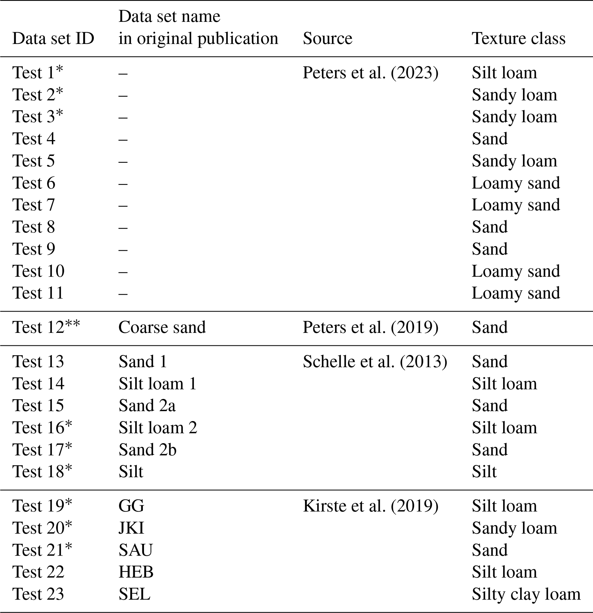
^∗ Samples taken at same sites but different years to some of the calibration data (Cal7 to Cal 12). ${}^{\ast \ast }$ Disturbed sample.

4 Results

4.1 Model-specific τ_s for the 16 model combinations

Figure 1 shows 4 out of the 12 calibration data sets and the corresponding fitted SHPs. We chose the FX-PDI model as the saturation function for illustration since P23 found that it performed best in describing the retention data. The fitted HCCs represent the four capillary bundle models tested. Overall, the differences between different WRC models and the associated conductivity curves are small (see Supplement). We limit Fig. 1 to four soils in order to keep the presentation concise; the corresponding graphs for all soils and all 16 model combinations are given in the Supplement.

The goodness of fit for the four models is quantified by the RMSE_θ and RMSE_logK (Fig. 2). The cut-and-random-rejoin models proposed by Mualem and CCG give rather small RMSEs for the retention as well as the conductivity curves, whereas the conceptually simpler models of Burdine and AS perform less well. Specifically, the AS model could often describe the conductivity data adequately, only at the expense of a poorer fit of the WRC data. Figure A1 shows the RMSE_θ and RMSE_logK box plots for all 16 model combinations, revealing that the specific findings for the FX basic function can be generalized.

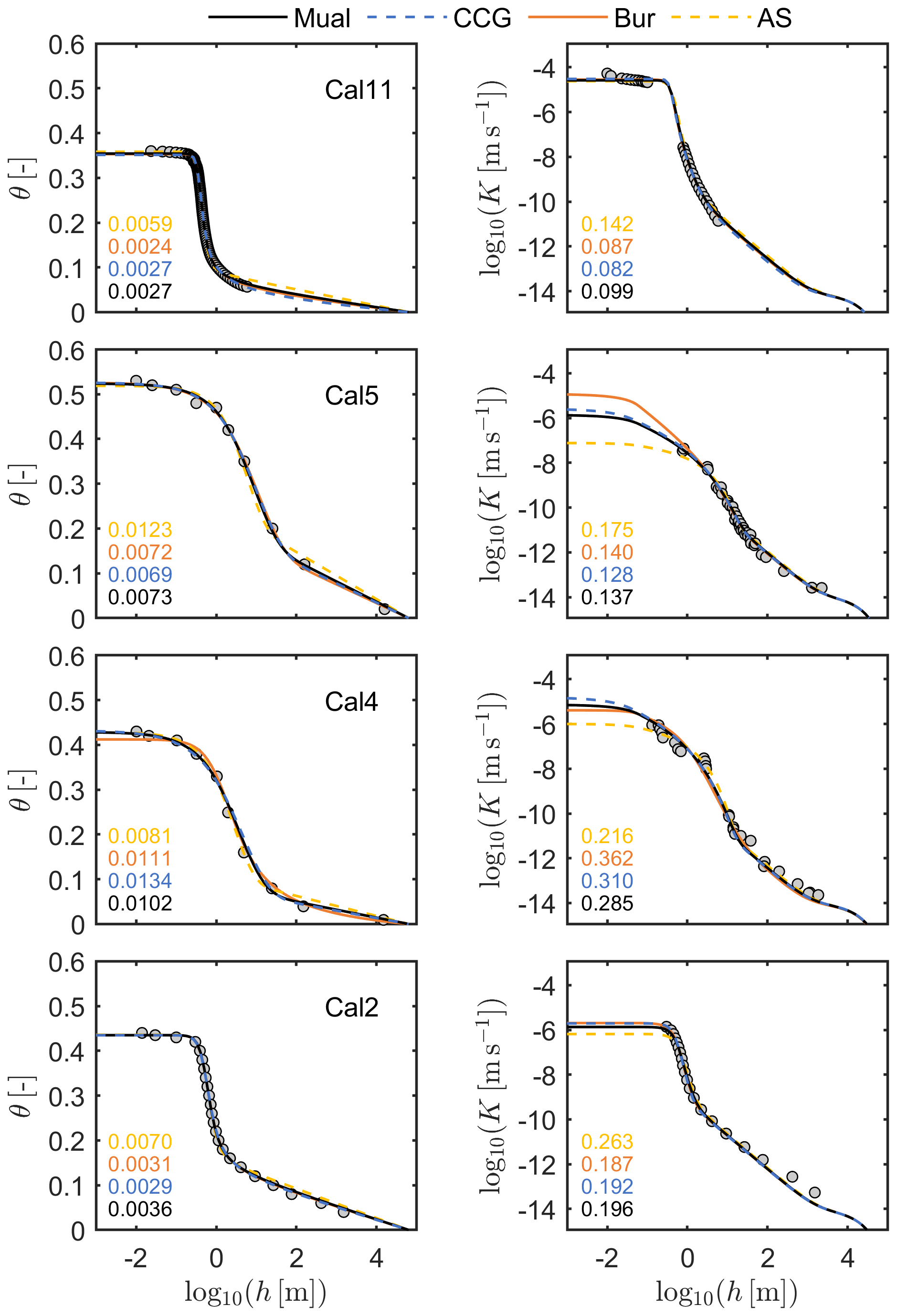
Figure 1 Plots of 4 of the 12 calibration data sets together with the fitted SHP functions. The FX-PDI model was used for WRC, and four capillary bundle models were used for the HCC. The estimated parameters were the five parameters of the FX-PDI and the saturated tortuosity coefficient τ_s. The numbers in the subplots indicate RMSE_θ and RMSE_logK values for the four models.

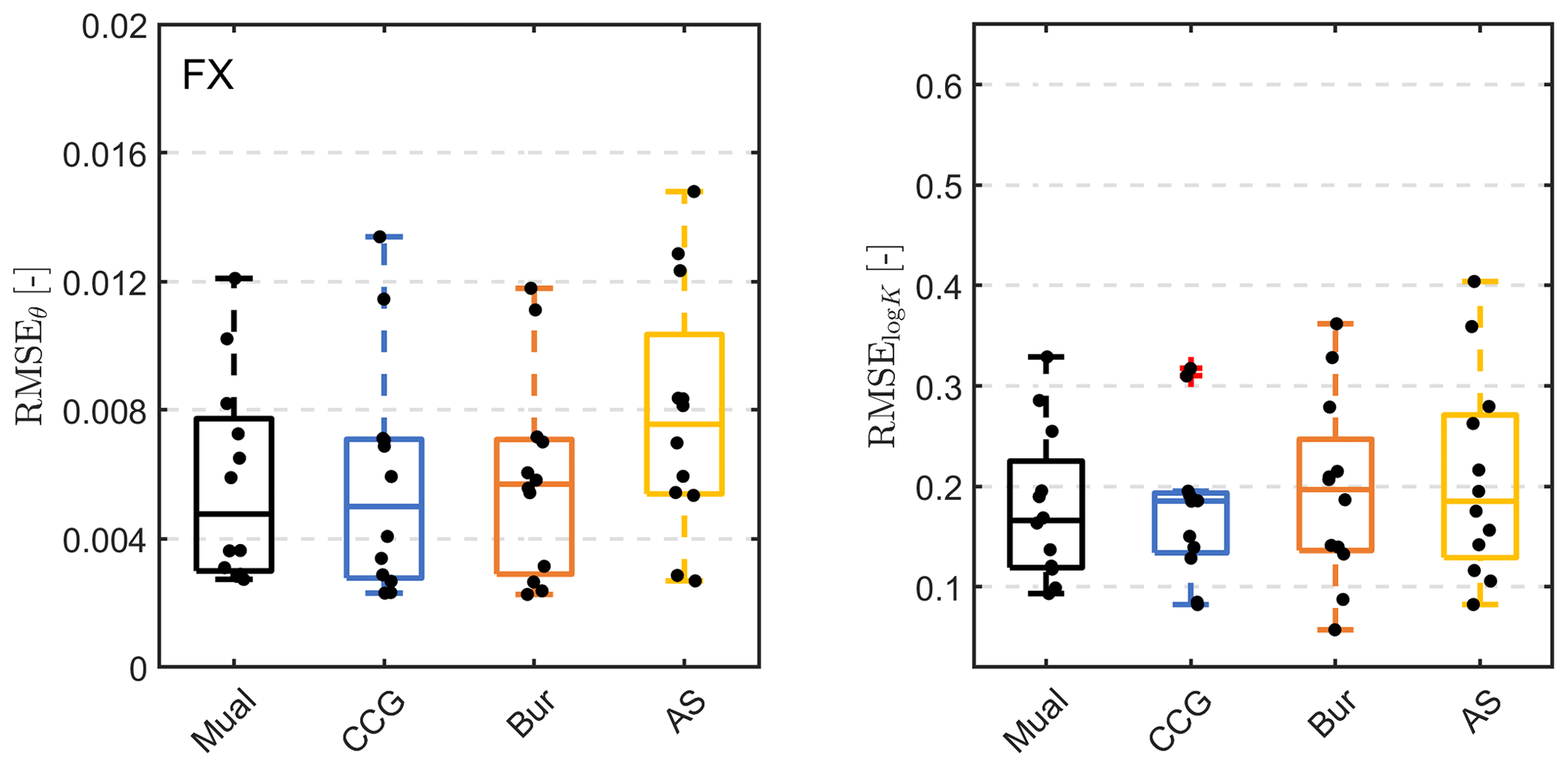
Figure 2 Distributions of RMSE_θ and RMSE_logK when fitting the FX-PDI retention model in combination with the four capillary conductivity functions listed in Table 2 to the 12 calibration data sets. Black dots indicate single realizations. The red cross indicates an outlier, defined by the MATLAB^® default settings as 1.5 times the interquartile range away from the top or bottom of the box (https://de.mathworks.com/help/matlab/ref/boxchart.html, last access: 15 December 2023).

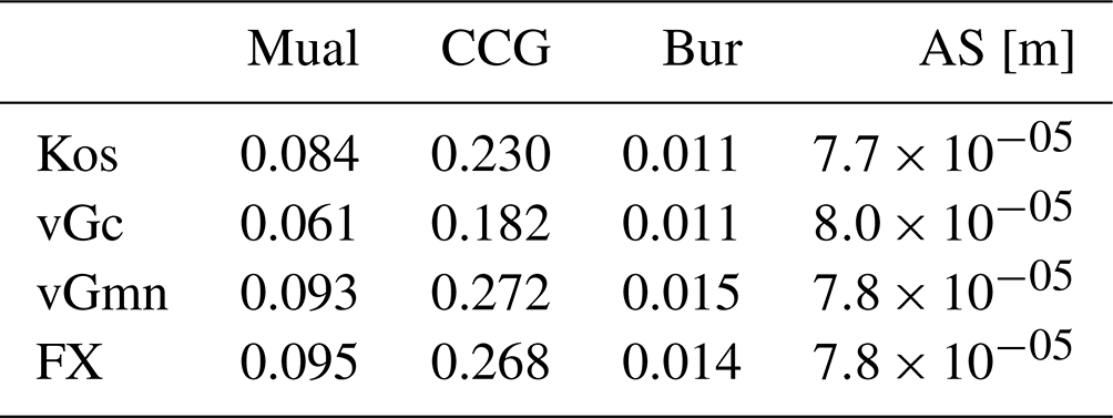
Figure 3 shows that the different conductivity prediction models give different optimal values for the saturated tortuosity coefficient, τ_s. This is in accordance with the discussion of the nature of τ_s in Peters et al. (2023), who acknowledge that the notion of a universally applicable saturated pore tortuosity is untenable. Rather, it must be seen as a general parameter in the context of the specific conceptualization of a capillary bundle model. The median values for τ_s are 0.095 for the Mualem model (as in P23), 0.27 for CCG, 0.014 for Burdine, and $\mathrm{7.8}\times {\mathrm{10}}^{-\mathrm{5}}$ for the AS model if the WRC is parameterized by the FX-PDI function. Note that τ_s has the unit [m] for the AS model, whereas it is dimensionless for the other models. Therefore, the absolute values of τ_s associated with the AS model cannot be directly compared numerically with the dimensionless coefficients of the other models; however, the spread on the log-scale is independent of the unit. The values of τ_s vary within a range of approximately 1.5 orders of magnitude for the Mual and CCG models, slightly less than 2 orders of magnitude for the Bur model, and more than 2 orders of magnitude for the AS model. The systematic differences of τ_s between the capillary bundle models can be attributed to the differing conceptual approaches implicit to these models, as the physical parameters of fluid properties are consistent, and the functional representation of the effective pore-size distribution was the same. We note that models based on Mual and CCG result in quite similar τ_s values, whereas those of the Bur model are a bit smaller. The AS model gives completely different values. Actually, the interpretation of τ_s in the AS model is difficult since part of the tortuosity is accounted for in the capillary model. Figure A2 shows the distributions of the τ_s values for all 16 model combinations. The medians of the estimated values for τ_s are summarized in Table 6.

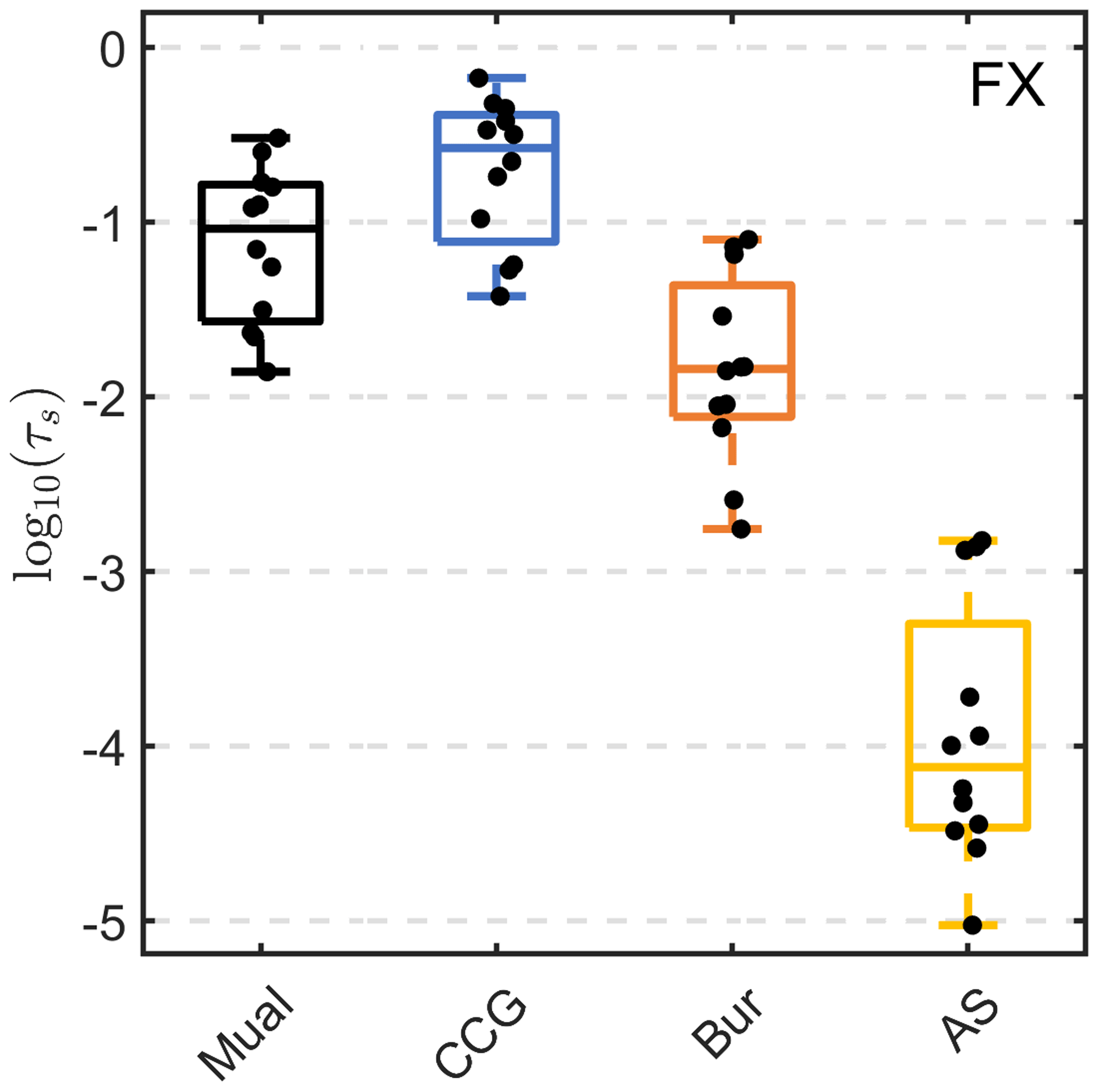
Figure 3 Distribution of optimal τ_s values obtained by fitting the four conductivity prediction models with the FX-PDI retention model to the 12 calibration data sets given in Table 4. Black dots indicate single realizations.

Table 6 Estimated values (median) of τ_s for all 16 model combinations.

4.2 Conductivity prediction accuracy by the different capillary bundle models

Fitting the retention models to the water retention data and using the values of τ_s obtained from the calibration (Table 6), we predicted the complete hydraulic conductivity functions for the 23 validation data sets and the 16 model combinations. Figure 4 shows the predicted functions and the data exemplarily for 6 out of the 23 data sets, again for the FX basic saturation model. With the exception of the AS model, the purely predicted conductivity curves agree remarkably well with the measured independent data. The curves for all data sets are given in the Supplement.

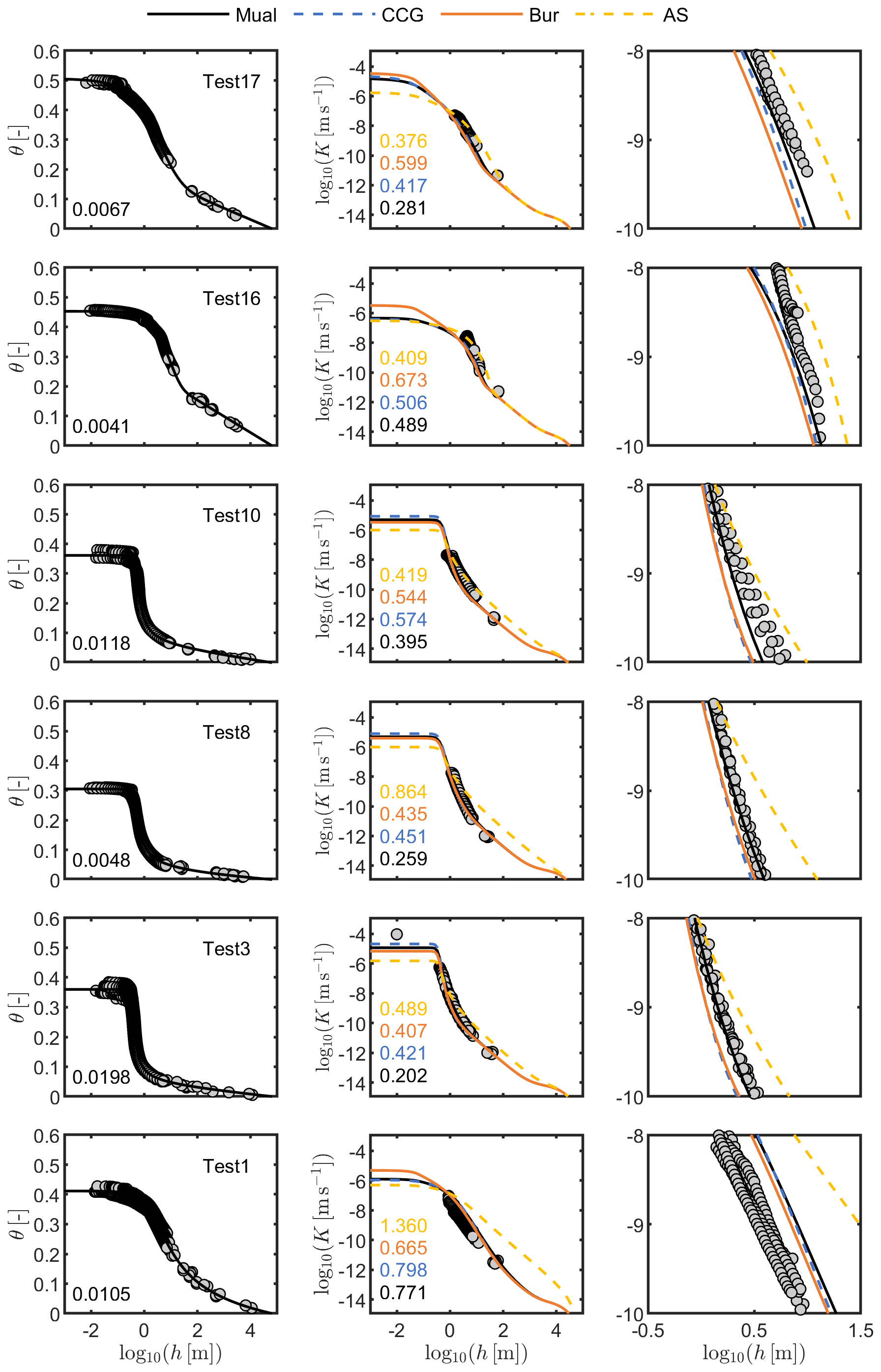
Figure 4 Measured data (dots), fitted retention functions (left) and predicted (not fitted) conductivity functions (center: complete curves; right: zoomed curves). Shown are six randomly selected soils out of 23 validation data sets. Numbers in the subplots indicate the RMSE_θ for the FX-PDI WRC model and the RMSE_logK values for the AS, Bur, CCG, and Mual conductivity models, from top to bottom.

Figure 5 shows the accuracy of the conductivity predictions again for the FX-PDI retention model, expressed by box plots of the RMSE_logK and the mean error (ME_logK). The distributions for all 16 model combinations are shown in Fig. A3. The median RMSE_logK in Fig. 5 is 0.40 for the Mual model, which yields the best prediction of all 16 model schemes. For the CCG model the median RMSE_logK is 0.42, and for the Bur model it is 0.44. For the AS model it is the worst, with a value of 0.66. Furthermore, the AS model leads to the largest variation in the prediction accuracy.

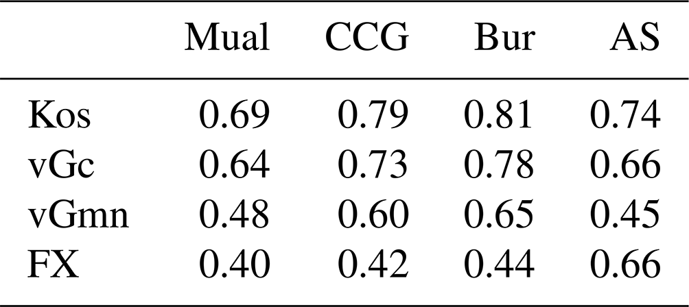
For all 16 model combinations (Fig. A3), the Mual model performed best for any of the investigated retention models. Table 7 lists the median RMSE_logK for all 16 model combinations. With the exception of the prediction that is based on the FX-PDI model, the median accuracy of the AS is as good or even better than the CCG and the Bur model. However, the AS prediction accuracy shows a large spread of RMSE_logK for any WRC model, with values up to 1.4 (Figs. 5, A3), which corresponds to a mismatch by a factor of 25 in the K values. Conversely, the Mual model performs not only well with respect to the median values but also yields the lowest spread for the RMSE_logK for any of the saturation functions; in other words it is the most robust. Figures 5 (right) and A3 indicate furthermore that only the combination of the FX capillary saturation function with the Mual capillary bundle model leads to unbiased results. Summarizing the above findings, the preferred model combination is the basic FX saturation model with Mualem's capillary conductivity model and τ_s=0.095. These results support the findings of van Genuchten and Nielsen (1985), Nimmo and Akstin (1988), and Kosugi (1999), who also found the Mualem model to perform best in their model comparisons.

The somewhat non-robust performance of the AS model, also found by Madi et al. (2018), can be explained by its assumption regarding tortuosity. We analyze this assumption in more detail in Appendix A4.

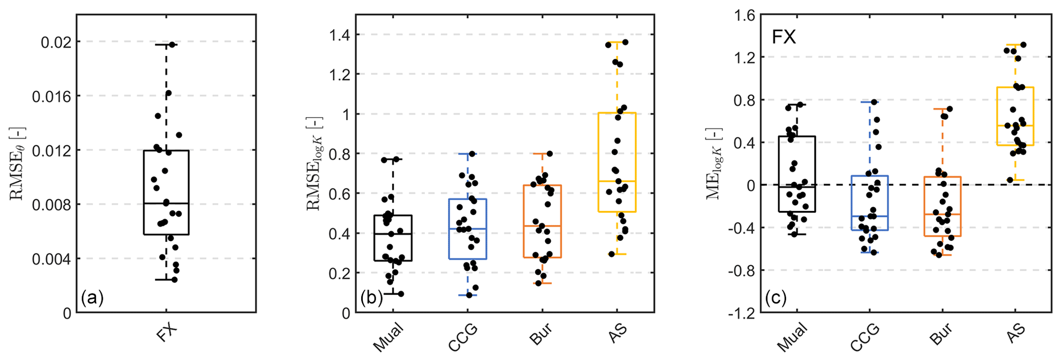
Figure 5 (a) RMSE_θ of the fitted PDI-FX retention model for the 23 test data sets. (b) and (c) RMSE_logK and mean errors of the predicted absolute conductivities by the four models listed in Table 2. Black dots indicate single realizations.

Table 7 Median of RMSE_logK for all model combinations.

4.3 Behavior of the capillary bundle models in the wet range

In the very wet moisture range, even tiny changes in the WRC can have a large impact on the HCC. Such small changes at arbitrary small suctions occur in common WRC parameterizations for soils with wide pore-size distributions or for bimodal soils. Durner (1994) concluded accordingly 3 decades ago that this makes a conductivity prediction based on statistical pore-bundle models in the range close to full saturation virtually impossible. In Fig. 6, we evaluate this effect for the four different conductivity prediction models. For illustration, we use the rather fine-textured silt loam (calibration data set 5, shown in Fig. 1, too) and show all model fits with and without consideration of a maximum pore size in the capillary bundle models (hclip, Iden et al., 2015), as described in Sect. 3.1.

In all cases, we fitted the retention model parameters and τ_s to the data. The fitted WRC (FX-PDI) values lie almost on top of each other (again with a slight difference for the AS model, as discussed in Sect. 4.3). The WRC fits differ slightly for the different model combinations, although we always used the same retention model because the retention parameters α, n, and m influence the shape of both hydraulic functions, which were simultaneously fitted by minimizing Eq. (2). The four conductivity models fit the given data similarly well but show a very different behavior in the wet moisture range, where no data are available. All models with the exception of the AS model show a strong increase of conductivity in the pressure range close to saturation in the unclipped version (dashed lines), from about h<0.01 m. This illustrates the artifact of using capillary bundle models without limiting the maximum pore size in the integrals used to calculate the conductivity function. In a classic approach where the relative conductivity function is predicted and matched to a measured or assumed value for K_s, the unsaturated conductivity curve would be underestimated markedly. The AS model appears to be least affected by this artifact.

However, even if the change of the HCC close to saturation caused by this artifact is removed by introducing a maximum pore size in the integrals (9) to (12), the four models differ markedly in their predicted shape in the moderately moist region (Fig. 6, “with clipping”; solid lines). The differences between the four models reach still almost 2 orders of magnitude, and they develop in a suction range where we are still far from unrealistically large pores sizes (recall that in the hclip curves, the maximum allowed pore diameter was 0.5 mm, corresponding to a suction of 0.06 m).

The reason for the varying behavior lies in the distinct pore-bundle models utilized. The Bur model, which assumes that the pore paths are parallel and tortuous, yields the greatest conductivity increase for large pores due to the Hagen–Poiseuille relationship with pore size. In contrast, the CCG and Mual models, which involve cutting and randomly rejoining most of the direct paths, mitigate this effect and exhibit comparable patterns. The AS model leads to the smallest change in hydraulic conductivity in the wet range.

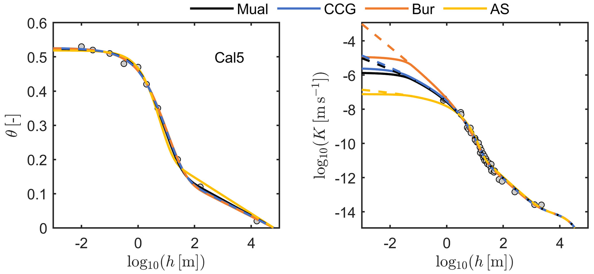
Figure 6 Fitted retention and conductivity functions with and without hclip to calibration set Cal 5. Solid lines: with clipping. Dashed lines: without clipping. Basic capillary saturation function is the FX model.

5 Summary and conclusion

In this study, we compared four different capillary bundle models in combination with four different unimodal capillary saturation models, leading to 16 model combinations, to predict the absolute hydraulic conductivity within the PDI model framework. For each of the 16 model combinations, we determined a model-specific value for the saturated tortuosity coefficient, τ_s, by fitting the models to a calibration data set. Using these general values of τ_s, we then predicted, for independent data sets, all three components of conductivity, namely isothermal vapor, non-capillary, and capillary liquid conductivity, from the WRC without any adjusted parameters, following Peters et al. (2021, 2023).

When predicting the HCC from the WRC, a good representation of the water retention function is essential; therefore, the best-performing model schemes were those that used the flexible three-parameter capillary saturation functions in the WRC model (i.e., the Fredlund and Xing, 1994, model and the unconstrained van Genuchten, 1980, model with independent parameters m and n).

Among the capillary bundle models, the cut-and-random-rejoin models introduced by Childs and Collis-George (1950) and Mualem (1976a) exhibited the best performance, with the Mualem model performing slightly superior. The Burdine (1953) model was less suited, while the model of Alexander and Skaggs (1986) performed the worst. The use of the AS model is, therefore, not recommended due to its unphysical representation of relative tortuosity. Since the model of Mualem (1976a) is mathematically simpler than the model of Childs and Collis-George (1950), we conclude that its establishment in soil hydrology is justified. The median RMSE_logK was 0.4 for the recommended FX-PDI-Mualem combination. In other words, the median relative error of the predicted K is about a factor of 2.6, which appears fair enough in the light of the expected measurement uncertainties.

It is interesting to note that even when fitted to the data, the various models exhibit distinct behavior near saturation during extrapolation. This can be attributed to differences in their model structures. Specifically, the Burdine model tends to overestimate the conductivity increase caused by the presence of even small amounts of water in large pores, as it directly applies the law of Hagen–Poiseuille to a specific pore diameter derived from the WRC. In contrast, the two cut-and-random-rejoin models result in a much smaller conductivity contribution from water stored in the largest pores due to the random combination of pores of different sizes. The AS model, on the other hand, appears to underestimate the conductivity increase in the wet range.

Our approach estimates the hydraulic conductivity of the soil matrix, excluding the influence of soil structure. It can be useful in situations without available conductivity data. When a measured value of saturated conductivity (K_s) is available, especially for topsoils where soil structure plays a significant role, combining our predicted hydraulic conductivity curve (HCC) with interpolation towards K_s can yield a well-defined conductivity function across the entire moisture range, as discussed in P23. This approach distinguishes between structural and textural effects, ensuring the consistent use of measured SHP information and allowing for the estimation of soil structure formation extent.

Appendix A

A1 The PDI model system

A1.1 PDI water retention function

The capillary saturation function S_c [-] and a non-capillary saturation function S_nc [-] may be superposed in the form (Peters, 2013; Iden and Durner, 2014)

$$\begin{array}{}\text{(A1)}& \mathit{\theta }\left(h\right)=({\mathit{\theta }}_{\mathrm{s}}-{\mathit{\theta }}_{\mathrm{r}})S_{\mathrm{c}}+{\mathit{\theta }}_{\mathrm{r}}{S}_{\mathrm{nc}},\end{array}$$

in which the first right term describes water stored in capillaries and the second term water stored in adsorbed water films and pore corners, θ [m³ m⁻³] is the total water content, h [m] is the suction head and θ_s [m³ m⁻³] and θ_r [m³ m⁻³] are the saturated and maximum adsorbed water contents, respectively. To meet the physical requirement that the capillary saturation function reaches zero at oven dryness, a basic saturation function Γ(h) is scaled by (Iden and Durner, 2014)

$$\begin{array}{}\text{(A2)}& S_{\mathrm{c}}\left(h\right)={\displaystyle \frac{\mathrm{\Gamma }\left(h\right)-\mathrm{\Gamma }\left(h_{\mathrm{0}}\right)}{\mathrm{1}-\mathrm{\Gamma }\left(h_{\mathrm{0}}\right)}},\end{array}$$

where h₀ [m] is the suction head at oven dryness, which can be set at 10^4.8 m following Schneider and Goss (2012). Γ(h) can be any uni- or multi-modal saturation function such as the unimodal functions of van Genuchten (1980) and Kosugi (1996) or their bimodal versions (Durner, 1994; Romano et al., 2011).

The saturation function for non-capillary water is given by a smoothed piecewise linear function (Iden and Durner, 2014), which is given here in the notation of Peters et al. (2021):

$$\begin{array}{}\text{(A3)}& S_{\mathrm{nc}}\left(h\right)={\displaystyle \frac{\ln \left(\frac{h_{\mathrm{0}}}{h}\right)-b\ln \left(\mathrm{1}+{\left[\frac{h_{\mathrm{a}}}{h}\right]}^{\mathrm{1}/b}\right)}{\ln \left(\frac{h_{\mathrm{0}}}{h_{\mathrm{a}}}\right)}}\end{array}$$

in which the parameter h_a [m] reflects the suction head where non-capillary water reaches its saturation (fixed in our study to the suction at which capillary saturation reaches 0.75). The derivation for h_a as a quantile of S_c is given in Peters et al. (2023), and the resulting mathematical expressions are listed below in Appendix A1.3. The parameter h₀ in Eq. (A3) is the suction head where the water content reaches zero, which reflects the suction at oven-dry conditions. S_nc(h) increases linearly from zero at oven dryness to its maximum value of 1.0 at h_a and then remains constant toward saturation. In order to ensure a continuously differentiable water capacity function, S_nc(h) must be smoothed around h_a, which is achieved by the smoothing parameter b [-] (Iden and Durner, 2014), given here by

$$\begin{array}{}\text{(A4)}& b=b_{\mathrm{o}}\left(\mathrm{1}+\mathrm{2}{\displaystyle \frac{\mathrm{1}-e^{-b_{\mathrm{1}}}}{n^{\mathrm{2}}}}\right),\end{array}$$

where b_o=0.1ln(10) and $b_{\mathrm{1}}={\left(\frac{{\mathit{\theta }}_{\mathrm{r}}}{{\mathit{\theta }}_{\mathrm{s}}-{\mathit{\theta }}_{\mathrm{r}}}\right)}^{\mathrm{2}}$.

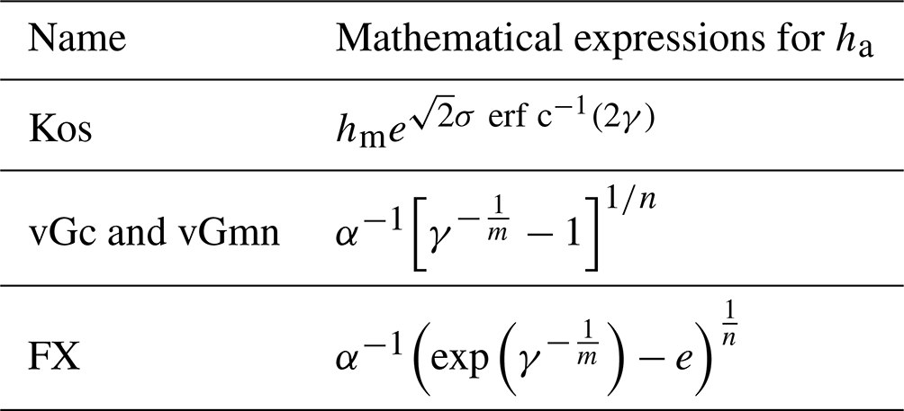
Table A1 Mathematical expressions for h_a for the capillary saturation functions used as derived by Peters et al. (2023). The parameter γ is given by $\mathit{\gamma }=\mathit{\xi }\left(\mathrm{1}-{\mathrm{\Gamma }}_{\mathrm{0}}\right)+{\mathrm{\Gamma }}_{\mathrm{0}}$, where ξ [-] is the chosen quantile of the capillary saturation for the derivation of h_a (in our case ξ is 0.75).

A1.2 PDI hydraulic conductivity

The PDI hydraulic conductivity model is expressed as (Peters et al., 2013)

$$\begin{array}{}\text{(A5)}& K\left(h\right)=K_{\mathrm{c}}+K_{\mathrm{nc}}+K_{\mathrm{v}},\end{array}$$

where K_c [-] [m s⁻¹], K_nc [m s⁻¹], and K_v [m s⁻¹] are the conductivities for the capillary, non-capillary, and isothermal vapor conductivities, respectively. K_nc is given by (Peters et al., 2021)

$$\begin{array}{}\text{(A6)}& K_{\mathrm{nc}}=c{\mathit{\theta }}_{\mathrm{m}}{h}_{\mathrm{a}}^{-\mathrm{1.5}}{\left({\displaystyle \frac{h_{\mathrm{0}}}{h_{\mathrm{a}}}}\right)}^{-\mathrm{1.5}(\mathrm{1}-S_{\mathrm{nc}})},\end{array}$$

in which c is used to account for several physical and geometrical constants and can be either a free fitting parameter to scale K_nc or $c=\mathrm{1.35}\times {\mathrm{10}}^{-\mathrm{8}}$ m${}^{\mathrm{5}/\mathrm{2}}$ s⁻¹. Parameter θ_m [-] is the water content at h=10³ m. We refer to Saito et al. (2006) or Peters (2013) for details regarding the formulation of K_v as a function of the invoked WRC. The conductivity for water flow in capillaries is described in this paper using the four pore bundle models summarized in Table 2.

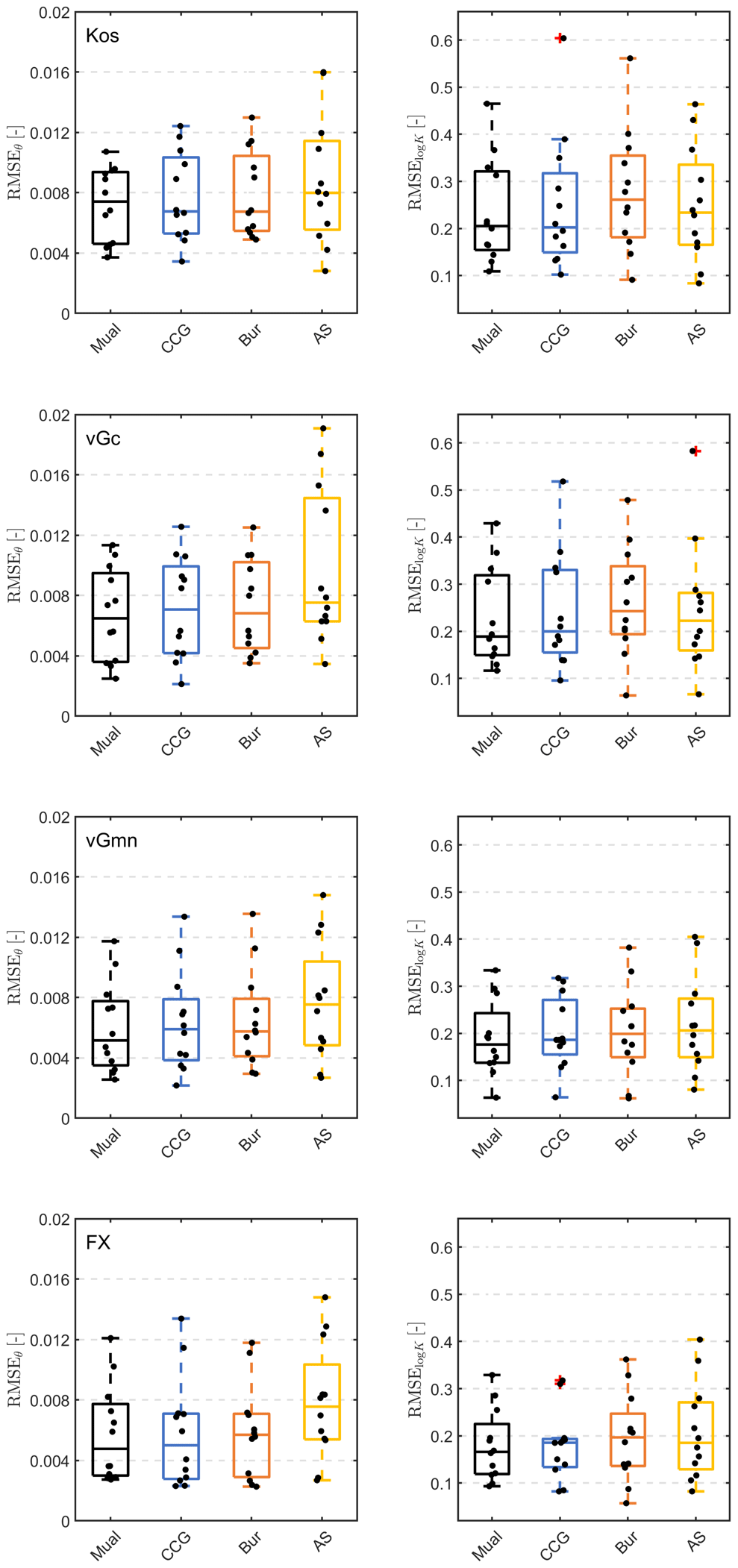
Figure A1 Distributions of RMSE_θ and RMSE_logK when fitting the four retention models in combination with the four capillary conductivity functions listed in Tables 2 and 3 to the 12 calibration data sets. First row: Kos as basic saturation function. Second row: vGc as basic saturation function. Third row: vGmn as basic saturation function. Fourth row: FX as basic saturation function. Black dots indicate single realizations. The red crosses indicate outliers, defined by the MATLAB^® default settings as 1.5 times the interquartile range away from the top or bottom of the box (https://de.mathworks.com/help/matlab/ref/boxchart.html, last access: 15 December 2023).

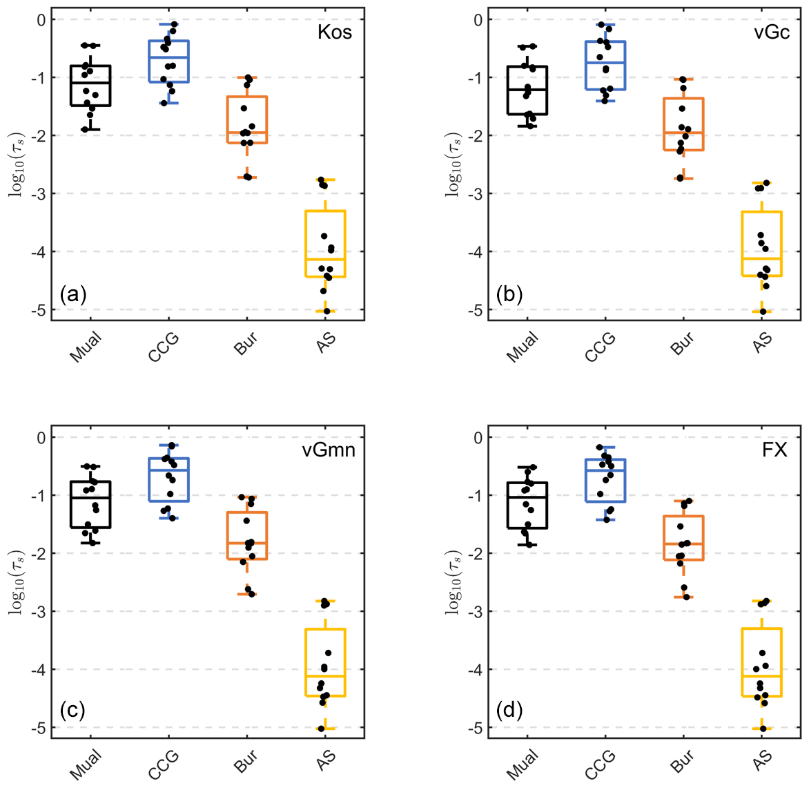
Figure A2 Distribution of fitted τ_s values for the four different capillary bundle models and the four basic capillary saturation functions fitted to the 12 data sets (see Fig. 6) given in Table 4. Black dots indicate single realizations. (a) Kos as basic saturation function, (b) vGc as basic saturation function, (c) vGmn as basic saturation function, and (d) FX as basic saturation function.

A1.3 Calculation of h_a

According to Peters et al. (2023), we set the air entry parameter for the non-capillary parts of the hydraulic functions, h_a, to the suction at which capillary saturation reaches 0.75. The expressions for the capillary saturation functions used are summarized in Table A1.

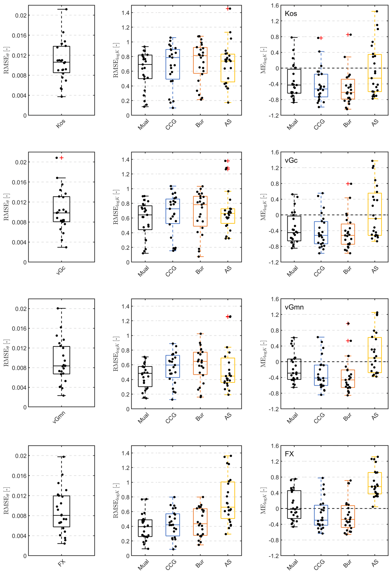
Figure A3 Left: RMSE_θ of the fitted PDI retention models for the 23 test data sets. Center and right: RMSE_logK and mean errors of the predicted absolute conductivities for all four different capillary bundle models and the four basic capillary saturation functions listed in Tables 2 and 3. Black dots indicate single realizations. First row: Kos as basic saturation function. Second row: vGc as basic saturation function. Third row: vGmn as basic saturation function. Fourth row: FX as basic saturation function. The red crosses indicate outliers, defined by the MATLAB^® default settings as 1.5 times the interquartile range away from the top or bottom of the box (https://de.mathworks.com/help/matlab/ref/boxchart.html, last access: 15 December 2023).

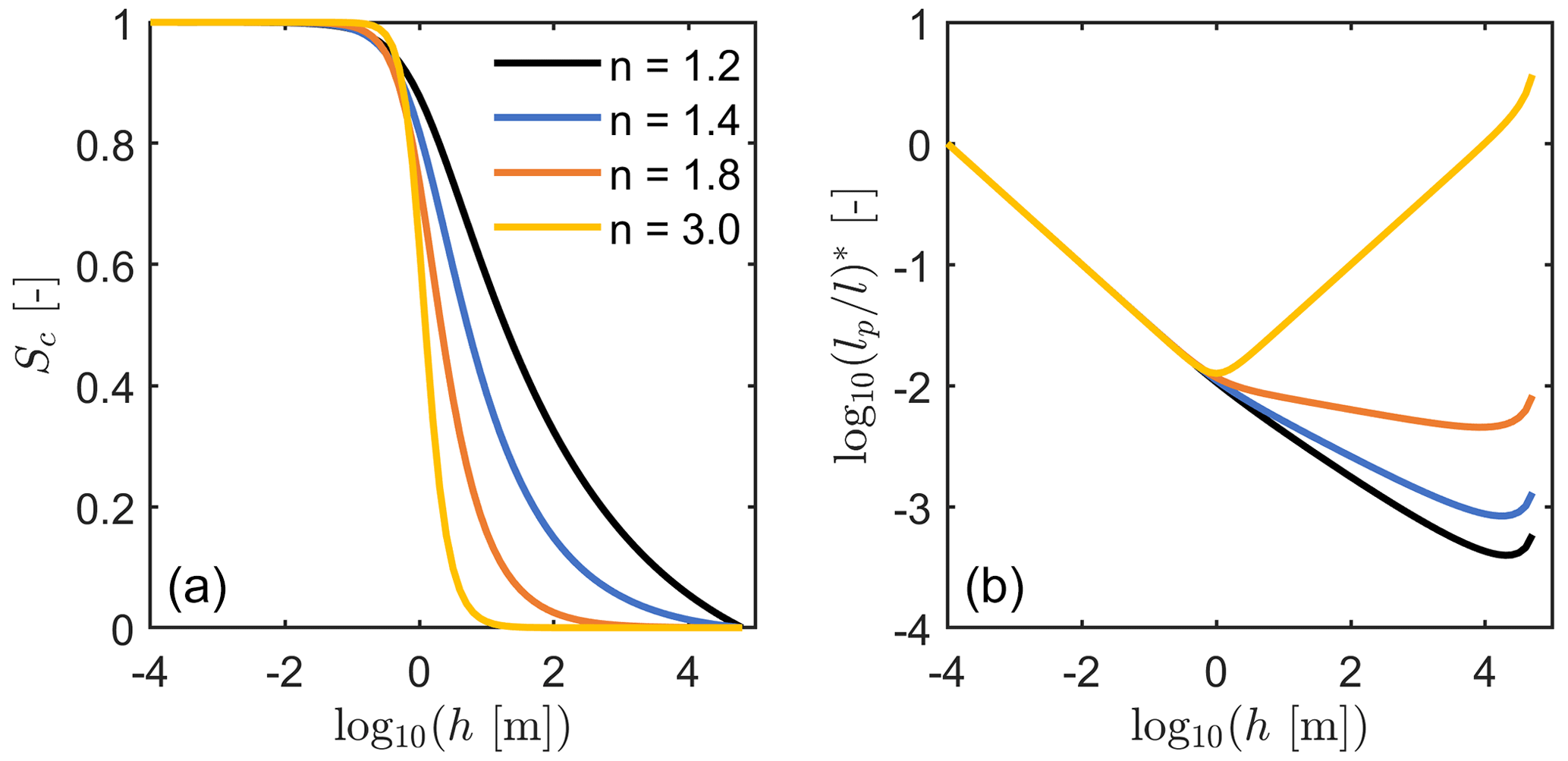
Figure A4 Scaled tortuosity correction used by AS conductivity prediction model for soils with different pore-size distributions. (a) Capillary saturation functions using the vGc saturation function with α=1.0 m⁻¹ and n varying from 1.2 to 3.0. (b) Associated scaled tortuosity correction $l_{\mathrm{p}}/l=C\sqrt{r/S_{\mathrm{c}}}$. Since we are only interested in the general shape of the function, we scaled $l_{\mathrm{p}}/l$ by assuming C=1 and dividing it by its value at $h={\mathrm{10}}^{-\mathrm{4}}$ m.

A2 Derivation of Alexander and Skaggs (1986) model

The capillary conductivity functions K_c(S_c) [L T⁻¹] given by a slightly modified version of Eq. (4) in Alexander and Skaggs (1986) are

$$\begin{array}{}\text{(A7)}& K_{\mathrm{c}}=\left({\mathit{\theta }}_{\mathrm{s}}-{\mathit{\theta }}_{\mathrm{r}}\right){\displaystyle \frac{\mathit{\rho }g}{\mathrm{8}\mathit{\eta }}}\underset{\mathrm{0}}{\overset{S_{\mathrm{c}}}{\int }}{r}^{\mathrm{2}}{\left({\displaystyle \frac{l}{l_{\mathrm{p}}}}\right)}^{\mathrm{2}}\mathrm{d}{\stackrel{\mathrm{̃}}{S}}_{\mathrm{c}},\end{array}$$

where θ_s [-] and θ_r [-] are the saturated and residual water contents; S_c [-] is the capillary saturation; ρ [kg m³] is the fluid density; g [m s²] is gravitational acceleration; η [N s m⁻²] is dynamic viscosity; r [m] is the radius of the capillary, which is assumed to have a circular cross-section; l [L] is the direct projection distance through the soil; l_p [m] is the path length for single water parcels; and ${\stackrel{\mathrm{̃}}{S}}_{\mathrm{c}}$ is the dummy variable of integration. The quotient $l_{\mathrm{p}}/l$ is the path elongation due to tortuosity. Note that for consistency, we use the maximum water-filled capillaries, θ_s−θ_r, instead of porosity, and the potential in the Hagen–Poiseuille law is given here in length units.

Applying the Young–Laplace relation, $r=\mathit{\kappa }/h$ with $\mathit{\kappa }=\mathrm{2}\mathit{\sigma }/\mathit{\rho }g$, where σ [N m⁻²] is the surface tension between the fluid and gas phases, and h [m] is the suction, leads to

$$\begin{array}{}\text{(A8)}& K_{\mathrm{c}}=\left({\mathit{\theta }}_{\mathrm{s}}-{\mathit{\theta }}_{\mathrm{r}}\right){\displaystyle \frac{\mathit{\rho }g}{\mathrm{8}\mathit{\eta }}}\underset{\mathrm{0}}{\overset{S_{\mathrm{c}}}{\int }}{\displaystyle \frac{{\mathit{\kappa }}^{\mathrm{2}}}{h^{\mathrm{2}}}}{\left({\displaystyle \frac{l}{l_{\mathrm{p}}}}\right)}^{\mathrm{2}}\mathrm{d}{\stackrel{\mathrm{̃}}{S}}_{\mathrm{c}}.\end{array}$$

Alexander and Skaggs (1986) assumed that the path elongation due to tortuosity, i.e., $l_{\mathrm{p}}/l$, depends on the saturation and the pore radius by

$$\begin{array}{}\text{(A9)}& l_{\mathrm{p}}/l=C\sqrt{r/S_{\mathrm{c}}},\end{array}$$

where C [m${}^{-\mathrm{1}/\mathrm{2}}$] is a constant, which is not further specified. Using the Young–Laplace relation leads to

$$\begin{array}{}\text{(A10)}& l_{\mathrm{p}}/l=C\sqrt{\mathit{\kappa }/\left(\mathrm{h}{S}_{\mathrm{c}}\right)}.\end{array}$$

Inserting Eq. (A10) into Eq. (A8) gives

$$\begin{array}{}\text{(A11)}& \begin{array}{rl}& K_{\mathrm{c}}=\left({\mathit{\theta }}_{\mathrm{s}}-{\mathit{\theta }}_{\mathrm{r}}\right){\displaystyle \frac{\mathit{\rho }g}{\mathrm{8}\mathit{\eta }}}\underset{\mathrm{0}}{\overset{S_{\mathrm{c}}}{\int }}{\displaystyle \frac{{\mathit{\kappa }}^{\mathrm{2}}}{h^{\mathrm{2}}}}{\displaystyle \frac{h{\stackrel{\mathrm{̃}}{S}}_{\mathrm{c}}}{C^{\mathrm{2}}\mathit{\kappa }}}\mathrm{d}{\stackrel{\mathrm{̃}}{S}}_{\mathrm{c}}\\ & =\left({\mathit{\theta }}_{\mathrm{s}}-{\mathit{\theta }}_{\mathrm{r}}\right){\displaystyle \frac{\mathit{\rho }g}{\mathrm{8}\mathit{\eta }}}\underset{\mathrm{0}}{\overset{S_{\mathrm{c}}}{\int }}{\displaystyle \frac{\mathit{\kappa }}{h}}{\displaystyle \frac{{\stackrel{\mathrm{̃}}{S}}_{\mathrm{c}}}{C^{\mathrm{2}}}}\mathrm{d}{\stackrel{\mathrm{̃}}{S}}_{\mathrm{c}}.\end{array}\end{array}$$

Substituting $\mathit{\kappa }=\mathrm{2}\mathit{\sigma }/\mathit{\rho }g$ yields

$$\begin{array}{}\text{(A12)}& K_{\mathrm{c}}=\left({\mathit{\theta }}_{\mathrm{s}}-{\mathit{\theta }}_{\mathrm{r}}\right){\displaystyle \frac{\mathit{\sigma }}{\mathrm{4}\mathit{\eta }}}{\displaystyle \frac{\mathrm{1}}{C^{\mathrm{2}}}}\underset{\mathrm{0}}{\overset{S_{\mathrm{c}}}{\int }}{\displaystyle \frac{S_{\mathrm{c}}}{h}}\mathrm{d}{\stackrel{\mathrm{̃}}{S}}_{\mathrm{c}}.\end{array}$$

Since h is a function of S_c, Eq. (A12) can be solved using partial integration, which leads to

$$\begin{array}{}\text{(A13)}& K_{\mathrm{c}}=\left({\mathit{\theta }}_{\mathrm{s}}-{\mathit{\theta }}_{\mathrm{r}}\right){\displaystyle \frac{\mathit{\sigma }}{\mathrm{4}\mathit{\eta }}}{\displaystyle \frac{\mathrm{1}}{C^{\mathrm{2}}}}\left\{S_{\mathrm{c}}\underset{\mathrm{0}}{\overset{S_{\mathrm{c}}}{\int }}{\displaystyle \frac{\mathrm{1}}{h}}\mathrm{d}{\stackrel{\mathrm{̃}}{S}}_{\mathrm{c}}-\underset{\mathrm{0}}{\overset{S_{\mathrm{c}}}{\int }}\underset{\mathrm{0}}{\overset{S_{\mathrm{c}}}{\int }}{\displaystyle \frac{\mathrm{1}}{h}}\mathrm{d}{\stackrel{\mathrm{̃}}{S}}_{\mathrm{c}}\mathrm{d}{\stackrel{\mathrm{̃}}{S}}_{\mathrm{c}}\right\}.\end{array}$$

Alexander and Skaggs neglected the last term in the curly brackets, which leads to

$$\begin{array}{}\text{(A14)}& K_{\mathrm{c}}=\left({\mathit{\theta }}_{\mathrm{s}}-{\mathit{\theta }}_{\mathrm{r}}\right){\displaystyle \frac{\mathit{\sigma }}{\mathrm{4}\mathit{\eta }}}{\displaystyle \frac{\mathrm{1}}{C^{\mathrm{2}}}}{S}_{\mathrm{c}}\underset{\mathrm{0}}{\overset{S_{\mathrm{c}}}{\int }}{\displaystyle \frac{\mathrm{1}}{h}}\mathrm{d}{\stackrel{\mathrm{̃}}{S}}_{\mathrm{c}}.\end{array}$$

In our notation, τ_s is given by $\mathrm{1}/C^{\mathrm{2}}$ and has the unit [m], and the parameter β is replaced by ${\mathit{\beta }}^{\prime }=\mathit{\sigma }/\mathrm{4}\mathit{\eta }$, which finally leads to

$$\begin{array}{}\text{(A15)}& K_{\mathrm{c}}={\mathit{\beta }}^{\prime }{\mathit{\tau }}_{\mathrm{s}}{S}_{\mathrm{c}}\left({\mathit{\theta }}_{\mathrm{s}}-{\mathit{\theta }}_{\mathrm{r}}\right)\underset{\mathrm{0}}{\overset{S_{\mathrm{c}}}{\int }}{\displaystyle \frac{\mathrm{1}}{h}}\mathrm{d}{\stackrel{\mathrm{̃}}{S}}_{\mathrm{c}}.\end{array}$$

A3 Results for all model combinations

A4 Analyzing the tortuosity assumption of Alexander and Skaggs (1986)

Physically, the path elongation due to tortuosity $l_{\mathrm{p}}/l$ should strictly increase with decreasing saturation. In the AS model it is assumed to follow $l_{\mathrm{p}}/l=C\sqrt{r/S_{\mathrm{c}}}$. Figure A4 visualizes the relationship between tortuosity and pressure head for four different capillary saturation functions, which reflect differently wide pore-size distributions. The path elongation, $l_{\mathrm{p}}/l$, plotted as relative function ${\left(l_{\mathrm{p}}/l\right)}^{\ast }$, decreases with increasing h (decreasing saturation), which is unphysical. The only exception is found for the very narrow pore-size distribution in the range beyond the air-entry point. When fitting the WRC and HCC simultaneously, this behavior of the AS conceptual model is counteracted by a worse fit of the retention data (see Figs. 1 and 2). In a pure prediction, where only the retention model is fitted, this can lead to a bad performance of the conductivity prediction. Similar to our results, Madi et al. (2018), who used the measured saturated conductivity for scaling, found that the AS model severely overestimates the unsaturated conductivity for most soils.