Investigating sources of variability in closing the terrestrial water balance with remote sensing

Remote sensing (RS) data are becoming an increasingly important source of information for water resource management as they provide spatially distributed data on water availability and use. However, in order to guide appropriate use of the data, it is important to understand the impact of the uncertainties of RS data on water resource studies. Previous studies have shown that the degree of closure of the water balance from remote sensing data is highly variable across basins and that different RS products vary in their levels of accuracy depending on climatological and geographical conditions.

In this paper, we analyzed the water-balance-derived runoff from global RS products for 931 catchments across the globe. We compared time series of runoff estimated through a simplified water balance equation using three precipitation (CHIRPS, GPM, and TRMM), five evapotranspiration (MODIS, SSEBop, GLEAM, CMRSET, and SEBS), and three water storage change (GRACE-CSR, GRACE-JPL, and GRACE-GFZ) RS datasets with monthly in situ discharge data for the period 2003–2016. Results were analyzed through the lens of 10 quantifiable catchment characteristics in order to investigate correlations between catchment characteristics and the quality of RS-based water balance estimates of runoff and whether specific products performed better than others under certain conditions.

The median Nash–Sutcliffe efficiency (NSE) for all gauges and all product combinations was −0.02, and only 44.9 % of the time series reached a positive NSE. A positive NSE could be obtained for 73.7 % of stations with at least one product combination, while the overall best-performing product combination was positive for 58.4 % of stations. This confirms previous findings that the best-performing products cannot be globally established. When investigating the results by catchment characteristic, all combinations tended to show similar correlations between catchment characteristics and the quality of estimated runoff, with the exception of combinations using MODIS evapotranspiration, for which the correlation was frequently reversed. The combinations with the GPM precipitation product generally performed worse than the CHIRPS and TRMM data. However, this can be attributed to the fact that the GPM data are available at higher latitudes compared to the other products, where performance is generally poorer. When removing high-latitude stations, this difference was eliminated, and GPM and TRMM showed similar performance.

The results show the highest positive correlation between highly seasonal rainfall and runoff NSE. On the other hand, increasing snow cover, altitude, and latitude decreased the ability of the RS products to close the water balance. The catchment's dominant climate zone was also found to be correlated with time series performance, with the tropical areas providing the highest (median NSE = 0.11) and arid areas the lowest (median NSE = −0.09) NSE values. No correlation was found between catchment area and runoff NSE. The results highlight the importance of further studies on the uncertainties of the different data products and how these interact when combining them, as well as of new approaches to using the data rather than simple water-balance-type approaches. Efforts to improve specific satellite products can also be better targeted using the results of this study.

1 Introduction

With an increasing global population and pressure on the available water resources, it is increasingly important to understand the spatial and temporal distribution of water resource availability and use. Quantifying the components of the water balance is a necessary first step in sustainably managing resources in a river basin or catchment. However, the data available in many river basins are insufficient to make informed water management decisions. Global monitoring of discharge, which is one of the key variables of interest to water managers, has been in decline since the 1980s (Vorosmarty et al., 2001). In addition, even where in situ data exist, the accessibility of the data can be problematic.

This data gap is increasingly being filled by remote sensing products, which provide many advantages (see, e.g., Sheffield et al., 2018 for a full review). For instance, remote sensing data can give valuable insights into the spatial variability of water availability and consumption, which can be difficult or impossible to obtain through in situ data collection. Utilizing the hydrological variables currently derived from remote sensing, it is now theoretically possible to close the water balance and to estimate runoff at the regional to global scale. However, due to uncertainties and errors in remote sensing data, this cannot currently be achieved at the scales and precision necessary for decision making (Sheffield et al., 2018).

Runoff estimation using remote sensing is typically done using some form of the following water balance equation (Eq. 1) (see, e.g., Syed et al., 2005):

$$\begin{array}{}\text{(1)}& \mathrm{Ro}=P-{\mathrm{ET}}_{\mathrm{a}}-{\displaystyle \frac{\mathrm{d}S}{\mathrm{d}t}},\end{array}$$

where Ro is total runoff, P is the precipitation, ET_a is the actual evapotranspiration, and $\mathrm{d}S/\mathrm{d}t$ is the total water storage change. Of the quantities in Eq. (1), all but the total runoff, which includes surface and subsurface components, can be derived from remote sensing at the global scale: remote sensing precipitation has been available for many years and is routinely used as input to hydrological models (see, e.g., Stisen and Sandholt, 2010); ET_a is not a direct RS (remote sensing) measurement, but many different algorithms have been developed to produce global scale ET_a from RS data (Zhang et al., 2016), and total water storage change can be monitored using measurements of the variation of the Earth's gravitational field by the Gravity Recovery and Climate Experiment (GRACE, Wahr et al., 2004). We note that, given adequate auxiliary information (such as, for example, bathymetry or rating curves), discharge can be monitored using radar altimetry (see, e.g., Kouraev et al., 2004; Michailovsky et al., 2012). However, currently (2023), neither the radar altimetry nor the auxiliary information is available consistently at the global scale, and in situ or modeled data are therefore necessary in order to assess the closure of the water balance using Eq. (1).

A common approximation made when analyzing the terrestrial water budget using remote sensing over a hydrological basin or sub-catchment is to equate the total runoff with the discharge leaving the area of study. This is equivalent to the assumption that subsurface fluxes in and out of the basin are negligible. While this assumption is likely to have an impact, particularly for studies at small spatial scales (see, e.g., Bouaziz et al., 2018; Fan and Schaller, 2009), it allows for the use of in situ discharge data to evaluate the reliability of the remote sensing inputs to Eq. (1), which is then rewritten as Eq. (2):

$$\begin{array}{}\text{(2)}& Q=P-{\mathrm{ET}}_{\mathrm{a}}-{\displaystyle \frac{\mathrm{d}S}{\mathrm{d}t}}.\end{array}$$

For the components of the water cycle which are available through RS, various datasets are available, and each product is subject to uncertainties and errors. These include the fact that most remote sensing measurements are indirect, therefore requiring interpretation and calibration; subject to interference (e.g., by cloud cover and topography); and limited in their spatial and temporal resolution relative to the phenomena measured. Each product uses its own algorithms, gap-filling procedure, parameterization, and validation methods to produce the variable of interest. Studies have shown that there is large variability between the different products for a single variable (e.g., Sahoo et al., 2011).

Previous studies have analyzed the closure of the water balance with remote sensing and other global datasets from the regional to global scale. The first of such studies was performed by Syed et al. (2005), who used the land–atmosphere water balance to estimate discharge over the Amazon and Mississippi River basins using data from the European Centre for Medium-Range Weather Forecasts (ECMWF) and from GRACE to measure water storage change. They found that the total basin outflow was well correlated with observed streamflow in spite of phase (in the Amazon) and amplitude (in the Mississippi) discrepancies. Sheffield et al. (2009) also analyzed the water budget closure for the Mississippi and found that the RS-estimated discharge was greatly overestimated. Sahoo et al. (2011) estimated the water budget from remote sensing and in situ discharge gauges over 10 global river basins and found errors in the runoff estimates of the order of 5 % to 25 % of the mean annual precipitation values. Both Sheffield et al. (2009) and Sahoo et al. (2011) concluded that the largest contributors to the lack of closure of the water balance were errors and biases in the precipitation products used.

At the global scale, one of the most comprehensive studies of the closure of the water balance from global products (including remote sensing products and products derived from gauges and models) was carried out by Lorenz et al. (2014). They compared the ability of combinations of five precipitation products (four derived from gauges and one including RS and gauge measurements), six evapotranspiration (ET) products (including MOD16 and GLEAM from RS), and two storage change solutions from GRACE (GFZ and CSR) over 96 catchments spread around the world. No single product combination was found to consistently outperform the others across catchments, but catchments with high seasonality tended to show better results.

More recently, Lehmann et al. (2022) performed a similar analysis on 189 river basins covering 90 % of the global land surface and analyzed combinations of 11 precipitation and 14 ET datasets and 11 runoff datasets (including data from land surface models, gauge products, and reanalysis datasets) and compared the computed storage change to GRACE data. They found that 95 % of basins had a positive Nash–Sutcliffe efficiency (NSE) for at least one product combination. They considered two catchment characteristics in analyzing their results and found that, while no correlation between catchment area and closure of the water balance could be found, there was a correlation between climatic zone and performance for some of the datasets considered.

Other studies compared runoff computations obtained from different remote sensing input datasets to assess the best product combinations in specific regions. For example, Moreira et al. (2019) computed runoff using Eq. (2) over South America using two precipitation products (TRMM and MSWEP), two ET products (MOD16 and GLEAM), and three storage change solutions from GRACE (CSR, JPL, and GFZ) and found that using GLEAM for ET estimation and MSWEP for precipitation produced the best results. They also reported that greater biases were found in semi-arid basins with low runoff coefficients.

Following the findings from previous studies that different catchment characteristics (e.g., climate and seasonality) and different product combinations produced different results, this study aims to investigate both the ability of different combinations of RS products to reproduce in situ measurements of discharge and to identify catchment characteristics that affect how well the closure of the water balance can be achieved among a wider range of catchment characteristics than those considered in previous studies. This is necessary in order to help water practitioners choose between different remote sensing datasets as the use of RS becomes more widespread in water balance assessments, as well as to better understand the sources of uncertainties present in the different products and to identify areas of improvement. In order to do this, 45 combinations of RS products (three precipitation products, five ET products, and three water storage change products) were used as input to the water balance equation (Eq. 2), and the discharge values computed were compared to discharge data collected from the Global Runoff Data Center (GRDC, 2019) over between 595 and 931 catchments (the number of catchments analyzed for each product combination varied due to coverage extent differences between products). The results were then analyzed using 10 quantifiable catchment characteristics to identify potential drivers of the goodness of fit between computed and in situ values.

2 Methodology

The ability of different remote sensing product combinations to correctly close the water balance was assessed by deriving runoff time series for each combination of products using the water balance equation of a river basin (see Eq. 2) and comparing these RS-derived runoff values with monthly time step discharge measurements obtained from the Global Runoff Data Centre (GRDC) for a period of 14 years, for which the RS products are consistently available.

The main drivers for the goodness of fit between calculated and observed runoff were investigated by evaluating 10 quantifiable basin characteristics.

2.1 Remote sensing data

The data needed to solve the water balance for runoff are total water storage change, precipitation, and actual evapotranspiration (see Eq. 2) over the study period. These time series were acquired from a variety of global remote sensing products: three different precipitation products, five actual evapotranspiration products, and three total water storage change products. An overview of these products is shown in Table 1, and details of the products are provided in the following sections.

Table 1 Overview of the different remote sensing products acquired.

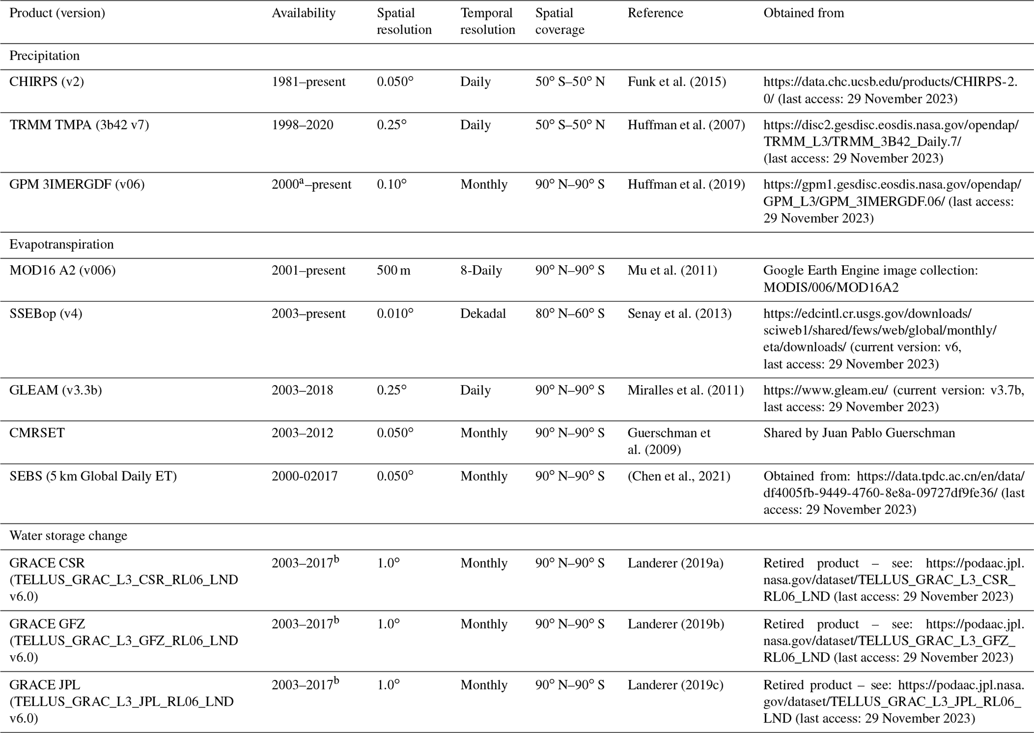
^a The TRMM mission ended in 2015, but the TMPA product continued to be produced using data from GPM; the GPM satellite was launched in 2015, but the IMERG product
started in 2000 using TRMM data. ^b The GRACE mission produced data until July 2017, and the GRACE-FO satellite started producing data from June 2018.

Data were collected for a period of 14 years between 2003 and 2016, which are the full years for which the storage change from the Gravity Recovery and Climate Experiment (GRACE) data is available. All the products used are available within this time frame, except for CMRSET, which was discontinued at the end of 2012.

The products cover most of the globe (see spatial coverage in Table 1). CHIRPS and TRMM do not cover areas north of 50^∘ N and south of 50^∘ S, meaning that Antarctica and the northern parts of Canada and Russia are excluded. The spatial extent of SSEBop is also limited to areas between 80^∘ N and 60^∘ S. Furthermore, it is important to note that SEBS has many missing pixels, mainly over the larger deserts, such as the Sahara and the Arabian Desert, as well as the Taiga in Canada and Russia.

All the products were re-sampled to a monthly timescale and to a spatial resolution of 0.05^∘ (specific methods are detailed in the following sections), and pixel values were weighted by area before computing the time series to account for the changing pixel areas at different distances from the Equator. The analysis focused on spatial aggregates of runoff for catchments larger than 10 000 km², and the spatial resampling was therefore not expected to have a large impact on the results. For studies which focus on smaller scales or the pixel level, the impact of spatial resampling would need to be carefully considered. The choice of a monthly timescale was motivated by the timescales of the available remote sensing, particularly the GRACE dataset.

2.1.1 Precipitation

Different sensors and algorithms are used to estimate global precipitation from remote sensing. Many of the available precipitation products combine measurements from sensors aboard multiple satellites in order to be able to achieve higher temporal resolutions, and some products are merged with in situ gauge data to improve accuracy (Sheffield et al., 2018). In this study, the following three products were used:

• the Tropical Rainfall Measuring Mission (TRMM) Multi-satellite Precipitation Analysis (TMPA) 3B42 product (Huffman et al., 2007)

• the Climate Hazards group Infrared Precipitation with Stations (CHIRPS) version 2 product (Funk et al., 2015)

• the Global Precipitation Measurement (GPM) mission Integrated Multi-satellitE Retrievals for GPM (IMERG) final run (Huffman et al., 2019).

The datasets had to be resampled from their native resolutions (see Table 1) to obtain monthly data at 0.05^∘ spatial resolution:

• The TRMM TMPA and GPM IMERG products were resampled to 0.05^∘ using the nearest-neighbor method.

• The daily TRMM and CHIRPS daily data products were summed to obtain monthly values.

It should be noted that the products used are in large part computed from the same source satellite measurements. In particular, while the core GPM satellite was launched in February 2014, the IMERG algorithm was used to extend the time series back to June 2000 using data from the TRMM era to produce a continuous long-term dataset.

2.1.2 Evapotranspiration

Evapotranspiration (ET) obtained from RS data is not a direct measurement, and many different inputs are required for models to be able to represent the biophysical and environmental controls on ET (see, e.g., Zhang et al., 2016). Five different evapotranspiration products have been used to solve the water balance for runoff in this study¹:

• the Operational Simplified Surface Energy Balance (SSEBop, Senay et al. 2013)

• CSIRO MODIS Reflectance-based Evapotranspiration (CMRSET, Guerschman et al., 2009)

• the Global Land Evaporation Amsterdam Model (GLEAM, Miralles et al., 2011).

• Surface Energy Balance System (SEBS, Chen et al., 2021)

• MODIS Global Terrestrial Evapotranspiration Algorithm (MOD16, Mu et al., 2011).

These products use different methods and data sources for estimating evapotranspiration rates. For example, the MOD16 algorithm is based on the Penman–Monteith equation, CMRSET and GLEAM use modified versions of the Priestly–Taylor equation, while SSEBop and SEBS use surface energy balance approaches. More details can be found in the publications listed for each product.

In order to obtain monthly data at 0.05^∘ spatial resolution from the resolutions listed in Table 1, the following was done:

• The daily and dekadal (10 d) fluxes from SSEBop and GLEAM were summed to obtain monthly values.

• The 8-daily data from MOD16 were summed to monthly values (with reduced weights for images partially within a specific month). Missing data within a month were filled by setting the missing data to the monthly average of the available 8-day evapotranspiration in that month.

• MOD16, SSEBop, and GLEAM were resampled to 0.05^∘ using the nearest-neighbor method.

2.1.3 Storage change

Total water storage (the sum of surface and subsurface water storage) cannot be directly measured from remote sensing. However, total water storage anomalies (TWSAs), i.e., the deviation in total water storage relative to the long-term mean, can be obtained from the Gravity Recovery And Climate Experiment (GRACE) satellites, which map the Earth's gravity field approximately every 30 d (Biancamaria et al., 2019).

Table 2 Catchment characteristics considered in this study.

The TELLUS GRACE Level-3 Monthly Land Water-Equivalent-Thickness Surface Mass Anomaly release 6.0 products from three processing centers were used in this study (Landerer and Swenson, 2012):

• the University of Texas – Center for Space Research (CSR, Landerer, 2019a)

• GeoForschungsZentrum (GFZ, Landerer, 2019b)

• Jet Propulsion Laboratory (JPL, Landerer, 2019c).

GRACE data are available between January 2003 and July 2017. The data are available in quasi-monthly time steps with variable windows of observation. However, most of the data are centered on the 16th of each month. The data were interpolated to the 16th day of every month, and the central-difference method was used to calculate the change in storage (see, e.g., Biancamaria et al., 2019). Finally, the data were resampled to 0.05^∘ using the nearest-neighbor method.

2.2 In situ data: Global Runoff Data Centre

The RS-derived runoff was validated using observed runoff from the Global Runoff Data Centre (GRDC), whose dataset comprises more than 9900 gauging stations all over the world. By filtering to identify stations with an upstream catchment larger than 10 000 km² and at least one record after 1 January 2003, an initial selection of 1149 gauging stations was made.

A large number of these stations are located in northern America, while the rest are spread out across the other continents (see Fig. 1). Unfortunately, among the selected stations, there are very few stations located in some parts of the world, particularly in northern Africa, central Asia, and southern Asia.

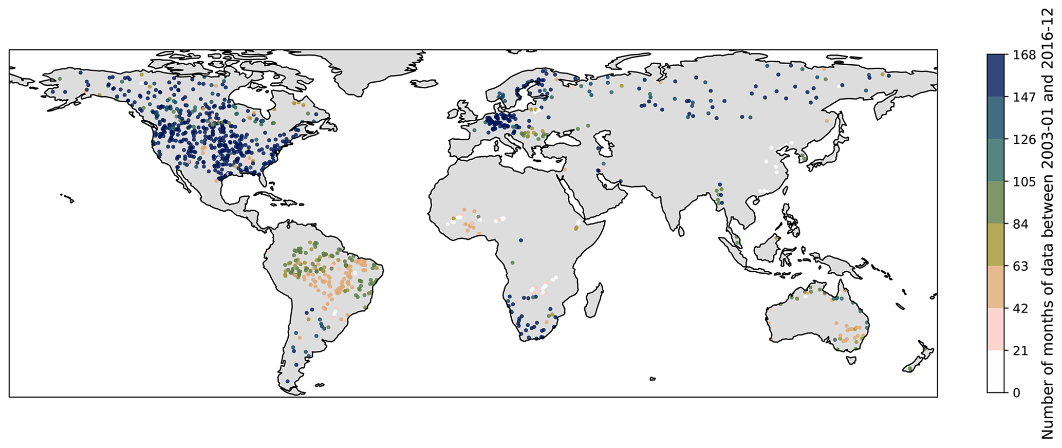
Figure 1 Locations of the acquired GRDC stations with runoff data.

Within the period 2003–2016, the selected stations have an average of 125 months of data, with just over half (515 stations) having more than 160 months of data out of a maximum possibility of 168 months. For the first 5 years of this period, nearly all the selected stations have data, with an average of 1015 data points being available each month. After 2008, the availability starts to decrease, and by 2008, the average number of data points per month drops to 580. A total of 143 117 monthly runoff records were used for the analysis.

Watershed boundaries were also obtained from the GRDC (GRDC, 2011). The largest catchment covers 4 680 000 km² (the Amazon River), and most of the catchments (862) are between 10 000 and 93 600 km². The mean catchment size is 141 259 km². Altitude was known for 764 of the stations, and the mean station altitude is 298.4 m a.s.l., with a large number (161) of stations being located at altitudes below 40 m a.s.l.

Many river basins contain multiple GRDC stations, meaning that, among the 1149 selected stations, some represent nested catchments.

The monthly mean GRDC data are given in cubic meters per second (m³ s⁻¹) and were converted to millimeters per month (mm month⁻¹) in order to be compared to the monthly runoff computed from remote sensing data. This was done by dividing by the catchment area.

2.3 Runoff time series from remote sensing

Solving the water balance for the different combinations of three precipitation, five actual evapotranspiration, and three storage change products results in a total of 45 solutions. Each of these solutions consists of a series of maps of the RS-derived runoff in millimeters per month (mm month⁻¹). For each GRDC station, the RS-derived runoff time series is obtained by averaging the pixels within the corresponding catchment.

Extracting these time series at the 1149 locations of the selected GRDC stations from these 45 combinations gives 51 705 time series to analyze.

In practice, the number of time series analyzed was lower due to several issues. First of all, calculated time series that have fewer than 30 matching data points with the GRDC data were omitted. Secondly, some of the selected stations (or their catchments) are (partially) located outside of the coverage area of some of the products (see Table 1). Finally, months for which more than 20 % of the pixels in a catchment were missing have been excluded (no gap filling has been done), occasionally leading to the loss of an entire times series (for example, as mentioned previously, SEBS has many missing pixels in some parts of the world). This finally resulted in 931 locations with sufficient data and 31 734 time series.

2.4 Validation

The computed monthly runoff time series have been compared with the GRDC data through the Nash–Sutcliffe efficiency (NSE) coefficient. The NSE is defined as follows (Nash and Sutcliffe, 1970):

$$\begin{array}{}\text{(3)}& \mathrm{NSE}=\mathrm{1}-{\displaystyle \frac{{\sum }_{t=\mathrm{1}}^T{\left({\mathrm{Ro}}_c^t-{\mathrm{Ro}}_{\mathrm{o}}^t\right)}^{\mathrm{2}}}{{\sum }_{t=\mathrm{1}}^T{\left({\mathrm{Ro}}_{\mathrm{o}}^t-\stackrel{\mathrm{‾}}{{\mathrm{Ro}}_{\mathrm{o}}}\right)}^{\mathrm{2}}}},\end{array}$$

where $\stackrel{\mathrm{‾}}{{\mathrm{Ro}}_{\mathrm{o}}}$ is the mean of the observed runoffs, ${\mathrm{Ro}}_c^t$ is the RS-derived runoff at time t, and ${\mathrm{Ro}}_{\mathrm{o}}^t$ is the observed runoff at time t.

2.5 Catchment characteristics

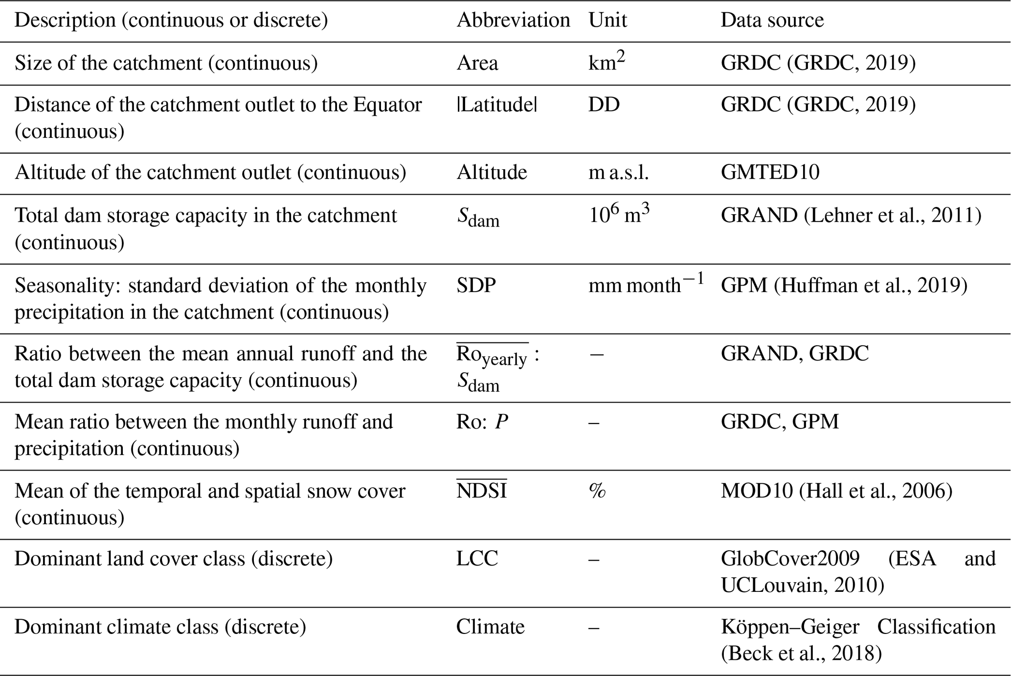
We selected 10 RS-derived catchment characteristics based on the findings of earlier studies to investigate correlations with the quality of RS estimates of discharge. These are summarized in Table 2 and detailed below.

Catchment area was chosen as a catchment parameter as it is expected that, in larger catchments, the random errors may be compensated for by averaging over large areas. Beyond this, the resolution of the GRACE product should also allow for better performance over larger catchments. While Biancamaria et al. (2019) found that GRACE could provide good estimates of storage change for catchments larger than 50 000 km², most studies have considered only very large basins (> 100 000 km²).

The latitude of the outlet of the catchment (or the distance to the Equator in degrees) and the snow cover were both chosen because precipitation products are known to have higher uncertainties at high latitudes and in the estimation of snow than in that of liquid precipitation (Tian and Peters-Lidard, 2010). Snow cover also adds a storage and therefore lag to the runoff generated in the basin which, while it should be captured by the GRACE data, can add another layer of uncertainty. ET products, in particular those based on measurements of land surface temperature, may also face issues in computing sublimation (Xu et al., 2019).

The altitude of the catchment outlet is evaluated to see any difference in accuracy between river catchments with an outlet at sea level and sub-catchments with an outlet at a higher altitude. The altitude of a catchment outlet is also used as a proxy for topography, and precipitation products are known to have higher uncertainty over areas of rough topography (Tian and Peters-Lidard, 2010).

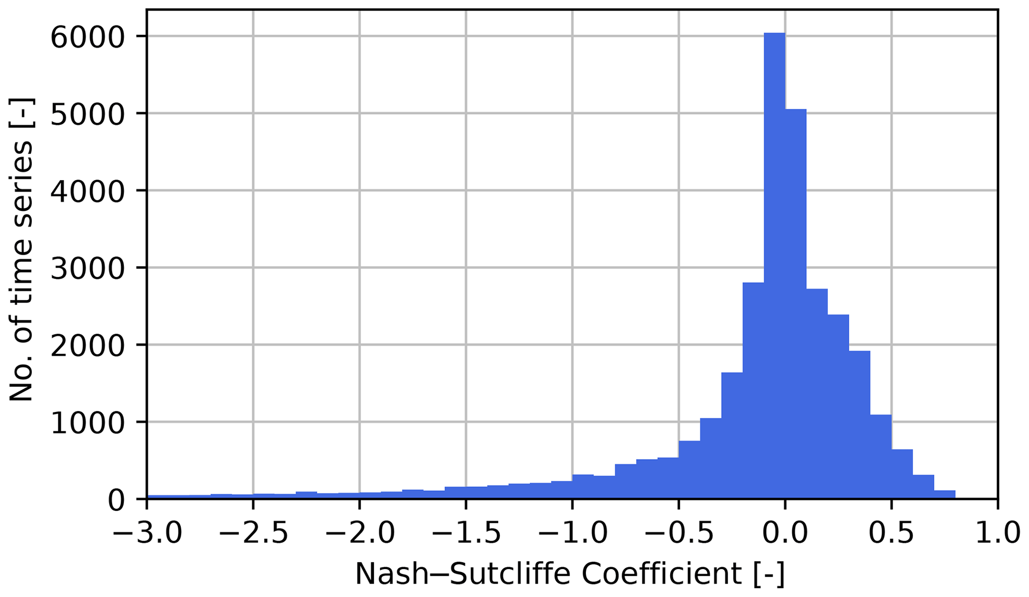
Figure 2 Distribution of NSE values for all time series; 891 time series with NSE < −3 not shown (2.8 % of time series).

Dam storage capacity was also considered due to the smoothing effect on the runoff. While the dam storage should be captured by the GRACE data, it has been shown that GRACE solutions do not always correctly locate the relatively punctual changes in dams' storage due to signal leakage which could impact the results (Wang et al., 2019). Dam storage capacity relative to mean annual runoff was also considered both as a measure of the level of modification of the basin and as normalization for total dam storage capacity.

The seasonality of rainfall varies greatly around the world. Some regions have a clear dry and wet season, while others receive rainfall throughout the entire year. In order to make a distinction between these different rainfall patterns, the standard deviation of the monthly rainfall was chosen as a parameter. A catchment with a clear wet and dry season will have a higher standard deviation than a catchment with precipitation throughout the year.

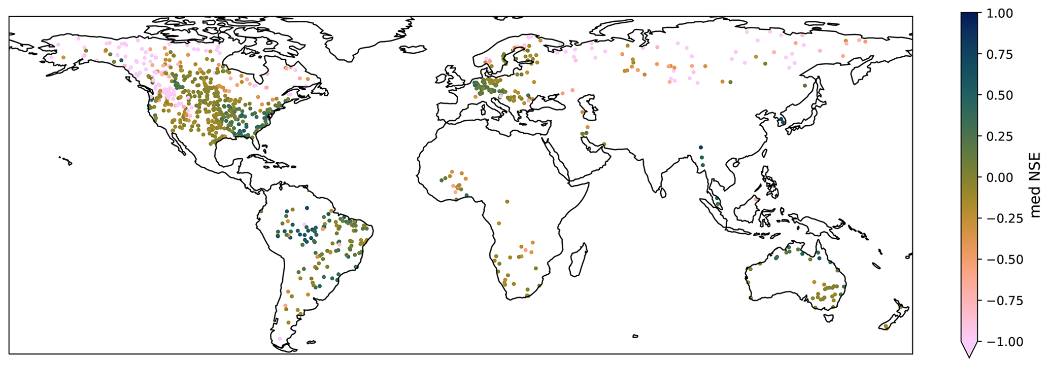
Figure 3 Median NSE for different product combinations at each GRDC station; 125 stations have a median NSE below −1. The color scale was cropped to −1 for legibility.

Finally, the ratio between runoff and precipitation is considered. Catchments with a low runoff-to-precipitation ratio will typically have a high evapotranspiration rate relative to precipitation, while a higher ratio indicates a low evapotranspiration rate. Catchments with ratios above 1 indicate discharge originating from either storage depletion in the basin or inter-basin transfers.

Besides the above characteristics which can be described by continuous variables, the following two discrete characteristics were considered.

The dominant climate class according to the Köppen–Geiger climate classification was computed for each catchment based on data from Beck et al. (2018). This was considered as previous water balance closure studies have shown variable performance under different climate conditions (e.g., Lorenz et al., 2014),

The final catchment characteristic considered was the dominant land cover class (LCC) in the catchment (computed from GlobCover2009 (ESA and UCLouvain, 2010)). This was considered due to the variable performance of ET products over different land cover types (e.g., Senay et al., 2013).

For each of the continuous catchment characteristics, the Spearman rank correlation coefficient, which is the Pearson correlation coefficient between the ranks of the variables, was computed to assess the correlation between each catchment characteristic and the NSE values of the discharge time series. The significance of the correlations (p<0.05) was tested using a two-sided Student's t test.

For the two non-continuous characteristics (LCC and climate class), the influence of the characteristics on the performance was analyzed by comparing the NSE values obtained per class.

3 Results and discussion

3.1 Results per GRDC station

NSE values were computed for the 45 possible product combinations for all GRDC stations possible for each combination. Figure 2 shows a histogram of the NSE values for all 31 734 time series computed, and Fig. 3 shows the median NSE values for all possible product combinations at each of the 931 GRDC stations for which at least one NSE value could be computed.

For all combinations of products at all available GRDC stations, 44.9 % of the generated discharge time series achieve a positive NSE value, with only 3.4 % obtaining an NSE > 0.5. When split by GRDC station, 36.9 % of the stations achieve a positive median NSE value, and 2.5 % achieve a median NSE of > 0.5. A positive NSE indicates that a model performs better than the long-term mean of the observed time series as a predictor. Hydrological models are often considered to be of good quality when reaching NSE values of > 0.5, although many studies use different thresholds (Moriasi et al., 2007).

When considering the maximum NSE reached at each station, it was determined that a positive NSE was reached for at least one product combination for 73.7 % of the stations, and an NSE of more than 0.5 was reached for 7.3 % of the stations. The geographical distribution of maximum NSE values is shown in Fig. 3.

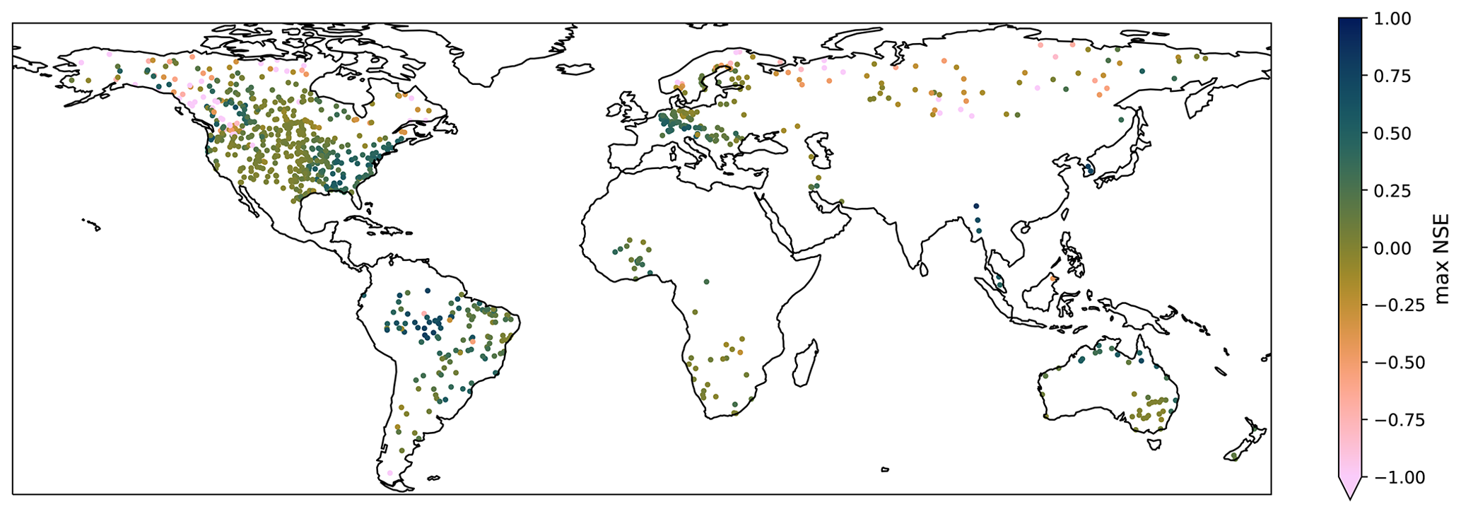
Figure 4 Max NSE achieved at each GRDC station; 43 stations have a maximum NSE below −1. The color scale was cropped to −1 for legibility.

In the studies performed by Lorenz et al. (2014), positive NSE values were reached in 29 of the 96 (30 %) basins considered, while in the study by Lehmann et al. (2022), this was achieved in 180 of 189 (95 %) of the basins. These results are, however, difficult to compare directly due to the different products chosen and the different basins considered. In terms of the datasets considered, we chose to limit our study to remote sensing products, excluding land surface models, station-based gridded products, and reanalysis products. This differs from the two aforementioned studies as our goal is to specifically investigate the remote sensing products and work with independent datasets.

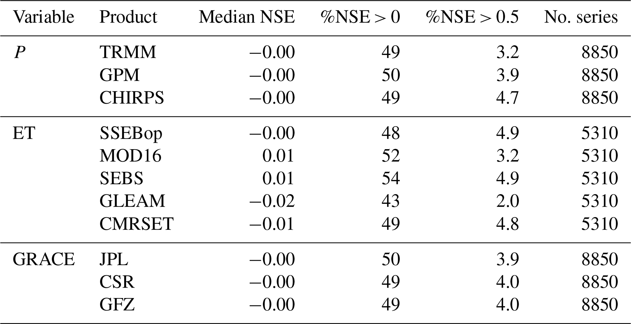
Table 3 Median NSE for time series containing specific products, as well as percentage of time series with positive NSE and NSE above 0.5 (n. NSE > 0.5) and the total number of time series using the product (n. series). Series have been limited to those covered by all product combinations (591 GRDC stations).

Our study, while it considers the largest number of catchments, was limited to those with GRDC station data available over our time period of interest, which excluded some large basins. On the other hand, many smaller catchments were considered, including nested catchments where multiple stations were available. Areas with more dense gauging networks are therefore overrepresented in our study, and these correlate with particular catchment characteristics (for instance, climate zone) which can influence the ability of remote sensing to close the water balance, as will be seen in Sect. 3.3.

3.2 Results per product and product combination

For the product combinations based on the GPM rainfall product, an average of 925 time series NSE values could be calculated per combination, while for the combinations based on the TRMM and CHIRPS products, an average of 599 NSE values per combination could be calculated (due to the smaller spatial coverage of TRMM and CHIRPS).

The median NSE values for all GRDC stations available for the 45 possible product combinations are presented in the Appendix A. The best-performing combination was CHIRPS–SEBS–JPL, which yielded 58 % of positive NSE values, while GPM–GLEAM–CSR/GFZ/JPL yielded 35 % of positive NSE values. Only 3.4 % of the discharge time series generated reached the threshold of 0.5, with the best combination (CHIRPS–CMRSET–GFZ) reaching this value for 5.9 % of stations. The worst-performing combination (GPM–GLEAM–GFZ) reached NSE > 0.5 for only 1.3 % of stations.

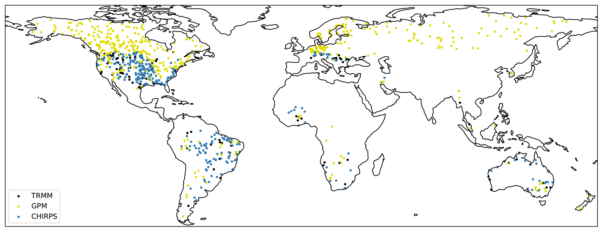
Figure 5 Precipitation product used in the combination with the highest NSE at each station. Note that GPM is the only product available for latitudes > 50^∘.

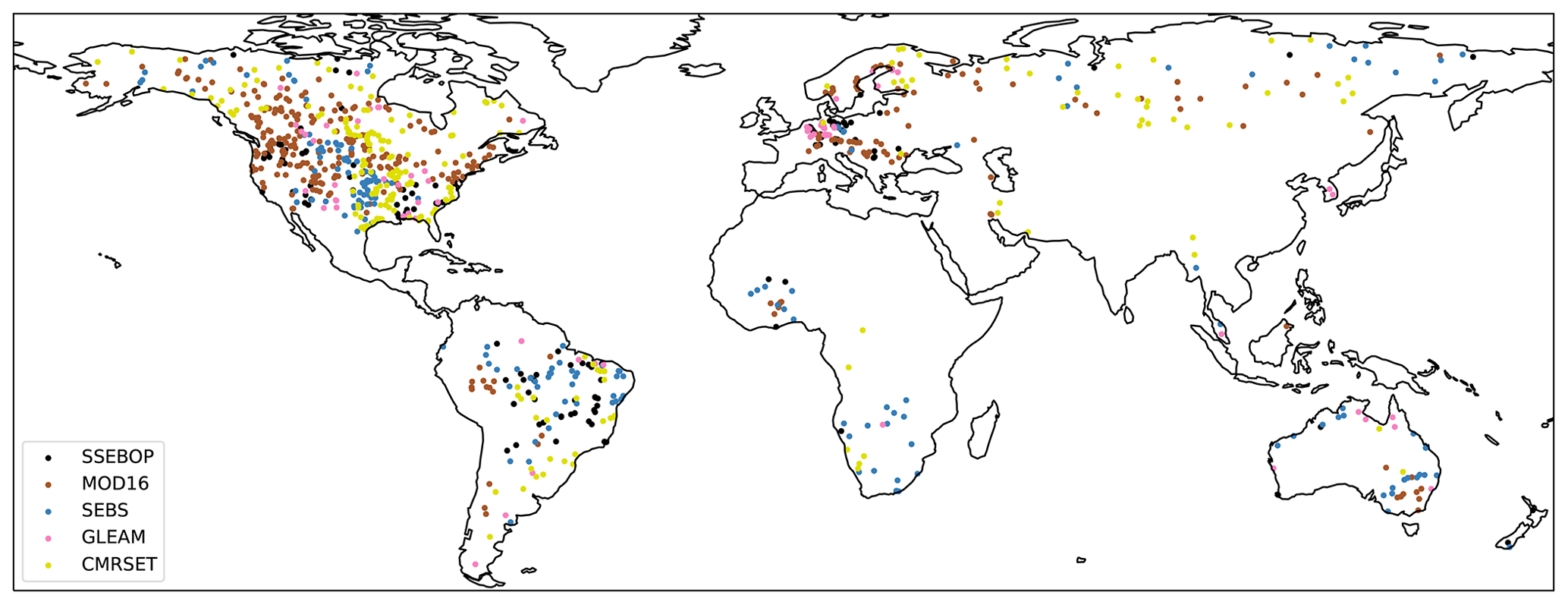
Figure 6 ET product used in the combination with the highest NSE at each station.

In order to make the product combinations more comparable, the same results are presented for (1) all possible time series (column A in Appendix A) and (2) only those stations for which all products could be used (column B in Appendix A). The main consequence of this is that the high-latitude stations which are only covered by GPM are removed from the analysis, which narrows the performance gap between GPM and other precipitation products.

Table 3 shows that the NSE of the computed discharge is most sensitive to the choice of ET product, with median NSE values ranging from −0.02 to 0.01. The ET product with the highest median NSE and number of NSE series with values above 0 is MOD16. The product with the highest number of series producing NSE values above 0.5 is SEBS (followed closely by SSEBop and CMRSET). For precipitation, the impact of different products on the overall median NSE is negligible when not considering high-latitude stations where only GPM is available. GPM produces the highest number of series with NSE values above 0, while CHIRPS produces the highest number of series with NSE values above 0.5. The computed NSE was not found to be sensitive to the choice of GRACE solution used.

The precipitation and ET products used in the best-performing combination for each station are shown in Figs. 4 and 5. Because of the low sensitivity of NSE to the storage change solution, no map was generated for the different storage change products.

These results show that no single product or combination consistently outperformed others when it comes to the closure of the water balance. This is consistent with findings of previous studies (Lehmann et al., 2022; Lorenz et al., 2014). Some geographic patterns in the better-performing products appear in Figs. 4 and 5 and will be discussed in the context of the catchment characteristics in the following section.

3.3 Results per catchment characteristic

For each of the continuous catchment characteristics listed in Table 2, correlations between the characteristic and the NSE at the GRDC station were computed. Figure 6 shows a summary of the correlations found for all product combinations and the catchment characteristics.

The presence or absence of correlation and the correlation strength and sign are consistent across most product combinations.

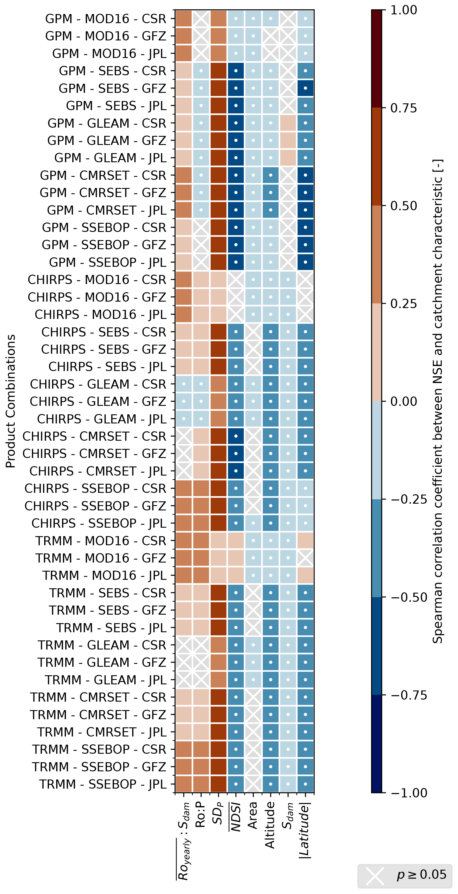
Figure 7 Spearman correlations for different product combinations between the NSEs of catchments and characteristics of those catchments. See Table 2 for an overview of the catchment characteristics. White dots were added to the negative correlations for monochromatic legibility.

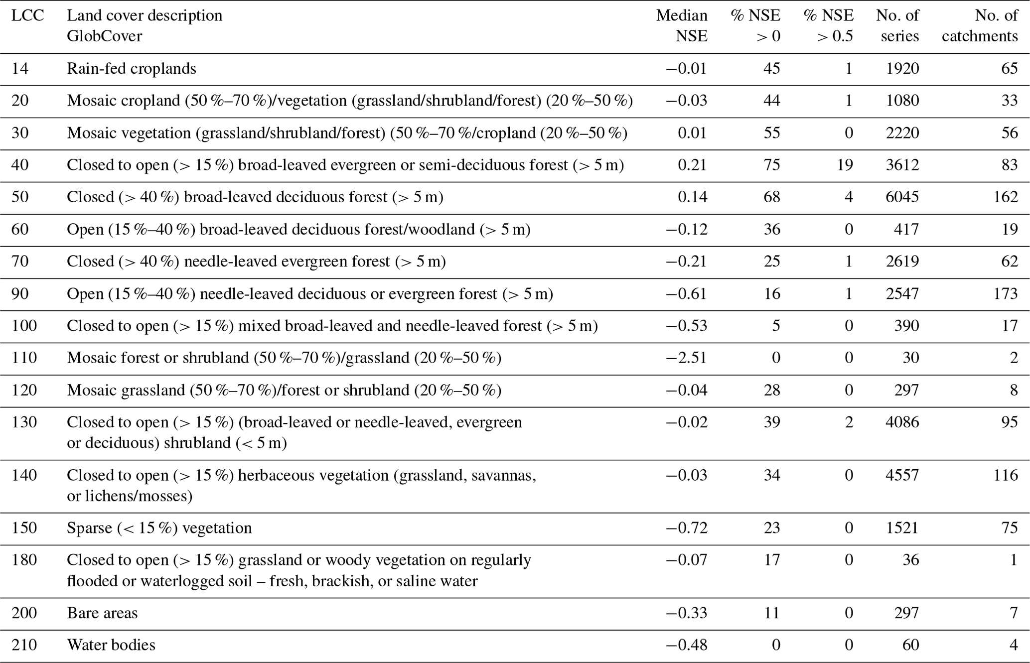
Table 4 NSE values for basins classified by dominant land cover class (LCC) and percentage of time series with positive NSE, percentage NSE above 0.5, and total number of time series with the corresponding land cover (no. of series) and the corresponding number of catchments (no. of catchments).

Of the catchment characteristics described by a continuous variable, seasonality (SDp) shows the strongest correlation with the NSE of the discharge. All product combinations showed a significant correlation with the standard deviation of precipitation. It should be noted that precipitation from GPM was used to compute seasonality, meaning that errors and uncertainties in GPM data could affect catchment classification. The influence of seasonality is in agreement with the findings of Lorenz et al. (2014), who found that the closure of the water balance can be better achieved in basins with a strong seasonal precipitation signal. Lorenz et al. (2014) observed that, in catchments with low seasonal runoff variability, the biases in the different input datasets prevented the accurate computation of runoff.

Snow cover has the strongest negative correlation with NSE. The mean normalized difference snow index ($\stackrel{\mathrm{‾}}{\mathrm{NDSI}}$) shows a significant negative correlation for 39 of the 45 product combinations. Combinations including MODIS ET and CHIRPS or TRMM precipitation are the only ones for which no correlation or a positive correlation was found. Altitude at the gauging station, which is correlated to snow cover for smaller basins, shows a weaker negative correlation with NSE. The strong negative correlation with snow could be due to multiple factors. For instance, snow retrievals have lower accuracies as compared to liquid precipitation retrievals from satellites, and precipitation retrievals are less accurate over frozen ground (Tang et al., 2020; Tian et al., 2014; Tian and Peters-Lidard, 2010); ET products may not capture the process of sublimation as well as other types of ET (see, e.g., Xu et al., 2019), and the snow storage variations which drive discharge timing in some catchments may not be adequately captured by GRACE. Analysis of runoff versus discharge totals over hydrological years rather than monthly could mitigate the snow storage issue. A similar analysis with more recent data should also be carried out to check if better results for catchments further from the Equator (> 50^∘ N and > 50^∘ S) can be obtained as the GPM data from the TRMM era (pre-2014) for higher latitudes are considered to constitute partial coverage. The GPM core observatory also has higher sensitivity to snowfall than earlier sensors (Behrangi et al., 2018) and was only launched in 2014.

Latitude also shows a correlation with NSE for 39 out of 45 product combinations, while the remaining 6 show the same pattern as for snow cover. This negative correlation was expected based on the more extensive snow cover and frozen ground found further from the Equator, which negatively impacts performance for both P and ET products, as explained above. GRACE measurements are also subject to the effects of the glacial isostatic adjustment (GIA), the redistribution of mass within the Earth resulting from the end of the last ice age (Wahr et al., 1998). While the GIA signal is removed from GRACE TWSA data products, any errors in the GIA models used in this process will result in higher errors in TWSA where the GIA signal is strongest, which correlates with higher latitudes.

Dam storage capacity shows a negative correlation with NSE only for product combinations using GPM as a precipitation product and for the TRMM–MOD16 combination. For other combinations, no significant correlations were found. Total runoff relative to dam storage capacity shows a negative correlation for most product combinations, except for CHIRPS–GLEAM (positive) and TRMM–GLEAM (no significant correlation).

Runoff ratio shows a negative correlation with NSE for 12 out of the 45 combinations and a positive correlation for 24 out of the 45. Runoff ratio is computed as the ratio of discharge from GRDC and precipitation from GPM, and the maximum value found was 42, indicating potentially erroneous data or a strong proportion of discharge originating from storage depletion or inter-basin transfers. Inter-basin transfers in particular would not be represented in our computation of runoff. The runoff ratio was found to be above 1 for 103 stations (out of 931).

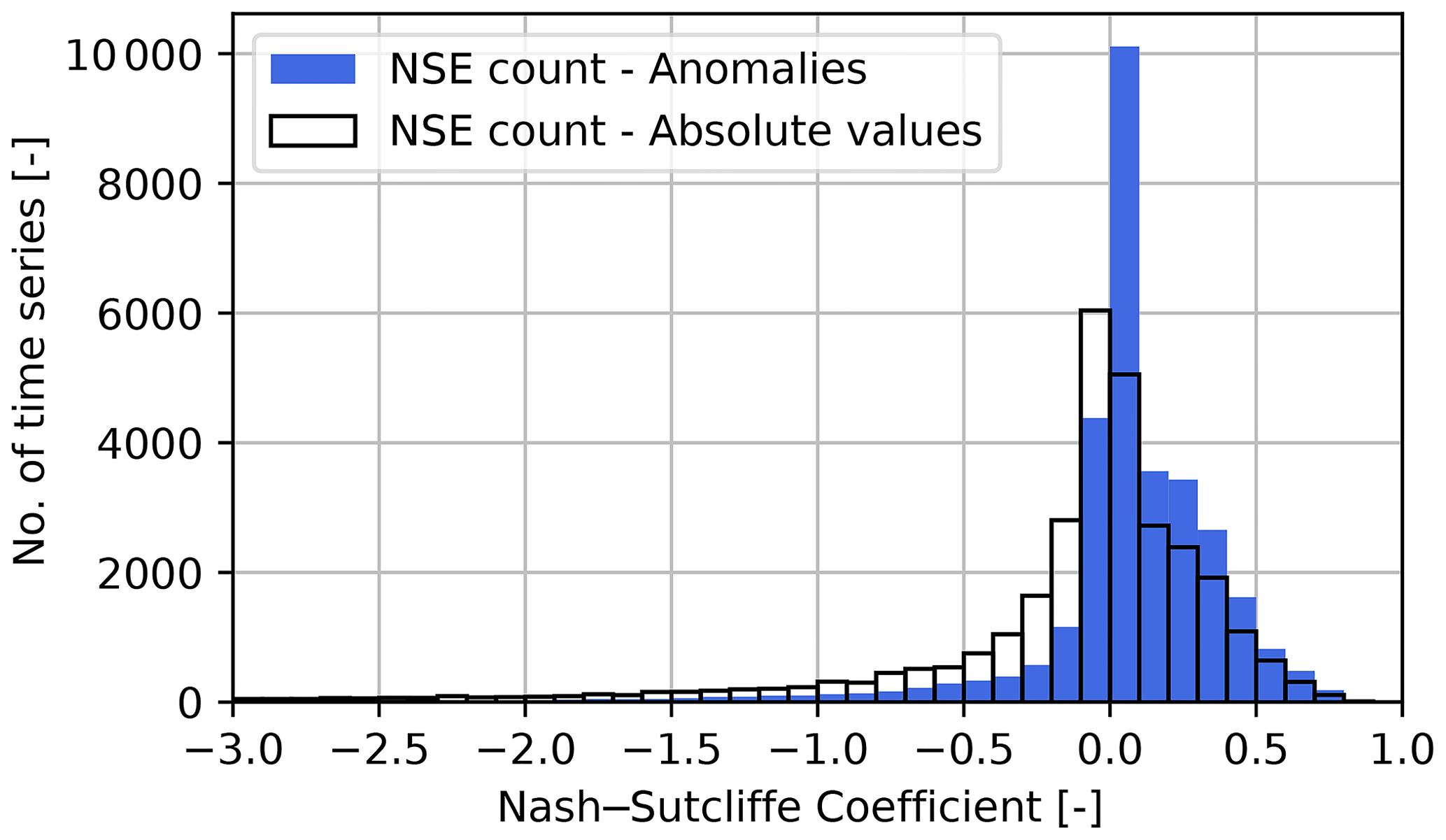
Figure 8 Distribution of NSE values for all time series for the standard and anomaly time series. Time series with NSE < −3 not shown – 2.8 % of time series for standard and 0.7 % for the anomaly time-series.

A weak negative correlation was found between drainage area and the NSE of the RS-derived runoff for 28 of the combinations. The lack of a strong correlation between NSE and catchment area is surprising as the storage change component from GRACE is expected to perform better over larger catchments, particularly because we limited the catchment size here to catchments larger than 10 000 km², while GRACE has an inherent spatial resolution of ∼ 300 km (90 000 km²) and has been found to produce reliable estimates of storage change for catchments with areas of more than 50 000 km² (Biancamaria et al., 2019). Smaller catchments will also be more susceptible to signal leakage from outside the catchment (Dutt Vishwakarma et al., 2016). Catchment size is also expected to influence the applicability of the hypothesis of negligible subsurface fluxes, which is necessary for the application of Eq. (2), as this hypothesis has been shown to be incorrect for smaller catchments (Bouaziz et al., 2018; Fan and Schaller, 2009). Sahoo et al. (2011) and Lehmann et al. (2022) similarly found no correlation between basin area and water balance closure, though their studies were limited to 10 very large basins and basins with areas larger than 65 000 km², respectively.

Table 5 Median NSE values per product and per dominant LCC. Cells in italic bold have median values > 0, and cells in bold have values > 0.1. Empty cells represent a category where a specific product is not available.

Table 6 NSE values for basins classified by climate class.

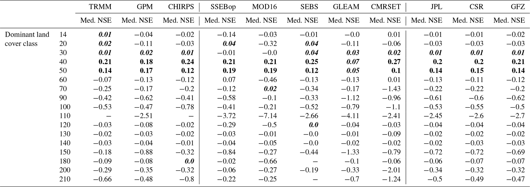
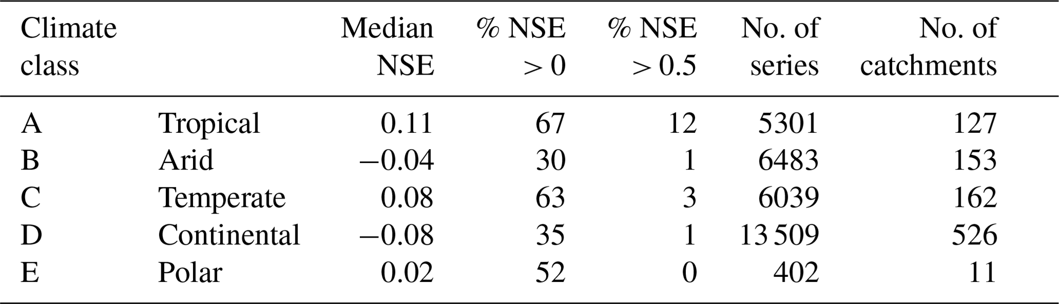
Table 7 Median NSE values per product and dominant climate class. Cells in italic bold have median values > 0, and cells in bold have values > 0.1.

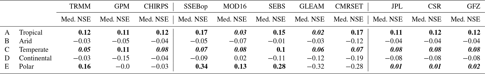
Figure 9 Median NSE for the anomaly time series for different product combinations at each GRDC station; 49 stations have a median NSE of below −1. The color scale was cropped for legibility.

Results for the two discrete variables (dominant land cover type and dominant climate class) are shown in Tables 4, 5, 6, and 7.

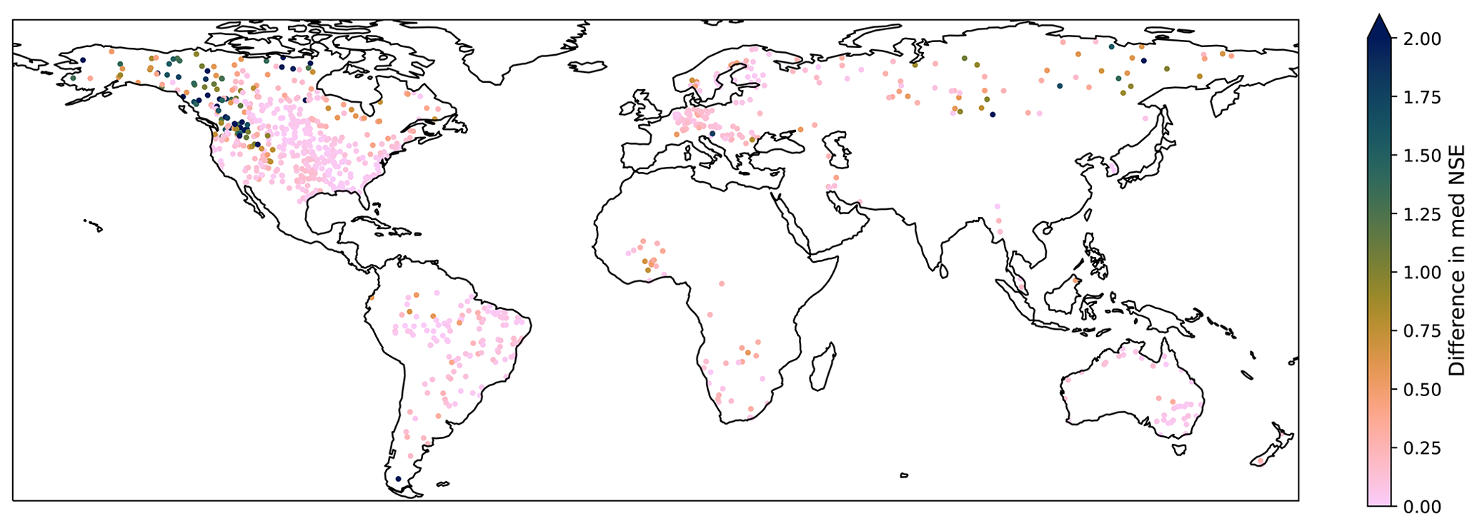
Figure 10 Difference in median NSE values between anomaly and original time series. Positive values denote an increase in NSE for anomaly time series – all stations saw an increase in median NSE by moving to the anomaly; 26 stations saw an increase of more than 2. The color scale was cropped for legibility.

Variability was found between the results for different land cover types. Results for basins with dominant land cover codes 40 and 50 (both types of broad-leaved forests; see Table 4) perform better than other land cover types, with median NSE values of 0.21 and 0.14, respectively.

Some land cover classes, for example open (15 %–40 %) needle-leaved deciduous or evergreen forest (> 5 m) (class 90), perform particularly poorly, which can be expected as these have a near-complete overlap with higher-latitude areas. MOD16 performs better than other products in this land cover class, with a median NSE value of −0.1, while combinations using the other ET products produce median NSE values between −0.33 and −0.96 (Table 5).

Variability is also observed between climate zones, with tropical (median NSE = 0.11 and median NSE for tropical monsoon of 0.28; see Table 6 and Appendix A for the detailed results per climate zone) and temperate zones (median NSE = 0.08) performing better than arid (median NSE = −0.04) and continental zones (median NSE = −0.08). The SSEBop and CMRSET products produce the highest NSE values in tropical climates, with median NSE values of 0.17, followed by SEBS at 0.15 (Table 7). In temperate zones, using GPM produces the highest median NSE values of 0.11. Lehmann et al. (2022) also analyzed the water balance closure by climate zone and found that errors were relatively consistent within zones, with some exceptions. As in this study, the best performance was observed in the equatorial rain forest/monsoon zone. This result is also in agreement with the influence of seasonality of rainfall discussed above and observed by Lorenz et al. (2014). Sahoo et al. (2011), on the other, hand did not find consistent behavior based on climate zone.

3.4 Results considering anomalies

Remote sensing products are known to be subject to biases, and in the results presented so far, no bias correction was considered. In order to investigate how biases may impact the results, we computed the NSE using the anomalies from the mean of the computed runoff and GRDC data. The anomalies from the mean were computed by subtracting the mean of each time series from the time series values.

Considering anomalies rather than absolute values produces a shift in the distribution of the computed NSE values towards higher values (Fig. 8), with the percentage of time series reaching NSE > 0, going from 44.9 % to 72.1 %, and the percentage of time series reaching NSE > 0.5, going from 3.4 % to 4.8 %.

Increases in NSE for the anomaly time series are most pronounced in the areas which had very low NSE values (see Figs. 3 and 10), but many of these retain low NSE values, as can be seen, for example, in the northwestern Americas in Fig. 9.

Results in terms of the correlation of NSE with catchment characteristics show some differences in the magnitude of the correlations but very few in the sign of the correlation, with the notable exception of the correlations between runoff-to-precipitation ratios for GPM products. We therefore expect that, while using NSE for the anomalies from the mean may show some differences, the general conclusions would be similar to those presented for the standard time series. The table of correlations for the anomaly time series is shown in Appendix B.

4 Conclusions and perspectives

In this study, we analyzed the closure of the water balance at the monthly timescale for catchments of more than 10 000 km² by using remote sensing to compute runoff and by comparing the computed runoff to in situ measurements of discharge from the GRDC using the Nash–Sutcliffe efficiency as the performance metric. We computed the results for 45 different remote sensing product combinations at between 595 and 931 gauging stations, depending on the product combinations, and we analyzed the results through the lens of both the remote sensing products and 10 catchment characteristics which we computed globally.

Overall, a positive NSE could be reached for at least one product combination for 73.7 % of the stations considered. While some product combinations showed better results than others, no one combination or product stood out as systematically performing better than the others. Correlations were found between the NSE values obtained and the ability of remote sensing to close the water balance between areas with different precipitation patterns, in areas with large snow cover, in different climatic zones, and in areas with different dominant land cover classes. This highlights the importance of validating RS products widely. In particular, our results point to the necessity of the improvement of products in continental and arid climate zones and some land covers.

While a number of catchment characteristics were analyzed, these are not exhaustive, and those chosen could have also been computed differently. For example, for larger basins, selecting only one land use category as representative can obscure some differences, and using percentages of area under different types of vegetation may help to further refine results. The same may be considered for climate class. An additional characteristic which could be interesting to investigate is the percentage of area under irrigation, particularly for potentially differentiating the different ET products and as a measure of the degree of alteration. One limitation of such an analysis would be the accuracy of global irrigation maps. Some examples of other catchment characteristics which suffer from similar limitations in terms of global data availability or quality but would be of interest are soil type and hydrogeology.

Many satellite products are also calibrated in specific areas, though it is not always straightforward to obtain this information consistently. It would be very interesting to assess how different the performance is in areas where calibration activities are carried out versus others and how this impacts the choice of product. These areas may also be correlated with areas with a high density of GRDC stations. Efforts to collect discharge data in underrepresented areas should be undertaken to be included in future studies.

Appendix A: Full result tables for all combinations and by climate zone

Table A1 Median NSE values for the 45 product combinations. No. of NSE > x is the number of time series for which NSE > x, and no. of catchments is the number of series considered for the specific combination (one per catchment). The results are presented both for all GRDC stations available for each combination (A) and for the GRDC stations common to all product combinations (B).

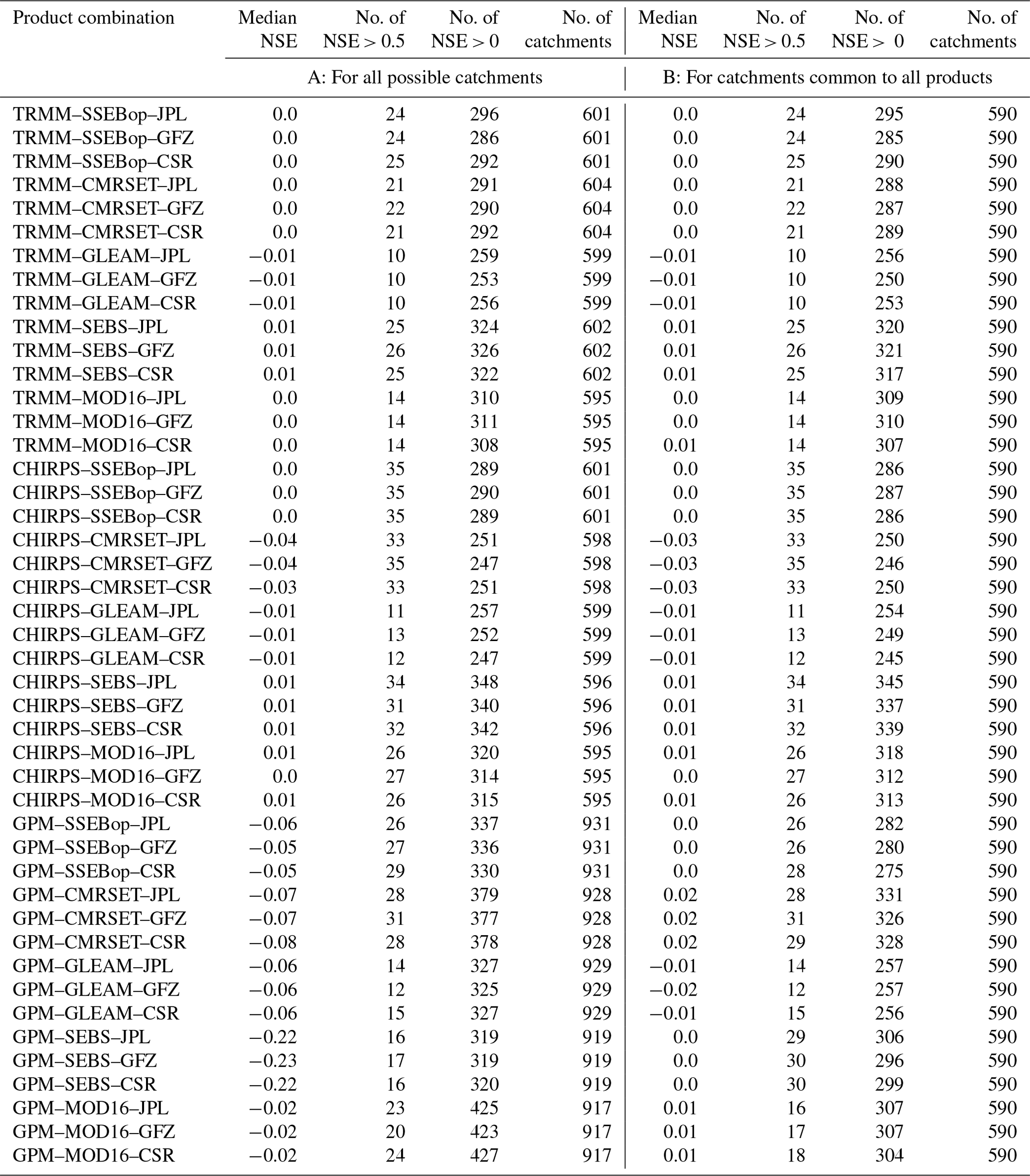
Table A2 Full results by climate zone – % NSE > x is the percentage of time series for which NSE > x, no. of series is the number of time series produced for each climate class, and no. of catchments is the number of catchments located in the different climate classes.

Appendix B: Correlation table for anomaly time series

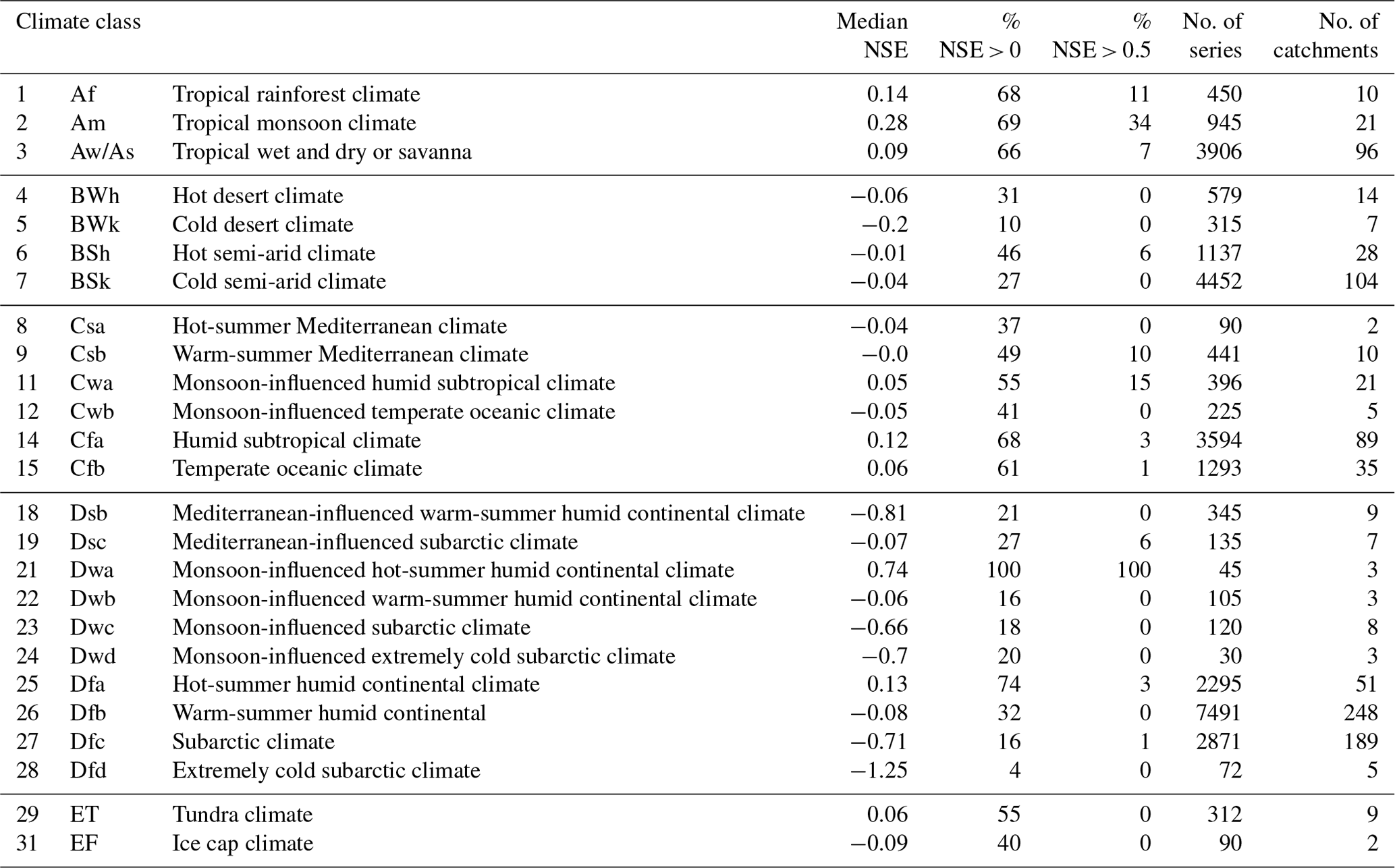
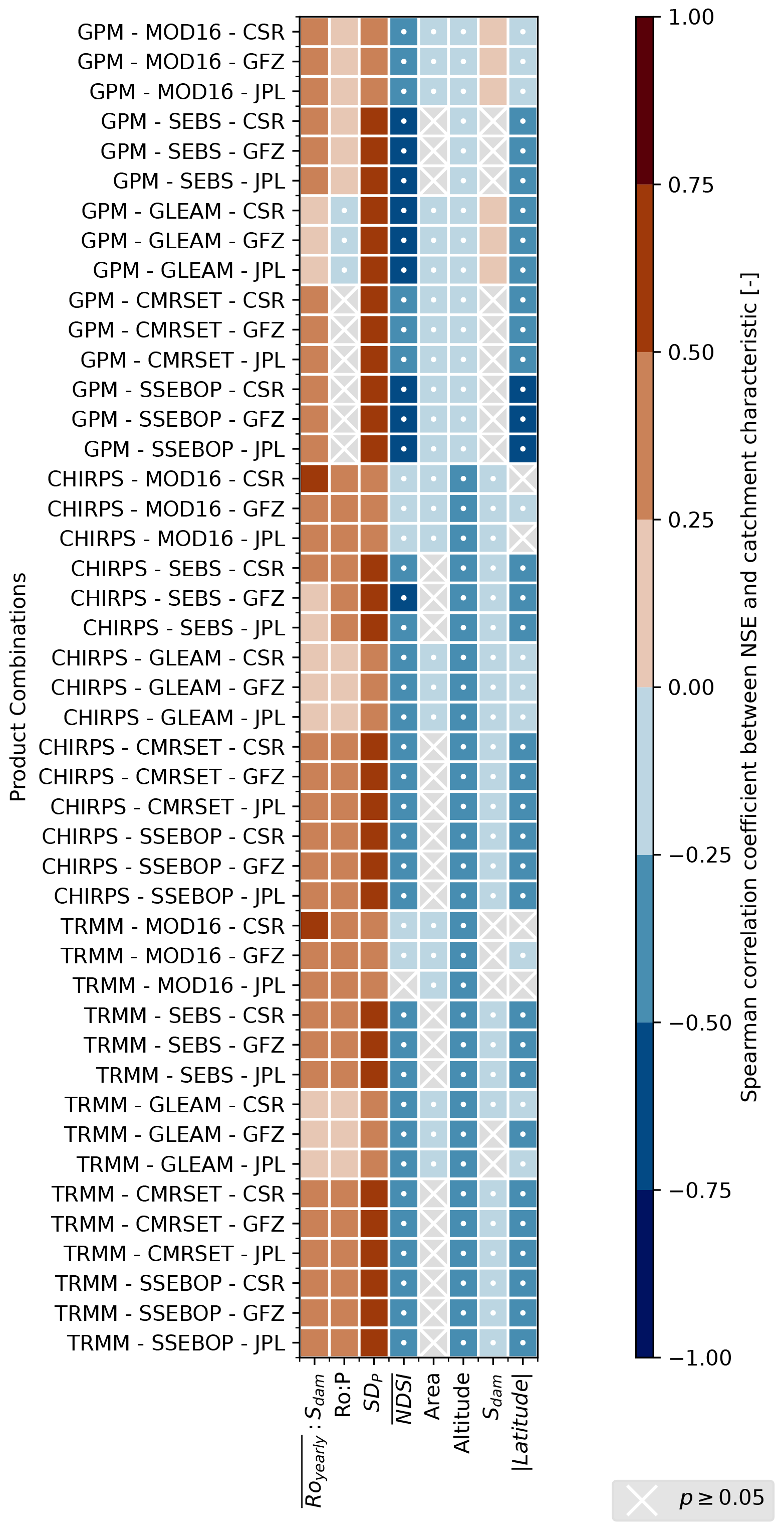
Figure B1 Spearman correlations for different product combinations between the NSEs of anomaly time series for catchments and characteristics of those catchments. See Table 2 for an overview of the catchment characteristics. White dots were added to the negative correlations for monochromatic legibility.