the Creative Commons Attribution 4.0 License.
the Creative Commons Attribution 4.0 License.
 | 19 Jan 2023
Numerical assessment of morphological and hydraulic properties of moss, lichen and peat from a permafrost peatland
Simon Cazaurang
Manuel Marcoux
Oleg S. Pokrovsky
Sergey V. Loiko
Artem G. Lim
Stéphane Audry
Liudmila S. Shirokova
Laurent Orgogozo
Due to its insulating and draining role, assessing ground vegetation cover properties is important for high-resolution hydrological modeling of permafrost regions. In this study, morphological and effective hydraulic properties of Western Siberian Lowland ground vegetation samples (lichens, Sphagnum mosses, peat) are numerically studied based on tomography scans. Porosity is estimated through a void voxels counting algorithm, showing the existence of representative elementary volumes (REVs) of porosity for most samples. Then, two methods are used to estimate hydraulic conductivity depending on the sample's homogeneity. For homogeneous samples, direct numerical simulations of a single-phase flow are performed, leading to a definition of hydraulic conductivity related to a REV, which is larger than those obtained for porosity. For heterogeneous samples, no adequate REV may be defined. To bypass this issue, a pore network representation is created from computerized scans. Morphological and hydraulic properties are then estimated through this simplified representation. Both methods converged on similar results for porosity. Some discrepancies are observed for a specific surface area. Hydraulic conductivity fluctuates by 2 orders of magnitude, depending on the method used.
Porosity values are in line with previous values found in the literature, showing that arctic cryptogamic cover can be considered an open and well-connected porous medium (over 99 % of overall porosity is open porosity). Meanwhile, digitally estimated hydraulic conductivity is higher compared to previously obtained results based on field and laboratory experiments. However, the uncertainty is less than in experimental studies available in the literature. Therefore, biological and sampling artifacts are predominant over numerical biases. This could be related to compressibility effects occurring during field or laboratory measurements. These numerical methods lay a solid foundation for interpreting the homogeneity of any type of sample and processing some quantitative properties' assessment, either with image processing or with a pore network model. The main observed limitation is the input data quality (e.g., the tomographic scans' resolution) and its pre-processing scheme. Thus, some supplementary studies are compulsory for assessing syn-sampling and syn-measurement perturbations in experimentally estimated, effective hydraulic properties of such a biological porous medium.
- Article
(4979 KB) - Full-text XML
-
Supplement
(15263 KB) - BibTeX
- EndNote


Covering a quarter of the Northern Hemisphere's land surface (Brown et al., 1997), permafrost soils are the most representative soil types in arctic and subarctic regions. Permafrost is a soil layer in which temperature remains below 0 ∘C for at least 2 consecutive years, thus holding ice in its porous structure. Frozen layers make permafrost hydrology peculiar, resulting in complex couplings between heat and water fluxes (Grenier et al., 2018; Tananev et al., 2020). Seasonal structural variations occur in permafrost soils, as surface thawing forms an “active layer”. Most permafrost-related biogeochemical processes (especially organic matter degradation) take place in this layer. The active layer is at its maximum thickness in the early fall and is generally meters in scale (Clayton et al., 2021; Aalto et al., 2018; Guo and Wang, 2017). Active layer thickness is, nonetheless, spatially variable due to climatic conditions, land cover, and the micro- and macro-topography. The impact of hydrological climate change is particularly drastic in permafrost-dominated environments because of deepening thaw fronts (Hinzman and Kane, 1992). Indeed, between 2008 and 2016, the average annual temperature of arctic permafrost soil increased by 0.4 (±0.25) ∘C (Biskaborn et al., 2019; Fox-Kemper et al., 2023). This causes positive feedback on average atmospheric temperatures (Meredith et al., 2019), reduces latent heat effects (Walwoord and Kurylyk, 2016) and increases water drainage in arctic watersheds (Liljedahl et al., 2016). Hence, quantifying heat and water transfer properties in permafrost-affected regions is compulsory.
Previous studies have addressed this quantification through field observations (Olefeldt and Roulet, 2014; Streletskiy et al., 2015; Throckmorton et al., 2016; O'Connor et al., 2020) or field and laboratory experiments (Vedie et al., 2011; Roux et al., 2017; Wagner et al., 2018). Some recent studies have also dealt with this question using a modeling approach (Bense et al., 2012; Genxu et al., 2017; Burke et al., 2020; Du et al., 2020; Fabre et al., 2017).
Bryophytes (mosses) and lichens are widely present in tundra and taiga environments. The dominant ground cover consists of Sphagnum mosses and lichens in permafrost peatlands (Soudzilovskaia et al., 2013; Volkova et al., 2018). Sphagnum mosses are part of the Bryophyta plant division, which represents non-vascular plants (without xylem or phloem). Sphagnum colonies grow indeterminately from their apical structure, named the capitula. Their water content mainly relies on capillary forces maintained by each individual's density (Hayward and Clymo, 1982; Howie and Hebda, 2018). Lichens are not “vegetation” but consist of a symbiotic association between heterotrophic Fungi and autotrophic Algae. Both Sphagnum and lichens can be gathered into the Cryptogamae subkingdom. This cryptogamic layer has an important impact on permafrost dynamics because it influences heat and water exchanges between the soil and atmosphere (Soudzilovskaia et al., 2013; Launiainen et al., 2015; Porada et al., 2016; Park et al., 2018; Loranty et al., 2018). Boreal vegetation is assumed to be a major nutrient and inorganic solute exchange medium at a watershed scale (Shirokova et al., 2021). Boreal vegetation is likely to accumulate in lowlands at a low degradation rate, resulting in the formation of Sphagnum peatlands, such as the Western Siberian Lowlands.
Ground vegetation transfer properties are key information for high-resolution hydrological modeling of permafrost-related catchments. Thus, reliable estimates of them are necessary for water flux studies for boreal soils and for climate change impact assessment of the hydrology of high-latitude continental surfaces. Therefore, some recent efforts have been put into emphasizing the role of the cryptogamic layer in Earth system models (Stepanenko et al., 2020; Shi et al., 2021). Devoted modeling tools have also been created to predict Sphagnum dynamics (the Peatland Moss Simulator by Gong et al., 2020). Furthermore, specific modeling work has been conducted on restored Sphagnum peatlands to link hydrological properties with dissolved organic carbon dynamics (Bernard-Jannin et al., 2018) or soil moisture dynamics (Elliott and Price, 2020). However, the mechanistic modeling of water and heat fluxes in ground vegetation layers remains difficult, as their porous-medium transfer properties are not straightforward to evaluate (Orgogozo et al., 2019).
Many studies are available for the decayed Sphagnum layer: peat. The hydrological and thermal properties of peat are well documented. Extensive reviews of the relation between hydrogeochemical processes in peatlands and peat's porous-medium structure were conducted by McCarter et al. (2020). A study of peatland's hydraulic properties was initiated during the 1920s for peatland drainage (Malmström, 1925). Then, some introductory field experiments were conducted on Finnish peatlands (Virta, 1962; Heikurainen, 1963; Sarasto, 1963) as well as in the United States (Boelter, 1968) and Ireland (Galvin, 1976).
Only a few studies were conducted on the living part of this upper permafrost layer. Hence, quantitative assessments of some key hydrological properties of ground vegetation layers are needed, such as total, open and enclosed porosity, hydraulic conductivity and specific surface area. In terms of hydraulic properties, hydraulic conductivity has been assessed in the laboratory using constant or falling-head permeameters (Quinton et al., 2000; Price et al., 2008; Hamamoto et al., 2016; Weber et al., 2017) or via field measurements (Päivänen, 1973; Crockett et al., 2016; this study). The results are presented in Table 2, with some peat results for comparison. Otherwise, arctic lichens have received little attention to date. To our knowledge, only one study has estimated lichens' hydraulic properties, considering unsaturated hydraulic conductivity without taking into account macropores (Voortman et al., 2014). However, the specific surface areas of some other lichen species are documented in the literature (Adamo et al., 2007). Some studies quantified arctic lichen properties in response to acid rain (Tarhanen et al., 1999) to clarify their interaction with the rhizosphere (Banfield et al., 1999) or in relation to their albedo properties (Bernier et al., 2011). Some transmembrane transfer properties are also available in the literature (Potkay et al., 2020)
Table 2Synthesis of saturated hydraulic conductivity (m s−1) of peat and Sphagnum found in the literature. This study's values refer to field experiments conducted during sample collection (CHP: constant head permeameter; FHP: falling head permeameter; FP: field percolation; IM: inverse modeling; NM: numerical model, Hydrus-1D; see McCarter and Price, 2012).
Thus, many field and experimental studies are available throughout the literature. However, field work and experimental studies are known to bring their own difficulties, due to the local conditions' variabilities, sampling biases, disturbances and measurement uncertainties. The aim of this study is to assess some of the transfer properties that are well documented with field and experimental studies with an innovative numerical scheme. Indeed, the use of numerical workflows enhances reproducibility and intercomparison capability between samples. Numerical workflows are often used when experimental studies are complicated to implement (reservoir engineering, aerodynamics, micro-fluidics).
In this work, such numerical workflow is intended to be used for evaluating the hydrological transfer properties of representative vegetation types of the Western Siberian Lowlands. To this end, natural samples collected from the Western Siberian Lowlands are digitally analyzed to characterize some morphological and hydraulic transfer properties. Thus, in contrast to previous works compiled in Table 2, this study aims to assess the hydraulic properties of lichens and Sphagnum mosses by numerical methods rather than experimental measurements. The arctic cryptogamic layer is assumed, hereafter, to represent a complex patchwork of biological porous media (Price et al., 2008, Voortman et al., 2014, Hamamoto et al., 2015).
To validate this hypothesis, a thorough analysis of sample homogeneity is carried out, based on porosity, as it is the main driver of flow dynamics in porous media (Koponen et al., 1996, 1997). This enables the classification of samples according to their homogeneity. Indeed, for homogeneous samples, a smaller sample region can be considered an effective medium sharing the same properties as the whole sample. Multidimensional porosity description leads to a statistical study of the existence of a representative elementary volume (REV). Two standard porous-medium modeling methodologies are used throughout this study: direct numerical simulations on computed representative elementary volumes (DNS-REVs) and pore network modeling with a built-in solver (PNM). The impossibility of collecting a substantial number of samples is compensated for by a statistical quantification of a REV for each sample. This implies that the REV is smaller than the sample, and hence sampling size is chosen to match sizes that were used in the previous literature, such as Weber et al. (2017).
2.1 Sample collection and digital reconstruction
Samples were collected at Khanymei Research Station (N63∘43′19,73′′ E75∘57′47,91′′) in Western Siberia (Autonomous District of Yamal-Nenets, Russian Federation) in July 2018. The mean annual temperature is −5.6 ∘C, and average precipitation is 540 mm (Payandi-Rolland et al., 2020; Raudina et al., 2018). Eight moss samples (Sphagnum sp.) were collected, either on moss mounds or in thermokarstic hollows. Additionally, two lichen samples (Cladonia sp., named Lichen1.3 and Lichen2.1) and two peat samples (named Peat2.2 and Peat2.3) were collected. Of the eight Sphagnum samples, three are S. angustifolium (C.E.O. Jensen ex Russow, named Mound2.4, Mound2.5 and Mound2.6), two are S. lindbergii Schimp (named Hollow1.2 and Hollow1.4) and two are S. majus (Russow) (C.E.O. Jensen, named Hollow2.7 and Hollow2.8). The last moss sample is S. lenense H. Lindb. ex L.I. Savicz (named Mound1.1).
Sampling is thoroughly conducted to minimize structural perturbations. In order to achieve this, each sample's surroundings are cleared with special care prior to extraction. Then, the sample is extracted using a ceramic knife directly at the right dimensions to fit in a high-density polyethylene box, where it remains from the moment of sampling and drying to the tomographic examination. Additionally, four in situ hydraulic conductivity measurements are performed on various Sphagnum plots, using a double-ring infiltrometer (Table 2). An overview of the sample collection method is shown in Fig. 1 as well as 3D tomographical visualizations of each sample type.
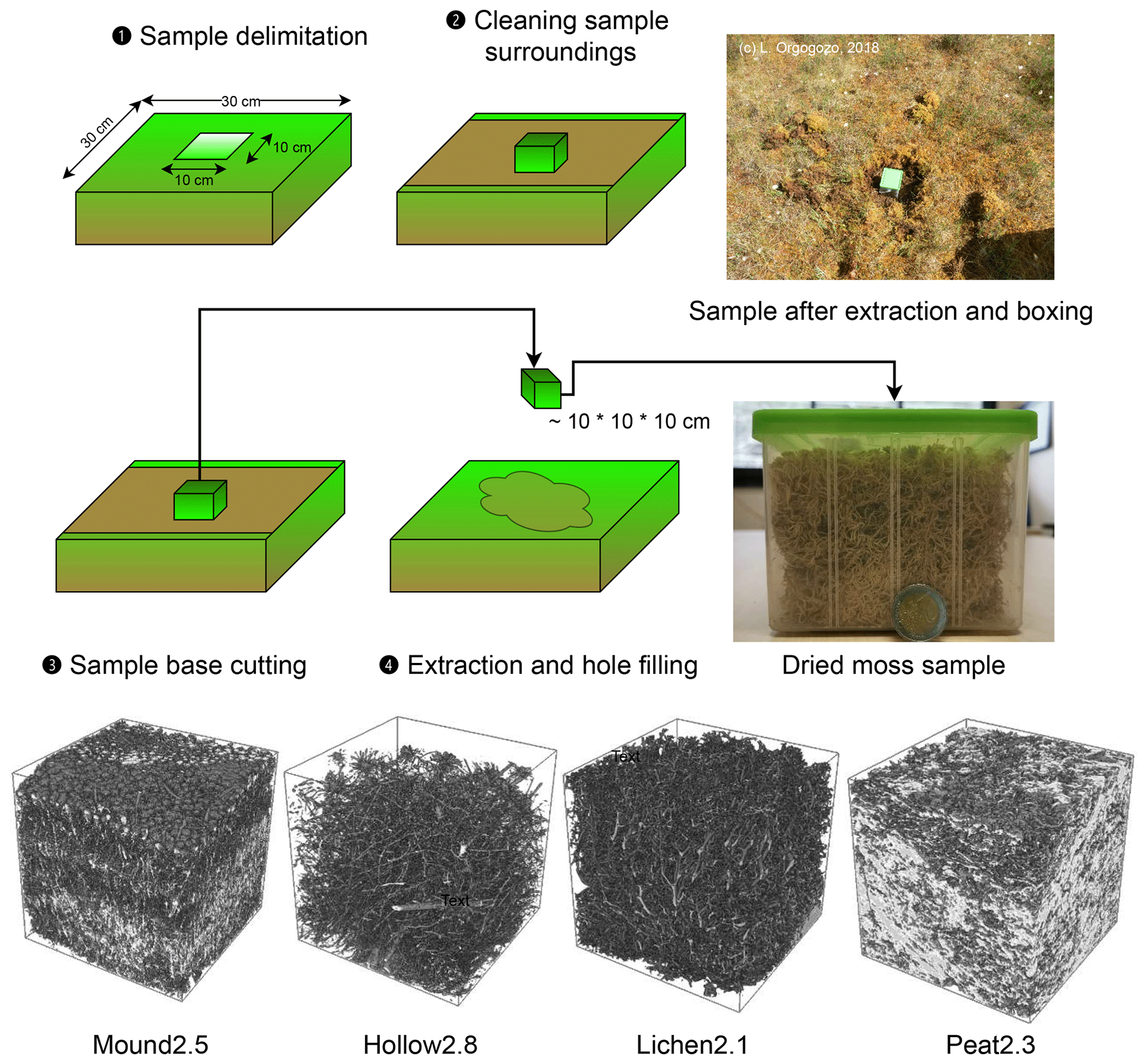
The samples are then dried at 40 ∘C for 48 h after sampling. Thereafter, each sample is scanned and digitally reconstructed using high-resolution X-ray imagery.
X-ray computed tomography (X-CT) has been widely studied and is extensively used for medical purposes and geoscientific applications (Christe et al., 2011). Tomography is a non-destructive technique which enables the observation of pore structure data at micron scale, especially for pore space assessment in sedimentary rocks. X-CT scanning has been acknowledged as being an efficient method for accessing morphological information, such as the pore structure of peat soils (Turberg et al., 2014). Cnudde and Boone (2013) published an exhaustive review of X-ray tomography applications for the Earth sciences. Rezanezhad et al. (2016) demonstrated that X-CT peat scanning showed a satisfactory spatial resolution for the study of peat's pore morphology. Since bryophytes can be assumed to represent a cluster of individuals, X-CT permits the segmenting of each plant structure, which cannot otherwise be achieved without destructive techniques. Tomographical scans of studied samples are produced using EasyTom®XL (RX Solutions, France) with a maximal X-ray emission source set to 90 kV. The obtained resolution, after tridimensional reconstruction, is 94 µm voxel−1, except for “Lichen2.1” at 88 µm voxel−1 (due to the scanning settings used specifically for this sample). The voxel number ranges from 4.8×10⁸ to 9.6×10⁸ voxels. Virtual samples are cropped and reduced to form a usable volume (UV) to avoid sampling border effects. Using ImageJ-Fiji (Schindelin et al., 2012), computed samples are then binarized using an intra-class variance-reducing algorithm (Otsu, 1979). This resulted in a sample consisting of an 8-bit black and white image stack. Supplement S1 contains some of the technical data, such as usable volumes and digital reconstructions, for each sample.
2.2 Drying impact assessment of sample representativity
The sampling locations and processing facilities were far away from each other. To ensure structural preservation, special care is taken throughout the sampling, transportation and scanning operations. The samples are oven-dried for 48 h at 40 ∘C, at atmospheric pressure, to halt biological degradation. As expected, Sphagnum mosses began to whiten and become papery, as described by Hayward and Clymo (1982). The samples are scanned at the Toulouse Institute of Fluid Mechanics under dry conditions, 2 months after their primary extraction at Khanymei Research Station and drying.
To ensure the dry samples' representativity, we used an analogous drying experimental protocol to the one carried out by Kämäräinen et al. (2018). This experiment is conducted on similar Sphagnum species (S. fuscum (Schimp.) H.Klinggr., S. majus (Russow) C.E.O. Jensen) and sampled according to the same method at Clarens mire (southwestern France, N43∘08′41.3", E0∘25′12.9") in March 2021, notwithstanding that Sphagnum acrotelm (growing section of a Sphagnum individual) is much thinner than Siberian samples. Four samples are collected, two being dried at 40 ∘C for 48 h and the other two being left untouched, as control samples. Each of the four samples is scanned 2 d after their extraction and then again 14 d after extraction. Additionally, one Sphagnum majus individual is extracted and left to dry under ambient conditions.
A comparative study between each of the two sample lots and the lone individual show that drying does not affect structural preservation. Our validation experiment converges with the results found by Kämäräinen et al. (2018). This also confirms hyaline cells' structural durability: the early work of Puustjärvi (1977) showed that hyaline cells were well preserved during biological decay. Drying impacts aside, Sphagnum's continuous growth on non-dried control samples seems the most impactful structural factor, as each individual was striving to adapt itself to the sampling box hydric conditions. Fast drying before tomographic examination can be a reasonable solution for preserving the morphological structure, in conjunction with careful on-site sampling.
2.3 Morphological analysis: total porosity (εtotal), open porosity (εopen), specific surface area (SSA) and pore size distribution
Global porosity (εTotal) is calculated for each sample using built-in ImageJ-Fiji tools and macro-scripting. Porosity is considered to be a ratio between the number of voxels representing the void phase ivoxel (void phase's internal volume, including closed porosity) over the total number of voxels representing a sample Ntotal (void and matrix volume). This relation is shown in Eq. (1):
Porosity is computed on bidimensional horizontal slices along the z axis to evaluate porosity variations along the samples. Image stacks are then reconstructed along the x and y axes to create two other image stacks. Finally, porosity is computed along the x, y and z axes using a voxel-counting algorithm shown in Sect. 3.1.
The samples could then be classified into three types according to the porosity profile along the vertical axis (Table 3 and Supplement S2). As porosity appears to be almost constant over the x and y axes, sample classification is solely based on vertical porosity z.
-
Type I: constant high porosity along the z axis, excluding border effects
-
Type II: low basal porosity, linearly increasing to the top of the sample
-
Type III: no specific trend observed in vertical porosity
For each sample nature as well as each classified type, a dedicated color palette is chosen and kept consistent throughout the study for the sake of clarity.
Table 3Computed global porosity (εtotal), ratio of open porosity (popen), classification (I, II, II) and average planar porosity (%) for each sample obtained using a voxel-counting algorithm.

Open and connected porosities (εopen) are retrieved using dedicated shape analysis and labeling tools provided in the IPSDK™image-processing toolkit (a Reactiv'IP product used in Goubet et al., 2021). This enables a precise segmentation to associate each connected void space into a unique identifier. Here, since the samples have more void than matter, this first label is assumed to be connected void space, which plays a major role in the flow and transfers (porosity), the latter being a closed or non-communicating element. From the raw dataset, voxel intensity is integrated to get the first label's voxel sum divided by the overall voxel number, as shown in Eq. (2):
The specific surface area is deduced using the same shape analysis and labeling tools included in IPSDK™. Integrating the surface between both phases (void and solid) yields the total surface S. Thus, volumetric-specific surface area SSA is obtained by dividing this surface by the sample's bounding box volume, expressed in m2 m−3, as shown in Eq. (3):
Specific surface area is conventionally expressed in relation to density (m2 g−1). For this purpose, each dried sample mass is obtained using an analytical balance and the sample's dry bulk density ρdry. Then, volumetric-specific surface values are converted into a mass-related specific surface by dividing volumetric-specific surface area by dry density, as shown in Eq. (4):
Pore size distribution is calculated using ImageJ-Fiji's implemented image segmentation tools on the binarized image stacks. In each stack's image, a Euclidean distance transformation of the matrix phase from the void phase is first applied. Then, for each isolated void patch, the Feret diameter is computed.
2.4 Darcy-scale morphological and hydrological property definition: REV
In this study, the collected samples are assumed to form a complex fibrous porous medium. Resolving mechanistic equations in such large domains is not straightforward due to the extensive computational resources required. Conversely, resolving such equations on an arbitrary cropped sample would not aid the hydraulic property assessment. To make the link between microscale and macroscale phenomena, a reproducible pattern is required to avoid microscale heterogeneities and lack of information due to a diminutive sample size. To do this, finding a representative region that validates scale separation assumptions with both microscale and macroscale heterogeneities is compulsory, thus defining the volumetric average of a microscale property that is continuous and informative at a macroscale. One of the first volume-averaging methods consists of finding a statistical REV for the given studied property.
Indeed, REV is a theoretical concept clarifying the definition of the macroscopic scale (Darcy scale) and the microscopic scale (pore scale) and characterizing a given porous medium. This REV can be assumed to be a specific sample volume in which transfer-governing equations (single-phase flow, for example) may be defined along with the associated effective properties. A proper mathematical definition of a REV is given in Bachmat and Bear (1987), Quintard and Whitaker (1989) and Whitaker (1999) along with a thorough definition of volume-averaging methods. A generic profile for a given property φβ is shown in Fig. 2.
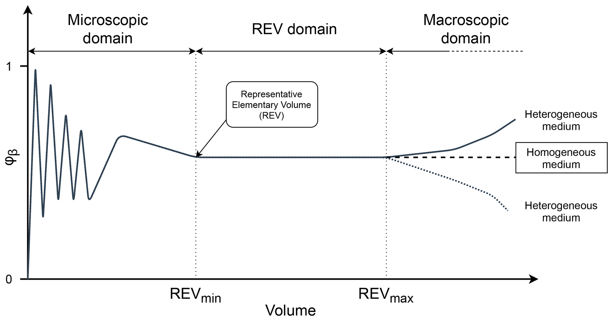
Figure 2Schematic representation of fluctuations of a generic property φβ in conjunction with volume (adapted following Brown and Hsieh, 2000).
The fluctuation profile shows three main domains. Here, the REV is defined as the smallest volume for which statistical fluctuations of a given property in a given space are sufficiently low to consider its average value an effective property. Finding the representative elementary volumes of some key properties (e.g., porosity and intrinsic permeability) is a routine workflow in porous-medium sciences. It is often used for fractured oil reservoirs (Durlofsky, 1991) or artificially packed glass bead media (Leroy et al., 2008). A REV is, by definition, large when compared to characteristic lengths of heterogeneities at a microscopic scale but small when compared to characteristic lengths of heterogeneities at the macroscopic scale. Thus, the properties computed for a REV of a porous medium may be defined and computed as continuous functions of space and even constant, in the case of a homogeneous porous medium, as defined by Bear (1972). In general, REVs are described on the basis of morphological characteristics such as porosity, although a distinct REV can be found for any given porous-medium property. Porosity and hydraulic-conductivity-related REVs are characterized throughout this study, leading to two different sizes, one for each property.
2.4.1 Porosity: binarization and voxel counting
From previously binarized image stacks, a statistical REV analysis is conducted using dedicated high-performance image processing Python libraries (IPSDK™), encapsulated in a specifically designed batch process for which the flowchart is shown in Fig. 3.
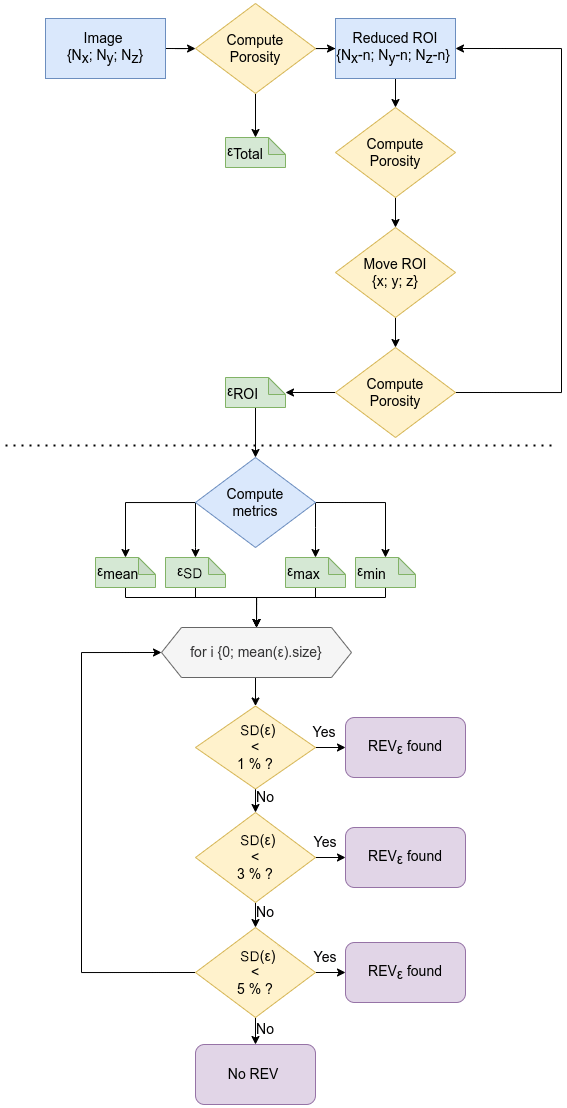
Figure 3Flowchart of the representative elementary volume of porosity (REVε) from a binarized image. For each sample, three thresholds are tested (5 %, 3 % and 1 % and standard deviation variation).
First, porosity (Eq. 1) is computed for a given sub-sampling volume within the whole sample. Then, the sub-sampling volume location is incrementally reduced and moved in every spatial direction. For each sub-volume, intermediate porosities are computed. The average and standard deviations are stored for each chosen sub-sampling volume. Then, an algorithmic routine is used to find the maximal size that satisfies a given threshold (1 %, 3 % or 5 % of porosity fluctuation). These thresholds define the statistical representativity of these REVs. Thus, a REV satisfying a 1 % threshold can be assumed to be a high-grade REV, whereas the 5 % threshold corresponds to lower-grade REVs. For 10 of the 12 studied samples, a REV of porosity is found. The two remaining samples, Hollow1.2 and Peat2.2, do not exhibit a REV for the chosen thresholds. A collection of tridimensional reconstructions of the samples as well as some examples of REVs for each sample are shown in Supplement S1. The graphical plots for each studied sample are available in Supplement S3. The black dot represents the smallest reached representative elementary volume for each sample.
2.4.2 Hydraulic conductivity: direct numerical simulation
Hydraulic conductivity is estimated through single-phase flow computations performed by solving a Navier–Stokes equation in the pore space of the considered sample. The concept is to carry out the numerical simulation of fluid flow, reproducing the conditions occurring in a constant-head (CHP) permeameter. Then, a sample's hydraulic conductivity is computed from the obtained velocity field. A virtual CHP is created by imposing a constant pressure on two opposite faces to one direction (inlet and outlet). Water-tight wall boundary conditions are applied to other faces, as shown in a conceptual representation of the initial and boundary conditions available in Supplement S2.
Due to computation time limitations, the biggest studied sub-volume with this approach corresponds to a quarter of the total sample. In Sect. 2.4, we stated that the REVs of effective physical properties were valid for that particular physical property. Thus, a hydraulic conductivity REV is required to statistically assess hydraulic conductivity. For that purpose, instead of counting voxel value algorithms (as made for porosity), retrieving a representative elementary volume for hydraulic conductivity requires extensive fluid mechanics simulations. Here, a laminar single-phase flow induced by a pressure gradient is computed for each sub-sample, being consistent with the idea of reducing and moving a defined sub-volume inside the overall sample. From open-porosity data in Table 3, we can show that most porosity is connected to each one. This leads to the assumption that considering all pores can be considered effective in permeability-driven phenomena. As these simulations are resource-costly, Type-I samples (constant porosity) are selected as they are sufficiently homogeneous for the establishment of REVs. Other types are treated by another method presented in Sect. 2.4.3. The implemented method relies on Mohammadmoradi and Kantzas (2016) in conjunction with automatic mesh manipulation tools (trimesh Python library, Dawson-Haggerty et al., 2019). For each Type-I sample, single-phase flow simulation through a fraction of the solid volume (representing a sample) is conducted. The simpleFoam algorithm is used to solve a velocity field from an initial pressure gradient. The simpleFoam solver is an enhanced version of the original SIMPLE algorithm (Semi-Implicit Method for Pressure-Linked Equations – Patankar, 1980) nested in the open-source Computational Fluid Dynamics toolkit OpenFOAM (Weller et al., 1998, https://openfoam.org/, last access: 17 January 2023; https://www.openfoam.com/, last access: 17 January 2023).
For each sample, four potential REV sizes are computed (23.5, 15.7, 11.8 and 9.4 mm), consisting of 8, 27, 64 and 125 simulations on the x, y and z axes, respectively, representing 672 simulations per sample. These sizes are chosen from the beginning to limit computation times, as using the same scanning method than what was developed for porosity is computationally prohibitive. This is run on the tier-2 supercomputer Olympe (CALMIP computational mesocenter, Toulouse, France). These calculations are run simultaneously, each occupying one node (36 physical cores), representing 10 500 h CPU (about 12 d of physical time) per sample. For each simulation, the velocity field ui is integrated with the overall outlet surface Soutlet (including the surface occupied by the solid matrix) to get an averaged outlet flux value vi, according to Eq. (5):
A careful convergence study is also conducted so that numerical errors, associated with discretization resolutions and iterative procedures for the approximated inversions of the linear systems involved, are low enough to be neglected in the analysis of the results. Inlet pressures are chosen to avoid turbulent flows (Re <<1). The computed Darcy velocity vi could then be injected into a regular Darcy law, as shown in Eq. (6), where kii is a tensorial component of intrinsic permeability (m2) and μw is the dynamic viscosity:
To avoid artifacts related to the physics of a specific fluid, the simpleFoam solver uses kinematic pressure (expressed in m2 s−2) and kinematic viscosity ν (m2 s−1) to solve Navier–Stokes equations. These equations are based on intrinsic permeability k expressed in m2. However, in the field of hydrology the hydraulic conductivity (m s−1), abbreviated to Kw, is generally used. One can relate hydraulic conductivity Kw to intrinsic permeability k by using Eq. (7) described by Claisse (2016).
In continental surface hydrology, liquid water's physical property variations (e.g., volumetric mass ρw and dynamic viscosity μw) are generally neglected. Thus, intrinsic permeability values obtained from the numerical computations were converted using water's thermodynamic properties at 293.15 K and 1.013 kPa (Chemical Rubber Company and Lide, 2004), considering the following conversion equation (Eq. 8):
This method is suitable for samples meeting porosity homogeneity requirements, classified into Type-I samples. However, another method is needed to compensate for Type-II and Type-III sample heterogeneity, as using direct numerical simulations on a complete usable volume is prohibitive in terms of computational resources. The results obtained for hydraulic conductivity REV computations are available in Supplement S4.
A double-ring infiltrometry test was also conducted during the sampling campaign. For the sake of comparison, hydraulic conductivity values obtained using this method are also shown in Table 2.
Table 4Obtained representative elementary volume based on porosity (REVε). is the side length of a cubic REV of porosity. is the average porosity of a given cubic REV. The ratio represents the volumetric percentage of the sample included in the REV.

2.4.3 No REV for hydraulic conductivity: use of PNM
For the samples that do not exhibit a REV for hydraulic conductivity (Type-II and Type-III samples), the hydraulic conductivity is then studied using a pore network model, generated from the binarized image stacks. Pore network models are based on the structural simplification of a complex pore structure (rocks or reactive porous industrial media, for example) into a two-state model: spheres and throats. This method often uses various image processing and segmentation tools to generate a network of spheres and linking throats, based on an initial tridimensional volume. Introduced by Fatt (1956), pore network modeling was first studied in conjunction with predefined network properties. Then, pore network generation was adapted to model some porous media, scanned with X-ray tomography using image-processing algorithms as accurately as possible (Dong and Blunt, 2009). Various algorithms are used to create the internal pore network structure, such as the maximal ball algorithm (Silin and Patzek, 2006). More recently, other algorithms based on the morphological properties of the studied porous media have emerged, such as the Sub-Network of the Oversegmented Watershed (SNOW) algorithm (Gostick, 2017). This alternative algorithm is considered to be computationally efficient, allowing a porous medium to be accurately modeled by numerical imagery (Khan et al., 2020). The SNOW algorithm showed a good fit with the standard maximal ball algorithm. Generating a pore network and simulating a flow in it is often cheaper, in terms of computational resources, when compared to direct numerical simulation. However, more complex transfer mechanisms, such as imbibition and drainage, are still in the study phase, and some extensive work on computational optimization has yet to be conducted, specifically on non-user-generated porous media (Maalal et al., 2021).
For each binarized Type-II and Type-III image stack, a direct pore network extraction is conducted using the SNOW algorithm implemented in the OpenPNM and PoreSpy open-source Python libraries (Gostick et al., 2019). Then, a synthetic porosity and a synthetic specific surface area may be computed for the obtained simplified representation of the pore space of the porous medium. Using the implemented Stokes equation solver, a diagonal permeability tensor is retrieved from the generated pore networks, applying the identical boundary conditions based on the method given by Sadeghi and Gostick (2020). Once again, intrinsic permeability tensors are converted into a hydraulic conductivity tensor using the relation in Eq. (8).
In Supplement S5, a comparative study is described based on Type-I samples between both developed workflows. Then, some clues are given as to whether DNS or PNM is suitable for a given sample.
3.1 Morphological analysis
The global-porosity and open-porosity proportion (popen) for each sample is shown in Table 3, ranging from less than 40 % (Mound1.1) to more than 95 % (Hollow2.7).
On average, lichens are the most porous of the collection, and peat is the least porous. Porosity values are in line with previously obtained data from the literature for the highest porous media of the collection (Yi et al., 2009). However, important variability can be observed for Sphagnum samples, gathering minimal and maximal porosity values. Mound mosses have an average porosity of 65.9±22.3 %, whereas the average hollow moss sample porosity is 79.6±20.2 %. Porosity profiles for each sample are presented in Fig. 4.
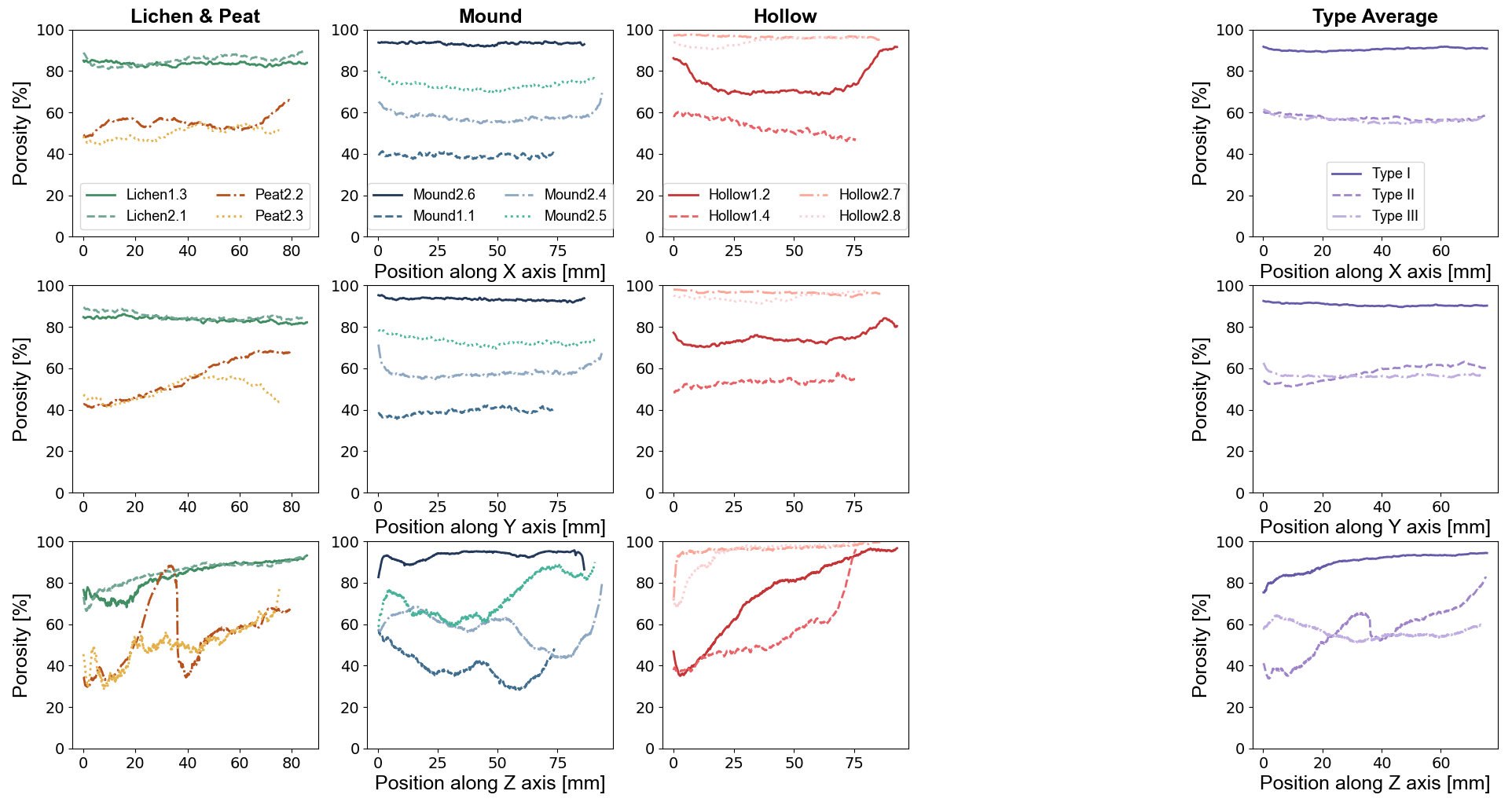
Figure 4Planar porosity plot along the x, y and z axes for moss, lichen and peat samples. An averaged value is computed for each sample type, each color nuance representing each type. Type I: stable high-porosity profile samples, excluding border effects. Type II: low basal porosity, linearly increasing to the top of the sample. Type III: no specific trend observed in vertical porosity.
No specific trend can be accessed from the x- and y-axis porosity profiles, and yet variations can be observed on the z axis. Again, three trends can be observed, clustering samples into three groups according to their respective porosity profile trends.
-
Type I: stable high-porosity profile samples, excluding border effects (εtotal>80 %): Mound2.6, Hollow2.7, Hollow2.8, Lichen2.1, Lichen1.3
-
Type II: medium- to high-porosity profile samples associated with a progressive increase from the bottom to the top: Hollow1.2, Hollow1.4, Peat2.2, Peat2.3
-
Type III: medium to low porosity associated with no specific trend porosity profiles: Mound1.1, Mound2.4, Mound2.5.
The Type-I class contains both lichen samples (Lichen2.1, Lichen1.3), whereas Type III only consists of mound Sphagnum (Mound1.1, Mound2.4, Mound2.5). The Type-II class contains half of the hollow Sphagnum samples as well as both peat samples (Peat2.2, Peat2.3).
Open and connected porosity (popen, Table 3) represents nearly all the void space volume in each sample. Open porosity ratio values range from 0.99 to 0.9999. Thus, we can assume that, due to the fibrous nature of the studied material, enclosed porosity does not play a major role in the flow dynamics of the studied samples.
Pore size distribution (Fig. 5) is heterogeneous in each sample, and the sizes are concentrated between 0.01 and 1.00 mm of pore radii. The median pore size varies from 0.23 mm (for peat samples) up to 0.88 mm (for lichen samples).
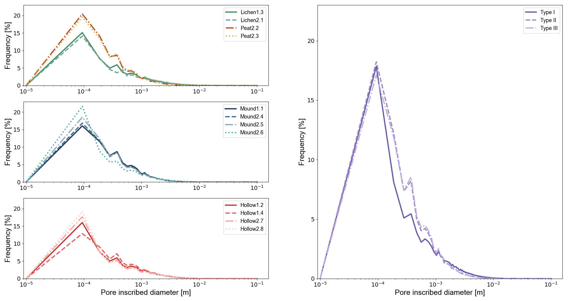
Figure 5Inscribed pore size distribution by classified type using particles' Feret diameter measurement. An averaged value is computed for each sample type, each color nuance representing each type.
Intermediate median pore size values can be found for mound Sphagnum samples at average values between 0.34 and 0.70 mm (for hollow Sphagnum samples). According to the previous classification, the median pore size for each sample type (I, II and III) is 0.66, 0.42 and 0.33 mm, respectively. While Type-II and Type-III curves differ in bidimensional porosity along z, they share similar global pore size distributions. Type-I samples are distinct from Type-II and Type-III curves. Specific surface area (SSA) values for each sample are shown in Fig. 6.
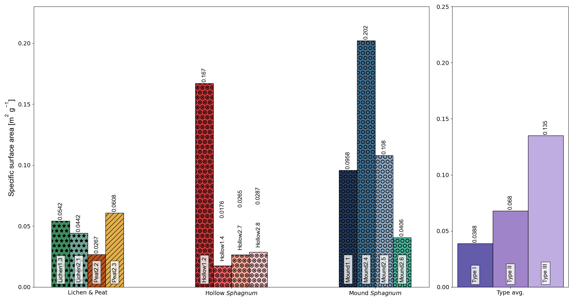
Figure 6Specific surface area (m2 g−1) plots for each sample. Colors refer to each sample type.
Specific surface area values seem to be uneven between each sample type. For instance, low specific surface areas can be observed for some hollow Sphagnum samples ( and m2 g−1 for Hollow2.7 and Hollow2.8, respectively). Higher specific area values can be found for one mound of Sphagnum ( m2 g−1 for Mound2.4) and for one hollow Sphagnum sample ( m2 g−1 for Hollow1.2).
3.2 Porosity
Representative elementary volumes for porosity have been computed when possible. For samples exhibiting a REV, porosity has been computed using Eq. (1) applied to the REV. For samples admitting no REV, porosity has still been computed using Eq. (1) but applied to the whole usable volume of the sample. A REV retrieval algorithm was applied to all 12 studied samples, although 2 of them (Hollow1.2 and Peat2.2) did not admit a REV. Obtained REV sizes are shown in Table 4. Some examples of tridimensional visualizations of REVs of porosity are shown in Supplement S1. Due to the numerous graphs obtained during REV computation, tridimensional porosity plots are available in Supplement S3.
REVε sizes vary from 2 mm to 2 cm, representing 8.0×10³ to 2.19×10⁶ voxels. Substantial morphological variations are visible, spanning from simple tubular structures (visible in the REV of Hollow2.7) to a complex and fibrous medium (for the Mound2.6 sample, Supplement S1). The average porosity obtained for these REVs (shown in Supplement S3) varies from 83.4 % to 96.0 %, which confirms the high porosity factor of these biological media. Computation times for porosity–REV retrieval range from 3 to 6 h, using two Intel® Xeon® E5-2680 v2 (2.80 GHz) processors and 128 GB of RAM, using high-performance Python image-processing libraries (IPSDK™). Graphical synthesis of the digital porosity assessment is presented in Fig. 7.
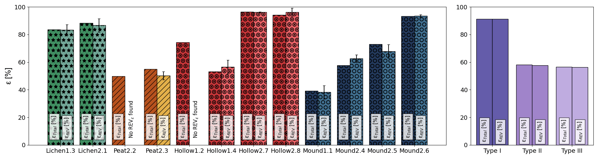
Figure 7Numerical porosity estimations (%) for each sample. An averaged value is computed for each identified sample type (I, II, III) with corresponding color nuances. Peat 2.2 and Hollow1.2 did not admit any REV.
3.3 Hydraulic conductivity
Due to the time and computational resources needed to achieve a careful study of a representative elementary volume of hydraulic conductivity, only Type-I samples were studied by DNS, as they represent the most homogeneous samples of the collection. Computed REVs of the hydraulic conductivity sizes are given in Table 5. Diagonal hydraulic conductivity tensor components are shown in Fig. 8, and box plots are available in Supplement S4. Computations for the largest sub-sample size (on a 23.5 mm edge) showed higher component hydraulic conductivity values than for the three smaller sizes. This discrepancy can be related to an insufficient computation number for obtaining a good average value, hence the wider statistical spread around the mean value. Moreover, the higher values for the largest studied sizes can also be correlated with heterogeneous hydraulic conductivity behavior, as theoretically shown in Fig. 2, such as effects related to the existence of macropores. An example of a pressure field obtained on a sub-sample of Hollow2.8 through DNS is shown in Fig. 9b.
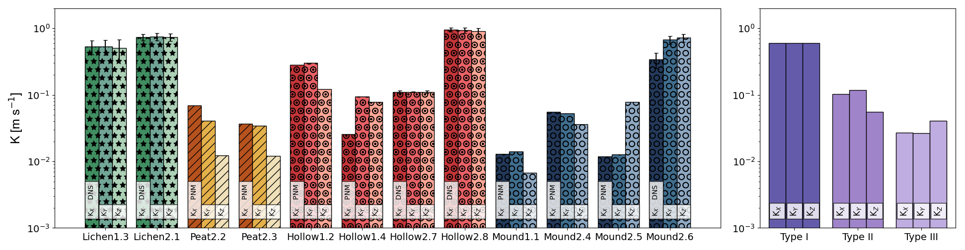
Figure 8Diagonal components of the hydraulic conductivity tensor (m s−1) on the x (Kxx), y (Kyy) and z axes (Kzz) based on DNS on a representative elementary volume of hydraulic conductivity (REVK) for Type-I samples and with a PNM for Type-II and Type-III samples.
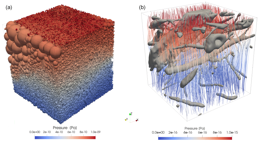
Figure 9(a) Pressure field (Pa) after a single-phase flow simulation thorough a pore network model based on a Mound2.5 sample. Spherical pore sizes are represented according to their respective size in the network. (b) Pressure field lines (Pa) after a single-phase flow simulation through a sub-sample of the Hollow2.8 sample. The gray mesh corresponds to the isolated biological phase.
Table 5Diagonal components of the hydraulic conductivity tensor (m s−1) for the studied REVK for Type-I samples using direct numerical simulations.
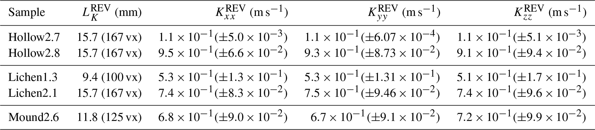
For three of the Type-I samples, REVK length is computed as 15.7 mm, which is the second-largest computed size. Variations in hydraulic conductivity, with respect to study volume reduction, are smaller than those found for porosity, although study points were scarcer in the case of hydraulic conductivity assessment. Lichen1.3 shows the smallest REVK. It can be seen that the smallest REVε was also described for Lichen1.3. Size differences can be seen between REVε and REVK, up to 5 times larger for Lichen1.3 and half the REVε for Mound2.6. This seems to show that the representative elementary volume found for porosity cannot accurately describe properties such as hydraulic conductivity. This is often the case, as porosity REV is smaller than the REVs defined for other properties (Zhang et al., 2000; Costanza-Robinson et al., 2011).
Numerical estimations of hydraulic conductivity are presented in Fig. 8. For each sample of Type I, the axial components of the hydraulic conductivity tensor are given, based on the representative elementary volume of hydraulic conductivity. For Type-II and Type-III samples, hydraulic conductivity estimates are given based on pore network modeling. An example of pressure field computation is shown on sample Mound2.5 in Fig. 9a. Using a pore network allows the estimation of properties in a model based on the whole sample. The use of a pore network is an affordable alternative to direct numerical simulations at the cost of accuracy.
The values obtained vary from to m s−1 for Type-I samples and from to m s−1 for Type-II and Type-III samples. Type-I samples can be assumed to be highly water-conductive biological media. Mean hydraulic conductivity decreases when the computed region size becomes smaller, for each direction and each sample (Supplement S4). In situ measurements, conducted by infiltration (Table 2), give an average of 10−5 m s−1, which is on the same order of magnitude as previously published field measurements (Crockett et al., 2016) and computed values (McCarter and Price, 2012). Analogous values for vertical hydraulic conductivity have been found in the literature at m s−1 (Päivänen, 1973; Crockett et al., 2016; Golubev et al., 2021). However, other studies showed results of a different order of magnitude for Sphagnum samples, with values under 10−4 m s−1 (Hamamoto et al., 2016). These differences could be explained by the experimental method used to retrieve hydraulic conductivity as well as Sphagnum bog oscillation occurring during sampling (mire breathing) (Strack et al., 2009; Golubev and Whittington, 2018; Howie and Hebda, 2018), which is going to be discussed in the next part.
Digital assessments of the morphological and hydraulic properties of Sphagnum and lichens of the Western Siberian Lowlands presented in this work suggest extremely porous, connected media with high specific surfaces and high hydraulic conductivities. These results are in line with the biogeochemical observations of Shirokova et al. (2021), demonstrating the overwhelming role of Sphagnum mosses in organic carbon, nutrient and inorganic solute fluxes in the Western Siberian Lowlands. Nonetheless, discrepancies between the numerical results presented in this work (Figs. 7 and 8) and previously published measurements of the hydraulic properties of Sphagnum are noteworthy (Table 2). Weaker but still sizeable differences can be seen between the results given by both of the numerical methods used here for the estimation of hydraulic conductivity on the same sample, namely, DNS and PNM. This last methodological point is discussed in Supplement S5, where a comparative validation is performed between DNS and PNM on homogeneous samples (Type I).
4.1 Numerical reconstruction after scanning
Due to technical limitations, scanning devices have a minimal resolution that causes a loss of information, acting as a threshold. In this study, minimal resolution fluctuated between 88 and 94 mum voxel−1, meaning that two elements of this size could not be distinguished. In our study, technically unreachable porosity (porosity that is smaller than the minimal scanning resolution) is assumed to play a negligible role in transfers through a saturated medium, reacting as an enclosed porosity. Pre-processing algorithms (especially binarization) can cause information loss due to the arbitrary categorization of each voxel. This erroneous description can be seen for small elements (such as Sphagnum leaves) which shrink them. Mesh generation may also bring some additional “over-erosion” that helps flows inside a sample. These impacts could be studied by reducing scanning resolution, albeit not available at the time of the scans. However, hydraulic conductivity overestimation in DNS that could be related to these pre-processing effects is likely to be negligible. Indeed, the high porosities encountered and the preferential flow paths that occur in the largest pores (macropores) predominate over enclosed pore dynamics. This might not be the case for unsaturated hydraulic property assessments.
4.2 Numerical results vs. field experiments: porosity and specific surface
As described in previous sections of this study, the samples collected are considerably porous. Porosity values are in line with past results found in the literature (Yi et al., 2009; Kämäräinen et al., 2018), with porosities above 90 % for some of the samples. Interestingly, a volumetric digital-specific surface can be well linked with the porosity of complete samples as well as the average porosities found for representative elementary volumes.
A clustering can be seen for the three studied sample types (Fig. 10), although mathematical relations between specific surface and porosity are not well defined for such porous media. The specific surface values obtained are of the same magnitude as previous values obtained for other natural moss and lichen species using geometrical calculations ( m2 g−1 for Hypnum cupressiforme (Hedw., 1801) moss and m2 g−1 for Pseudevernia furfuracea ((L.) Zopf, 1903) lichen in Adamo et al., 2007). These values are still notably lower than the values obtained using the B.E.T. method of N2 adsorption isotherms (1.1×101m2 g−1 for artificially grown Sphagnum denticulatum (Brid., 1926) in Gonzalez et al., 2016). As discussed in Sect. 4.1, a lack of micropores could explain the observed discrepancies (1 to 2 orders of magnitude) between calculated geometry and B.E.T.
Figure 10Specific surface (m−1) as a function of total porosity εTotal (%) and representative elementary averaged porosity (%).
4.3 Numerical results vs. field experiments: hydraulic conductivity
In Supplement S5, a comparison between direct numerical simulations and pore network modeling is made showing that pore network modeling is suitable for bypassing the heterogeneity issues observed in our samples. Indeed, the obtained porosity values with PNM are in a 5 % threshold compared to voxel-counting results (Eq. 1). The hydraulic conductivities computed by PNM and DNS are more contrasted, with 1 to 2 orders of magnitude of difference. One should bear in mind that the range of hydraulic conductivity of natural porous media is huge, with up to 15 orders of magnitude between coarse gravel (10−1 m s−1) and unweathered shale (10−15 m s−1). Besides this, it is logical that the simplifications involved in the PNM method result in information loss compared to the DNS method. On the other hand, computational time savings (by using the PNM method) are huge (counted in tens of days for DNS and hours for PNM). In some cases (e.g., samples of Types II and III), DNS is simply not possible with the current regional-scale supercomputing means.
The obtained numerical hydraulic conductivities tend to show high and relatively isotropic hydraulic conductivity tensor values. Hydraulic conductivities found using DNS are sizably higher than previous values found in the literature using field percolation (Table 2), often by up to 1 to 3 orders of magnitude. The hydraulic conductivities found using pore network modeling seem to be more in line with the values in Table 2 as well as the field experiment results shown in Table 6. Nevertheless, it should be kept in mind that the results obtained by this method are less structurally accurate that those obtained from DNS, since they rely on a simplified description of the pore structure. Some clues can be advanced to explain this discrepancy, the first being the impact of numerical reconstruction routines and mesh generation procedures (discussed in Sect. 4.1), the latter being moss compression during field experiments.
Table 6Hydraulic conductivity values (m s−1) obtained using a double-ring infiltrometer during the sampling campaign.
Our digital, constant-head permeameter experiments were conducted in a fully saturated medium. Technically unreachable porosity (porosity that is smaller than the minimal scanning resolution) is assumed to play a negligible role in transfers through a saturated medium, reacting as enclosed porosity. In the case of low-permeability porous media, such sub-resolution porosity may affect flow (Soulaine et al., 2016). However, in the case of highly porous and connected media like mosses and lichens, the effects related to sub-resolution porosity are assumed to be low when compared to the effects of the large macropores, which has been shown by Baird (1997). It should also be noted that most of the porosity is opened and connected in our case.
However, moss and lichen samples are compressible (Golubev and Whittington, 2018; Howie and Hebda, 2018; Price and Whittington, 2010). Field percolation experiments induce a sizeable and rapid mass imbalance on this bryophytic cover, compacting the pore space more than would occur under natural rainfall conditions. This might notably affect flow patterns in macropores and explain the lower hydraulic conductivities found in field experiments. Indeed, some clues are given with the results of Weber et al. (2017) on hydraulic conductivity variations according to water saturation. Therefore, the numerical hydraulic conductivity assessments carried out in this study enable property quantification of the medium without perturbation, such as compression of the biological pore structure, which is not possible in field experiments.
A numerical assessment of morphological and hydraulic properties was carried out on digital X-CT reconstructions of samples of Sphagnum moss, lichen and peat from the Western Siberian Lowlands' bryophytic cover. This porous-medium-centered approach confirmed the high porosities (from 70 % to 95 % for most samples) already found in previous studies involving experimental measurements. Hydraulic conductivity estimation was conducted using direct numerical simulations for Type-I samples and pore network modeling for Type-II and Type-III samples, both fluctuating around 10−1 m s−1. Indeed, both methods used in this study converge to classify macroscopic lichen, Sphagnum moss and peat as being considerably porous and pervious biological media. The hydraulic conductivity tensor shows isotropic horizontal components; however, some differences can be seen, particularly in the vertical component. Both methods reach higher values than seen before in the literature. This may have been caused by interfering phenomena, such as moss compressibility, occurring during field experiments.
The methods developed for this application show that a numerical work scheme based on image processing allows retrieval of the morphological properties of any variety of sample. Using such a method permits a nearly unlimited number of property assessments of the same sample, whereas an experimental work scheme requires many samples. Numerical methods enable a qualitative classification of the overall homogeneity of a sample, which is not easily doable using solely experimental methods. Image processing seems to be a satisfactory method, provided that the studied sample is sufficiently homogeneous for the studied property. For heterogeneous samples, image processing is not optimal. However, in the absence of another method, pore network modeling allows us to obtain some information on the studied property which is close to the one found for the homogeneous samples using image processing.
These results provide firm ground for quantitative hydrological modeling of the bryophytic cover in permafrost-dominated peatland catchments, which is crucially important for a better understanding of the global climate change impacts on arctic areas. Using numerical methods potentially enables the assessment of moss and lichen's structural hydraulic conductivity without disturbance by any biological or physical phenomena. Therefore, the porous-medium approaches developed throughout this study led to unprecedented qualitative and quantitative descriptions of such peculiar, highly porous biological media.
These physical properties can then be used as input parameters to describe ground vegetation layers in high-resolution hydrological models of arctic hydrosystems and extensively refine simulations of this critical compartment of boreal continental surfaces. For example, they will be used in further modeling studies of permafrost under climate change at the Khanymei Research Station in the framework of the HiPerBorea project (hiperborea.omp.eu). Further studies are needed to assess variable water content consequences for peat and vegetation pore structure. Indeed, water content is one of the main drivers controlling effective transport properties, such as unsaturated flow, volume change and thermal conductivity.
Material is available on the project's website (https://hiperborea.omp.eu/, Orgogozo, 2020).
The supplement related to this article is available online at: https://doi.org/10.5194/hess-27-431-2023-supplement.
Founding acquisition and project administration was handled by Laurent Orgogozo. The conceptualization, supervision and validation of this paper were conducted by Manuel Marcoux and Laurent Orgogozo. The original investigation, analysis, data curation, software engineering and writing of the original draft were done by Simon Cazaurang. Resources and field methodology were brought by Sergey Loiko, Artem Lim, Stéphane Audry, Liudmila Shirokova, Oleg Pokrovsky and Georgiy Istigechev. The original internal review upon submission was conducted by Manuel Marcoux, Laurent Orgogozo, Sergey Loiko, Artem Lim, Stéphane Audry, Liudmila Shirokova and Oleg Pokrovsky.
The contact author has declared that none of the authors has any competing interests.
Publisher's note: Copernicus Publications remains neutral with regard to jurisdictional claims in published maps and institutional affiliations.
This work was granted access to the HPC resources of the CALMIP supercomputing center under the allocation 2020-(p12166). Partial support from the Tomsk State University Development Program (“Priority-2030”) is also acknowledged. Sergey Loiko and Artem Lim thank the Russian Science Foundation (project no. 18-77-10045) for supporting the field work and Georgiy Istigechev for his help with the double-ring infiltrometry. The authors thank Laurent Bernard and Romain Abbal of Reactiv'IP for their support regardin the developments of the digital characterizations with IPSDK (tm) The authors also want to thank the Clarens Mire steering committee (http://tourbiere-clarens.n2000.fr/, last access: 20 March 2021) for giving us the permission to collect samples.
This research has been supported by the Agence Nationale de la Recherche (grant no. ANR-19-CE46-0003-01), the Centre National de la Recherche Scientifique (grant BryophyGel “Défi InFinitTI 2018 – 237579”), the Ambassade de France à Moscou (PHC Kolmogorov project 2017 N 38144TB), and the Russian Science Foundation (project no. 18-77-10045).
This paper was edited by Philippe Ackerer and reviewed by Xiaoying Zhang and one anonymous referee.
Aalto, J., Karjalainen, O., Hjort, J., and Luoto, M.: Statistical Forecasting of Current and Future Circum-Arctic Ground Temperatures and Active Layer Thickness, Geophys. Res. Lett., 45, 4889–4898, https://doi.org/10.1029/2018GL078007, 2018.
Adamo, P., Crisafulli, P., Giordano, S., Minganti, V., Modenesi, P., Monaci, F., Pittao, E., Tretiach, M., and Bargagli, R.: Lichen and moss bags as monitoring devices in urban areas. Part II: Trace element content in living and dead biomonitors and comparison with synthetic materials, Environ. Pollut., 146, 392–399, https://doi.org/10.1016/j.envpol.2006.03.047, 2007.
Bachmat, Y. and Bear, J.: On the Concept and Size of a Representative Elementary Volume (Rev), in: Advances in Transport Phenomena in Porous Media, edited by: Bear, J. and Corapcioglu, M. Y., Springer Netherlands, Dordrecht, 3–20, https://doi.org/10.1007/978-94-009-3625-6_1, 1987.
Baird, A.: Field estimation of macropore functioning and surface hydraulic conductivity in a fen peat, Hydrol. Process., 3, 287–295, https://doi.org/10.1002/(SICI)1099-1085(19970315)11:3<287::AID-HYP443>3.0.CO;2-L, 1997.
Banfield, J. F., Barker, W. W., Welch, S. A., and Taunton, A.: Biological impact on mineral dissolution: Application of the lichen model to understanding mineral weathering in the rhizosphere, P. Natl. Acad. Sci. USA, 96, 3404–3411, https://doi.org/10.1073/pnas.96.7.3404, 1999.
Bear, J.: Dynamics of fluids in porous media, Dover Publications, New York, 764 pp., ISBN 978-0-486-65675-5, 1972.
Bense, V. F., Kooi, H., Ferguson, G., and Read, T.: Permafrost degradation as a control on hydrogeological regime shifts in a warming climate: Groundwater and degrading permafrost, J. Geophys. Res., 117, F030036, https://doi.org/10.1029/2011JF002143, 2012.
Bernard-Jannin, L., Binet, S., Gogo, S., Leroy, F., Défarge, C., Jozja, N., Zocatelli, R., Perdereau, L., and Laggoun-Défarge, F.: Hydrological control of dissolved organic carbon dynamics in a rehabilitated Sphagnum-dominated peatland: a water-table based modelling approach, Hydrol. Earth Syst. Sci., 22, 4907–4920, https://doi.org/10.5194/hess-22-4907-2018, 2018.
Bernier, P. Y., Desjardins, R. L., Karimi-Zindashty, Y., Worth, D., Beaudoin, A., Luo, Y., and Wang, S.: Boreal lichen woodlands: A possible negative feedback to climate change in eastern North America, Agr. Forest Meteorol., 151, 521–528, https://doi.org/10.1016/j.agrformet.2010.12.013, 2011.
Biskaborn, B. K., Smith, S. L., Noetzli, J., Matthes, H., Vieira, G., Streletskiy, D. A., Schoeneich, P., Romanovsky, V. E., Lewkowicz, A. G., Abramov, A., Allard, M., Boike, J., Cable, W. L., Christiansen, H. H., Delaloye, R., Diekmann, B., Drozdov, D., Etzelmüller, B., Grosse, G., Guglielmin, M., Ingeman-Nielsen, T., Isaksen, K., Ishikawa, M., Johansson, M., Johannsson, H., Joo, A., Kaverin, D., Kholodov, A., Konstantinov, P., Kröger, T., Lambiel, C., Lanckman, J.-P., Luo, D., Malkova, G., Meiklejohn, I., Moskalenko, N., Oliva, M., Phillips, M., Ramos, M., Sannel, A. B. K., Sergeev, D., Seybold, C., Skryabin, P., Vasiliev, A., Wu, Q., Yoshikawa, K., Zheleznyak, M., and Lantuit, H.: Permafrost is warming at a global scale, Nat. Commun., 10, 264, https://doi.org/10.1038/s41467-018-08240-4, 2019.
Boelter, D. H.: Important Physical Properties of Peat Materials, 3rd International Peat Congress, Quebec, Cananada, 150–154, https://www.nrs.fs.usda.gov/pubs/jrnl/1968/nc_1968_boelter_001.pdf (last access: 21 February 2021), 1968.
Brown, G. O. and Hsieh, H. T.: Evaluation of laboratory dolomite core sample size using representative elementary volume concepts, Water Resour. Res., 36, 1199–1207, https://doi.org/10.1029/2000WR900017, 2000.
Brown, J., Ferrians, O. J., Heginbottom Jr., J. A., and Melnikov, E. S.: Circum-arctic map of permafrost and ground-ice conditions, USGS, ISBN 0-607-88745-1, 1997.
Burke, E. J., Zhang, Y., and Krinner, G.: Evaluating permafrost physics in the Coupled Model Intercomparison Project 6 (CMIP6) models and their sensitivity to climate change, The Cryosphere, 14, 3155–3174, https://doi.org/10.5194/tc-14-3155-2020, 2020.
Chemical Rubber Company and Lide, D. R. (Eds.): CRC handbook of chemistry and physics: a ready-reference book of chemical and physical data, 85. edn., CRC Press, Boca Raton, ISBN 978-0-8493-0485-9, 2004.
Christe, P., Turberg, P., Labiouse, V., Meuli, R., and Parriaux, A.: An X-ray computed tomography-based index to characterize the quality of cataclastic carbonate rock samples, Eng. Geol., 117, 180–188, https://doi.org/10.1016/j.enggeo.2010.10.016, 2011.
Claisse, P. A.: Transport of fluids in solids, in: Civil Engineering Materials, Elsevier, 83–90, https://doi.org/10.1016/B978-0-08-100275-9.00009-7, 2016.
Clayton, L. K., Schaefer, K., Battaglia, M. J., Bourgeau-Chavez, L., Chen, J., Chen, R. H., Chen, A., Bakian-Dogaheh, K., Grelik, S., Jafarov, E., Liu, L., Michaelides, R. J., Moghaddam, M., Parsekian, A. D., Rocha, A. V., Schaefer, S. R., Sullivan, T., Tabatabaeenejad, A., Wang, K., Wilson, C. J., Zebker, H. A., Zhang, T., and Zhao, Y.: Active layer thickness as a function of soil water content, Environ. Res. Lett., 16, 055028, https://doi.org/10.1088/1748-9326/abfa4c, 2021.
Cnudde, V. and Boone, M. N.: High-resolution X-ray computed tomography in geosciences: A review of the current technology and applications, Earth-Sci. Rev., 123, 1–17, https://doi.org/10.1016/j.earscirev.2013.04.003, 2013.
Costanza-Robinson, M. S., Estabrook, B. D., and Fouhey, D. F.: Representative elementary volume estimation for porosity, moisture saturation, and air-water interfacial areas in unsaturated porous media: Data quality implications, Water Resour. Res., 47, https://doi.org/10.1029/2010WR009655, 2011.
Crockett, A. C., Ronayne, M. J., and Cooper, D. J.: Relationships between vegetation type, peat hydraulic conductivity, and water table dynamics in mountain fens: Relating Vegetation Type and Peat Hydraulic Conductivity in Mountain Fens, Ecohydrol., 9, 1028–1038, https://doi.org/10.1002/eco.1706, 2016.
Dawson-Haggerty et al.: trimesh [online], https://trimsh.org/ (last access 19 May 2021), 2019.
Dong, H. and Blunt, M. J.: Pore-network extraction from micro-computerized-tomography images, Phys. Rev. E, 80, 036307, https://doi.org/10.1103/PhysRevE.80.036307, 2009.
Du, X., Loiselle, D., Alessi, D. S., and Faramarzi, M.: Hydro-climate and biogeochemical processes control watershed organic carbon inflows: Development of an in-stream organic carbon module coupled with a process-based hydrologic model, Sci. Total Environ., 718, 137281, https://doi.org/10.1016/j.scitotenv.2020.137281, 2020.
Durlofsky, L. J.: Numerical calculation of equivalent grid block permeability tensors for heterogeneous porous media, Water Resour. Res., 27, 699–708, https://doi.org/10.1029/91WR00107, 1991.
Elliott, J. and Price, J.: Comparison of soil hydraulic properties estimated from steady-state experiments and transient field observations through simulating soil moisture in regenerated Sphagnum moss, J. Hydrol., 582, 124489, https://doi.org/10.1016/j.jhydrol.2019.124489, 2020.
Fabre, C., Sauvage, S., Tananaev, N., Srinivasan, R., Teisserenc, R., and Sánchez Pérez, J.: Using Modeling Tools to Better Understand Permafrost Hydrology, Water, 9, 418, https://doi.org/10.3390/w9060418, 2017.
Fatt, I.: The Network Model of Porous Media, 207, 144–181, https://doi.org/10.2118/574-G, 1956.
Fox-Kemper, B., Hewitt, H. T., Xiao, C., Aðalgeirsdóttir, G., Drijfhout, S. S., Edwards, T. L., Golledge, N. R., Hemer, M., Kopp, R. E., Krinner, G., Mix, A., Notz, D., Nowicki, S., Nurhati, I. S., Ruiz, L., Sallée, J. B., Slangen, A. B. A., and Yu, Y.: Ocean, Cryosphere and Sea Level Change, in: Climate Change 2021: The Physical Science Basis. Contribution of Working Group I to the Sixth Assessment Report of the Intergovernmental Panel on Climate Change, edited by: Masson-Delmotte, V., Zhai, V. P., Pirani, A., Connors, S. L., Péan, C., Berger, S., Caud, N., Chen, Y., Goldfarb, L., Gomis, M. I., Huang, M., Leitzell, K., Lonnoy, E., Matthews, J. B. R., Maycock, T. K., Waterfield, T., Yelekçi, O., Yu, R., and Zhou, B., Cambridge University Press, https://www.ipcc.ch/report/ar6/wg1/chapter/chapter-9/, last access: 16 January 2023.
Galvin, L.: Physical properties of Irish peats, 207–221, https://www.jstor.org/stable/25555820 (last access 7 June 2022), 1976.
Genxu, W., Tianxu, M., Juan, C., Chunlin, S., and Kewei, H.: Processes of runoff generation operating during the spring and autumn seasons in a permafrost catchment on semi-arid plateaus, J. Hydrol., 550, 307–317, https://doi.org/10.1016/j.jhydrol.2017.05.020, 2017.
Golubev, V. and Whittington, P.: Effects of volume change on the unsaturated hydraulic conductivity of Sphagnum moss, J. Hydrol., 559, 884–894, https://doi.org/10.1016/j.jhydrol.2018.02.083, 2018.
Golubev, V., McCarter, C., and Whittington, P.: Ecohydrological implications of the variability of soil hydrophysical properties between two Sphagnum moss microforms and the impact of different sample heights, J. Hydrol., 603, 126956, https://doi.org/10.1016/j.jhydrol.2021.126956, 2021.
Gong, J., Roulet, N., Frolking, S., Peltola, H., Laine, A. M., Kokkonen, N., and Tuittila, E.-S.: Modelling the habitat preference of two key Sphagnum species in a poor fen as controlled by capitulum water content, Biogeosciences, 17, 5693–5719, https://doi.org/10.5194/bg-17-5693-2020, 2020.
Gonzalez, A. G., Pokrovsky, O. S., Beike, A. K., Reski, R., Di Palma, A., Adamo, P., Giordano, S., and Angel Fernandez, J.: Metal and proton adsorption capacities of natural and cloned Sphagnum mosses, J. Colloid. Interf. Sci., 461, 326–334, https://doi.org/10.1016/j.jcis.2015.09.012, 2016.
Gostick, J., Zohaib-Atiq, Tranter, T., Lam, M., Sadeghi, A., Mdrkok, Weber, B. W., Sreeyuth Lal, and Day, R.: PMEAL/porespy: New features and bug fixes, Zenodo [code], https://doi.org/10.5281/ZENODO.2633284, 2019.
Gostick, J. T.: Versatile and efficient pore network extraction method using marker-based watershed segmentation, Phys. Rev. E, 96, 023307, https://doi.org/10.1103/PhysRevE.96.023307, 2017.
Goubet, M., Matei, C., Saghi, Z., Viala, B., and Tortai, J.-H.: 3D multi-scale study on metal/polymer nano-composites, Microsc. Microanal., 27, 1766–1768, https://doi.org/10.1017/S1431927621006462, 2021.
Grenier, C., Anbergen, H., Bense, V., Chanzy, Q., Coon, E., Collier, N., Costard, F., Ferry, M., Frampton, A., Frederick, J., Gonçalvès, J., Holmén, J., Jost, A., Kokh, S., Kurylyk, B., McKenzie, J., Molson, J., Mouche, E., Orgogozo, L., Pannetier, R., Rivière, A., Roux, N., Rühaak, W., Scheidegger, J., Selroos, J.-O., Therrien, R., Vidstrand, P., and Voss, C.: Groundwater flow and heat transport for systems undergoing freeze-thaw: Intercomparison of numerical simulators for 2D test cases, Adv. Water Resour., 114, 196–218, https://doi.org/10.1016/j.advwatres.2018.02.001, 2018.
Guo, D. and Wang, H.: Simulated Historical (1901–2010) Changes in the Permafrost Extent and Active Layer Thickness in the Northern Hemisphere: Historical Permafrost Change, J. Geophys. Res.-Atmos., 122, 12285–12295, https://doi.org/10.1002/2017JD027691, 2017.
Hamamoto, S., Dissanayaka, S. H., Kawamoto, K., Nagata, O., Komtatsu, T., and Moldrup, P.: Transport properties and pore-network structure in variably-saturated Sphagnum peat soil: Mass transport properties for peat soil, Eur. J. Soil Sci., 67, 121–131, https://doi.org/10.1111/ejss.12312, 2016.
Hayward, P. M. and Clymo, R. S.: Profiles of water content and pore size in Sphagnum and peat, and their relation to peat bog ecology, Proc. R. Soc. Lond. B., 215, 299–325, https://doi.org/10.1098/rspb.1982.0044, 1982.
Heikurainen, L.: On using ground water table fluctuations for measuring evapotranspiration, Acta Forestalia Fennica, 76, 5–16, 1963.
Hinzman, L. D. and Kane, D. L.: Potential response of an Arctic watershed during a period of global warming, J. Geophys. Res., 97, 2811, https://doi.org/10.1029/91JD01752, 1992.
Howie, S. A. and Hebda, R. J.: Bog surface oscillation (mire breathing): A useful measure in raised bog restoration, Hydrol. Process., 32, 1518–1530, https://doi.org/10.1002/hyp.11622, 2018.
Kämäräinen, A., Simojoki, A., Lindén, L., Jokinen, K., and Silvan, N.: Physical growing media characteristics of Sphagnum biomass dominated by Sphagnum fuscum (Schimp.) Klinggr., Mires Peat, 1, 1–16, https://doi.org/10.19189/MaP.2017.OMB.278, 2018.
Khan, Z. A., Elkamel, A., and Gostick, J. T.: Efficient extraction of pore networks from massive tomograms via geometric domain decomposition, Adv. Water Resour., 145, 103734, https://doi.org/10.1016/j.advwatres.2020.103734, 2020.
Koponen, A., Kataja, M., and Timonen, J.: Tortuous flow in porous media, Phys. Rev. E, 54, 406–410, https://doi.org/10.1103/PhysRevE.54.406, 1996.
Koponen, A., Kataja, M., and Timonen, J.: Permeability and effective porosity of porous media, Phys. Rev. E, 56, 3319–3325, https://doi.org/10.1103/PhysRevE.56.3319, 1997.
Launiainen, S., Katul, G. G., Lauren, A., and Kolari, P.: Coupling boreal forest CO2, H2O and energy flows by a vertically structured forest canopy – Soil model with separate bryophyte layer, Ecol. Model., 312, 385–405, https://doi.org/10.1016/j.ecolmodel.2015.06.007, 2015.
Leroy, P., Revil, A., Kemna, A., Cosenza, P., and Ghorbani, A.: Complex conductivity of water-saturated packs of glass beads, J. Colloid. Interf. Sci., 321, 103–117, https://doi.org/10.1016/j.jcis.2007.12.031, 2008.
Liljedahl, A. K., Boike, J., Daanen, R. P., Fedorov, A. N., Frost, G. V., Grosse, G., Hinzman, L. D., Iijma, Y., Jorgenson, J. C., Matveyeva, N., Necsoiu, M., Raynolds, M. K., Romanovsky, V. E., Schulla, J., Tape, K. D., Walker, D. A., Wilson, C. J., Yabuki, H., and Zona, D.: Pan-Arctic ice-wedge degradation in warming permafrost and its influence on tundra hydrology, Nat. Geosci., 9, 312–318, https://doi.org/10.1038/ngeo2674, 2016.
Loranty, M. M., Abbott, B. W., Blok, D., Douglas, T. A., Epstein, H. E., Forbes, B. C., Jones, B. M., Kholodov, A. L., Kropp, H., Malhotra, A., Mamet, S. D., Myers-Smith, I. H., Natali, S. M., O'Donnell, J. A., Phoenix, G. K., Rocha, A. V., Sonnentag, O., Tape, K. D., and Walker, D. A.: Reviews and syntheses: Changing ecosystem influences on soil thermal regimes in northern high-latitude permafrost regions, Biogeosciences, 15, 5287–5313, https://doi.org/10.5194/bg-15-5287-2018, 2018.
Maalal, O., Prat, M., Peinador, R., and Lasseux, D.: Determination of the throat size distribution of a porous medium as an inverse optimization problem combining pore network modeling and genetic and hill climbing algorithms, Phys. Rev. E, 103, 023303, https://doi.org/10.1103/PhysRevE.103.023303, 2021.
Malmström, C.: Några riktlinjer för torrläggning av Norrländska torvmarker [Some pointers for the drainage of peat soils in Noorland], Skogliga Ron, 4, 1–26, 1925.
McCarter, C. P. R. and Price, J. S.: Ecohydrology of Sphagnum moss hummocks: mechanisms of capitula water supply and simulated effects of evaporation: Ecohydrology Of sphagnum moss Hummocks, Ecohydrol., 7, 33–44, https://doi.org/10.1002/eco.1313, 2012
McCarter, C. P. R., Rezanezhad, F., Quinton, W. L., Gharedaghloo, B., Lennartz, B., Price, J., Connon, R., and Van Cappellen, P.: Pore-scale controls on hydrological and geochemical processes in peat: Implications on interacting processes, Earth-Sci. Rev., 207, 103227, https://doi.org/10.1016/j.earscirev.2020.103227, 2020.
Meredith, M., Sommerkorn, M., Cassotta, S., Derksen, C., Ekaykin, A., Hollowed, A., Kofinas, G., Mackintosh, A., Melbourne-Thomas, J., Muelbert, M. M. C., Ottersen, G., Pritchard, H., and Schuur, E. A. G.: IPCC Special Report on the Ocean and Cryosphere in a Changing Climate, https://doi.org/10.1017/9781009157964.005, 2019.
Mohammadmoradi, P. and Kantzas, A.: Pore-scale permeability calculation using CFD and DSMC techniques, J. Petrol. Sci. Eng., 146, 515–525, https://doi.org/10.1016/j.petrol.2016.07.010, 2016.
O'Connor, M. T., Cardenas, M. B., Ferencz, S. B., Wu, Y., Neilson, B. T., Chen, J., and Kling, G. W.: Empirical Models for Predicting Water and Heat Flow Properties of Permafrost Soils, Geophys. Res. Lett., 47, e2020GL087646, https://doi.org/10.1029/2020GL087646, 2020.
Olefeldt, D. and Roulet, N. T.: Permafrost conditions in peatlands regulate magnitude, timing, and chemical composition of catchment dissolved organic carbon export, Glob. Change Biol., 20, 3122–3136, https://doi.org/10.1111/gcb.12607, 2014.
Orgogozo, L., Prokushkin, A. S., Pokrovsky, O. S., Grenier, C., Quintard, M., Viers, J., and Audry, S.: Water and energy transfer modeling in a permafrost-dominated, forested catchment of Central Siberia: The key role of rooting depth, Permafrost Periglac., 30, 75–89, https://doi.org/10.1002/ppp.1995, 2019.
Orgogozo, L.: HiperBorea [online], https://hiperborea.omp.eu (last access: 14 May 2022), 2020.
Otsu, N.: A Threshold Selection Method from Gray-Level Histograms, IEEE Trans. Syst., Man, Cybern., 9, 62–66, https://doi.org/10.1109/TSMC.1979.4310076, 1979.
Päivänen, J.: Hydraulic conductivity and water retention in peat soils, Acta For. Fenn., 0, https://doi.org/10.14214/aff.7563, 1973.
Park, H., Launiainen, S., Konstantinov, P. Y., Iijima, Y., and Fedorov, A. N.: Modeling the Effect of Moss Cover on Soil Temperature and Carbon Fluxes at a Tundra Site in Northeastern Siberia, J. Geophys. Res. Biogeosci., 123, 3028–3044, https://doi.org/10.1029/2018JG004491, 2018.
Patankar, S. V.: Numerical heat transfer and fluid flow, Hemisphere Publ. Co, New York, 197 pp., ISBN e2020GL087646, 1980.
Payandi-Rolland, D., Shirokova, L. S., Tesfa, M., Bénézeth, P., Lim, A. G., Kuzmina, D., Karlsson, J., Giesler, R., and Pokrovsky, O. S.: Dissolved organic matter biodegradation along a hydrological continuum in permafrost peatlands, Sci. Total Environ., 749, 141463, https://doi.org/10.1016/j.scitotenv.2020.141463, 2020.
Porada, P., Ekici, A., and Beer, C.: Effects of bryophyte and lichen cover on permafrost soil temperature at large scale, The Cryosphere, 10, 2291–2315, https://doi.org/10.5194/tc-10-2291-2016, 2016.
Potkay, A., ten Veldhuis, M., Fan, Y., Mattos, C. R. C., Ananyev, G., and Dismukes, G. C.: Water and vapor transport in algal-fungal lichen: Modeling constrained by laboratory experiments, an application for Flavoparmelia caperata, Plant Cell Environ., 43, 945–964, https://doi.org/10.1111/pce.13690, 2020.
Price, J. S. and Whittington, P. N.: Water flow in Sphagnum hummocks: Mesocosm measurements and modelling, J. Hydrol., 381, 333–340, https://doi.org/10.1016/j.jhydrol.2009.12.006, 2010.
Price, J. S., Whittington, P. N., Elrick, D. E., Strack, M., Brunet, N., and Faux, E.: A Method to Determine Unsaturated Hydraulic Conductivity in Living and Undecomposed Sphagnum Moss, Soil Sci. Soc. Am. J., 72, 487–491, https://doi.org/10.2136/sssaj2007.0111N, 2008.
Puustjärvi, V.: Peat and its use in horticulture, Turveteollisuusliitto, Helsinki, 160 pp., ISBN 978-951-95397-0-6, 1977.
Quintard, M. and Whitaker, S.: Ecoulement monophasique en milieux poreux: effet des hétérogénéités, 691–726, https://www.researchgate.net/profile/Stephen-Whitaker-3/publication/230704130_Ecoulement_monophasique_en_ milieu_poreux_Effet_des_heterogeneites_locales/links/0912f50 f75a59771b7000000/Ecoulement-monophasique-en-milieu-poreux-Effet-des-heterogeneites-locales.pdf (last access: 16 January 2023), 1989.
Quinton, W. L., Gray, D. M., and Marsh, P.: Subsurface drainage from hummock-covered hillslopes in the Arctic tundra, J. Hydrol., 237, 113–125, https://doi.org/10.1016/S0022-1694(00)00304-8, 2000.
Raudina, T. V., Loiko, S. V., Lim, A., Manasypov, R. M., Shirokova, L. S., Istigechev, G. I., Kuzmina, D. M., Kulizhsky, S. P., Vorobyev, S. N., and Pokrovsky, O. S.: Permafrost thaw and climate warming may decrease the CO2, carbon, and metal concentration in peat soil waters of the Western Siberia Lowland, Sci. Total Environ., 634, 1004–1023, https://doi.org/10.1016/j.scitotenv.2018.04.059, 2018.
Rezanezhad, F., Price, J. S., Quinton, W. L., Lennartz, B., Milojevic, T., and Van Cappellen, P.: Structure of peat soils and implications for water storage, flow and solute transport: A review update for geochemists, Chem. Geol., 429, 75–84, https://doi.org/10.1016/j.chemgeo.2016.03.010, 2016.
Roux, N., Costard, F., and Grenier, C.: Laboratory and Numerical Simulation of the Evolution of a River's Talik: Laboratory and Numerical Simulations of river's Talik Evolution, Permafrost Periglac., 28, 460–469, https://doi.org/10.1002/ppp.1929, 2017.
Sadeghi, A., Gostick, J., Berea Sandstone Simulation Using PoreSpy and OpenPNM: https://github.com/PMEAL/OpenPNM/blob/dev/examples/applications/relative_permeability.ipynb, last access: 30 October 2020.
Sarasto, J.: Tutkimuksia rahka- ja saraturpeiden vedenläpäisevyydestä | A study of the permeability to water of different kind of peat, Suo, 32–36, http://www.suo.fi/pdf/article9305.pdf (last access: 16 January 2023), 1963.
Schindelin, J., Arganda-Carreras, I., Frise, E., Kaynig, V., Longair, M., Pietzsch, T., Preibisch, S., Rueden, C., Saalfeld, S., Schmid, B., Tinevez, J.-Y., White, D. J., Hartenstein, V., Eliceiri, K., Tomancak, P., and Cardona, A.: Fiji: an open-source platform for biological-image analysis, Nat. Methods, 9, 676–682, https://doi.org/10.1038/nmeth.2019, 2012.
Shi, X., Ricciuto, D. M., Thornton, P. E., Xu, X., Yuan, F., Norby, R. J., Walker, A. P., Warren, J. M., Mao, J., Hanson, P. J., Meng, L., Weston, D., and Griffiths, N. A.: Extending a land-surface model with Sphagnum moss to simulate responses of a northern temperate bog to whole ecosystem warming and elevated CO2, Biogeosciences, 18, 467–486, https://doi.org/10.5194/bg-18-467-2021, 2021.
Shirokova, L. S., Chupakov, A. V., Ivanova, I. S., Moreva, O. Y., Zabelina, S. A., Shutskiy, N. A., Loiko, S. V., and Pokrovsky, O. S.: Lichen, moss and peat control of C, nutrient and trace metal regime in lakes of permafrost peatlands, Sci. Total Environ., 782, 146737, https://doi.org/10.1016/j.scitotenv.2021.146737, 2021.
Silin, D. and Patzek, T.: Pore space morphology analysis using maximal inscribed spheres, Physica A, 371, 336–360, https://doi.org/10.1016/j.physa.2006.04.048, 2006.
Soudzilovskaia, N. A., van Bodegom, P. M., and Cornelissen, J. H. C.: Dominant bryophyte control over high-latitude soil temperature fluctuations predicted by heat transfer traits, field moisture regime and laws of thermal insulation, Funct. Ecol., 27, 1442–1454, https://doi.org/10.1111/1365-2435.12127, 2013.
Soulaine, C., Gjetvaj, F., Garing, C., Roman, S., Russian, A., Gouze, P., and Tchelepi, H. A.: The Impact of Sub-Resolution Porosity of X-ray Microtomography Images on the Permeability, Transp. Porous Med., 113, 227–243, https://doi.org/10.1007/s11242-016-0690-2, 2016.
Stepanenko, V. M., Repina, I. A., Fedosov, V. E., Zilitinkevich, S. S., and Lykossov, V. N.: An Overview of Parameterezations of Heat Transfer over Moss-Covered Surfaces in the Earth System Models, Izv. Atmos. Ocean. Phys., 56, 101–111, https://doi.org/10.1134/S0001433820020139, 2020.
Strack, M., Waddington, J. M., Lucchese, M. C., and Cagampan, J. P.: Moisture controls on CO2 exchange in a Sphagnum-dominated peatland: results from an extreme drought field experiment, Ecohydrol., 2, 454–461, https://doi.org/10.1002/eco.68, 2009.
Streletskiy, D. A., Tananaev, N. I., Opel, T., Shiklomanov, N. I., Nyland, K. E., Streletskaya, I. D., Tokarev, I., and Shiklomanov, A. I.: Permafrost hydrology in changing climatic conditions: seasonal variability of stable isotope composition in rivers in discontinuous permafrost, Environ. Res. Lett., 10, 095003, https://doi.org/10.1088/1748-9326/10/9/095003, 2015.
Tananaev, N., Teisserenc, R., and Debolskiy, M.: Permafrost Hydrology Research Domain: Process-Based Adjustment, Hydrology, 7, 6, https://doi.org/10.3390/hydrology7010006, 2020.
Tarhanen, S., Metsärinne, S., Holopainen, T., and Oksanen, J.: Membrane permeability response of lichen Bryoria fuscescens to wet deposited heavy metals and acid rain, Environ. Pollut., 104, 121–129, https://doi.org/10.1016/S0269-7491(98)00157-2, 1999.
Throckmorton, H. M., Newman, B. D., Heikoop, J. M., Perkins, G. B., Feng, X., Graham, D. E., O'Malley, D., Vesselinov, V. V., Young, J., Wullschleger, S. D., and Wilson, C. J.: Active layer hydrology in an arctic tundra ecosystem: quantifying water sources and cycling using water stable isotopes: Active Layer Hydrology in the Arctic Coastal Plain, Hydrol. Process., 30, 4972–4986, https://doi.org/10.1002/hyp.10883, 2016.
Turberg, P., Zeimetz, F., Grondin, Y., Elandoy, C., and Buttler, A.: Characterization of structural disturbances in peats by X-ray CT-based density determinations: Characterization of structural disturbances in peats, Eur. J. Soil Sci., 65, 613–624, https://doi.org/10.1111/ejss.12148, 2014.
Vedie, E., Lagarde, J.-L., and Font, M.: Physical modelling of rainfall- and snowmelt-induced erosion of stony slope underlain by permafrost, Earth Surf. Proc. Land, 36, 395–407, https://doi.org/10.1002/esp.2054, 2011.
Virta, J.: Suohydrologisista tutkimuksista Lapissa ja Pohjanmaalla | On the research of peat land hydrology in Lapland and Ostrobothnia, Suo, 3, 30–35, retrieved from http://www.suo.fi/pdf/article9289.pdf (last access: 16 January 2023), 1962.
Volkova, I. I., Kolesnichenko, L. G., Volkova, A. I., Obuchova, A. Y., Pokrovsky, O. S., and Vorobyev, S. N.: Peat Forming Mosses as a Key Component of Peat Deposits and Mire Vegetation of the West Siberian Taiga, in: Mosses: ecology, life cycle and significance, edited by: Pokrovsky, O. S., Volkova, I., Kosykh, N., and Shevchenko, V., Nova Science Publishers, Incorporated, New York, 175–189, ISBN 978-1-5361-4330-0, 2018.
Voortman, B. R., Bartholomeus, R. P., van Bodegom, P. M., Gooren, H., van der Zee, S. E. A. T. M., and Witte, J.-P. M.: Unsaturated hydraulic properties of xerophilous mosses: towards implementation of moss covered soils in hydrological models: Unsaturated hydraulic properties of xerophious mosses, Hydrol. Process., 28, 6251–6264, https://doi.org/10.1002/hyp.10111, 2014.
Wagner, A. M., Lindsey, N. J., Dou, S., Gelvin, A., Saari, S., Williams, C., Ekblaw, I., Ulrich, C., Borglin, S., Morales, A., and Ajo-Franklin, J.: Permafrost Degradation and Subsidence Observations during a Controlled Warming Experiment, Sci. Rep., 8, 10908, https://doi.org/10.1038/s41598-018-29292-y, 2018.
Walvoord, M. A. and Kurylyk, B. L.: Hydrologic Impacts of Thawing Permafrost-A Review, Vadose Zone J., 15, vzj2016.01.0010, https://doi.org/10.2136/vzj2016.01.0010, 2016.
Weber, T. K. D., Iden, S. C., and Durner, W.: Unsaturated hydraulic properties of Sphagnum moss and peat reveal trimodal pore-size distributions: Trimodal hydraulic properties of sphagnum moss, Water Resour. Res., 53, 415–434, https://doi.org/10.1002/2016WR019707, 2017.
Weller, H. G., Tabor, G., Jasak, H., and Fureby, C.: A tensorial approach to computational continuum mechanics using object-oriented techniques, Comput. Phys., 12, 620–631, 1998.
Whitaker, S.: The Method of Volume Averaging, Springer, Dordrecht, ISBN 978-94-017-3389-2, 1999.
Yi, S., Manies, K., Harden, J., and McGuire, A. D.: Characteristics of organic soil in black spruce forests: Implications for the application of land surface and ecosystem models in cold regions, Geophys. Res. Lett., 36, L05501, https://doi.org/10.1029/2008GL037014, 2009.
Zhang, D., Zhang, R., Chen, S., and Soll, W. E.: Pore scale study of flow in porous media: Scale dependency, REV, and statistical REV, Geophys. Res. Lett., 27, 1195–1198, https://doi.org/10.1029/1999GL011101, 2000.