the Creative Commons Attribution 4.0 License.
the Creative Commons Attribution 4.0 License.
 | 25 Oct 2023
Assessment of pluri-annual and decadal changes in terrestrial water storage predicted by global hydrological models in comparison with the GRACE satellite gravity mission
Anny Cazenave
Alejandro Blazquez
Bertrand Decharme
Simon Munier
Anne Barnoud
The GRACE (Gravity Recovery And Climate Experiment) satellite gravity mission enables global monitoring of the mass transport within the Earth's system, leading to unprecedented advances in our understanding of the global water cycle in a changing climate. This study focuses on the quantification of changes in terrestrial water storage with respect to the temporal average based on an ensemble of GRACE solutions and two global hydrological models. Significant changes in terrestrial water storage are detected at pluri-annual and decadal timescales in GRACE satellite gravity data that are generally underestimated by global hydrological models though consistent with precipitation. The largest differences (more than 20 cm in equivalent water height) are observed in South America (Amazon, São Francisco and Paraná River basins) and tropical Africa (Congo, Zambezi and Okavango River basins). Smaller but significant (a few centimetres) differences are observed worldwide. While the origin of such differences is unknown, part of it is likely to be climate-related and at least partially due to inaccurate predictions of hydrological models. Pluri-annual to decadal changes in the terrestrial water cycle may indeed be overlooked in global hydrological models due to inaccurate meteorological forcing (e.g. precipitation), unresolved groundwater processes, anthropogenic influences, changing vegetation cover and limited calibration/validation datasets. Significant differences between GRACE satellite measurements and hydrological model predictions have been identified, quantified and characterised in the present study. Efforts must be made to better understand the gap between methods at both pluri-annual and decadal timescales, which challenges the use of global hydrological models for the prediction of the evolution of water resources in changing climate conditions.
- Article
(4416 KB) - Full-text XML
-
Supplement
(16078 KB) - BibTeX
- EndNote


The GRACE (Gravity Recovery And Climate Experiment; Tapley et al., 2004) and GRACE Follow-On (GRACE-FO; Landerer et al., 2020) missions provide spatio-temporal observations of the gravity field spanning 2 decades, sensitive to the redistribution of masses from the deep Earth's interior to the top of the atmosphere (e.g. Chen et al., 2022). The GRACE and GRACE-FO satellite observations have been widely used to estimate changes in terrestrial water storage (TWS), expressed in equivalent water heights, representing changes in surface density (i.e. changes in mass per unit area) modelled as a layer of water of variable thickness in space and time (e.g. Wahr et al., 1998). Changes in TWS range from a few millimetres to a few tens of centimetres from arid (e.g. deserts) to humid (e.g. tropical rain forests) regions of the world and are dominated first by seasonal changes and then by long-term changes including both linear trends and interannual variability (e.g. Humphrey et al., 2016). Locally (mostly along the Amazon River), seasonal TWS variations can reach up to 1 or 2 m. Decadal trends in TWS have been attributed to climate variability (e.g. change in precipitation), direct human impacts (e.g. irrigation) and the combination of both effects (Rodell et al., 2018). Significant groundwater depletion has for example been observed in the Central Valley (California), in response to two extreme and prolonged droughts intensified by groundwater pumping for agriculture, wetland management and domestic use (e.g. Scanlon et al., 2012a; Ojha et al., 2018).
Trends in TWS are often temporary due to climate variability (e.g. Alam et al., 2021) and changes in water consumption policies (e.g. Bhanja et al., 2017). Significant interannual TWS variations detected in large river basins have been attributed to a combination of eight major climate modes, including the El Niño–Southern Oscillation (ENSO), Pacific Decadal Oscillation (PDO), North Atlantic Oscillation (NAO), Atlantic Multidecadal Oscillation and Southern Annular Mode (e.g. Pfeffer et al., 2022). Successive droughts and floods events have been associated with a succession of positive (El Niño) and negative (La Niña) phases of ENSO in various regions of the world, such as Australia, southern Africa or parts of the Amazon River basin (e.g. Ni et al., 2018; Anyah et al., 2018; Xie et al., 2019). Drought (e.g. Thomas et al., 2017) and flood potential (e.g. Sun et al., 2017) indices using GRACE observations have been developed to monitor the impact of extreme events on freshwater resources, taking into account all climatic and anthropogenic mechanisms and all water reservoirs from the surface to deep aquifers.
If the spatial and temporal variability of TWS is generally well captured, global hydrological models and land surface models tend to underestimate the amplitude of seasonal signals (e.g. Döll et al., 2014a, b) and decadal trends (e.g. Scanlon et al., 2018) when compared to GRACE observations. The differences in TWS between satellite gravity observations and model predictions have been shown to depend on the choice of models and river basin considered (e.g. Döll et al., 2014b; Wada et al., 2014; Scanlon et al., 2018, 2019; Decharme et al., 2019; Yang et al., 2020; Felfelani et al., 2017). Seasonal changes in TWS are often underestimated by hydrological and land surface models in tropical, arid and semi-arid basins and overestimated at higher latitudes in the Northern Hemisphere, likely due to insufficient surface and ground water storage estimates in tropical basins and to a misrepresentation of evapotranspiration and snow physics at higher latitudes (Scanlon et al., 2019). Some models lead to better performance in heavily managed river basins and, on the contrary, to erroneous trends and seasonal cycles in regions where the natural variability is dominant (e.g. Wada et al., 2014; Scanlon et al., 2019; Felfelani et al., 2017). The performance of models also varies during recharge and discharge periods, suggesting that some processes (e.g. reservoir operation) may be adequately captured by a model, while other processes (e.g. groundwater dynamics) may be overlooked (Felfelani et al., 2017). The reasons for discrepancies between models and satellite gravity observations remain largely unknown, though improvements in the parameterisation of global hydrological and land surface models are often recommended to reliably predict spatial and temporal changes in TWS, especially regarding aquifers (e.g. Decharme et al., 2019; Scanlon et al., 2019; Felfelani et al., 2017).
This study focuses on the comparison of two global hydrological models, ISBA-CTRIP (Interaction Soil Biosphere Atmosphere – CNRM (Centre National de Recherches Météorologiques) version of Total Runoff Integrating Pathways; Decharme et al., 2019) and WGHM (WaterGap Global Hydrological Model; Müller Schmied et al., 2021), against GRACE-based TWS observations at interannual and decadal timescales. These two models have been chosen because they provide a very precise representation of hydrological processes in natural (ISBA-CTRIP) and anthropised (WGHM) environments. Besides, both models have been widely used by the scientific community. In particular, ISBA-CTRIP is contributing to the Coupled Model Intercomparison Project CMIP6 (Voldoire et al., 2019) and WGHM to the Inter-Sectoral Impact Model Intercomparison Project (ISIMIP; Herbert and Döll, 2019). We focus here on global hydrological models, rather than land surface models using a much simpler representation of hydrological processes across continental areas. Land surface models, such as Global Land Data Assimilation System (GLDAS, Rodell et al., 2004) NOAH v3.3, generally do not take into account lateral fluxes, surface water or groundwater compartments. Such shortcomings result in less accurate estimates of TWS changes, as shown in the Supplement Sect. S1. However, land surface models, such as GLDAS NOAH, usually provide TWS estimates in near real time or at least with shorter delays than global hydrological models, making these tools essential for many hydrological applications.
While the seasonal variations in TWS have been extensively studied (e.g. Döll et al., 2014a; Wada et al., 2014; Scanlon et al., 2019; Decharme et al., 2019; Felfelani et al., 2017), little attention has been paid to longer timescales, often only estimated as linear trends (Scanlon et al., 2018; Felfelani et al., 2017). Significant non-linear variability occurs however at interannual timescales, which may lead to considerable stress on water resources and large uncertainties on climate model projections. Besides, the same model may have different performances at seasonal, interannual and decadal timescales, as different processes prevail at such different timescales (e.g. Scanlon et al., 2018, 2019; Felfelani et al., 2017). This study will therefore quantify and characterise the amplitude of TWS at interannual and decadal timescales for nine GRACE solutions (three mascon solutions and six spherical harmonic solutions) and two global hydrological models between April 2002 and December 2016.
2.1 Satellite gravity data
TWS changes have been estimated using the latest release of three mascon solutions from the Jet Propulsion Laboratory (JPL) (RL06 Version 02, Wiese et al., 2019), Center for Space Research (CSR) (RL06 V02; Save et al., 2016; Save, 2020) and Goddard Space Flight Center (GSFC) (RL06 V01, Loomis et al., 2019a) and six solutions based on spherical harmonic coefficients of the gravitational potential from the JPL (RL06, GRACE-FO, 2019a; Yuan, 2019), CSR (RL06, GRACE-FO, 2019b; Yuan, 2019), GeoForschungsZentrum (GFZ) (RL06, Dahle et al., 2018), Institute of Geodesy at Graz University of Technology (ITSG) (GRACE2018, Mayer-Gürr et al., 2018), Combination Service for Time-variable Gravity Fields (COST-G) (RL01, Meyer et al., 2020) and Centre National d'Etudes Spatiales - Groupe de Recherche de Géodésie Spatiale (CNES-GRGS) (RL05, Lemoine and Bourgogne, 2020). The same corrections for the geocentre (Sun et al., 2016), C20 coefficients (Loomis et al., 2019b) and glacial isostatic adjustment (GIA; ICE6G-D by Peltier et al., 2018) have been applied for mascon and spherical harmonic solutions. The Stokes coefficients from the JPL, CSR, GFZ, ITSG, COST-G and CNES-GRGS solutions, with the aforementioned corrections applied, have been truncated at degree 60, converted to surface mass anomalies expressed as equivalent water height (cm) and projected onto the WGS84 ellipsoid using the locally spherical approximation (Eq. 27 in Ditmar, 2018) implemented in the l3py Python package (Akvas, 2018). Systematic errors (i.e. stripes) have been removed from spherical harmonic solutions (except for the constrained CNES-GRGS solutions) using an anisotropic filter based on the principle of diffusion (Goux et al., 2023), using Daley length scales of 200 and 300 km in the north–south and east–west directions and a shape of Matérn function close to a Gaussian (eight iterations). The diffusive filter allows for the conservation of mass within the continental domain, defined here as grid cells where at least 30 % of the altitudes from ETOPO1 Global Relief Model (NOAA National Geophysical Data Center, 2009) are above sea level. Small islands (<100 000 km2) have been excluded from the continental domain because of the limited spatial resolution of monthly GRACE products (a few hundred kilometres). By default, the GRACE-derived TWS anomaly used in this study is the average of the nine processed GRACE solutions. The uncertainty on GRACE-based TWS anomalies is estimated as the dispersion (minimum to maximum) between the nine GRACE solutions.
2.2 Global hydrological models
TWS changes have also been estimated using the ISBA-CTRIP global land surface modelling system (Decharme et al., 2019) and the 2.2d version (Müller Schmied et al., 2021) of the WGHM including glaciers.
ISBA solves the water and energy balance in the soil, canopy, snow and surface water bodies, and CTRIP simulates discharges through the global river network, as well as the dynamic of both the seasonal floodplains and the unconfined aquifers. ISBA and CTRIP are coupled through the land surface interface SURFEX, allowing complex interactions (e.g. floodplain free-water evaporation and upwards capillarity fluxes between groundwaters and superficial soils) between the atmosphere, land surface, soil and aquifer. ISBA-CTRIP is forced at a 3 h time step with the ERA-Interim atmospheric reanalysis (Dee et al., 2011) for air temperature and humidity, wind speed, surface pressure and total radiative fluxes and with the gauge-based Global Precipitation Climatology Center (GPCC) Full Data Product V6 (Schneider et al., 2014) for precipitation.
WGHM2.2d simulates changes in water flows and storage using a vertical mass balance for the canopy, snow and soil and a lateral mass balance for the surface water bodies and groundwater (Müller Schmied et al., 2021). WGHM is coupled with a global water use model, taking into account water impoundment in artificial reservoirs and regulated lakes and water withdrawals for irrigation, livestock, domestic use, manufacturing and thermal power (Müller Schmied et al., 2021). Anthropogenic water withdrawals/impoundments are assumed to only impact surface waters and groundwaters (Müller Schmied et al., 2021). In addition, water storage changes in continental glaciers have been simulated with the Global Glacier Model (Marzeion et al., 2012) and added as an input to WGHM (Cáceres et al., 2022). The WGHM uses meteorological input data from WFDEI (Weedon et al., 2014) also based on the ERA-Interim atmospheric reanalysis for air temperature and solar radiation and GPCC for precipitation. Two model variants are available using different irrigation efficiencies (optimal and 70 % of optimal) (Döll et al., 2014b). Both being equally plausible given the limited datasets available to characterise groundwater abstractions for irrigation, we averaged the two variants in the present study.
2.3 Lake data
Lake water storage anomalies were then added to the predicted TWS anomalies from ISBA-CTRIP and WGHM. Indeed, although WGHM2.2d includes artificial and natural lakes in its framework, large differences were observed between the observed and predicted TWS anomalies around large lakes (e.g. American and African Great Lakes, Caspian Sea, Volta Lake), which were greatly reduced with the application of a lake correction (Appendix A).
Changes in lake volume were estimated for 100 lakes during the whole GRACE period from the hydroweb database (https://hydroweb.theia-land.fr/, last access: 18 October 2023), based on a combination of lake level measurements from satellite altimetry and lake area measurements from satellite imagery (e.g. Crétaux et al., 2016). Then lake volume changes are converted into equivalent water heights (m) over a regular grid, using the GLWD (Global Lakes and Wetlands Database) shapes for lakes larger than 5000 km2 .
2.4 Precipitation data
Precipitation is estimated using two distinct products, the Global Precipitation Climatology Center (GPCC) Full Data Product V6 (Schneider et al., 2014) and the IMERG (Integrated Multi-satellitE Retrievals for GPM) data product (Huffman et al., 2019). GPCC is a gauge-based product. IMERG is based on the TRMM (Tropical Rainfall Measuring Mission: 2000–2015) and GPM (Global Precipitation Measurement: 2014–present) satellite data.
2.5 Data processing
The period of common availability for all datasets spans April 2002 (first estimation of TWS changes with GRACE data) to December 2016 (latest estimation of TWS changes with WGHM data). All time series have been averaged monthly. Months with missing data are excluded from all datasets, leaving 141 valid months between April 2002 and December 2016. All datasets were interpolated to a regular grid using the conservative algorithm from xESMF (Zhuang et al., 2020), allowing the integral of the surface mass anomalies to be preserved across the grid conversion (i.e. the water mass anomaly over a grid cell is equal to the area-weighted average of the mass anomalies from overlapping cells in the source grid). Because this study focuses on interannual to decadal changes in total terrestrial water storage, regions where observed mass changes are known to be dominated by other processes have been masked. These include the oceans; ice-covered regions such as Antarctica, Greenland and Arctic islands; and regions impacted by very large earthquakes (Sumatra, Tohoku, Maule), defined by Tang et al. (2020). Seasonal signals have been removed by least-squares adjustment of annual and semi-annual sinusoids. Finally, to be able to compare higher-resolution hydrology products to GRACE-based TWS anomalies, a diffusive filter with an isotropic Daley length of 250 km has been applied to all products. In the following, we refer to the fully processed time series as TWS anomalies. Residual TWS anomalies (sometimes shortened as residuals) refer to the difference between the TWS anomalies estimated with the average GRACE solution and the TWS anomalies estimated with one of the two global hydrological models considered in this study (either ISBA-CTRIP or WGHM). The amplitude of the interannual variability is expressed as the range at 95 % CL (confidence level) of fully processed TWS anomalies. The range at 95 % CL is defined as the difference between the 97.5 and 2.5 percentiles. It provides a more accurate quantification of the amplitude of the non-seasonal TWS variations than the root mean square (rms), while allowing for the removal of extreme values.
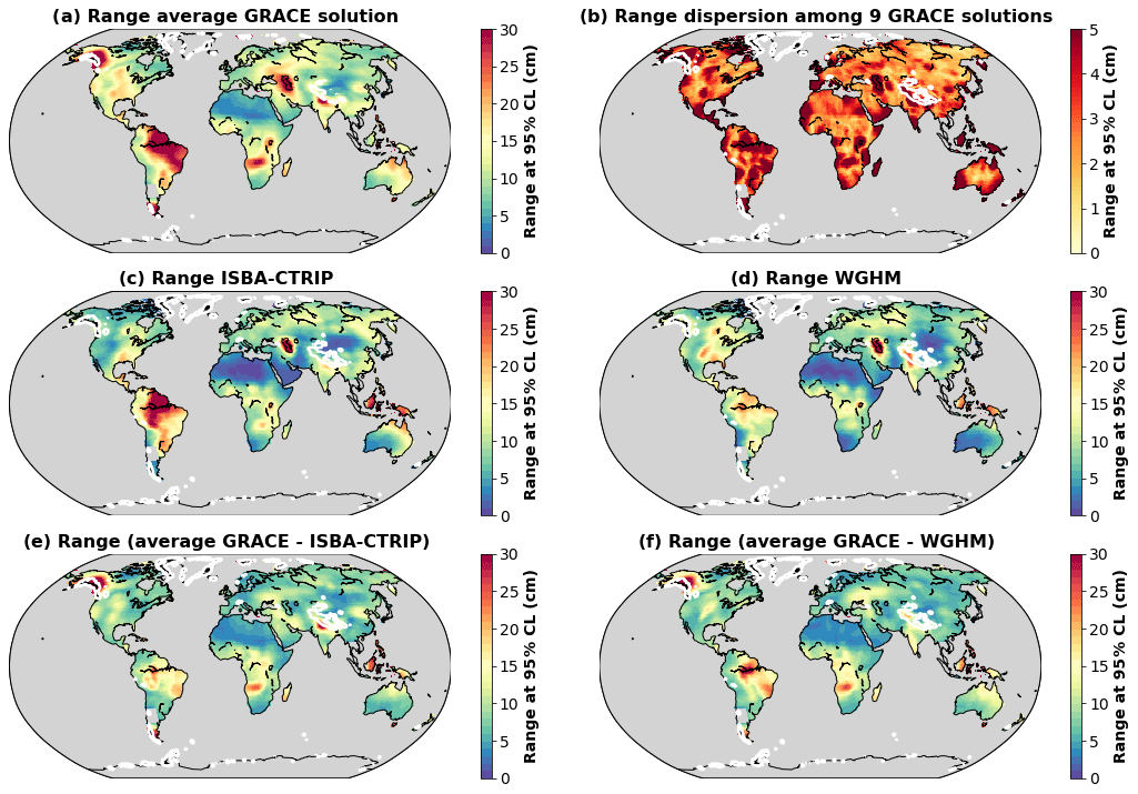
Figure 1Comparison of TWS anomalies estimated from an ensemble of nine GRACE solutions and two global hydrological models. The amplitude of the non-seasonal TWS variability is expressed as the range at 95 % CL, calculated as the difference between the 97.5 and 2.5 percentiles of the TWS anomalies obtained in each grid cell over the entire study period. TWS predictions from global hydrological models should not be compared with GRACE data around glaciers, identified by white contours. (a) Range of TWS anomalies estimated as the average of nine GRACE solutions. (b) Dispersion of the range of TWS anomalies among nine GRACE solutions. Range of TWS anomalies estimated with ISBA-CTRIP (c) and WGHM (d). Range of residual TWS anomalies estimated as the difference between the average of nine GRACE solutions and ISBA-CTRIP (e) or WGHM (f).
3.1 Comparison of observed and predicted TWS anomalies
TWS anomalies are globally lower in hydrological models than in GRACE solutions, leaving large residuals in GRACE satellite data (Fig. 1). The underestimation of TWS anomalies is more acute with WGHM (Fig. 1d) than with ISBA (Fig. 1c). Significant (>5 cm) residual TWS anomalies (Fig. 1e and f) are observed in South America (Amazon, Orinoco, São Francisco and Paraná River basins), Africa (Congo and Zambezi basins), Australia (northern part of the continent), Eurasia (India, North European Plain, Ural Mountains, Siberian Plateau) and North America (Colorado Plateau, Rocky Mountains). All GRACE solutions are remarkably consistent with each other, which is evidenced by small dispersion values (Fig. 1b). The amplitude of non-seasonal TWS signals is very similar in mascons and spherical harmonic solutions, which is generally larger than in global hydrological models (Supplement Figs. S2.1 and S2.2).
In most regions of the world, the differences between GRACE and global hydrological models (Fig. 1e and f) are much larger than the dispersion between the different GRACE solutions. Indeed, the residual TWS anomalies are significantly larger (5th, 50th and 95th percentiles of the rms of residual TWS anomalies at 4, 8 and 20 cm) than the uncertainty on GRACE data estimated by the dispersion among the nine solutions (5th, 50th and 95th percentiles of the standard deviation between the nine GRACE solutions at 1, 3 and 13 cm). The largest (≥5 cm) dispersion values are observed in coastal and mountainous regions or in regions with very large (≥20 cm) residuals (Fig. 1b). Larger sources of errors are indeed expected near the coast in GRACE measurements due to leakage errors, making the interpretation of residual signals difficult in islands such as Madagascar or the Indonesian archipelago. Similarly significant ice melt from glaciers occurs in mountainous regions such as the Alaska or Tibetan Plateau, which is monitored by GRACE but not simulated by global hydrological models, leaving large TWS residuals (30 cm) around glaciers. Global hydrological models should therefore not be compared with GRACE around glaciers, whose limits have been determined with the sixth version of the Randolph Glacier Inventory (RGI Consortium, 2017) identified with white contours in Fig. 1.
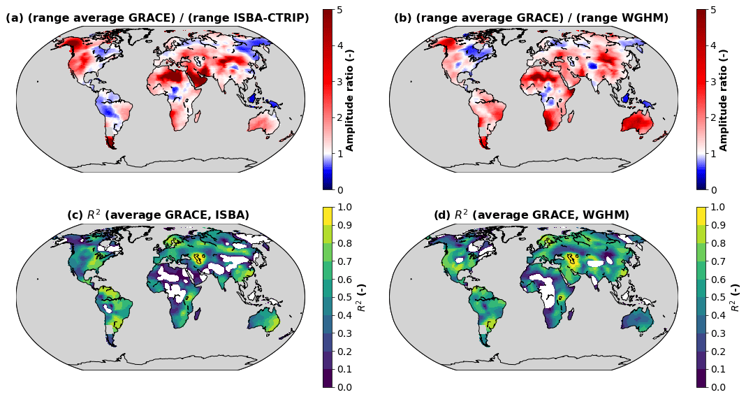
Figure 2Range ratios between the average GRACE solution and the hydrological models ISBA-CTRIP (a) and WGHM (b). Determination coefficients between the average GRACE solution and the hydrological models ISBA-CTRIP (c) and WGHM (d). Regions where the coefficient of determination is negative are shown in white.
To be able to differentiate a systematic underestimation of TWS anomalies from singular differences in the spatial and temporal variability, we computed the range ratio between the average GRACE solution and each hydrological model. For most regions of the world (Fig. 2a and b), the range of TWS anomalies is larger for GRACE than for ISBA-CTRIP or WGHM, except in east Canada (Ontario, Quebec, Newfoundland), north Asia (east Siberia, Ob River, Finland/north-west Russia) and central Africa (Cameroon, Gabon, Congo). In these regions, the coefficient of determination (R2) between the GRACE and the hydrological models is typically negative (Fig. 2c and d), indicating that the variance of the residuals is larger than the variance of GRACE data. The global hydrological models ISBA-CTRIP and WGHM are therefore not able to predict the TWS variability estimated from GRACE satellite data in these regions.
The large residuals observed with ISBA-CTRIP in the north-west of South America (Fig. 1e) are due to differences in the spatial and temporal variability of observed and predicted TWS changes. The range of TWS variations is indeed larger for ISBA-CTRIP than for GRACE in this region. R2 values are relatively high (0.5–0.9) in the north of the Amazon, indicating important similarities between GRACE and ISBA-CTRIP. Conversely, R2 values are very low (<0.3) in the south of the Amazon, indicating significant differences between GRACE and ISBA-CTRIP.
The range of TWS anomalies is smaller for hydrological models than for GRACE over most of the study area (76 % for ISBA-CTRIP and 83 % for WGHM). TWS anomalies predicted by hydrological models are underestimated by at least 50 % over almost half of the study area (40 % for ISBA-CTRIP and 49 % for WGHM). TWS anomalies are at least 2 times smaller than GRACE for 22 % of the study area for ISBA-CTRIP and 25 % for WGHM. The largest range ratios (>5) are reached across deserts (Sahara, Arabian Peninsula, Gobi Desert) and glaciers (Alaska, Patagonia, Himalaya). Such differences are due to numerical artefacts (denominator near zero) and non-hydrological signals (ice melting) observed by GRACE. Very large range ratios (2–4) are also observed for ISBA-CTRIP across the United States (Great Plains aquifer) and the north of India because of significant anthropogenic influences in these regions, with a potential contribution of glaciers across the north of India (Blazquez, 2020). Large-range ratios (from 2 to 5) are reached in tropical and subtropical regions of the Southern Hemisphere (Africa, South America, Australia) for WGHM.
Over more than half of the study area (61 % for ISBA-CTRIP and 53 % for WGHM), global hydrological models explain a minor part (R2<0.5) of the variance of the TWS anomalies estimated with the average GRACE solution (Fig. 2c and d). By comparison with GRACE, WGHM is more performant in the Northern than Southern Hemisphere. Relatively large R2 values (>0.5) are reached in the United States, central and northern Europe, west and central Siberia, eastern Asia, north of India, the Caspian Sea, and the Arabian Peninsula (Fig. 2d). Large R2 values are also reached over most of South America (Fig. 2d). Lower R2 values (<0.5) are reached over most of the African and Australian continents and parts of the Northern (north Canada, central Asia, east Siberia, south India) Hemisphere (Fig. 2d). By comparison (Fig. 2c), ISBA-CTRIP is more performant (R2>0.5) in the Southern Hemisphere (north, central and east Australia; southern and eastern Africa; and South America except Peru, Bolivia and Patagonia) and parts of the Northern Hemisphere (eastern United States, south Canada, central and northern Europe, south of Siberia, Caspian Sea, south of India, east China). Lower R2 values (<0.5) are reached for ISBA-CTRIP in north Canada, west and central Africa, Arabian Peninsula, south and central Asia, and west Australia (Fig. 2c). Both models exhibit negative R2 values in central and Sahelian Africa, as well as in Quebec and Ontario (Fig. 2c and d). For ISBA-CTRIP, negative R2 coefficients are also reached in north Bolivia, Alaska, north of India and Siberia (south of Lena River). For WGHM, negative R2 coefficients are reached in the central United States and south India. These metrics indicate that for some regions of the world (not necessarily the same for both models), hydrological models are able to capture a large part of the TWS variability estimated from GRACE but that, overall, significant differences exist between global hydrological models and GRACE satellite data.
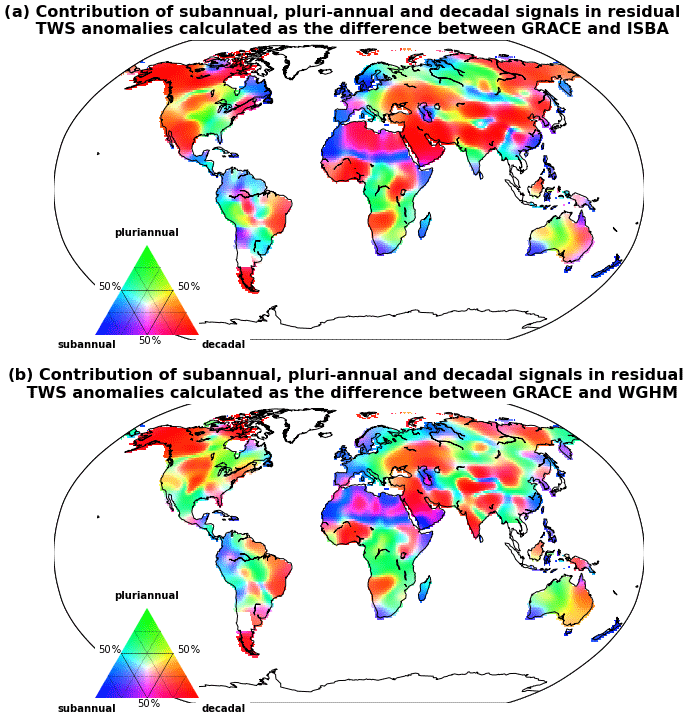
Figure 3Characteristic timescales in residual TWS anomalies calculated as the differences between the average GRACE solution and ISBA-CTRIP (a) or WGHM (b). Subannual, pluri-annual and decadal contributions have been computed with high-pass (cut-off period at 1.5 years), band-pass (cut-off periods at 1.5 and 10 years) and low-pass (cut-off period at 10 years) filters respectively. The percentage of variance explained by one contribution has been calculated as the coefficient of determination with respect to the full residual signal.
3.2 Characteristic timescales of residual TWS anomalies
The differences in TWS anomalies estimated from GRACE and global hydrological models (or residual TWS anomalies) are largely dominated by pluri-annual and decadal signals (Fig. 3). Residual TWS anomalies have been separated into subannual, pluri-annual and decadal contributions using high-pass (cut-off period at 1.5 years), band-pass (cut-off periods at 1.5 and 10 years) and low-pass (cut-off period at 10 years) filters respectively. The percentage of variance explained by each contribution has been calculated as R2 values and reported in Maxwell's colour triangle (Fig. 3). Residual TWS anomalies are dominated by decadal signals over a large part of the study area (51 % with ISBA-CTRIP and 40 % with WGHM), including Alaska; west Canada; the Brazilian highlands (São Francisco and Paraná River basins); Patagonia; west (Niger and Volta River basins) and southern Africa (Okavango and Zambezi River basins); parts of west (Arabic Peninsula, Caspian Sea drainage area, Tigris–Euphrates, Dnieper, Volga and Don River basins), central (Tibetan Plateau and Tarim, Ganges and Brahmaputra River basins) and north (Yenisei and Lena River basins) Asia; and east Australia. When calculating the residuals with ISBA-CTRIP, large decadal signals are also observed across north-west America (Sierra Madre, Sierra Nevada, Great Basin, Rocky Mountains) and the north of India (Indus River basin).
Pluri-annual signals are prevalent in residual TWS anomalies across central Africa, western Australia, Siberia (Ob and Yenisei), eastern Europe, north-east America (Great Lakes) and the southwest of the Amazon basin. Subannual signals are prevalent in regions with tenuous TWS variability (i.e. Sahara, southern Africa, southwest Australia), likely pointing out the remaining level of noise in GRACE data (Fig. 1b). Regions with large (≥10 cm) residual TWS anomalies (Fig. 1e) are systematically dominated by pluri-annual to decadal contributions (Fig. 3). On the other hand, regions with very small (<2 cm) residual TWS anomalies, such as the Sahara, are dominated by subannual and decadal contributions (Fig. 3). As no significant geophysical signal is expected in such regions, this can be interpreted as the spectral content of the noise, including both a high-frequency and low-frequency component.
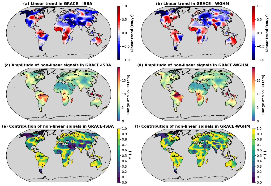
Figure 4(a) Linear trends in residual TWS anomalies calculated as the difference between the average GRACE solution and ISBA-CTRIP. (b) Same as (a) with WGHM. (c) Amplitude of non-linear signals in residual TWS anomalies calculated as the difference between the average GRACE solution and ISBA-CTRIP. The amplitude is calculated as the difference between the 97.5 and 2.5 percentiles. (d) Same as (c) with WGHM. (e) Coefficient of determination calculated for non-linear signals with respect to TWS anomalies calculated as the difference between the average GRACE solution and ISBA-CTRIP. (f) Same as (e) with WGHM.
Residual TWS anomalies are dominated by pluri-annual and decadal changes in the TWS, including linear trends and non-linear signals (Fig. 4). Though significant linear trends are detected (±1 cm yr−1), residual TWS anomalies are mainly due to non-linear variability in the TWS (Fig. 4). Apart from glaciers, significant trends in TWS residuals are observed in west (Niger) and southern (Okavango and Zambezi) Africa, north-east Australia, south Asia (mostly the north of India, especially when using ISBA-CTRIP), north-west America (ISBA-CTRIP only) and the central United States (mainly WGHM). Part of the residual TWS trends observed with ISBA-CTRIP in north-west America (Sect. 4.6) and south Asia (Sect. 4.7) are likely due to anthropogenic influences, including groundwater abstractions primarily used for irrigation. In other regions of the world, residual trends in TWS are likely related to climate variability (precipitation excess/deficit which may be associated with the alternance of wet/dry phases of natural climate modes such as ENSO in southern Africa and north-east Australia) or land-use changes (west Africa). In most regions of the world (72 % of the study area for ISBA-CTRIP and 83 % for WGHM), the residual variability in TWS cannot be explained by a linear trend and involves significant variability at interannual and decadal timescales (Fig. 4c to f).
To better characterise and understand the nature of residuals, TWS anomalies estimated from GRACE and global hydrological models have been averaged over large regions of the world and compared to in situ and satellite precipitation. In the following, we discuss regional TWS anomalies where the largest residuals are observed around the Central Amazon Corridor, the upper São Francisco River, the Zambezi and Okavango rivers, the Congo River, the north of Australia, the Ogallala aquifer in central United States, the north of the Black Sea and the Northern Plains of India (see map in Fig. B1 in Appendix B). For each of these regions, all the solutions of the GRACE ensemble (three mascon and six spherical harmonic solutions) detect slow changes in TWS, which indicates high confidence in these observations. Larger differences occur between ISBA-CTRIP and WGHM, and both models systematically underestimate the pluri-annual and decadal changes in TWS captured by GRACE. Part of these differences may be attributed to common sources of errors in GRACE-based TWS estimates, including errors in background models (for example, the atmospheric circulation model) and post-processing choices (for example, the GIA model). However, errors in the atmospheric model (GAA from AOD1B, based on ERA5) would be associated with fast changes in TWS, while errors in the GIA model (ICE6G-D) would be characterised by linear trends over the GRACE period. Here, the largest differences between GRACE and global hydrological models occur at pluri-annual and decadal timescales and are generally well correlated with precipitation. A large part of the differences between GRACE and global hydrological models are therefore likely to be climate-related and at least partially due to inaccurate predictions of global hydrological models. Similar regional analyses have been done for the 40 largest river basins of the world with comparable results (Figs. S3.1 to S3.41).
4.1 Central Amazon Corridor
4.1.1 Study area
The Central Amazon Corridor (1∘ N–7∘ S and 75–50∘ W) surrounds the Solimões/Amazon mainstream river and the downstream parts of its main tributaries, including the Japura, Jurua, Purus, Negro, Madeira, Trombetas, Tapajos and Xingu rivers. Those large rivers exhibit a monomodal flood pulse lasting several months, flooding an extensive lowland area, largely covered by forests (e.g. Junk, 1997; Melack and Coe, 2021). The extension of the flooded area varies from 100 000 to 600 000 km2 in the Amazon basin (e.g. Fleishmann et al., 2022), in phase with water level variations in rivers that can reach up to 15 m annually (e.g. Birkett et al., 2002; Alsdorf et al., 2007; Frappart et al., 2012; Da Silva et al., 2012), with significant interannual variability (e.g. Fassoni-Andrade et al., 2021). Heterogeneous soils distributions, including Ferralsols, Plinthosols and Gleysols (e.g. Quesada et al., 2011), lie over unconsolidated sedimentary rocks, alluvial deposits and consolidated sedimentary rocks with relatively homogeneous hydraulic properties (e.g. Gleeson et al., 2011; Fan et al., 2013). Across the central Amazon lowlands, the groundwater table fluctuates by several metres (Pfeffer et al., 2014), corresponding to groundwater storage changes of several tens of centimetres (Frappart et al., 2019), which constitutes a large part of the TWS changes observed by GRACE (Frappart et al., 2019).
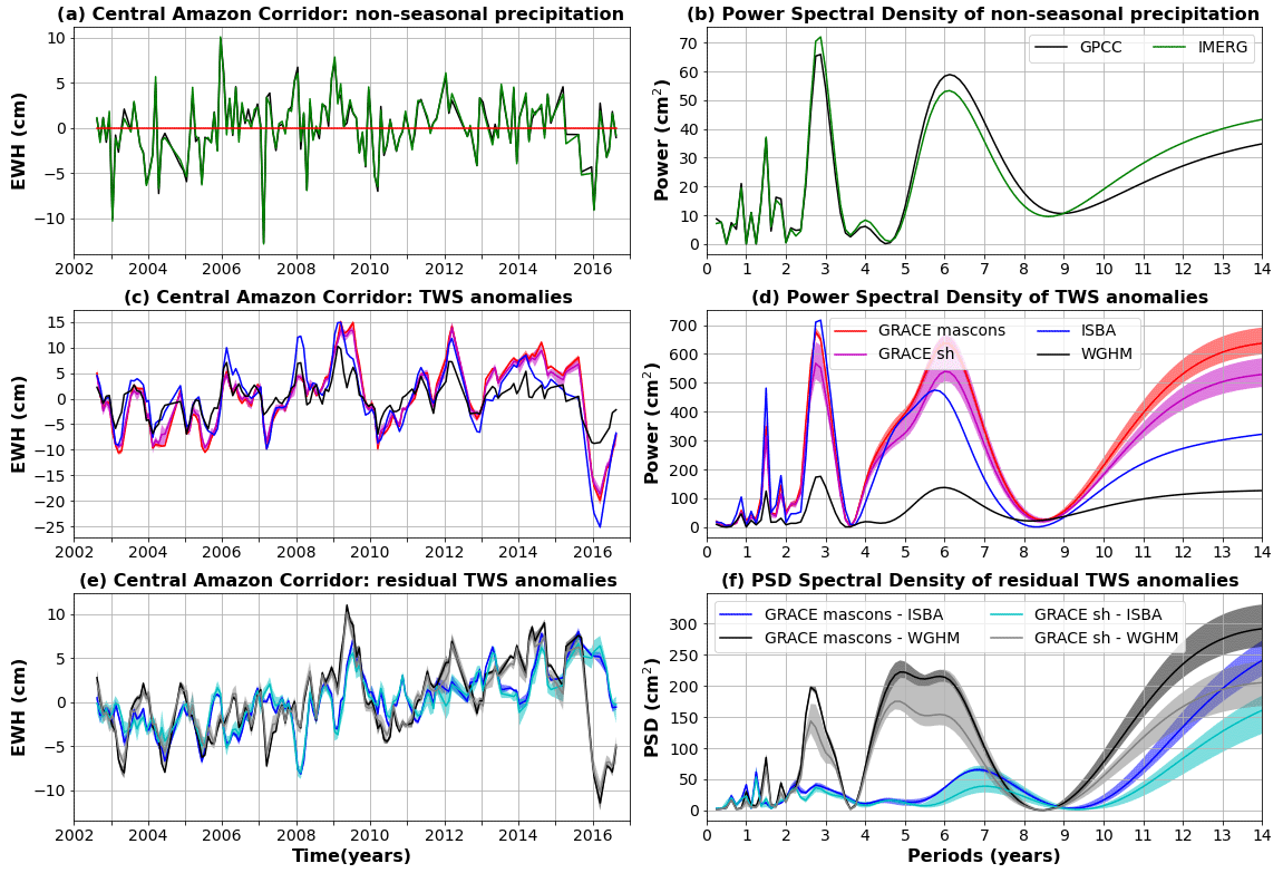
Figure 5Comparison of TWS and precipitation anomalies averaged over the Central Amazon Corridor (box A in Fig. B1 in Appendix B). (a) Average precipitation anomalies for the GPCC (gauge-based) and IMERG (satellite-based) products. (b) Power spectral density (PSD) of average precipitation anomalies. (c) TWS anomalies average over the central Amazon for two global hydrological models (ISBA-CTRIP in blue and WGHM in black) and nine GRACE solutions (mascons in red, spherical harmonic in magenta). The solid line corresponds to the average of the sub-ensemble and the shaded area to the minimum to maximum envelope. (d) PSD of the averaged TWS anomalies shown in (c). (e) Residual TWS anomalies averaged over the Central Amazon Corridor and calculated as the difference between GRACE and ISBA-CTRIP (blue when the difference is calculated with mascons and cyan with spherical harmonics) or WGHM (black when the difference is calculated with mascons and grey with spherical harmonics).
4.1.2 Comparison of global hydrological models with GRACE
Over the central Amazon region (Fig. 5), TWS anomalies predicted by global hydrological models agree well with GRACE observations, with very large Pearson coefficients reached for both ISBA-CTRIP (R=0.90) and WGHM (R=0.86). The amplitudes of TWS anomalies predicted with ISBA-CTRIP match GRACE solutions closely, while WGHM tends to underestimate the TWS variability at interannual and decadal timescales, which is likely due to a more accurate representation of the floodplains and their interactions with the atmosphere, soil and aquifer with ISBA-CTRIP than WGHM (Fig. 5d). Interannual variability occurs in the precipitation as well (Fig 5a and b), with significant correlation with GRACE (R=0.54), ISBA (R=0.59) and WGHM (R=0.64) and a phase lag of 1 month. Despite good performances for both models (especially ISBA-CTRIP), significant residual signals remain in TWS anomalies after correction of hydrological effects, consisting mostly of an increasing trend with ISBA-CTRIP, with significant interannual variability superimposed for WGHM. The residual TWS changes corrected with WGHM are still significantly correlated with precipitation (R=0.48) with a phase lag of 4 months. No significant correlation can be found between the residual TWS anomalies calculated with ISBA and precipitation anomalies (maximum R value of 0.22 with a time lag of 14 months), though significant decadal and pluri-decadal variability can be observed in GPCC precipitation records, which may explain a residual trend in TWS (∼5 mm yr−1).
Residual TWS anomalies may be due to inaccurately modelled water storage variations in any reservoir from the surface to the aquifer. The largest residual TWS variations are observed along the downstream part of the Solimões, at the confluences with the Purus and the Rio Negro, which is a region that is largely covered by floodplains (e.g. Fleishmann et al., 2022) and dominated by changes in surface water storage (Frappart et al., 2019). The long timescales associated with the residuals and increasing time lags with precipitation suggest however a significant contribution from groundwater storage fluctuations, which are insufficiently constrained in global hydrological models (e.g. Decharme et al., 2019; Scanlon et al., 2018, 2019). Large floodplains may indeed delay the water transport for several months (e.g. Prigent et al., 2020), through storage and percolation from the surface towards the aquifer (e.g. Lesack and Melack, 1995; Bonnet et al., 2008; Frappart et al., 2019). Groundwater stores excess water during wet periods and sustains rivers and floodplains during low-water periods (e.g. Lesack, 1993). Groundwater systems have also been shown to convey seasonal anomalies (for example, droughts) for several years at local (e.g. Tomasella et al., 2008) and regional (Pfeffer et al., 2014) scales. Such memory effects may be underestimated by global hydrological models, which would result in much faster variations of the TWS.
4.2 Upper São Francisco
4.2.1 Study area
The São Francisco River, located in north-east Brazil, is 3200 km long and drains an area of about 630 000 km2. Hydroelectric dams located along the São Francisco provide about 70 % of north-east Brazil's electricity, including the Três Marias, Sobradinho and Luíz Gonzaga (Itaparica) reservoirs with respective volumes of 15 278, 28 669 and 3549 hm3. Significant decreases in the river flow during the 1980–2015 period have been attributed to increased groundwater withdrawals sustaining irrigated agriculture and decreasing the groundwater contributions to streamflow (i.e. baseflow) (Lucas et al., 2020). As a result of a prolonged drought lasting from 2002 to 2017 (Freitas et al., 2021), the São Francisco hydroelectric plants only provided a minor part (from 18 % to 42 % depending on the year) of the total electricity demand, which was sustained by increased fossil fuel consumption (de Jong et al., 2018). A decrease in TWS was also observed from 2012 to the end of the GRACE mission (mid-2017) across the São Francisco coincident with the observed rainfall deficit (Ndehedehe and Ferreira, 2020), allowing the impact of prolonged droughts on the water supply in a vulnerable region to be better quantified (Paredes-Trejo et al., 2021).
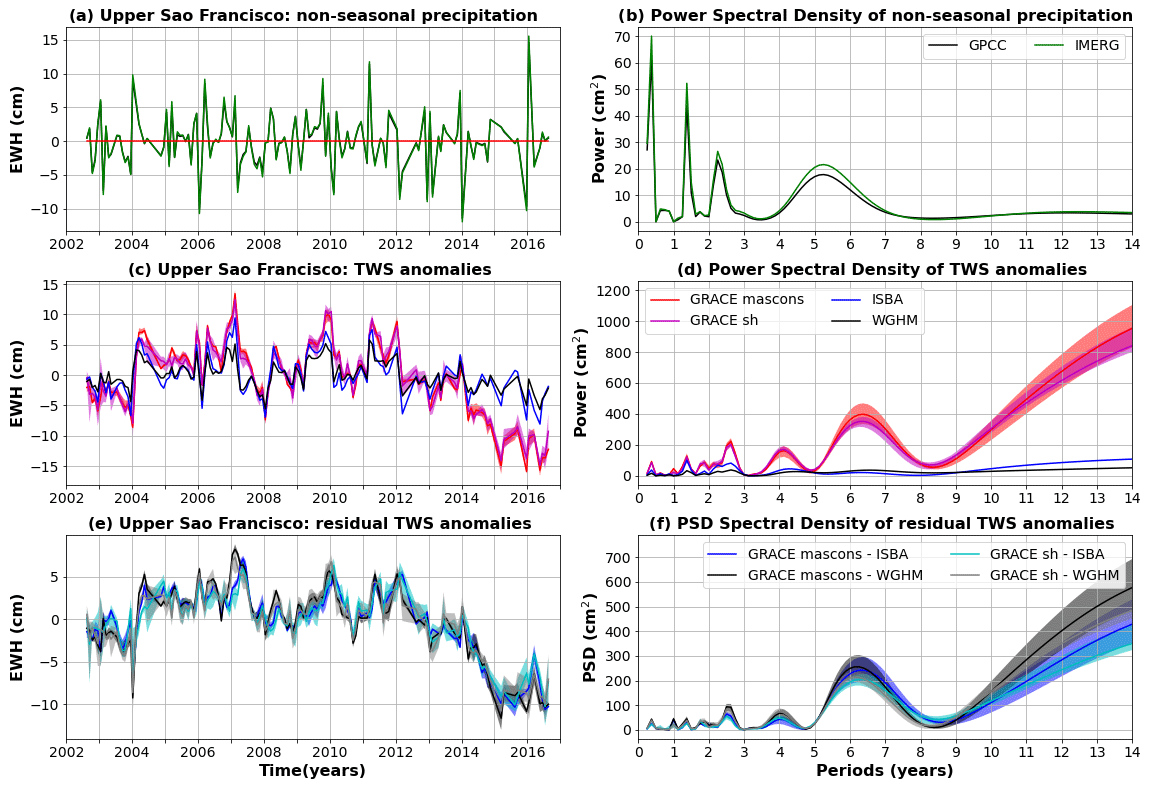
4.2.2 Comparison of global hydrological models with GRACE
Over the upper São Francisco region (Fig. 6), TWS anomalies predicted with global hydrological models are well correlated with GRACE data on a year-to-year basis (R=0.79 for ISBA and R=0.81 for WGHM). The times of the minimum and maximum TWS anomalies are well picked up by satellite gravity observations and models, though the amplitude of TWS anomalies is underestimated by global hydrological models. All nine GRACE solutions exhibit interannual and decadal variability in TWS, which is absent in both global hydrological models. In particular, GRACE monitors a drop in terrestrial water storage from 2012 to 2016 (Fig. 6b), corresponding to 4 years of consecutive deficit in precipitation (Fig. 6a), which is not picked up by global hydrological models. As a consequence, residual TWS anomalies (Fig. 6e), characterised by prominent interannual and decadal signals (Fig. 6f), reach 10–20 cm in the São Francisco region. TWS anomalies predicted by hydrological models are relatively well correlated with precipitation (R=0.6 for ISBA and 0.52 for WGHM) with a time lag of 1 month, while the correlation with GRACE TWS anomalies is more marginal (R=0.39 with a time lag of 1 month). Residual TWS anomalies are also only marginally correlated with precipitation (R=0.29 for GRACE-WGHM and 0.33 for GRACE-ISBA), with a time lag of 3 months.
These results tend to show that global hydrological models reproduce the year-to-year variability of TWS anomalies across the São Francisco quite well (especially in term of occurrence of a wet/dry anomaly, as the amplitudes of the anomalies may be underestimated) but struggle to predict slower hydrological processes characterised by interannual and decadal timescales.
4.3 Zambezi–Okavango
4.3.1 Study area
The Zambezi River basin, located in south tropical Africa, drains an area of 1.4×10⁶ km2 connecting Angola (18.3 %), Namibia (1.2 %), Botswana (2.8 %), Zambia (40.7 %), Zimbabwe (15.9 %), Malawi (7.7 %), Tanzania (2.0 %) and Mozambique (11.4 %) (Vörösmarty and Moore, 1991). It encompasses humid, semi-arid and arid regions dominated by seasonal rainfall patterns associated with the Intertropical Convergence Zone (ITCZ), with a wet season spanning October to April and a dry season spanning May to September (Lowmann et al., 2018). The Zambezi basin harbours very large wetland areas and lakes, whose extension considerably varies with precipitation at seasonal and interannual timescales (Hugues et al., 2020). Significant interannual variability in the precipitation and TWS has been detected over the Zambezi and Okavango regions and attributed to several climate modes, including the Pacific Decadal Oscillation, Atlantic Multidecadal Oscillation and El Niño–Southern Oscillation (Pfeffer et al., 2021).
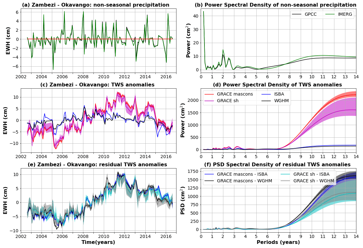
Figure 7Same as Fig. 5 but for the Zambezi and Okavango rivers (box C in Fig. B1 in Appendix B).
4.3.2 Comparison of global hydrological models with GRACE
Across the Zambezi and Okavango region (Fig. 7), TWS anomalies are well correlated with precipitation (R=0.62 and 0.49 with a time lag of 1 month for ISBA-CTRIP and WGHM). Positive (respectively negative) precipitation anomalies correspond to a local maximum (respectively minimum) in TWS. This year-to-year variability is consistent between GRACE and global hydrological models, as evidenced by a Pearson correlation coefficient of 0.60 between GRACE and ISBA-CTRIP and 0.63 between the GRACE and WGHM. However, the TWS anomalies estimated from GRACE exhibit a strong decadal oscillation, with a minimum in 2005/2006 and a maximum in 2011/2012 that is not picked up by hydrological models, leaving a very strong (20 cm in amplitude) decadal anomaly in the residuals TWS. Though the residual TWS anomalies are poorly correlated with the precipitation anomaly (R=0.23 and 0.25 with a phase lag of 28 and 40 months for GRACE–ISBA and GRACE–WGHM respectively), they are strongly related to the accumulated precipitation anomalies, also exhibiting a strong decadal anomaly with a minimum in 2005/2006 and a maximum in 2011/2012.
The TWS residuals can be reduced locally by up to 50 % in the Zambezi region by applying an empirical model based on climate modes, as formulated by Pfeffer et al. (2021). The main modes of variability found in the TWS residuals are the Pacific Decadal Oscillation and the Atlantic Multidecadal Oscillation.
4.4 Congo
4.4.1 Study area
The Congo basin is the second-largest river basin in the world, with a drainage area of km2 and an average annual discharge of ∼40 500 m3 s−1 (Laraque et al., 2020). Despite its importance, the Congo River basin is scarcely studied (Alsdorf et al., 2016), though a growing interest has arisen over the past decade, substantially due to advances in satellite hydrology (e.g. Papa et al., 2022; Paris et al., 2022; Schumann et al., 2022). With an average rainfall around 1500 mm−1, the Congo basin benefits from a humid tropical climate with a complex seasonal migration of rainfall across the basin with a first maximum in November–December and a second peak in April–May (Alsdorf et al., 2016), leading to a bimodal river discharge (Kitambo et al., 2022). The “Cuvette centrale” is a topographic depression located at the centre of the basin, harbouring wetlands covered by rainforests permanently or periodically flooded (Becker et al., 2018). The Congo floodplain hydrodynamics are disconnected from the main river, with much less variability observed throughout the year (Alsdorf et al., 2016). The Congo River basin hosts a large complex fractured sedimentary aquifer, with relatively low storage but high recharge rates (Scanlon et al., 2022). Very little is known about the groundwater storage variability, though comparisons of satellite estimations of the surface water storage with the total terrestrial water storage changes from GRACE suggest that most (∼90 % at annual timescales) of the variability in water storage occurs under the surface (Becker et al., 2018).
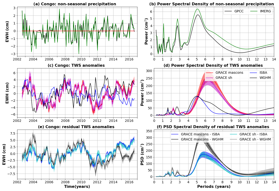
4.4.2 Comparison of global hydrological models with GRACE
Non-seasonal TWS anomalies are very different over the Congo basin depending on the method of estimation considered (Fig. 8). All nine GRACE solutions are consistent with each other but differ from both global hydrological models that also exhibit large discrepancies with each other (Fig. 8). The correlations of TWS anomalies with precipitation are also marginal (maximum correlation of 0.5 with WGHM). All nine GRACE solutions exhibit a 6-year cycle, in phase with accumulated precipitation with local minima in 2006 and 2012 and local maxima in 2003, 2009 and 2015 (Fig. 8). Slow changes in TWS observed with GRACE are not predicted by hydrological models, leaving large residuals in TWS characterised by a ∼6-year cycle (Fig. 8).
Significant power is found in multi-decadal precipitation time series at similar periods, ranging from 5 to 8 years (Laraque et al., 2020), as well as in discharge times series at 7.5 and 13.5 years (Labat et al., 2005). The variability of the TWS cannot be explained by major climate modes over the Congo River basin, except for the PDO, which may slightly influence the TWS variability in the north of the Congo River (Pfeffer et al., 2022). The variability in river discharge has been found to be temporarily consistent with NAO at 7.5 years (from the 1970s to the 1990s) and 35 years (from the 1940s to the 1990s) (Labat et al., 2005). Part of the inaccuracies in global hydrological models may be due to (i) the scarcity of in situ data available to constrain precipitation (Fig. 2 in Laraque et al., 2020); (ii) errors in runoff and evapotranspiration fluxes; or (iii) unresolved underground processes, including preferential flow along faults (Fig. 1 in Garzanti et al., 2019).
4.5 North Australia
4.5.1 Study area
The climate of north Australia is characterised by a wet season lasting from November to April, subject to intense thunderstorms and cyclones, with virtually no precipitation during the remainder of the year (Smith et al., 2008). Annual streamflow is highly dominated by monsoon rainfall, with dry-season flows fed by groundwater discharge that may stop for several months for a large number of rivers (Petheram et al., 2008; Smerdon et al., 2012). Groundwater plays an essential role in north Australia as it sustains rivers and vegetation, through baseflow and water uptake for plant transpiration (Lamontagne et al., 2005; O'Grady et al., 2006). Significant interannual variability, principally related to ENSO in the north of the continent, has been observed in rainfall (Cai et al., 2001; Sharmila and Hendon, 2020), river discharge (Chiew et al., 1998; Ward et al., 2010) and terrestrial water storage (Xie et al., 2019). During the GRACE era, Australia encountered a prolonged drought from 2002 to 2009, sometimes referred to as the “millennium drought” or “big dry”, immediately followed by intensely wet conditions in 2010–2011 (the “big wet” associated with La Nina) and a sustained drought, leading to another dry El Niño event in 2015 (Fig. 3 in Xie et al., 2019, and Fig. 9 in the present paper). Three major climate modes (ENSO, IOD and SAM) are necessary to explain the water storage variability across Australia, but the northern part of the country is dominated by ENSO (Xie et al., 2019).
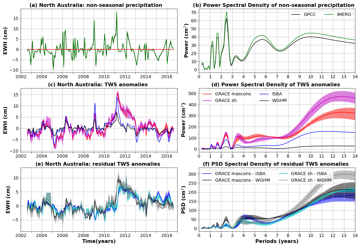
4.5.2 Comparison of global hydrological models with GRACE
Across north Australia (Fig. 9), TWS anomalies predicted by global hydrological models are well correlated with precipitation (R=0.73 and 0.67 with a phase lag of 1 month for ISBA and WGHM) and TWS anomalies estimated with GRACE (R=0.76 and 0.71 with ISBA and WGHM respectively). The amplitude of extreme events (for example La Niña in 2011) from ISBA matches GRACE estimates, while WGHM tends to underestimate the response of TWS to both dry (2005) and wet (2011) events (Fig. 9). The main difference between TWS estimations from global hydrological models and GRACE solutions is the pace at which TWS returns to average conditions after a wet/dry event (Fig. 9). For example, after the flooding events associated with La Niña 2011, all nine GRACE solutions estimate a slow decrease in the TWS returning to average conditions in about two years (Fig. 9). On the other hand, both global hydrological models predict a sharp decrease in the TWS returning to average conditions in about 6 months (Fig. 9). As a consequence, a positive TWS anomaly remains in the residuals after La Niña (Fig. 9), accounting for the differences in the rate of change of TWS.
These results are consistent with the findings of Yang et al. (2020), who found that except for the CLM-4.5 model, hydrological models underestimated the GRACE-derived TWS trends across Australia, due to inaccurately modelled contributions from soil moisture and groundwater storage. Similarly, TWS anomalies from GRACE were found to be a better link between vegetation change and climate variability than precipitation (Xie et al., 2019) because they convey more information about water availability in the soils and aquifers, especially when associated with SMOS (Soil Moisture and Salinity) measurements (Tian et al., 2019).
4.6 Central United States: Ogallala aquifer
4.6.1 Study area
The Ogallala, or High Plains, aquifer covers a surface area of about 450 000 km2 across eight states in the central United States, including parts of Colorado, Kansas, Nebraska, New Mexico, Oklahoma, South Dakota, Texas and Wyoming. The Ogallala aquifer region supports about 20 % of the wheat, corn and cotton production in the United States (Houston et al., 2013). Groundwater abstractions for irrigation began in Texas in the 1930s (Luckey et al., 1981) and exceeded recharge over much of the central and southern parts of aquifer in the 1950s (Luckey and Becker, 1999), resulting in substantial decline of the groundwater table in the Southern and Central High Plains, while the Northern High Plains stayed in balance or replenished (Haacker et al., 2016). At current depletion rates, a large part of irrigation (about 30 %) may not be supported in the coming decades (Scanlon et al., 2012b; Haacker et al., 2016; Steward and Allen, 2016; Deines et al., 2020).
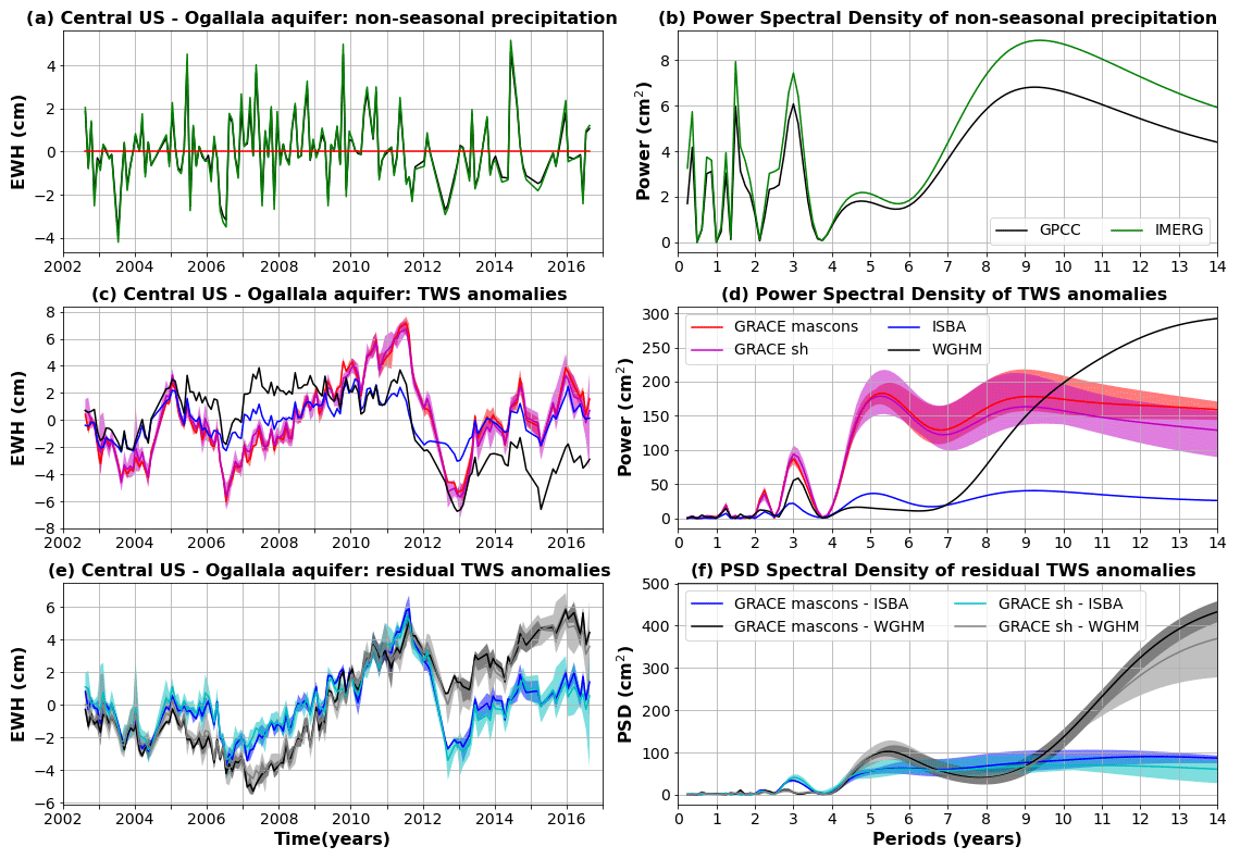
Figure 10Same as Fig. 5 but for the central United States – Ogallala aquifer region (box F in Fig. B1 in Appendix B).
4.6.2 Comparison of global hydrological models with GRACE
In the Ogallala aquifer region, all GRACE solutions exhibit a series of upwards and downwards trends in TWS with a regular increase from mid-2006 to mid-2011 and a sharp decrease in TWS from mid-2011 to 2013, followed by another increase in TWS from early 2013 to 2016 (Fig. 10). This pattern is linked with precipitation anomalies that were mainly in excess over 2006–2011 and in deficit over 2011/2013 and oscillated around average values over 2013–2016, with a remarkably rainy year in 2014 (Fig. 10). This succession of opposite trends is not predicted by global hydrological models (Fig. 10). WGHM does predict a sharp decrease in TWS from mid-2011 to 2013 but fails to predict the increase in TWS during 2006–2011 in spite of abundant precipitation (Fig. 10).
Such differences might be explained by an overestimation of water abstractions by WGHM, which would result in almost constant TWS changes, while precipitation, and subsequent aquifer recharge, is increasing. This assumption is supported by the work of Rateb et al. (2020), showing that global hydrological models such as WGHM or PCR-GLOBWB tend to overestimate groundwater depletion due to human intervention in the region. Good agreement is found between GRACE and in situ observations of the groundwater table, though large uncertainties affect (i) the decomposition of the GRACE-based TWS anomalies into individual water reservoirs (Brookfield et al., 2018) and (ii) the estimation of hydraulic parameters (i.e. conductivity and specific yield), allowing for the conversion of groundwater level variations to groundwater storage variations (Seyoum and Milewski, 2016). For the Ogallala aquifer region, GRACE data may help to characterise insufficiently well constrained parameters of WGHM, such as hydraulic parameters (i.e. conductivity, specific yield), or parameters of the water use model, such as irrigation efficiencies. In its current stage, the ISBA-CTRIP model is not adapted to estimate TWS changes in heavily managed regions because it does not take irrigation into account.
4.7 North of India
4.7.1 Study area
The north of India hosts the Indus, Ganges and Brahmaputra River basins, with an average annual rainfall of 545, 1088 and 2323 mm yr−1 respectively (e.g. Bhanja et al., 2016). The average population density ranges from 26–250 persons per km2 in the north-west of India to over 1000 persons per km2 in the north-east of India (Dangar et al., 2021). India is the largest groundwater user in the world, with an annual withdrawal of 230 km3 for irrigation, used essentially for rice, wheat, sugarcane, cotton and maize cultures (Mishra et al., 2018; Xie et al., 2019). High abstraction rates largely exceeding precipitation rates have been reported in north-west India, in particular in the Punjab region, leading to an aquifer depletion rate of about 1 m yr−1 (Mishra et al., 2018; Dangar et al., 2021). The Northern Plains of India are bordered by the Southern Tibetan Plateau, whose glaciers have been undergoing significant ice thinning due to increased temperatures (e.g. Hugonnet et al., 2021). Both contributions from land hydrology and glaciers may therefore influence GRACE-based TWS estimates in this region.
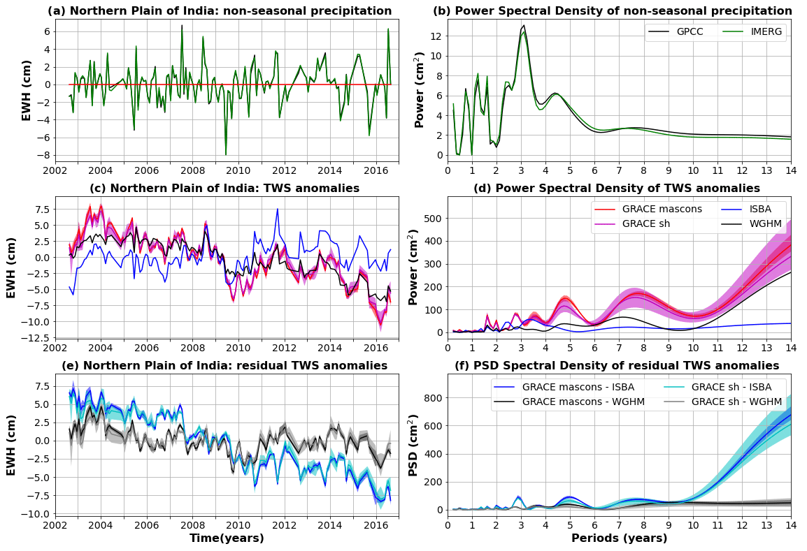
Figure 11Same as Fig. 5 but for the Northern Plains of India (box G in Fig. B1 in Appendix B).
4.7.2 Comparison of global hydrological models with GRACE
Because WGHM takes irrigation into account, predicted TWS anomalies closely match GRACE observations (R=0.96), leaving residuals of about ±2.5 cm (Fig. 11), which is about 4 to 6 times less than across the central Amazon (Fig. 5) or Zambezi (Fig. 7) regions. As expected in strongly anthropised regions, ISBA-CTRIP fails to recover the TWS changes estimated with GRACE, characterised by a clear decreasing trend ( mm yr−1) over 2002–2016 (Fig. 11), clearly due to groundwater abstractions for irrigation.
Besides, the superposition of several sources of mass redistributions (i.e. land hydrology and glaciers) may generate ambiguities in the interpretation of GRACE-based TWS estimates in the north of India (Blazquez, 2020). Groundwater abstractions were however found to be the dominant driver of water mass losses across northern India (e.g. Xiang et al., 2016). Numerous studies have reported a good agreement between in situ groundwater level measurements and GRACE TWS measurements in the north of India (e.g. Bhanja et al., 2016; Dangar et al., 2021). Detailed studies indicated that better model performances could be gained by adjustment of several parameters (water percolation rate, crop water stress, irrigation efficiency, soil evaporation compensation and groundwater recession) against GRACE data (Xie et al., 2019). Such information is critical to ensure the reliability of hydrological models across several regions. For example, the ISBA-CTRIP model exhibits better performances than WGHM when compared to GRACE across the southern Peninsular Plateau of India (Fig. 1) because of an overestimation of groundwater abstractions in WGHM, leading to spurious decreasing trends not observed by satellite gravity measurements (Fig. S4.1). An increase in TWS and in replenishment of groundwater resources has indeed been reported in south India from the analysis of GRACE and well data (e.g. Asoka et al., 2017; Bhanja et al., 2017).
4.8 North of the Black Sea
4.8.1 Study area
The Black Sea catchment hosts a population of 160 million people in 23 countries drained by major rivers including the Danube, Dniester, Dnieper, Don, Kuban, Sakarya and Kizirmak. The annual precipitation varies from less than 190 mm yr−1 at the north-east of the catchment (Russia) to more than 3000 mm yr−1 at the west (south Austria, Slovenia, Croatia) (Rouholahnejad et al., 2014, 2017). The annual average temperature varies from 2 to 7 ∘C at the north of the catchment (East European Plain at the border of Ukraine, Belarus and Russia), with a local minimum ( ∘C) in the Krasnodar region (southwest Russia), to over 15 ∘C at the south of the catchment (north of Turkey) (Rouholahnejad et al., 2014, 2017). Land use in the Black Sea catchment is dominated by agriculture (Rouholahnejad et al., 2014, 2017).
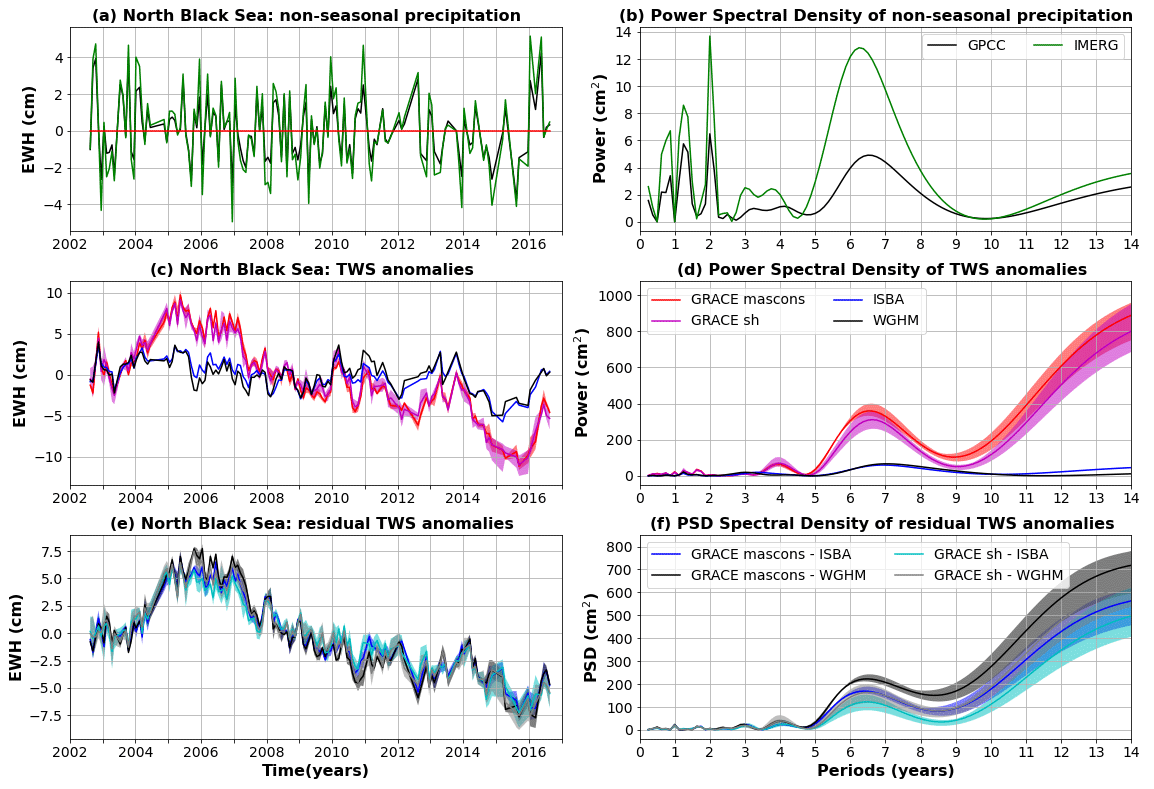
Figure 12Same as Fig. 5 but for the north of the Black Sea (box H in Fig. B1 in Appendix B).
4.8.2 Comparison of global hydrological models with GRACE
Large TWS residuals are observed in the north-east of the Black Sea catchment, in the East European Plain crossing Ukraine, Belarus and Russia (Fig. 12). Large (∼20 cm) TWS changes are observed by GRACE satellites in this region, characterised by a decreasing trend conjugated with significant interannual variability, with a peak at 6–7 years (Fig. 12). Such TWS changes are not predicted by hydrological models, leaving large (∼15 cm) TWS residuals, dominated by decadal and interannual variability (Fig. 12).
Due to rising temperatures, a generalised drop (10 %–15 %) in solid precipitation has been observed across the East European Plain, partially offset by liquid precipitation, except along the northern coast of the Black and Azov Sea (drop ∼10 %), the lower Volga River basin (drop ∼20 %) and the Dvina River basin further north (drop ∼25 %) (Kharmalov and Kireeva, 2020). A drop in summer precipitation, together with an increase in temperature, was observed at the north of the Black, Azov and Caspian Sea, generating severe drought conditions in the region (Kharmalov and Kireeva, 2020). Water scarcity has indeed become a critical concern, with increased water stress and decreased water availability, observed today and predicted to increase in the future (Rouholahnejad et al., 2014, 2017).
Over most (>75 %) continental areas, non-seasonal TWS anomalies are underestimated by the global hydrological models ISBA-CTRIP and WGHM when compared to GRACE solutions. While both hydrological models agree relatively well with GRACE observations on short timescales (i.e. typically less than 2 years), they systematically underestimate slower changes in TWS observed by GRACE satellites occurring on pluri-annual to decadal timescales. Particularly large (15–20 cm) residual TWS anomalies are observed across the north-east of South America (Orinoco, Amazon and São Francisco basins), tropical Africa (Zambezi and Congo rivers basin) and north Australia.
In such remote areas, better performances are reached with ISBA-CTRIP than WGHM, owing to the detailed representation of hydrological processes in a natural environment. However, the TWS predicted with ISBA-CTRIP still lacks amplitude at pluri-annual and decadal timescales, leaving large linear (Amazon) and non-linear (São Francisco, Zambezi, Congo, north Australia) trends in the TWS residuals.
The comparison of global hydrological models against GRACE data does not allow for the identification of the processes responsible for these discrepancies that could originate from any reservoir from the surface to deep aquifers. However, long timescales associated with the residuals, combined with increasing time lags and decreasing correlations with precipitation, suggest at least some mismodelled contributions from the groundwater cycle. Aquifers constitute the natural accumulation of runoff and precipitation, and misestimated parameters (hydraulic properties such as the conductivity or storage capacity) and flows (e.g. recharge, discharge, deep inflow, preferential flow along faults and fractures) may lead to significant errors in predicted groundwater storage changes. An overestimation of runoff and/or evapotranspiration may also lead to an excessively quick return of the water to the atmosphere and ocean. Evapotranspiration may in particular be difficult to estimate in regions with temporary surface water bodies (for example, related to the variation of the floodplain extension or to the formation of temporary rivers flowing during the wet season and dried up during the dry season).
If ISBA-CTRIP leads to TWS predictions in better agreement with GRACE than WGHM over remote areas, the situation is inverted for strongly anthropised regions such as the Northern Plains of India and the Central Valley (California, United States) or Great Plains (Ogallala, United States) aquifer regions. Unlike WGHM, ISBA-CTRIP does not account for human-induced changes in the TWS and is therefore not able to reproduce TWS changes in highly anthropised regions. However, important differences between GRACE and WGHM are still observed in some highly anthropised regions, such as the Ogallala aquifer, which may be due to locally misestimated parameters.
Large uncertainties may indeed affect the parameterisation of the water use model. For example, an overestimation of the irrigation efficiency may lead to an overestimation of evapotranspiration and underestimation of deep percolation. Errors in such parameterisation may have a strong effect on the predicted TWS changes that could eventually be more accurately estimated using GRACE to constrain unknown parameters. The calibration and evaluation of global hydrological models would therefore benefit the consideration of a broader range of datasets, including traditional discharge data but also including terrestrial water storage anomalies from GRACE satellites. For example, WGHM simulations were shown to be improved by the joint calibration against water discharge and GRACE-based TWS anomalies (Werth et al., 2009). GRACE-based observations have also been proven useful to quantify the impact of irrigation on groundwater resources in northern India and improve groundwater forecasts under different Representative Concentration Pathways (RCPs) in the region (Xie et al., 2020). The assimilation of GRACE and GRACE-FO observations into global hydrological models can also increase the model performance with various applications (see Soltani et al., 2021, for a review). Among them, GRACE data assimilation can be used to increase the accuracy (e.g. Zaitchik et al., 2008) or resolution (e.g. Kumar et al., 2016) of predicted TWS changes. GRACE data assimilation can also be used to achieve a better separation of TWS changes into the different water storage compartments (i.e. snow, canopy, surface, soil, aquifer), usually using several other remote sensing datasets to constrain the water storage changes in individual compartments (e.g. Tian et al., 2018) or taking advantage of the integrated nature of GRACE measurements to better constrain water storage compartments that are difficult to access, such as groundwater (e.g. Girotto et al., 2017; Li et al., 2019). Significant advances would be expected from the generalisation of such approaches in a dedicated framework (e.g. Condon et al., 2021; Gleeson et al., 2021).
Residual TWS anomalies (Fig. A1) are compared for ISBA-CTRIP and WGHM with and without including the lake correction from the hydroweb database based on satellite altimetry and satellite imagery measurements. The TWS residuals are reduced for both models when applying the lake correction, especially around the Caspian Sea (−30 cm), North American Great Lakes (−7 cm), African Great Lakes (−15 cm) and Volta Lake (−5 cm). A marginal increase (+2 cm) in TWS residuals can be observed for high altitude lakes of the Tibetan Plateau (e.g. Pu Moyongcuo, Yamzho Yumco, Namu Cuo, Qinghai). Slight increases in the TWS residuals (at most +1 cm) are observed in a few anthropised regions when applying the lake correction to ISBA-CTRIP, especially near the Zeya Reservoir (Russia) and the Roraima region (north Brazil). Overall, the prediction of TWS anomalies due to hydrology is improved when using the lake correction, and the residual TWS anomalies are reduced.
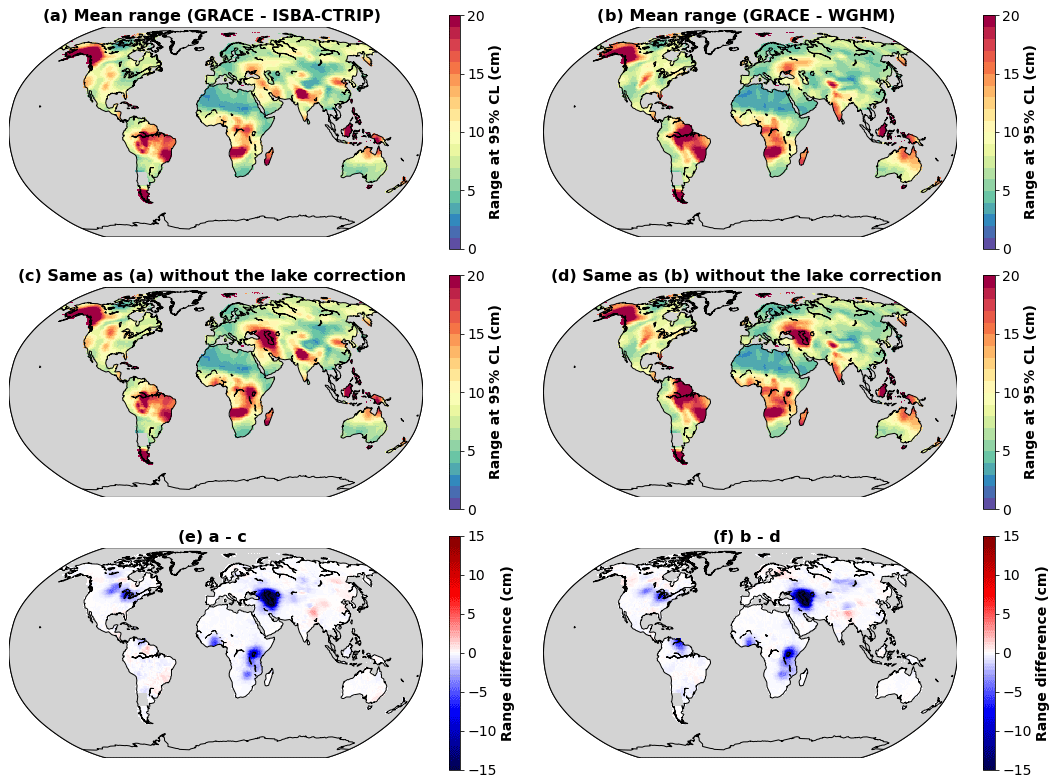
Figure A1(a) Range of residual TWS anomalies calculated with ISBA-CTRIP. (b) Range of residual TWS anomalies calculated with WGHM. (c) Range of residual TWS anomalies calculated with ISBA-CTRIP without including the lake correction. (d) Range of residual TWS anomalies calculated with WGHM without including the lake correction. (d) Difference between (a) and (c) due to the lake correction. (e) Difference between (b) and (d) due to the lake correction.
Residual TWS anomalies are calculated as the difference between the TWS anomalies estimated from GRACE and global hydrological models. The ensemble of residual TWS anomalies counts 18 solutions, pertaining to nine GRACE solutions (three mascon and six spherical harmonic solutions) and two global hydrological models (ISBA-CTRIP and WGHM). The range of average residual TWS anomalies shown in Fig. B1a depends on the systematic biases between the TWS estimates from GRACE and global hydrological models. These differences are significant if they exceed the dispersion among the 18 solutions, calculated as the difference between the 97.5 and 2.5 percentiles of the range of residual TWS anomalies (see Fig. B1b). The significance ratio of residual TWS anomalies (Fig. B1c) has been calculated to identify where the differences between GRACE solutions and hydrological models are significant, regardless of the solution or model considered. The dispersion of residual TWS solutions (Fig. B1b) is much larger than the dispersion of GRACE-based TWS solutions (Fig. 1b), showing that the differences between the two models may have a large impact on the residuals and their significance.
To explore a large variety of scenarios, we selected eight regions with large residuals (>10 cm) and high significance ratio (>2), including the Central Amazon Corridor (region A), the upper São Francisco River (region B), the Zambezi and Okavango rivers (region C), the Congo River (region D), the north of Australia (region E), the Ogallala aquifer in central United States (region F), the north of the Black Sea (region H) and the Northern Plains of India (region G). It may be noted that the significance ratio is not extremely high across the north of India because of the differences in the predictions of ISBA-CTRIP and WGHM. Region G was included to discuss the differences between models with respect to GRACE-based TWS anomalies. Glaciers and coastal regions have been excluded from the analyses (see Sect. 3.1).
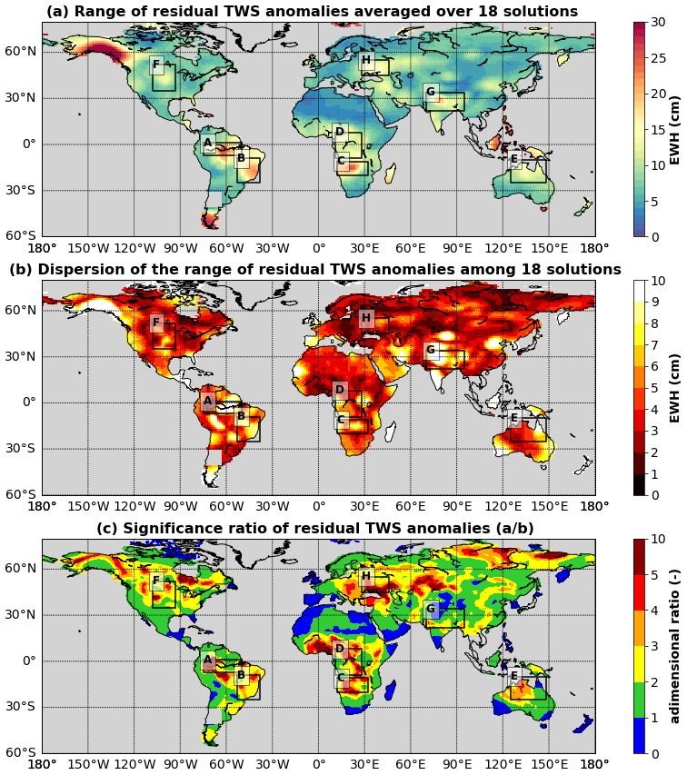
Figure B1(a) Average range of 18 residual TWS anomalies. (b) Dispersion of the range of residual TWS anomalies. The dispersion is calculated as the difference between the 97.5 and 2.5 percentiles of the range of 18 residual TWS anomalies. (c) Significance ratio of the averaged residual TWS anomalies calculated as the average range of residual TWS anomalies (a) divided by the dispersion of the range among the 18 solutions (b).
All code and data necessary to validate the research findings have been placed in a public repository at https://doi.org/10.5281/zenodo.7142392 (Pfeffer, 2022).
The supplement related to this article is available online at: https://doi.org/10.5194/hess-27-3743-2023-supplement.
All authors contributed to the conceptualisation of ideas presented in the manuscript. JP, AlB, BD and SM provided resources necessary to conduct the research findings. JP carried out the formal analysis. AC provided research supervision and funding acquisition. All authors contributed to the investigation of research findings. JP wrote the original draft. All authors contributed to the review and editing of the manuscript.
The contact author has declared that none of the authors has any competing interests.
Publisher’s note: Copernicus Publications remains neutral with regard to jurisdictional claims made in the text, published maps, institutional affiliations, or any other geographical representation in this paper. While Copernicus Publications makes every effort to include appropriate place names, the final responsibility lies with the authors.
This project has received funding from the European Research Council (ERC) under the European Union's Horizon 2020 Research and Innovation programme (GRACEFUL Synergy grant agreement no. 855677).
This research has been supported by the H2020 European Research Council (grant no. 855677).
This paper was edited by Micha Werner and reviewed by three anonymous referees.
Akvas: akvas/l3py: l3py v0.1.1 (v0.1.1), Zenodo [code], https://doi.org/10.5281/zenodo.1450900, 2018.
Alam, S., Gebremichael, M., Ban, Z., Scanlon, B. R., Senay, G., and Lettenmaier, D. P.: Post-Drought Groundwater Storage Recovery in California's Central Valley, Water Resour. Res., 57, e2021WR030352, https://doi.org/10.1029/2021WR030352, 2021.
Alsdorf, D., Beighley, E., Laraque, A., Lee, H., Tshimanga, R., O'Loughlin, F., Mahé, G., Dinga, B., Moukandi, G., and Spencer, R. G.: Opportunities for hydrologic research in the Congo Basin, Rev. Geophys., 54, 378–409, 2016.
Alsdorf, D. E., Rodríguez, E., and Lettenmaier, D. P.: Measuring surface water from space, Rev. Geophys., 45, 2, https://doi.org/10.1029/2006RG000197, 2007.
Anyah, R. O., Forootan, E., Awange, J. L., and Khaki, M.: Understanding linkages between global climate indices and terrestrial water storage changes over Africa using GRACE products, Sci. Total Environ., 635, 1405–1416, 2018.
Asoka, A., Gleeson, T., Wada, Y., and Mishra, V.: Relative contribution of monsoon precipitation and pumping to changes in groundwater storage in India, Nat. Geosci., 10, 109–117, 2017.
Becker, M., Papa, F., Frappart, F., Alsdorf, D., Calmant, S., da Silva, J. S., Prigent, C., and Seyler, F.: Satellite-based estimates of surface water dynamics in the Congo River Basin, Int. J. Appl. Earth Obs., 66, 196–209, 2018.
Bhanja, S. N., Mukherjee, A., Saha, D., Velicogna, I., and Famiglietti, J. S.: Validation of GRACE based groundwater storage anomaly using in-situ groundwater level measurements in India, J. Hydrol., 543, 729–738, 2016.
Bhanja, S. N., Mukherjee, A., Rodell, M., Wada, Y., Chattopadhyay, S., Velicogna, I., Pangaluru, K., and Famiglietti, J. S.: Groundwater rejuvenation in parts of India influenced by water-policy change implementation, Sci. Rep.-UK, 7, 1–7, 2017.
Birkett, C. M., Mertes, L. A. K., Dunne, T., Costa, M. H., and Jasinski, M. J.: Surface water dynamics in the Amazon Basin: Application of satellite radar altimetry, J. Geophys. Res.-Atmos., 107, 8059, https://doi.org/10.1029/2001JD000609, 2002.
Blazquez, A.: Satellite characterization of water mass exchange between ocean and continents at interannual to decadal timescales, Université Paul Sabatier – Toulouse III, English, NNT: 2020TOU30074, tel-03048246v2, 2020.
Bonnet, M. P., Barroux, G., Martinez, J. M., Seyler, F., Moreira-Turcq, P., Cochonneau, G., Melack, J. M., Boaventura, G., Maurice-Bourgoin, L., León, J. G., and Roux, E.: Floodplain hydrology in an Amazon floodplain lake (Lago Grande de Curuaí), J. Hydrol., 349, 18–30, 2008.
Brookfield, A. E., Hill, M. C., Rodell, M., Loomis, B. D., Stotler, R. L., Porter, M. E., and Bohling, G. C.: In situ and GRACE-based groundwater observations: Similarities, discrepancies, and evaluation in the High Plains aquifer in Kansas, Water Resour. Res., 54, 8034–8044, 2018.
Cáceres, D., Marzeion, B., Malles, J. H., Gutknecht, B. D., Müller Schmied, H., and Döll, P.: Assessing global water mass transfers from continents to oceans over the period 1948–2016, Hydrol. Earth Syst. Sci., 24, 4831–4851, https://doi.org/10.5194/hess-24-4831-2020, 2020.
Cai, W., Whetton, P. H., and Pittock, A. B.: Fluctuations of the relationship between ENSO and northeast Australian rainfall, Clim. Dynam., 17, 421–432, 2001.
Chen, J., Cazenave, A., Dahle, C., Llovel, W., Panet, I., Pfeffer, J., and Moreira, L.: Applications and challenges of GRACE and GRACE follow-on satellite gravimetry, Surv. Geophys., 1-41, 2022.
Chiew, F. H., Piechota, T. C., Dracup, J. A., and McMahon, T. A.: El Nino/Southern Oscillation and Australian rainfall, streamflow and drought: Links and potential for forecasting, J. Hydrol., 204, 138–149, 1998.
Condon, L. E., Kollet, S., Bierkens, M. F., Fogg, G. E., Maxwell, R. M., Hill, M. C., Fransen, H. J. H., Verhoef, A., Van Loon, A. F., Sulis, M., and Abesser, C.: Global groundwater modeling and monitoring: Opportunities and challenges, Water Resour. Res., 5, e2020WR029500, https://doi.org/10.1029/2020WR029500, 2021.
Crétaux, J. F., Abarca-del-Río, R., Berge-Nguyen, M., Arsen, A., Drolon, V., Clos, G., and Maisongrande, P.: Lake volume monitoring from space, Surv. Geophys., 37, 269–305, 2016.
Dahle, C., Flechtner, F., Murböck, M., Michalak, G., Neumayer, H., Abrykosov, O., Reinhold, A., and König, R.: GRACE Geopotential GSM Coefficients GFZ RL06, V. 6.0, GFZ Data Services, https://doi.org/10.5880/GFZ.GRACE_06_GSM, 2018.
Dangar, S., Asoka, A., and Mishra, V.: Causes and implications of groundwater depletion in India: A review, J. Hydrol., 596, 126103, 2021.
Da Silva, J. S., Seyler, F., Calmant, S., Rotunno Filho, O. C., Roux, E., Araújo, A. A. M., and Guyot, J. L.: Water level dynamics of Amazon wetlands at the watershed scale by satellite altimetry, Int. J. Remote Sens., 33, 3323–3353, 2012.
Decharme, B., Delire, C., Minvielle, M., Colin, J., Vergnes, J. P., Alias, A., Saint-Martin, D., Séférian, R., Sénési, S., and Voldoire, A.: Recent changes in the ISBA-CTRIP land surface system for use in the CNRM-CM6 climate model and in global off-line hydrological applications, J. Adv. Model. Earth Sy., 11, 1207–1252, 2019.
Dee, D. P., Uppala, S. M., Simmons, A. J., Berrisford, P., Poli, P., Kobayashi, S., Andrae, U., Balmaseda, M. A., Balsamo, G., Bauer, D. P., and Bechtold, P.: The ERA-Interim reanalysis: Configuration and performance of the data assimilation system, Quarterly Journal of the royal meteorological society, 137, 553–597, 2011.
De Jong, P., Tanajura, C. A. S., Sánchez, A. S., Dargaville, R., Kiperstok, A., and Torres, E. A: Hydroelectric production from Brazil's São Francisco River could cease due to climate change and inter-annual variability, Sci. Total Environ., 634, 1540–1553, 2018.
Deines, J. M., Schipanski, M. E., Golden, B., Zipper, S. C., Nozari, S., Rottler, C., Guerrero, B., and Sharda, V.: Transitions from irrigated to dryland agriculture in the Ogallala Aquifer: Land use suitability and regional economic impacts, Agr. Water Manage., 233, 106061, https://doi.org/10.1016/j.agwat.2020.106061, 2020.
Ditmar, P.: Conversion of time-varying Stokes coefficients into mass anomalies at the Earth's surface considering the Earth's oblateness, J. Geodesy, 92, 1401–1412, 2018.
Döll, P., Fritsche, M., Eicker, A., and Müller Schmied, H.: Seasonal water storage variations as impacted by water abstractions: comparing the output of a global hydrological model with GRACE and GPS observations, Surv. Geophys., 35, 1311–1331, 2014a.
Döll, P., Müller Schmied, H., Schuh, C., Portmann, F. T., and Eicker, A.: Global-scale assessment of groundwater depletion and related groundwater abstractions: Combining hydrological modeling with information from well observations and GRACE satellites, Water Resour. Res., 50, 5698–5720, 2014b.
Fan, Y., Li, H., and Miguez-Macho, G.: Global patterns of groundwater table depth, Science, 339, 940–943, 2013.
Fassoni‐Andrade, A. C., Fleischmann, A. S., Papa, F., Paiva, R. C. D. D., Wongchuig, S., Melack, J. M., Moreira, A. A., Paris, A., Ruhoff, A., Barbosa, C., and Maciel, D. A.: Amazon hydrology from space: scientific advances and future challenges, Rev. Geophys., 59, e2020RG000728, https://doi.org/10.1029/2020RG000728, 2021.
Felfelani, F., Wada, Y., Longuevergne, L., and Pokhrel, Y. N.: Natural and human-induced terrestrial water storage change: A global analysis using hydrological models and GRACE, J. Hydrol., 553, 105–118, 2017.
Fleischmann, A. S., Papa, F., Fassoni-Andrade, A., Melack, J. M., Wongchuig, S., Paiva, R. C. D., Hamilton, S. K., Fluet-Chouinard, E., Barbedo, R., Aires, F., and Al Bitar, A.: How much inundation occurs in the Amazon River basin?, Remote Sens. Environ., 278, 113099, https://doi.org/10.1016/j.rse.2022.113099, 2022.
Frappart, F., Papa, F., da Silva, J. S., Ramillien, G., Prigent, C., Seyler, F., and Calmant, S.: Surface freshwater storage and dynamics in the Amazon basin during the 2005 exceptional drought, Environ. Res. Lett., 7, 044010, https://doi.org/10.1088/1748-9326/7/4/044010, 2012.
Frappart, F., Papa, F., Güntner, A., Tomasella, J., Pfeffer, J., Ramillien, G., Emilio, T., Schietti, J., Seoane, L., da Silva Carvalho, J., and Moreira, D. M.: The spatio-temporal variability of groundwater storage in the Amazon River Basin, Adv. Water Resour., 124, 41–52, 2019.
Freitas, A. A., Drumond, A., Carvalho, V. S., Reboita, M. S., Silva, B. C., and Uvo, C. B.: Drought assessment in São Francisco river basin, Brazil: characterization through SPI and associated anomalous climate patterns, Atmosphere, 13, 41, https://doi.org/10.3390/atmos13010041, 2021.
Garzanti, E., Vermeesch, P., Vezzoli, G., Andò, S., Botti, E., Limonta, M., Dinis, P., Hahn, A., Baudet, D., De Grave, J., and Yaya, N. K.: Congo River sand and the equatorial quartz factory, Earth-Sci. Rev., 197, 102918, https://doi.org/10.1016/j.earscirev.2019.102918, 2019.
Girotto, M., De Lannoy, G. J. M., Reichle, R. H., Rodell, M., Draper, C., Bhanja, S. N., and Mukherjee, A.: Benefits and pitfalls of GRACE data assimilation: A case study of terrestrial water storage depletion in India, Geophys. Res. Lett., 44, 4107–4115, https://doi.org/10.1002/2017GL072994, 2017.
Gleeson, T., Smith, L., Moosdorf, N., Hartmann, J., Dürr, H. H., Manning, A. H., van Beek, L. P. H., and Jellinek, A. M.: Mapping permeability over the surface of the Earth, Geophys. Res. Lett., 38, L02401, https://doi.org/10.1029/2010GL045565, 2011.
Gleeson, T., Wagener, T., Döll, P., Zipper, S. C., West, C., Wada, Y., Taylor, R., Scanlon, B., Rosolem, R., Rahman, S., Oshinlaja, N., Maxwell, R., Lo, M.-H., Kim, H., Hill, M., Hartmann, A., Fogg, G., Famiglietti, J. S., Ducharne, A., de Graaf, I., Cuthbert, M., Condon, L., Bresciani, E., and Bierkens, M. F. P.: GMD perspective: The quest to improve the evaluation of groundwater representation in continental- to global-scale models, Geosci. Model Dev., 14, 7545–7571, https://doi.org/10.5194/gmd-14-7545-2021, 2021.
Goux, O., Pfeffer, J., Blazquez, A., Weaver, A. T., and Ablain, M.: Mass conserving filter based on diffusion for Gravity Recovery and Climate Experiment (GRACE) spherical harmonics solutions, Geophys. J. Int., 234, 56–72, https://doi.org/10.1093/gji/ggad016, 2023.
GRACE-FO: GRACEFO_L2_JPL_MONTHLY_060. Ver. 6. PO.DAAC, CA, USA, https://doi.org/10.5067/GFL20-MJ060, 2019a.
GRACE-FO: GRACEFO_L2_CSR_MONTHLY_0060. Ver. 6. PO.DAAC, CA, USA, https://doi.org/10.5067/GFL20-MC060, 2019b.
Haacker, E. M., Kendall, A. D., and Hyndman, D. W.: Water level declines in the High Plains Aquifer: Predevelopment to resource senescence, Groundwater, 54, 231–242, 2016.
Herbert, C. and Döll, P.: Global assessment of current and future groundwater stress with a focus on transboundary aquifers, Water Resour. Res., 55, 4760–4784, https://doi.org/10.1029/2018WR023321, 2019.
Houston, N. A., Gonzales‐Bradford, S. L., Flynn, A. T., Qi, S. L., Peterson, S. M., Stanton, J. S., Ryter, D. W., Sohl, T. L., and Senay, G. B.: Geodatabase Compilation of Hydrogeologic, Remote Sensing, and Water-Budget-Component Data for the High Plains Aquifer, 2011, US Geological Survey Data Series, 777, 12 pp., 2013.
Huffman, G. J., Stocker, E. F., Bolvin, D. T., Nelkin, E. J., and Tan, J.: GPM IMERG Final Precipitation L3 1 month 0.1 degree x 0.1 degree V06, Greenbelt, MD, Goddard Earth Sciences Data and Information Services Center (GES DISC), https://doi.org/10.5067/GPM/IMERG/3B-MONTH/06, 2019.
Hughes, D. A., Mantel, S., and Farinosi, F.: Assessing development and climate variability impacts on water resources in the Zambezi River basin: Initial model calibration, uncertainty issues and performance, J. Hydrol. Regional Studies, 32, 100765, https://doi.org/10.1016/j.ejrh.2020.100765, 2020.
Hugonnet, R., McNabb, R., Berthier, E., Menounos, B., Nuth, C., Girod, L., Farinotti, D., Huss, M., Dussaillant, I., Brun, F., and Kääb, A.: Accelerated global glacier mass loss in the early twenty-first century, Nature, 592, 726–731, https://doi.org/10.1038/s41586-021-03436-z, 2021.
Humphrey, V., Gudmundsson, L., and Seneviratne, S. I.: Assessing global water storage variability from GRACE: Trends, seasonal cycle, subseasonal anomalies and extremes, Surv. Geophys., 37, 357–395, 2016.
Junk, W. J.: The Central Amazon floodplain: Ecology of a pulsing system, Ecological Studies, Berlin, Germany, Springer, https://doi.org/10.1007/978-3-662-03416-3, 1997.
Kharlamov, M. and Kireeva, M.: Drought dynamics in the East European Plain for the period 1980–2018, in: E3S Web of Conferences (Vol. 163, p. 02004), EDP Sciences, https://doi.org/10.1051/e3sconf/202016302004, 2020.
Kitambo, B., Papa, F., Paris, A., Tshimanga, R. M., Calmant, S., Fleischmann, A. S., Frappart, F., Becker, M., Tourian, M. J., Prigent, C., and Andriambeloson, J.: A combined use of in situ and satellite-derived observations to characterize surface hydrology and its variability in the Congo River basin, Hydrol. Earth Syst. Sci., 26, 1857–1882, https://doi.org/10.5194/hess-26-1857-2022, 2022.
Kumar, S. V., Zaitchik, B. F., Peters-Lidard, C. D., Rodell, M., Reichle, R., Li, B., Jasinski, M., Mocko, D., Getirana, A., De Lannoy, G., and Cosh, M. H.: Assimilation of gridded GRACE terrestrial water storage estimates in the North American Land Data Assimilation System, J. Hydrometeorol., 17, 1951–1972, https://doi.org/10.1175/JHM-D-15-0157.1, 2016.
Labat, D., Ronchail, J., and Guyot, J. L.: Recent advances in wavelet analyses: Part 2–Amazon, Parana, Orinoco and Congo discharges time scale variability, J. Hydrol., 314, 289–311, 2005.
Lamontagne, S., Cook, P. G., O'Grady, A., and Eamus, D.: Groundwater use by vegetation in a tropical savanna riparian zone (Daly River, Australia), J. Hydrol., 310, 280–293, 2005.
Landerer, F. W., Flechtner, F. M., Save, H., Webb, F. H., Bandikova, T., Bertiger, W. I., Bettadpur, S. V., Byun, S. H., Dahle, C., Dobslaw, H., and Fahnestock, E.: Extending the global mass change data record: GRACE Follow-On instrument and science data performance, Geophys. Res. Lett., 47, e2020GL088306, https://doi.org/10.1029/2020GL088306, 2020.
Laraque, A., Moukandi N’kaya, G. D., Orange, D., Tshimanga, R., Tshitenge, J. M., Mahé, G., Nguimalet, C. R., Trigg, M. A., Yepez, S., and Gulemvuga, G.: Recent budget of hydroclimatology and hydrosedimentology of the congo river in central Africa, Water, 12, 2613, https://doi.org/10.3390/w12092613, 2020.
Lemoine, J.-M. and Bourgogne, S.: RL05 monthly and 10-day gravity field solutions from CNES/GRGS, GRACE/GRACE-FO Science Team Meeting 2020, online, 27–29 October 2020, GSTM2020-51, https://doi.org/10.5194/gstm2020-51, 2020.
Lesack, L. F.: Water balance and hydrologic characteristics of a rain forest catchment in the central Amazon basin, Water Resour. Res., 29, 759–773, 1993.
Lesack, L. F. and Melack, J. M.: Flooding hydrology and mixture dynamics of lake water derived from multiple sources in an Amazon floodplain lake, Water Resour. Res., 31, 329–345, 1995.
Li, B., Rodell, M., Kumar, S., Beaudoing, H. K., Getirana, A., Zaitchik, B. F., de Goncalves, L. G., Cossetin, C., Bhanja, S., Mukherjee, A., and Tian, S.: Global GRACE data assimilation for groundwater and drought monitoring: Advances and challenges, Water Resour. Res., 55, 7564–7586, https://doi.org/10.1029/2018WR024618, 2019.
Loomis, B. D., Luthcke, S. B., and Sabaka, T. J.: Regularization and error characterization of GRACE mascons, J. Geodesy, 93, 1381–1398, https://doi.org/10.1007/s00190-019-01252-y, 2019a.
Loomis, B. D., Rachlin, K. E., and Luthcke, S. B.: Improved Earth oblateness rate reveals increased ice sheet losses and mass-driven sea level rise, Geophys. Res. Lett., 46, 6910–6917, 2019b.
Lowman, L. E., Wei, T. M., and Barros, A. P.: Rainfall variability, wetland persistence, and water–carbon cycle coupling in the Upper Zambezi river basin in Southern Africa, Remote Sensing, 10, 692,https://doi.org/10.3390/rs10050692, 2018.
Lucas, M. C., Kublik, N., Rodrigues, D. B., Meira Neto, A. A., Almagro, A., Melo, D. D. C., Zipper, S. C., and Oliveira, P. T. S.: Significant baseflow reduction in the sao francisco river basin, Water, 13, 2, https://doi.org/10.3390/w13010002, 2020.
Luckey, R. and Becker, M.: Hydrogeology, water use, and simulation of flow in the High Plains Aquifer in north-western Oklahoma, southeastern Colorado, southwester Kansas, northeastern New Mexico, and northwestern Texas, Water-Resources Investigations Report 99-4104, Reston, Virginia: USGS, 1999.
Luckey, R. R., Gutentag, E. D., and Weeks, J. B.: Water-level and saturated thickness changes, predevelopment to 1980, in the High Plains Aquifer in parts of Colorado, Kansas, Nebraska, New Mexico, Oklahoma, South Dakota, Texas, and Wyoming, Hydrologic Investigations Atlas HA-652, Reston, Virginia: USGS, 1981.
Marzeion, B., Jarosch, A. H., and Hofer, M.: Past and future sea-level change from the surface mass balance of glaciers, The Cryosphere, 6, 1295–1322, https://doi.org/10.5194/tc-6-1295-2012, 2012.
Mayer-Gürr, T., Behzadpour, S., Ellmer, M., Kvas, A., Klinger, B., Strasser, S., and Zehentner, N.: ITSG-Grace2018 – Monthly, Daily and Static Gravity Field Solutions from GRACE, GFZ Data Services, https://doi.org/10.5880/ICGEM.2018.003, 2018.
Melack, J. M. and Coe, M. T.: Amazon floodplain hydrology and implications for aquatic conservation, Aquat. Conserv., 31, 1029–1040, 2021.
Meyer, U., Lasser, M., Jaeggi, A., Dahle, C., Flechtner, F., Kvas, A., Behzadpour, S., Mayer-Gürr, T., Lemoine, J., Koch, I., Flury, J., and Bourgogne, S.: International Combination Service for Time-variable Gravity Fields (COST-G) Monthly GRACE-FO Series, V. 01, GFZ Data Services, https://doi.org/10.5880/ICGEM.COST-G.002, 2020.
Mishra, V., Asoka, A., Vatta, K., and Lall, U.: Groundwater depletion and associated CO2 emissions in India, Earth's Future, 6, 1672–1681, 2018.
Müller Schmied, H., Cáceres, D., Eisner, S., Flörke, M., Herbert, C., Niemann, C., Peiris, T. A., Popat, E., Portmann, F. T., Reinecke, R., Schumacher, M., Shadkam, S., Telteu, C.-E., Trautmann, T., and Döll, P.: The global water resources and use model WaterGAP v2.2d: model description and evaluation, Geosci. Model Dev., 14, 1037–1079, https://doi.org/10.5194/gmd-14-1037-2021, 2021.
Ndehedehe, C. E. and Ferreira, V. G.: Assessing land water storage dynamics over South America, J. Hydrol., 580, 124339, https://doi.org/10.1016/j.jhydrol.2019.124339, 2020.
Ni, S., Chen, J., Wilson, C. R., Li, J., Hu, X., and Fu, R.: Global terrestrial water storage changes and connections to ENSO events, Surv. Geophys., 39, 1–22, 2018.
NOAA National Geophysical Data Center: ETOPO1 1 Arc-Minute Global Relief Model, NOAA National Centers for Environmental Information, https://repository.library.noaa.gov/view/noaa/1163 (last access: 18 October 2023), 2009.
O'Grady, A. P., Eamus, D., Cook, P. G., and Lamontagne, S.: Groundwater use by riparian vegetation in the wet–dry tropics of northern Australia, Aust. J. Bot., 54, 145–154, 2006.
Ojha, C., Shirzaei, M., Werth, S., Argus, D. F., and Farr, T. G.: Sustained groundwater loss in California's Central Valley exacerbated by intense drought periods, Water Resour. Res., 54, 4449–4460, 2018.
Papa, F., Crétaux, J. F., Grippa, M., Robert, E., Trigg, M., Tshimanga, R. M., Kitambo, B., Paris, A., Carr, A., Fleischmann, A. S., and de Fleury, M.: Water resources in Africa under global change: monitoring surface waters from space, Surv. Geophys., 44, 43–93, https://doi.org/10.1007/s10712-022-09700-9, 2022.
Paredes-Trejo, F., Barbosa, H. A., Giovannettone, J., Kumar, T. L., Thakur, M. K., Buriti, C. D. O., and Uzcátegui-Briceño, C.: Drought assessment in the São Francisco River Basin using satellite-based and ground-based indices, Remote Sensing, 13, 3921, https://doi.org/10.3390/rs13193921, 2021.
Paris, A., Calmant, S., Gosset, M., Fleischmann, A. S., Conchy, T. S. X., Garambois, P.-A., Bricquet, J.-P., Papa, F., Tshimanga, R. M., Guzanga, G. G., Siqueira, V. A., Tondo, B.-L., Paiva, R., da Silva, J. S., and Laraque, A.: Monitoring Hydrological Variables from Remote Sensing and Modeling in the Congo River Basin, in: Congo Basin Hydrology, Climate, and Biogeochemistry edited by: Tshimanga, R. M., N'kaya, G. D. M., and Alsdorf, D., https://doi.org/10.1002/9781119657002.ch18, 339–366, 2022.
Peltier, W. R., Argus, D. F., and Drummond, R.: Comment on the paper by Purcell et al. 2016 entitled An assessment of ICE-6G_C (VM5a) glacial isostatic adjustment model, J. Geophys. Res.-Sol. Ear., 122, 2016JB013844, https://doi.org/10.1002/2016JB013844, 2018.
Petheram, C., McMahon, T. A., and Peel, M. C.: Flow characteristics of rivers in northern Australia: implications for development, J. Hydrol., 357, 93–111, 2008.
Pfeffer, J.: supplementary-material-for-egusphere-2022-1032 (v0.0), Zenodo [data set], https://doi.org/10.5281/zenodo.7142392, 2022.
Pfeffer, J., Seyler, F., Bonnet, M.-P., Calmant, S., Frappart, F., Papa, F., Paiva, R. C. D., Satgé, F., and Silva, J. S. D.: Low-water maps of the groundwater table in the central Amazon by satellite altimetry, Geophys. Res. Lett., 41, 1981–1987, https://doi.org/10.1002/2013GL059134, 2014.
Pfeffer, J., Cazenave, A., and Barnoud, A.: Analysis of the interannual variability in satellite gravity solutions: detection of climate modes fingerprints in water mass displacements across continents and oceans, Clim. Dynam., 58, 1065–1084, 2022.
Prigent, C., Jimenez, C., and Bousquet, P.: Satellite-derived global surface water extent and dynamics over the last 25 years (GIEMS-2), J. Geophys. Res.-Atmos., 125, e2019JD030711, https://doi.org/10.1029/2019JD030711, 2020.
Quesada, C. A., Lloyd, J., Anderson, L. O., Fyllas, N. M., Schwarz, M., and Czimczik, C. I.: Soils of Amazonia with particular reference to the RAINFOR sites, Biogeosciences, 8, 1415–1440, https://doi.org/10.5194/bg-8-1415-2011, 2011.
RGI Consortium: Randolph Glacier Inventory – A Dataset of Global Glacier Outlines, Version 6. Boulder, Colorado USA, NSIDC: National Snow and Ice Data Center, https://doi.org/10.7265/4m1f-gd79, 2017.
Rateb, A., Scanlon, B. R., Pool, D. R., Sun, A., Zhang, Z., Chen, J., Clark, B., Faunt, C. C., Haugh, C. J., Hill, M., and Hobza, C.: Comparison of groundwater storage changes from GRACE satellites with monitoring and modeling of major US aquifers, Water Resour. Res., 5, e2020WR027556, https://doi.org/10.1029/2020WR027556, 2020.
Rodell, M., Houser, P. R., Jambor, U. E. A., Gottschalck, J., Mitchell, K., Meng, C. J., Arsenault, K., Cosgrove, B., Radakovich, J., Bosilovich, M., and Entin, J. K.: The global land data assimilation system, B. Am. Meteorol. Soc., 85, 381–394, 2004.
Rodell, M., Famiglietti, J. S., Wiese, D. N., Reager, J. T., Beaudoing, H. K., Landerer, F. W., and Lo, M. H.: Emerging trends in global freshwater availability, Nature, 557, 651–659, 2018.
Rouholahnejad, E., Abbaspour, K. C., Srinivasan, R., Bacu, V., and Lehmann, A.: Water resources of the Black Sea Basin at high spatial and temporal resolution, Water Resour. Res., 50, 5866–5885, 2014.
Rouholahnejad, E., Abbaspour, K. C., and Lehmann, A.: Water resources of the Black Sea catchment under future climate and land use change projections, Water, 9, 598, https://doi.org/10.3390/w9080598, 2017.
Save, H.: CSR GRACE and GRACE-FO RL06 Mascon Solutions v02, https://doi.org/10.15781/cgq9-nh24, 2020.
Save, H., Bettadpur, S., and Tapley, B. D.: High resolution CSR GRACE RL05 mascons, J. Geophys. Res.-Sol. Ea., 121, 7547–756, https://doi.org/10.1002/2016JB013007, 2016.
Scanlon, B. R., Longuevergne, L., and Long, D.: Ground referencing GRACE satellite estimates of groundwater storage changes in the California Central Valley, USA, Water Resour. Res., 48, W04520, https://doi.org/10.1029/2011WR011312, 2012a.
Scanlon, B. R., Faunt, C. C., Longuevergne, L., Reedy, R. C., Alley, W. M., McGuire, V. L., and McMahon, P. B.: Groundwater depletion and sustainability of irrigation in the US High Plains and Central Valley, P. Natl. Acad. Sci. USA, 109, 9320–9325, 2012b.
Scanlon, B. R., Zhang, Z., Save, H., Sun, A. Y., Müller Schmied, H., Van Beek, L. P., Wiese, D. N., Wada, Y., Long, D., Reedy, R. C., and Longuevergne, L.: Global models underestimate large decadal declining and rising water storage trends relative to GRACE satellite data, P. Natl. Acad. Sci. USA, 115, E1080–E1089, 2018.
Scanlon, B. R., Zhang, Z., Rateb, A., Sun, A., Wiese, D., Save, H., Beaudoing, H., Lo, M. H., Müller‐Schmied, H., Döll, P., and van Beek, R.: Tracking seasonal fluctuations in land water storage using global models and GRACE satellites, Geophys. Res. Lett., 46, 5254–5264, 2019.
Scanlon, B. R., Rateb, A., Anyamba, A., Kebede, S., MacDonald, A. M., Shamsudduha, M., Small, J., Sun, A., Taylor, R. G., and Xie, H.: Linkages between GRACE water storage, hydrologic extremes, and climate teleconnections in major African aquifers, Environ. Res. Lett., 17, 014046, https://doi.org/10.1088/1748-9326/ac3bfc, 2022.
Schneider, U., Becker, A., Finger, P., Meyer-Christoffer, A., Ziese, M., and Rudolf, B.: GPCC's new land surface precipitation climatology based on quality-controlled in situ data and its role in quantifying the global water cycle, Theor. Appl. Climatol., 115, 15–40, https://doi.org/10.1007/s00704-013-0860-x, 2014.
Schumann, G. J. P., Moller, D. K., Croneborg-Jones, L., and Andreadis, K. M.: Reviewing Applications of Remote Sensing Techniques to Hydrologic Research in Sub-Saharan Africa, with a Special Focus on the Congo Basin, Congo Basin Hydrology, Climate, and Biogeochemistry: A Foundation for the Future, 295–321, 2022.
Seyoum, W. M. and Milewski, A. M.: Monitoring and comparison of terrestrial water storage changes in the northern high plains using GRACE and in-situ based integrated hydrologic model estimates, Adv. Water Resour., 94, 31–44, 2016.
Sharmila, S. and Hendon, H. H.: Mechanisms of multiyear variations of Northern Australia wet-season rainfall, Sci. Rep., 10, 1–11, 2020.
Smith, I. N., Wilson, L., and Suppiah, R.: Characteristics of the northern Australian rainy season, J. Climate, 21, 4298–4311, 2008.
Smerdon, B. D., Gardner, W. P., Harrington, G. A., and Tickell, S. J.: Identifying the contribution of regional groundwater to the baseflow of a tropical river (Daly River, Australia), J. Hydrol., 464, 107–115, 2012.
Soltani, S. S., Ataie-Ashtiani, B., and Simmons, C. T.: Review of assimilating GRACE terrestrial water storage data into hydrological models: Advances, challenges and opportunities, Earth-Sci. Rev., 213, 103487, https://doi.org/10.1016/j.earscirev.2020.103487, 2021.
Steward, D. R. and Allen, A. J.: Peak groundwater depletion in the High Plains Aquifer, projections from 1930 to 2110, Agr. Water Manage., 170, 36–48, 2016.
Sun, Y., Riva, R., and Ditmar, P.: Optimizing estimates of annual variations and trends in geocenter motion and J2 from a combination of GRACE data and geophysical models, J. Geophys. Res.-Sol. Ea., 121, 8352–8370, 2016.
Sun, Z., Zhu, X., Pan, Y., and Zhang, J.: Assessing terrestrial water storage and flood potential using GRACE data in the Yangtze River basin, China. Remote Sensing, 9, 1011, https://doi.org/10.3390/rs9101011, 2017.
Tang, L., Li, J., Chen, J., Wang, S. Y., Wang, R., and Hu, X.: Seismic impact of large earthquakes on estimating global mean ocean mass change from GRACE, Remote Sensing, 12, 935, https://doi.org/10.3390/rs12060935, 2020.
Tapley, B. D., Bettadpur, S., Ries, J. C., Thompson, P. F., and Watkins, M. M.: GRACE measurements of mass variability in the Earth system, Science, 305, 503–505, 2004.
Thomas, B. F., Famiglietti, J. S., Landerer, F. W., Wiese, D. N., Molotch, N. P., and Argus, D. F.: GRACE groundwater drought index: Evaluation of California Central Valley groundwater drought, Remote Sens. Environ., 198, 384–392, 2017.
Tian, S., Renzullo, L. J., van Dijk, A. I. J. M., Tregoning, P., and Walker, J. P.: Global joint assimilation of GRACE and SMOS for improved estimation of root-zone soil moisture and vegetation response, Hydrol. Earth Syst. Sci., 23, 1067–1081, https://doi.org/10.5194/hess-23-1067-2019, 2019.
Tomasella, J., Hodnett, M. G., Cuartas, L. A., Nobre, A. D., Waterloo, M. J., and Oliveira, S. M.: The water balance of an Amazonian micro-catchment: The effect of interannual variability of rainfall on hydrological behaviour, Hydrol. Process., 22, 2133–2147, 2008.
Voldoire, A., Saint‐Martin, D., Sénési, S., Decharme, B., Alias, A., Chevallier, M., Colin, J., Guérémy, J. F., Michou, M., Moine, M. P., and Nabat, P.: Evaluation of CMIP6 DECK experiments with CNRM-CM6-1, J. Adv. Model. Earth Sy., 11, 2177–2213, https://doi.org/10.1029/2019MS001683, 2019.
Vörösmarty, C. J. and Moore, B.: Modeling basin-scale hydrology in support of physical climate and global biogeochemical studies: An example using the Zambezi River, Surv. Geophys., 12, 271–311, 1991.
Wada, Y., Wisser, D., and Bierkens, M. F. P.: Global modeling of withdrawal, allocation and consumptive use of surface water and groundwater resources, Earth Syst. Dynam., 5, 15–40, https://doi.org/10.5194/esd-5-15-2014, 2014.
Wahr, J., Molenaar, M., and Bryan, F.: Time variability of the Earth's gravity field: Hydrological and oceanic effects and their possible detection using GRACE, J. Geophys. Res.-Sol. Ea., 103, 30205–30229, 1998.
Ward, P. J., Beets, W., Bouwer, L. M., Aerts, J. C., and Renssen, H.: Sensitivity of river discharge to ENSO, Geophys. Res. Lett., 37, L12402, https://doi.org/10.1029/2010GL043215, 2010.
Weedon, G. P., Balsamo, G., Bellouin, N., Gomes, S., Best, M. J., and Viterbo, P.: The WFDEI meteorological forcing data set: WATCH Forcing Data methodology applied to ERA-Interim reanalysis data, Water Resour. Res., 50, 7505–7514, 2014.
Wiese, D. N., Yuan, D.-N., Boening, C., Landerer, F. W., and Watkins, M. M.: JPL GRACE and GRACE-FO Mascon Ocean, Ice, and Hydrology Equivalent Water Height JPL RL06 Version 02. Ver. 2. PO.DAAC, CA, USA, https://doi.org/10.5067/TEMSC-3MJ62, 2019.
Werth, S., Güntner, A., Petrovic, S., and Schmidt, R.: Integration of GRACE mass variations into a global hydrological model, Earth Planet. Sc. Lett., 277, 166–173, https://doi.org/10.1016/j.epsl.2008.10.021, 2009.
Xiang, L., Wang, H., Steffen, H., Wu, P., Jia, L., Jiang, L., and Shen, Q.: Groundwater storage changes in the Tibetan Plateau and areas revealed from GRACE satellite gravity data, Earth Planet. Sc. Lett., 449, 228–239, https://doi.org/10.1016/j.epsl.2016.06.002, 2016.
Xie, H., Longuevergne, L., Ringler, C., and Scanlon, B. R.: Integrating groundwater irrigation into hydrological simulation of India: Case of improving model representation of anthropogenic water use impact using GRACE, J. Hydrol. Regional Studies, 29, 100681, https://doi.org/10.1016/j.ejrh.2020.100681, 2020.
Xie, Z., Huete, A., Cleverly, J., Phinn, S., McDonald-Madden, E., Cao, Y., and Qin, F.: Multi-climate mode interactions drive hydrological and vegetation responses to hydroclimatic extremes in Australia, Remote Sens. Environ., 231, 111270, https://doi.org/10.1016/j.rse.2019.111270, 2019.
Yang, X., Tian, S., Feng, W., Ran, J., You, W., Jiang, Z., and Gong, X.: Spatio-temporal evaluation of water storage trends from hydrological models over Australia using GRACE mascon solutions, Remote Sensing, 12, 3578, https://doi.org/10.3390/rs12213578, 2020.
Yuan, D.-N.: GRACE Follow-On Level-2 Gravity Field Product User Handbook, JPL D-103922, https://podaac.jpl.nasa.gov/gravity/gracefo-documentation (last access: 20 October 2023), 2019.
Zaitchik, B. F., Rodell, M., and Reichle, R. H.: Assimilation of GRACE terrestrial water storage data into a land surface model: Results for the Mississippi River basin, J. Hydrometeorol., 9, 535–548, https://doi.org/10.1175/2007JHM951.1, 2008.
Zhuang, J., Dussin, R., Jüling, A., and Rasp, S.: JiaweiZhuang/xESMF: v0.3.0 Adding ESMF.LocStream capabilities (v0.3.0), Zenodo, https://doi.org/10.5281/zenodo.3700105, 2020.
- Abstract
- Introduction
- Methods
- Results
- Discussion
- Conclusions
- Appendix A: Comparison of TWS anomalies from GRACE and global hydrological models over large lakes
- Appendix B: Location of eight regions with significant residual TWS anomalies
- Code and data availability
- Author contributions
- Competing interests
- Disclaimer
- Acknowledgements
- Financial support
- Review statement
- References
- Supplement