What is the Priestley–Taylor wet-surface evaporation parameter? Testing four hypotheses

This study compares four different hypotheses regarding the nature of the Priestley–Taylor parameter α. They are as follows:

1. α is a universal constant.

2. The Bowen ratio ($H/LE$, where H is the sensible heat flux, and LE is the latent heat flux) for equilibrium (i.e., saturated air column near the surface) evaporation is a constant times the Bowen ratio at minimal advection (Andreas et al., 2013).

3. Minimal advection over a wet surface corresponds to a particular relative humidity value.

4. α is a constant fraction of the difference from the minimum value of 1 to the maximum value of α proposed by Priestley and Taylor (1972).

Formulas for α are developed for the last three hypotheses. Weather, radiation, and surface energy flux data from 171 FLUXNET eddy covariance stations were used. The condition $L{E}_{\mathrm{ref}}/L{E}_{\mathrm{p}}>$ 0.90 was taken as the criterion for nearly saturated conditions (where LE_ref is the reference, and LE_p is the apparent potential evaporation rate from the equation by Penman, 1948). Daily and monthly average data from the sites were obtained. All formulations for α include one model parameter which is optimized such that the root mean square error of the target variable was minimized. For each model, separate optimizations were done for predictions of the target variables α, wet-surface evaporation (α multiplied by equilibrium evaporation rate) and actual evaporation (the latter using a highly successful version of the complementary relationship of evaporation). Overall, the second and fourth hypotheses received the best support from the data.

1 Introduction

On a globe dominated by ocean surfaces, wet-surface evaporation has obvious global importance (e.g., Brutsaert, 2023, p. 142; Andreas, 2013; McMahon et al., 2013; Szilagyi et al., 2014; Yang and Roderick, 2019; Tu et al., 2022). But estimates of wet-surface evaporation can be valuable over land surfaces as well. For example, the Global Land Evaporation Amsterdam Model (GLEAM) evaporation product (Miralles et al., 2011; Martens et al., 2017) uses the Priestley–Taylor (1972) wet-surface evaporation equation as the starting point for land surface evaporation. While climatic influences on wet-surface evaporation rates can differ from those on transpiration (e.g., Schymanski and Or, 2015), in the GLEAM model, adjustments for water stress are made using a “multiplicative stress factor” (Martens et al., 2017). Many other models and data products use some form of the Penman (1948) or the related Penman–Monteith equation (Monteith, 1965; Allen et al., 1998; McMahon et al., 2013). The advection–aridity version (Brutsaert and Stricker, 1979) of Bouchet's (1963) complementary relationship (CR) between actual and apparent potential evaporation (Brutsaert, 2005, p. 136) makes use of both the Priestley–Taylor and the Penman equation to estimate actual land surface evaporation from non-saturated surfaces.

Both the Penman (1948) and the Priestley–Taylor (1972) equation are estimates of potential evaporation, the hypothetical evaporation rate that one would get from a land surface if the surface were saturated (Brutsaert; 2005, p. 136). The Penman equation consists of a radiative term and an advective term. Slatyer and McIlroy (1961, p. 3–73) noted that the advective term would be zero if the surface and the lower atmosphere were fully saturated (see further discussion in Sect. 2.1). Evaporation under this condition is known as equilibrium evaporation. The Priestley–Taylor equation multiplies the equilibrium evaporation rate by a factor α (where α>1) to account for the presence of some vapor pressure deficit, even under conditions of minimal advection – what Priestley and Taylor (1972) termed “the absence of advection”.

Some work regarding α for wet surfaces treated it as a global constant to be found through field experiments (e.g., Priestley and Taylor, 1972). Other work made use of mixed-layer models of the atmospheric boundary layer (ABL), linked to a surface layer model in order to assess the role of ABL development in the value of α (de Bruin, 1983; McNaughton, 1976; McNaughton and Spriggs, 1989; Lhomme, 1997a, b; Raupach, 2000). As a whole, this work suggests that ABL processes result in variability of the value of α. Since Priestley and Taylor (1972) found a single central value for α, such variability could cast doubt on the concept of a minimal-advection, wet-surface evaporation rate that can be reliably estimated. Eichinger et al. (1996) derived an explicit equation for α. Szilagyi et al. (2014) used global ocean data products to investigate α over the oceans of the world. They found a discernible relationship between α and temperature (see also Yang and Roderick, 2019). Han et al. (2021) began with the sigmoid generalized complementary equation developed by Han and Tian (2018) and modified it to apply to wet-surface evaporation.

The context of this work is the estimation of wet-surface evaporation, whether under actually wet conditions or the hypothetical evaporation rate if an unsaturated surface were actually saturated (Thornthwaite, 1948). Such hypothetical wet-surface evaporation estimates are commonly used, particularly in models based on the CR (e.g., Brutsaert and Stricker, 1979; Szilagyi and Joszsa, 2008; Crago et al., 2016; Han and Tian, 2018, 2020). In this context, it is not immediately apparent whether formulae derived for wet surfaces will also provide good results (for hypothetical wet-surface evaporation) from unsaturated surfaces. A different context is sometimes seen in the literature, in which α is essentially a moisture-availability factor (e.g., De Bruin, 1983). This latter use of α will not be further considered here.

The objective here is to gain a better conceptual understanding of α (cf., Crago and Qualls, 2013). Similar to the limitations applied by Priestley and Taylor (1972; cf. Andreas et al., 2013), only cases where both sensible and latent heat fluxes are positive will be considered.

Four hypotheses regarding α will be examined:

• Hypothesis 1. The ratio (α) between wet-surface evaporation under minimally advective conditions and under equilibrium conditions (i.e., a saturated atmospheric column near the wet surface) is a global constant.

• Hypothesis 2. There is a globally constant ratio (Andreas et al., 2013; Yang and Roderick, 2019) between (1) the Bowen ratio that occurs under minimal advection with a saturated surface and (2) the Bowen ratio that would occur under equilibrium evaporation conditions, and α can be derived using this constant ratio.

• Hypothesis 3. There is a globally constant relative humidity value that can be used to derive an estimate of α that corresponds to minimally advective conditions

• Hypothesis 4. The parameter α is a globally constant fraction of the gap between the minimum value of α and the maximum-allowable value of α proposed by Priestley and Taylor (1972).

All four hypotheses will be examined under actually saturated conditions, but they will also be evaluated under unsaturated conditions. Because there is no measured or reference value for the hypothetical wet-surface evaporation rate, instead the hypothetical rate will be included in a well-tested CR model for actual evaporation. That is, the CR model accuracy will be taken as an indirect measure of the method's ability to estimate the hypothetical wet-surface evaporation rate.

2 Theoretical background

2.1 Wet-surface evaporation equations

Latent heat flux LE (W m⁻²) is related to evaporation rate E (kg m⁻² s⁻¹) as LE =l_vE, where l_v is the latent heat of evaporation (J kg⁻¹). Penman's (1948) equation for apparent potential evaporation (LE_p) from a wet surface can be written as follows:

$$\begin{array}{}\text{(1)}& L{E}_{\mathrm{p}}={\displaystyle \frac{\mathrm{\Delta }}{\mathrm{\Delta }+\mathit{\gamma }}}\left(R_{\mathrm{n}}-G\right)+l_v{\displaystyle \frac{\mathit{\gamma }}{\mathrm{\Delta }+\mathit{\gamma }}}{E}_{\mathrm{A}},\end{array}$$

where $\mathrm{\Delta }=\mathrm{d}{e}^{*}/\mathrm{d}T$ (Pa K⁻¹) is evaluated at the air temperature T_a (K) at height z_T (m), e (Pa) is vapor pressure, and e^* (Pa) is saturated vapor pressure, where both e and e^* are calculated using the formulations given by Andreas et al. (2013) which are valid for temperatures both above and below freezing. The net radiation is R_n (W m⁻²); G (W m⁻²) is the ground heat flux; the latent heat of evaporation, l_v, is also calculated with a formulation given by Andreas (2013); $\mathit{\gamma }=c_{\mathrm{p}}p/(\mathrm{0.622}{l}_v$) (Pa K⁻¹) is the psychrometric constant; p (Pa) is atmospheric pressure; and c_p is the specific heat of air at constant pressure (J kg⁻¹ K⁻¹). The formulae adapted from Andreas et al. (2013) have been included in the Supplement. The drying power of the air E_A (kg m⁻² s⁻¹) is defined by

$$\begin{array}{}\text{(2)}& E_{\mathrm{A}}=f\left(u_{}\right)\left[e^{*}\left(T_{\mathrm{a}}\right)-e_{\mathrm{a}}\right],\end{array}$$

where e_a is the vapor pressure at height z_T and f(u) (s m⁻¹) is a function of wind speed. The wind function can be calculated (Brutsaert, 2015) using Monin–Obukhov similarity theory (MOS theory):

$$\begin{array}{}\text{(3)}& f\left(u\right)={\displaystyle \frac{\mathrm{0.622}{k}^{\mathrm{2}}u}{R_{\mathrm{d}}{T}_{\mathrm{a}}\ln \left[\left(z_T-d_{\mathrm{0}}\right)/z_{\mathrm{0}v}\right]\ln \left[\left(z_u-d_{\mathrm{0}}\right)/z_{\mathrm{0}}\right]}},\end{array}$$

where k=0.4 (dimensionless) is von Karman's constant; R_d (J kg⁻¹ K⁻¹) is the ideal gas constant of dry air; u (m s⁻¹) is wind speed measured at height z_T; d₀ (m) is the displacement height; and z₀ (m) and z_0v (m) are the roughness lengths for momentum and sensible heat, respectively. Equation (3) is based on MOS theory, the standard formulation of flux–gradient relationships in the lower atmosphere (Stull, 1988, p. 376; Brutsaert, 2005, p. 128), but Penman (1948) recommended the form f(u)=c₁(1+c₂u₂), where c₁ and c₂ are empirical constants, and u₂ (m s⁻¹) is wind speed at 2 m (m s⁻¹). This latter formulation (not used here) is preferred by some authors (e.g., Szilagyi et al., 2019) because information about the roughness of the surface (needed for z₀, z_0v and d₀) is not needed.

Note that other versions of LE_p are available, including one (e.g., Qualls and Crago, 2020; Crago and Qualls, 2021) which is based on the surface energy budget with mass and energy transport functions for the latent and sensible heat fluxes, respectively. While Eqs. (1)–(3) are based on the same principles, Penman's (1948) derivation involved his well-known approximation that Δ for a wet surface is approximately equal to the ratio of the difference in vapor pressure between the surface and measurement height to the difference in temperature between the same two levels, which allowed the simple two-term Eq. (1). Only Eq. (1) will be used for LE_p in this project.

As described by Brutsaert (2005, p. 129), air in the lowest layers blowing for a long distance over a wet surface would likely become increasingly humid. If it should approach saturation, the second term of (1) would go to zero, leaving the first term of (1) as an effective “lower limit” or “equilibrium value” for wet-surface evaporation (Slatyer and McIlroy, 1961, p. 3–73). This evaporation rate is often termed equilibrium evaporation (e.g., Brutsaert, 2005, p. 129). Here, this lower limit LE_e (W m⁻²) is calculated as

$$\begin{array}{}\text{(4)}& L{E}_{\mathrm{e}}={\displaystyle \frac{{\mathrm{\Delta }}_{T_{\mathrm{0}}}}{{\mathrm{\Delta }}_{T_{\mathrm{0}}}+\mathit{\gamma }}}\left(R_{\mathrm{n}}-G\right),\end{array}$$

where ${\mathrm{\Delta }}_{T_{\mathrm{0}}}$ is Δ evaluated at the wet-surface temperature T₀ (to be defined shortly). While Δ is commonly estimated at T_a, (e.g., Brutsaert, 2005, p. 126), Eq. (4) corresponds to the definition of equilibrium evaporation suggested by Andreas et al. (2014) and Qualls and Crago (2020). Namely, it is the lowest wet-surface evaporation rate possible for a given available energy value (R_n−G) with a surface temperature of T₀ (K). It is a minimum because lower evaporation rates would require the vapor pressure to exceed the saturation value (e.g., Philip, 1987; Andreas et al., 2013; Qualls and Crago, 2020). The fact that super-saturation cannot occur during evaporation explains why wet-surface evaporation is limited by Eq. (4) rather than simply by (R_n−G) (see Qualls and Crago, 2020). The Bowen ratio (Bo $=H/LE$; dimensionless) corresponding to Eq. (4) is Bo${}^{*}=$ ($R_{\mathrm{n}}-G-L{E}_{\mathrm{e}})/L{E}_{\mathrm{e}}$.

Priestley and Taylor (1972) introduced the parameter $\mathit{\alpha }=LE/L{E}_{\mathrm{e}}$(dimensionless) so that

$$\begin{array}{}\text{(5)}& L{E}_{\mathrm{PT}}=\mathit{\alpha }L{E}_{\mathrm{e}},\end{array}$$

where LE_PT (W m⁻²) estimates minimum-advection wet-surface latent heat flux. Because of some dry advection even over extensive saturated surfaces, they found α>1. Their data suggested a typical value of α≈ 1.26. Because LE_PT≥ LE_e and H≥ 0, the limits on α are (Priestley and Taylor, 1972)

$$\begin{array}{}\text{(6)}& \mathrm{1}\le \mathit{\alpha }\le \mathrm{1}+{\displaystyle \frac{\mathit{\gamma }}{{\mathrm{\Delta }}_{T_{\mathrm{0}}}}}.\end{array}$$

Hypothesis 1 suggests that Eq. (5), with α a global constant, defines minimal-advection wet-surface evaporation.

Andreas et al. (2013) examined thousands of measurements taken over extensive water and ice surfaces for which H>0 and LE >0 and suggested that Bo is related to Bo^* by

$$\begin{array}{}\text{(7)}& \mathrm{Bo}=a_{\mathrm{A}}{\mathrm{Bo}}^{*},\end{array}$$

where a_A (dimensionless) was found to be a global constant of about 0.4. This is equivalent to a Priestley–Taylor α of

$$\begin{array}{}\text{(8)}& {\mathit{\alpha }}_{\mathrm{A}}={\displaystyle \frac{{\mathrm{\Delta }}_{T_{\mathrm{0}}}+\mathit{\gamma }}{{\mathrm{\Delta }}_{T_{\mathrm{0}}}+a_{\mathrm{A}}\mathit{\gamma }}}.\end{array}$$

In Eq. (8), a_A is a constant, and Δ is a function of the skin temperature T₀ so that a discernible relationship between α and T₀ is implied by Eq. (8) (cf., Szilagyi et al., 2014). Hypothesis 2 suggests that Eq. (8) captures the foundational concept of α.

Yang and Roderick (2019) made a similar proposal to Eq. (7), resulting in a_A=0.24 based on global ocean data products. However, they noted that, in practice, LE and R_n cannot be known independently of each other over oceans, since increased LE reduces the ocean surface skin temperature, which reduces outgoing longwave radiant fluxes, thereby increasing R_n. Their value of a_A accounts for adjustments in the available energy resulting from this linkage. The present study assumes that R_n−G is known via measurements at each site.

Eichinger et al. (1996) had already proposed a dimensionless variable $C=\left[e^{*}\right(T_{\mathrm{a}})-e_{\mathrm{a}}]/\left[e^{*}\right(T_{\mathrm{0}})-e_{\mathrm{a}}$] for use in an explicit method (their Eq. 7) to estimate α for wet surfaces. Plans to include an additional hypothesis based on their Eq. (7) in this study were abandoned when it became apparent that their C (taken as a constant model parameter rather than calculated with the definition given in the previous sentence) is mathematically equivalent to (1−a_A). While we will refer to Eq. (8) as the Andreas et al. (2013) formula, we acknowledge the prescient contribution of Eichinger et al. (1996).

As an alternative to Eq. (8), if there is minimum advection over a wet surface, both Eqs. (1) and (5) should give the correct evaporation rate. By setting them equal to each other, one arrives at

$$\begin{array}{}\text{(9)}& {\mathit{\alpha }}_{\mathrm{RH}}=\mathrm{1}+\left({\displaystyle \frac{\mathit{\gamma }}{{\mathrm{\Delta }}_{T_{\mathrm{0}}}}}\right){\displaystyle \frac{l_{v}f\left(u\right)e^{*}\left(T_{\mathrm{0}}\right)\left(\mathrm{1}-\mathrm{RH}\right)}{R_{\mathrm{n}}-G}}.\end{array}$$

where RH (dimensionless) is the relative humidity of the air, and α_RH is dimensionless. The values of l_v, ${\mathrm{\Delta }}_{T_{\mathrm{0}}}$, and e^* could all be evaluated at the wet-surface skin temperature T₀. Equation (9) gives the correct value of α within the accuracy of Penman's (1948) assumption regarding Δ, provided RH is the measured relative humidity. However Eq. (9) is proposed here as a parameterization of α for both actually and hypothetically saturated surfaces, where RH is the model parameter representing the relative humidity under saturated surface and minimal advection conditions. Small values of (R_n−G) could result in unreasonably large values of α. Therefore, the limits given by Eq. (6) are applied to estimates of α_RH. That is, if ${\mathit{\alpha }}_{\mathrm{RH}}>\mathrm{1}+\mathit{\gamma }/\mathrm{\Delta }$, it is set to $\mathrm{1}+\mathit{\gamma }/\mathrm{\Delta }$, and if α_RH<1, then it is set to 1.

The limits on α given by Eq. (6) suggest that perhaps α takes a constant intermediate position in between the limits. Thus, the parameter m (dimensionless) is

$$\begin{array}{}\text{(10)}& m={\displaystyle \frac{\mathit{\alpha }-\mathrm{1}}{\left(\mathrm{1}+\frac{\mathit{\gamma }}{{\mathrm{\Delta }}_{T_{\mathrm{0}}}}\right)-\mathrm{1}}}\end{array}$$

or

$$\begin{array}{}\text{(11)}& \mathit{\alpha }=\mathrm{1}+m{\displaystyle \frac{\mathit{\gamma }}{{\mathrm{\Delta }}_{T_{\mathrm{0}}}}}.\end{array}$$

Hypothesis 4 suggests that Eq. (11) is the best explanation of α.

Szilagyi and Jozsa (2008; see also Szilagyi and Schepers, 2014; Szilagyi et al., 2017) suggested T₀ could be found by setting two expressions for the Bowen ratio (here, given by $H/L{E}_{\mathrm{p}}$) equal to each other:

$$\begin{array}{}\text{(12)}& {\displaystyle \frac{R_{\mathrm{n}}-G-L{E}_{\mathrm{p}}}{L{E}_{\mathrm{p}}}}=\mathit{\gamma }{\displaystyle \frac{T_{\mathrm{0}}-T_{\mathrm{a}}}{e^{*}\left(T_{\mathrm{0}}\right)-e_{\mathrm{a}}}},\end{array}$$

where the equation used for e^*(T₀) (from Andreas et al., 2014) is given in the Supplement. The wet-surface temperature in Eq. (12) is T₀, which can be easily found from Eq. (12) with a numerical root finder. Equation (12), thus solved, provides the wet-surface temperature T₀ from data taken from either saturated or unsaturated surfaces (Szilagyi and Schepers, 2014).

2.2 The complementary relationship (CR) of evaporation

In the complementary relationship (CR) between actual and potential evaporation (Bouchet, 1963), regional evaporation from a saturated surface, the apparent-potential evaporation rate, and the actual evaporation rate are all identical (Brutsaert, 2015, p. 136). According to the advection–aridity approach (Brutsaert and Stricker, 1979), apparent potential evaporation corresponds to Penman's equation (Eq. 1) or to the evaporation from a small wet patch, and the wet regional surface rate corresponds to the Priestley –Taylor equation (1972), shown in Eq. (5). As the surface dries, less water is available to evaporate, so actual evaporation decreases. This results in a drier and warmer lower atmosphere, which increases apparent potential (wet patch) evaporation. Conversely, if the lower atmosphere becomes dry and warm (in the absence of significant dry advection), this implies that regional evaporation rates are low. Thus, evaporation and apparent potential evaporation change in opposite directions – they complement each other. An estimate of the Priestley–Taylor α is an integral part of most CR models, and the performance of CR models making use of the four different hypotheses regarding α can serve as a further test of the hypotheses. Note that Han et al. (2021) took a different approach, by adapting the CR model of Han and Tian (2018) to estimate evaporation from wet surfaces; this results in a non-linear dependence of wet-surface evaporation on equilibrium evaporation.

As formulated by Brutsaert (2015, p. 136), the CR can be formulated in terms of x= $L{E}_{\mathrm{w}}/L{E}_{\mathrm{p}}$ and $y=LE/L{E}_{\mathrm{p}}$, where LE_w is given by Eq. (5) and LE_p by Eqs. (1)–(3). Both x and y are dimensionless. Values of α to be used in Eq. (5) will be discussed in Sect. 3. Brutsaert (2015) used physical reasoning to suggest that at x= 0, the boundary conditions are y= 0 and d$y/\mathrm{d}x=\mathrm{0}$, while at x= 1, they are y= 1 and d$y/\mathrm{d}x=$ 1. Crago et al. (2016), however, noted that y can approach zero when there is no water available to evaporate, but x cannot approach zero unless LE_w goes to zero. The smallest x can get is

$$\begin{array}{}\text{(13)}& x_{\min }={\displaystyle \frac{L{E}_{\mathrm{w}}}{L{E}_{{\mathrm{p}}_{\max }}}},\end{array}$$

where $L{E}_{{\mathrm{p}}_{\max }}$ (W m⁻²) is given by

$$\begin{array}{}\text{(14)}& L{E}_{{\mathrm{p}}_{\max }}={\displaystyle \frac{{\mathrm{\Delta }}_{\mathrm{d}}}{{\mathrm{\Delta }}_{\mathrm{d}}+\mathit{\gamma }}}\left(R_{\mathrm{n}}-G\right)+l_v{\displaystyle \frac{\mathit{\gamma }}{{\mathrm{\Delta }}_{\mathrm{d}}+\mathit{\gamma }}}f\left(u\right)e^{*}\left(T_{\mathrm{d}}\right).\end{array}$$

In Eq. (15), the subscript “d” means the variable is evaluated at T_d, the “dry air temperature”. A straight line with slope d$e/\mathrm{d}{T}_{\mathrm{g}}=-\mathit{\gamma }$ (where T_g is a generic temperature variable) represents an isenthalp (line of constant available energy) through (T_a, e_a) on a graph of temperature (x axis) versus vapor pressure (e on the y axis). The temperature at which this isenthalp reaches e= 0 is T_d (Szilagyi et al., 2017; Crago and Qualls, 2021). That is,

$$\begin{array}{}\text{(15)}& T_{\mathrm{d}}=T_{\mathrm{a}}+{\displaystyle \frac{e_{\mathrm{a}}}{\mathit{\gamma }}}.\end{array}$$

Crago et al. (2016) suggested x could be “rescaled” through the following transform:

$$\begin{array}{}\text{(16)}& X={\displaystyle \frac{x-x_{\min }}{\mathrm{1}-x_{\min }}}.\end{array}$$

A simple formulation suggested by Crago et al. (2016) is

$$\begin{array}{}\text{(17)}& y=X.\end{array}$$

Crago et al. (2022) considered data from seven FLUXNET sites in Australia as well as global, gridded ERA5 data (Hersbach, 2020) produced by ECMWF (European Centre for Medium-Range Weather Forecasts; https://www.ecmwf.int/, last access: 23 August 2023). With the FLUXNET data, Eq. (17) consistently performed best at predicting reference (eddy covariance) latent heat fluxes. Since FLUXNET data are used here as well, Eq. (17) will be the assumed CR formula for this study. From Eq. (17), latent heat flux estimates can be found with LE_est=X(LE_p).

Equations (1)–(5) and CR methods are generally considered applicable at timescales ranging from daily to monthly, with monthly being most common (McMahon et al., 2013). Equations (1)–(5) require homogeneous surfaces corresponding to the spatial extent of the flux footprint (e.g., Schuepp, 1990), typically corresponding to several hundred meters, while CR formulations are best suited for homogeneous conditions at the “regional” scale (Brutsaert, 2005, p. 136) of perhaps tens of kilometers.

3 Methodology

3.1 Data sources and processing

Monthly- and daily-average data pre-processed by FLUXNET were downloaded as CSV files from the fluxnet.org website for 171 eddy covariance stations (listed in Table S1 in the Supplement). At least minimally adequate fetches are assumed at all sites included in FLUXNET. Measurement heights, latitudes, longitudes, IGBP (International Geosphere-Biosphere Programme) land classes (https://www.igbp.net, last access: 23 August 2023), and canopy heights were provided for these sites by Wang et al. (2020; see their supporting information). Wang et al. (2020) assumed z₀=0.123h_c, d₀=0.67h_c, and z_0v=0.1z₀, where h_c (m) is the reported canopy height. These values were all adopted herein. Separate wind speed, temperature, and humidity measurement heights were not included by Wang et al. (2020), so it is assumed here that they are all measured at the single given height. Net radiation, ground heat flux, sensible and latent heat fluxes, air pressure, air temperature, vapor pressure deficit, and wind speed were included in the FLUXNET downloads. All variables employed some gap filling using the MDS (marginal distribution sampling; Reichstein, 2005) method as described by Pastorello et al. (2020). Data flagging and quality assurance and control for all the variables also followed the procedures outlined by Pastorello et al. (2020). The data and the software used in this project are available through Zenodo and GitHub (see Crago et al., 2023a, b).

Following the procedures outlined by Pastorello et al. (2020), the half-hourly or hourly energy fluxes are also gap-filled using the MDS (Reichstein, 2005) method, and these are used by FLUXNET to derive the daily or monthly reference values used here. The FLUXNET dataset includes the variables “H_CORR” and “LE_CORR”, which indicate corrected values, that is, values that correspond to energy budget closure. However, the corresponding uncorrected variables (“LE_F_MDS” and “H_F_MDS”) are available for more sites and times. These latter surface fluxes were used for this study for the reference values LE_ref and H_ref, respectively. Issues regarding energy budget closure with eddy covariance fluxes are complicated, as discussed by Mauder et al. (2020). In this study, the downloaded values of sensible heat flux are taken to be the final reference values H_ref, while downloaded latent heat flux values are adjusted so that monthly (daily) energy budget closure is obtained: $L{E}_{\mathrm{ref}}=(R_{\mathrm{n}}-G)-H_{\mathrm{ref}}$. This was the procedure recommended by Wang et al. (2020; see also Tu et al., 2022, 2023).

Months (or days) with eddy covariance values of H and LE less than zero or $R_{\mathrm{n}}-G<\mathrm{0}$ were screened out of the dataset; this eliminates periods of strong dry advection that result in negative H_ref. The ground heat flux G was not measured at all for some of the sites, and missing values of G also occurred. When measurements of G were not available, a value of zero was assumed. Over a 24 h period, G “is often near zero” (Stull, 1988), so this assumption is not unreasonable. Over the daily to monthly timescales at which Eqs. (1) and (5) are commonly used (McMahon, 2014), the assumption likely improves as the averaging time increases.

The CR has been used at timescales from hours to years (Brutsaert, 2023, p. 147), but the CR, the Penman equation (Eq. 1), and the Priestley–Taylor equation (Eq. 5) most typically use daily- to monthly-average values (McMahon, 2013). It is true that use of time averages of variables as inputs to non-linear equations can lead to “significant errors” (Slatyer and McIlroy, 1961, p. 3–58). However, CR and the Priestley–Taylor wet-surface equation both assume that the land surface conditions and the temperature and humidity in the lower atmosphere are well adjusted to each other (Brutsaert, 2023, p. 147). The diurnal cycle makes this adjustment unlikely over periods less than 24 h (McMahon, 2013). Therefore, the approach here is to use daily-average (monthly-average) input values to produce daily (monthly) energy fluxes (e.g., Penman, 1948; McMahon, 2013; Brutsaert, 2023). That is, daily to monthly timescales are suited to these equations, as spatial scales corresponding to small watersheds are suited to saturation-excess runoff (e.g., Chow et al., 1988).

With this dataset, the monthly (daily) mean of reference latent heat flux is 61 W m⁻² (62 W m⁻²), the median is 58 W m⁻² (56 W m⁻²), and the standard deviation is 41 W m⁻² (48 W m⁻²). Thus, the central tendencies for monthly and daily values are similar, but the daily values have more spread about the mean.

The decisions described above regarding data inclusion, screening, and correction reflect a desire to obtain a broad range of climates, land covers, and seasons, so as to test the four hypotheses under as wide a range of conditions as possible. While these decisions do entail some risk of including lower quality data, we think they are defendable as outlined above. However, much of the analysis was repeated after removing data for which the FLUXNET quality control index (which ranges from 0 for very poor to 1 for excellent) was less than 0.9, with little difference in numerical results and no difference in qualitative results (such as which methods performed better than other methods) compared to the results without filtering for data quality.

A total of 11 different IGBP land surface classes (e.g., Loveland et al., 1999) are in the original data. They include Wooded Savanna (WSA), Grassland (GRA), Evergreen Broadleaf Forest (EBF), Cropland (CRO), Evergreen Needleleaf Forest (ENF), Savanna (SAV), Deciduous Broadleaf Forest (DBF), Closed Shrubland (CSH), Mixed Forest (MF), Open Shrubland (OSH), and Permanent Wetland (WET). Classes for each site were provided by Wang et al. (2020).

3.2 Estimates of wet-surface α

Determination of wet-surface values of α requires determination of data representing saturated surface conditions. Saturated or nearly saturated land surface conditions were assumed when LE_ref>T(LE_p), where T (dimensionless) is a threshold value which had to be determined. A value of T was sought such that the linear regression between LE_ref and LE_p (for data for which the condition above is met) falls nearly on the 1 : 1 line, and at the same time root mean square (rms) errors between LE_ref and LE_p are very small. After filtering for wet-surface conditions, α_ref was calculated as $LE/L{E}_{\mathrm{e}}$.

Trial values of the parameters α_c, a_A, RH, and m, where α_c is a constant (global) value of α, were selected randomly from a range of reasonable values (that is, α ranged from 1 to 1.6, and a_A, RH, and m all varied from 0 to 1). These values were used at all sites and times, satisfying the wet-surface condition. A total of 3000 values drawn randomly from these ranges were evaluated to determine the optimal parameter values. These optimal parameter values were used to estimate different versions of α_est, namely α_c and a_A from Eq. (8), α_RH from Eq. (9), and α_m from Eq. (11). These α_est values were compared to α_ref= $L{E}_{\mathrm{ref}}/L{E}_{\mathrm{e}}$. The trial parameter values that minimized the root mean square difference (RMSD) between α_est and α_ref were taken to the be tuned parameter values; the values of α_est will be called the best-fit values.

3.3 Estimates of wet-surface evaporation

Randomly selected parameter values were chosen 3000 times (over the same range as in Sect. 3.2) to estimate α_c, α_A, α_RH, and α_m for use in Eq. (5) to estimate LE_est=α_estLE_e, where α_est is estimated from the parameter values using Eqs. (8), (9), and (11). This was done for all wet-surface measurements. Tuned parameter values were those giving minimum RMSD between the resulting LE_est and LE_ref, and the resulting LE_est values are considered best-fit values. The same tuned parameter values were used for all stations and all times. Note that the tuned parameter values found in this analysis may differ from those found in Sect. 3.2.

3.4 Complementary relationship for actual evaporation

Next, actual evaporation was estimated with the CR using all available data. That is, the analysis was not limited to only wet-surface data. Specifically, 3000 new samples of the parameter values were chosen from the same range as above. Those parameter values were substituted into Eqs. (8), (9), or (11) and were used to calculate estimates of α. Those values in turn were used in Eqs. (1)–(5) along with Eqs. (14)–(16) in Eq. (17) and finally in $L{E}_{\mathrm{est}}=y\times L{E}_{\mathrm{p}}$. The RMSD between LE_est and LE_ref was found for each of the four methods of estimating LE_PT. The tuned parameter values were those minimizing the RMSD, and the corresponding LE_ref values are the best-fit values.

4 Results

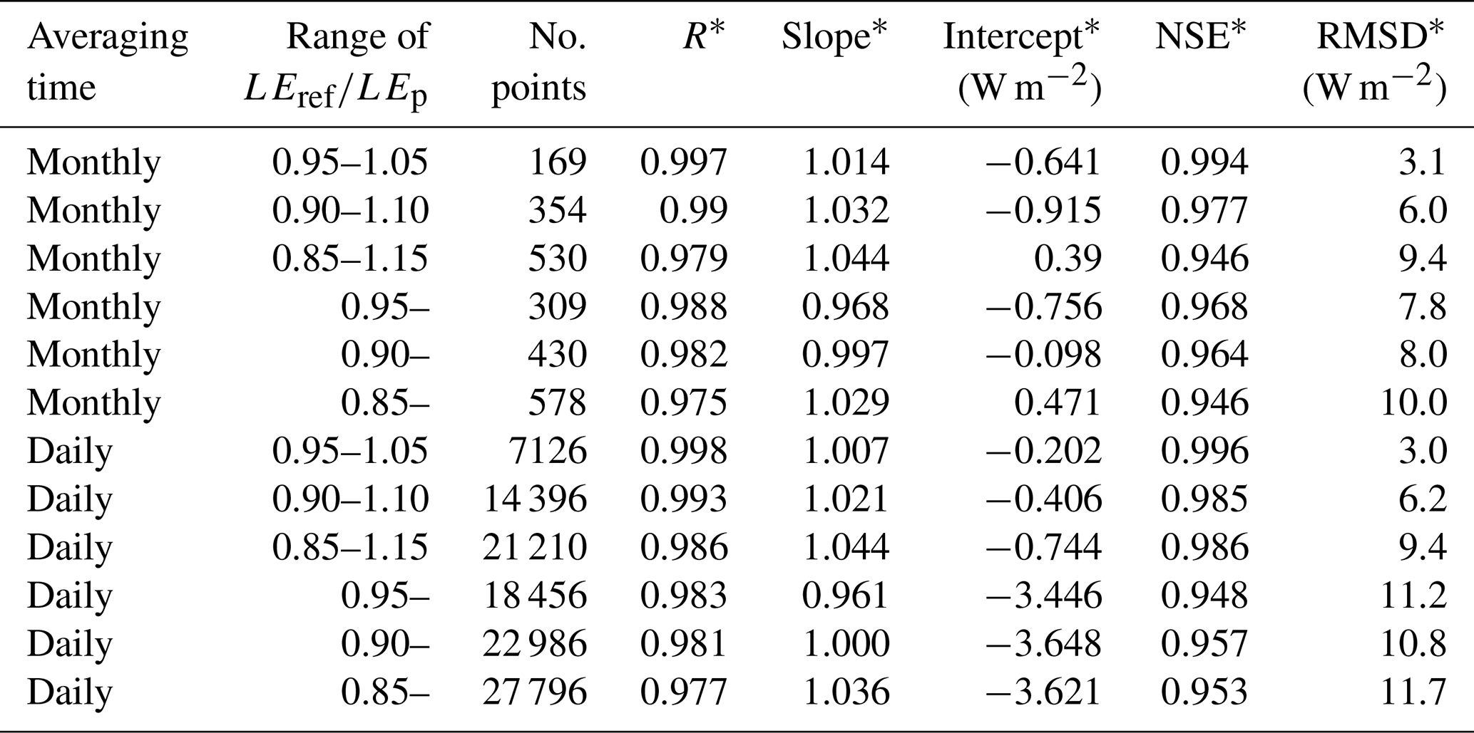
For monthly averaging times, the wet-surface threshold was established to be T=0.90, which resulted in a regression equation with slope of about 1 and intercept very near 0, while rms errors were small (Fig. 1d). The process by which this value of T was established is described using Fig. 1, and the corresponding statistics for both monthly and daily data are found in Table 1. The second row of text in each panel identifies the range of $L{E}_{\mathrm{ref}}/L{E}_{\mathrm{p}}$ values incorporated into the graph. If the lower limit of accepted values was T, then in the left column (Fig. 1a, c, e) an upper limit of 2−T was imposed. In the right column (Fig. 1b, d, f) no upper limit was imposed (as indicated by an upper limit denoted “−”). There seems to be no compelling reason to impose an upper limit on wet-surface $L{E}_{\mathrm{ref}}/L{E}_{\mathrm{p}}$, even though the upper limit improved many of the statistics (i.e., comparing Fig. 1a to b, c to d, and e to f). Figure 1b has a slope somewhat below 1a, and Fig. 1f has a large RMSD. Figure 1d, where all points with $L{E}_{\mathrm{ref}}/L{E}_{\mathrm{p}}>\mathrm{0.90}$ were included, was taken as a reasonable compromise. As shown in Fig. 1d, wet-surface evaporation defined in this way occurred in 430 months and from 50 of the sites. The sites included IGBP classes CRO, ENF, GRA, DBF, WET, OSH, and EBF. For daily averaging times, a similar process was followed (statistics included in Table 1). Wet-surface evaporation (defined again by T=0.90) occurred on 22 998 d, involving 158 of the 171 stations, and included IGBP classes WSA, GRA, EBF, CRO, ENF, SAV, DBF, CSH, OSH, WET, and MF. Figure 2 shows the location of sites having at least 1 month of wet-surface measurements (top panel) and those having none (bottom panel).

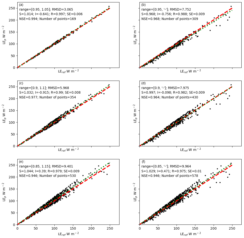
Figure 1 Comparison of reference values (LE_ref) to estimates of LE_est from Eq. (1) for various threshold (T) values to define wet-surface conditions for monthly evaporation. In each plot, only data from a given range of $L{E}_{\mathrm{ref}}/L{E}_{\mathrm{p}}$ are plotted and included in the statistics included in the upper-left corner of each plot. Panels (a, c, e) apply both upper and lower limits on $L{E}_{\mathrm{ref}}/L{E}_{\mathrm{p}}$, while panels (b, d, f) only apply a lower limit. Panel (d) was taken as the best compromise, as it has many desired features, including a relatively large number of points, regression slopes near 1, intercepts near zero, and low RMSDs. A total of 430 months of wet-surface evaporation were identified. RMSD is the root mean square difference, R is the correlation coefficient, NSE is the Nash–Sutcliffe efficiency (Nash and Sutcliffe, 1970), and S and I are the slope and intercept in the linear regression equation. The “range” in the second line of text in each plot indicates the range of $L{E}_{\mathrm{p}}/L{E}_{\mathrm{ref}}$ values included in the analysis, with the first number in brackets indicating the lower and the second number the higher limit of the range; the notation “−” indicates no upper limit. The dashed red line is 1 : 1, and the dotted green line represents the linear regression.

Table 1 Results of regression between LE_p and LE_ref for various ranges of $L{E}_{\mathrm{ref}}/L{E}_{\mathrm{p}}$.

^* R: correlation coefficient. Slope and intercept: S and I in $L{E}_{\mathrm{p}}=S\times L{E}_{\mathrm{ref}}+I$. NSE: Nash–Sutcliffe (1970) efficiency. RMSD: root mean square difference. Range values ending with “–” indicate no upper limit to the range.

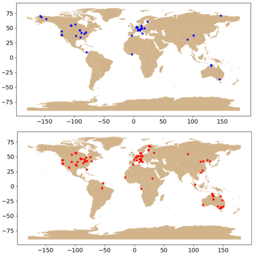
Figure 2 Global distribution of sites with some monthly measurements classified as wet-surface evaporation (top panel) and those with no wet-surface values (bottom panel). For daily average data, many more sites had some days of wet-surface evaporation, so for daily averaging, the top panel would have more data points and the bottom panel fewer. The background map is the “naturalearth_lowres” basemap provided by geopandas (https://geopandas.org, last access: 23 August 2023).

As described in Sect. 3.2, using only wet-surface measurements, tuned values of α_c, a_A, RH, and m were found that minimized RMSD between reference and estimated values of α. Different tuned values of these parameters were also found for use in estimating wet-surface evaporation using the Priestley–Taylor equation (Eq. 5). Results for estimating α under wet-surface conditions are found in Fig. 3a, and results for estimating wet-surface evaporation itself are shown in Fig. 3b; both sets of results are also provided in Table 2. Finally, still-different tuned values of α_c, a_A, RH, and m were those which produced the minimum values of RMSD between LE_est and LE_ref using the CR formulation in Eq. (17). That is, LE_est is found by taking y found with Eq. (17), where LE_w is given by Eq. (5), LE_p by Eqs. (1)–(3), and y by Eqs. (13)–(17). This y was multiplied by LE_p from Eq. (1) to get LE_est. The tuned parameters that result when the goal is to obtain the best fit between α_est and α_ref are different than those when the goal is to obtain the best fit between wet-surface LE_PT and LE_ref, and in turn these are different than when the goal is to obtain the best fit between LE_est and LE_ref using Eq. (17). Reasons and implications for these differences will be discussed in Sect. 5.

Figure 3 Results for monthly estimates of (a) wet-surface α and of (b) wet-surface LE. Parameter values and statistics are included at the top of each graph. RMSD is the root mean square difference, R is the correlation coefficient, NSE is the Nash–Sutcliffe (1970) efficiency, and S and I are the coefficients in the linear regression equation.

Table 2 Summary of results for monthly data (430 wet-surface months; 9980 months in total).

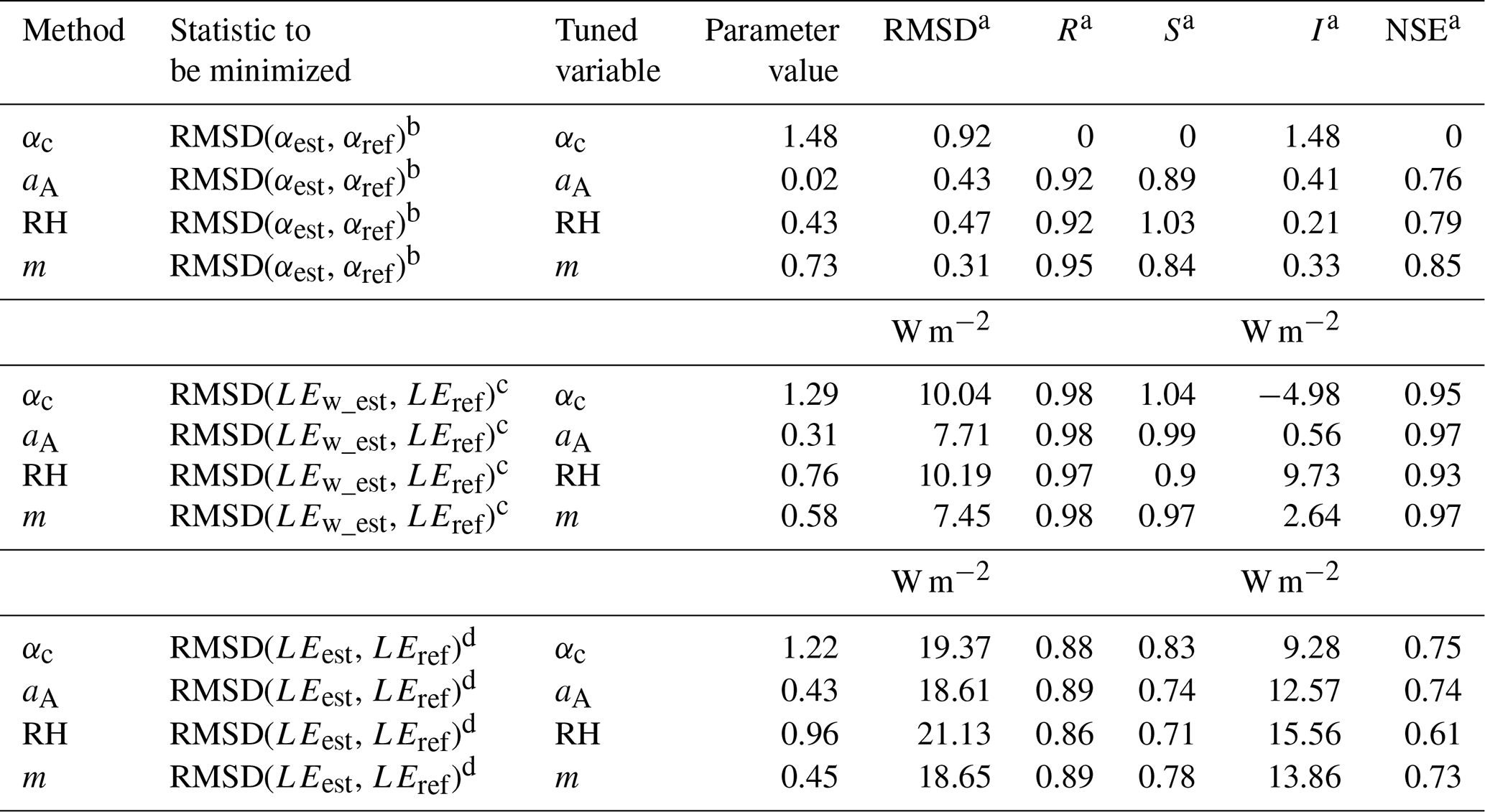
^a RMSD: root mean square difference. R: correlation coefficient. Slope and intercept: S and I in $L{E}_{\mathrm{p}}=S\times L{E}_{\mathrm{ref}}+I$. NSE: Nash–Sutcliffe (1970) efficiency.
^b RMSD(α_est, α_ref) is the RMSD between α estimates found with the prescribed method and the reference values found from α_ref= $L{E}_{\mathrm{ref}}/L{E}_{\mathrm{e}}$ for times with wet-surface evaporation conditions.
^c RMSD(LE_{w_est}, LE_ref) is the RMSD between LE_est estimates found with the prescribed method and the reference values LE_ref for times with wet-surface evaporation conditions.
^d RMSD(LE_est, LE_ref) is the RMSD of all wetness conditions between estimates LE_est and LE_ref.

5 Discussion

5.1 General trends

For convenience, the use of α with a single global value will be called the “α_c method” (corresponding to Hypothesis 1), with (8) it will be the “a_A method” (Hypothesis 2), with Eq. (9) it will be the “RH method” (Hypothesis 3), and with Eq. (11) it will be the “m method” (Hypothesis 4). After discussing trends found in the results, the four hypotheses will be evaluated based on the results.

Figure 1 shows that LE_ref and LE_p (Eq. 1) are very similar when the threshold for wet surfaces at a monthly timescale is taken to be T= $L{E}_{\mathrm{ref}}/L{E}_{\mathrm{p}}=$ 0.90. For daily data the same threshold provides good results, with low rms error and linear regression close to the 1 : 1 line (Table 1), so $L{E}_{\mathrm{ref}}/L{E}_{\mathrm{p}}>\mathrm{0.9}$ was chosen as the indicator of wet-surface evaporation, with no upper threshold to $L{E}_{\mathrm{ref}}/L{E}_{\mathrm{p}}$. Figure 2 shows the geographical location of sites that had some wet-surface evaporation months (upper panel) and sites that did not (bottom panel).

Figure 3 gives the results from the four methods in terms of prediction of α_ref itself (Fig. 3a) and of wet-surface evaporation estimates from Eq. (5) (Fig. 3b). Results from the use of the four methods when used in the CR model y=X are shown in Fig. 4. Even when estimates of α differ considerably from the reference values (Fig. 3a), the methods still provide good estimates of wet-surface evaporation (LE_w – Fig. 3b) and actual evaporation (Fig. 4).

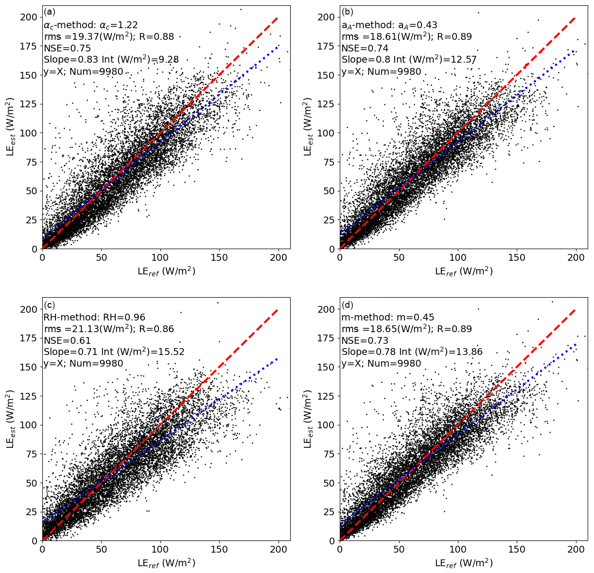
Figure 4 Results for monthly estimates of LE_ref using the CR. Panel (a) uses the α_c method, (b) the a_A method, (c) the RH method, and (d) the m method. Parameter values and statistics are included at the top of each graph. rms is the root mean square error; R is the correlation coefficient; NSE is the Nash–Sutcliffe (1970) efficiency; and Slope and Int are the coefficients in the linear regression equation y= Slope × x+ Int, where x is LE_ref, and y is LE_est. “Num” is the number of data points included. All IGBP classes that are in the dataset are included. The dashed red line is the 1 : 1, and the dotted blue line is the linear regression.

Table 2 provides much of the same data as Figs. 3 and 4 (for monthly averaging), while Table 3 provides the same information for daily averaging. A large number of FLUXNET sites spanning a wide range of climates and land cover classes were included in this study; such a diverse and large number of sites provides some confidence that the trends discussed here would apply to other sites and regions.

Different tuned parameter values were found to calculate α_est (Fig. 3a), LE_PT (Fig. 3b), and LE_est (Fig. 4). Ideally, the tuned parameter values would remain nearly identical in the three cases. A likely explanation for this difference is as follows: in the top panel of Fig. 3, all α_ref values count equally in determination of tuned parameter values that produce the best-fit α_est for each of the methods. But in the bottom panel of Fig. 3, α_est values that correspond to small values of (R_n−G) have far less influence on the RMSD of LE_PT than those corresponding to larger R_n−G. If $R_{\mathrm{n}}-G=$ 5 W m⁻², an increase in α from 1.1 to 1.3 only increases α(R_n−G) from 5.5 to 6.5 W m⁻², whereas if R_n−G is 200 W m⁻², it increases from 220 to 260 W m⁻²; therefore the larger R_n−G would influence RMSD of LE_PT more. Similarly, when moving to the CR estimate LE_est in Fig. 4, the CR estimates again apply different weight to the various estimates of α; therefore different tuned parameter values result here as well. Actually, Brutsaert (2023, p. 149) treats the parameter α in Eq. (5) as a completely different parameter from the α embedded in Eq. (17). While the present authors consider both to be the same parameter, we recognize that its tuned value could vary depending on the context.

For reference, when the parameter values used in Fig. 3b are used in the CR (namely α= 1.29 for the α_c method, α_A= 0.31 for the α_A method, RH = 0.76 for the RH method, and m= 0.58 for the m method), rms errors increased (from 19.37 to 20.12, from 18.61 to 19.25, from 21.13 to 26.84, and from 18.65 to 19.29, respectively). Note that the α_A and m methods still provide the lowest RMSD values.

Figure 3 and Tables 2 and 3 provide evidence that all four methods provide acceptable estimates of actual wet-surface evaporation rates. But what about estimation of hypothetical wet-surface evaporation rates? Szilagyi and Jozsa (2008) and Szilagyi and Schepers (2014) have provided good evidence that a small wet patch within a drying region with wind speed and available energy held constant should maintain a constant surface temperature. The use of Eq. (12) to get the temperature of an actually saturated region is straightforward. Crago and Qualls (2021), Qualls and Crago (2020), and Szilagyi (2021) show graphically, using e–T graphs, how air and ground-surface isenthalps (lines of constant available energy on a (T, e) graph) can be determined, and they show that T₀ is simply the intersection of the ground-surface isenthalp with the saturation vapor pressure curve.

Table 3 Summary of results for daily data (22 998 wet-surface days; 276 020 total days).

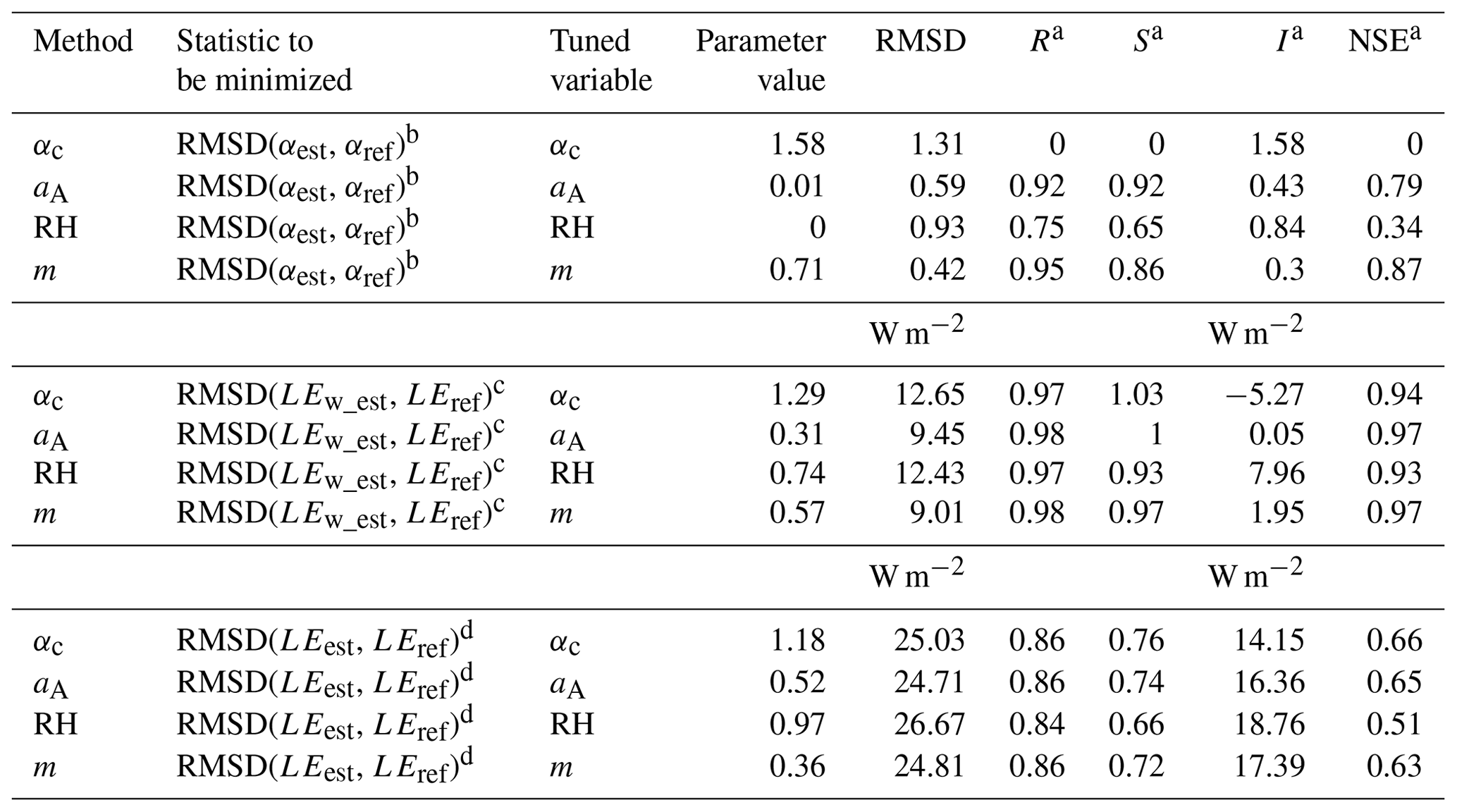
^a RMSD: root mean square difference. R: correlation coefficient. Slope and intercept: S and I in $L{E}_{\mathrm{p}}=S\times$ LE_ref+I. NSE: Nash–Sutcliffe (1970) efficiency.
^b RMSD(α_est, α_ref) is the RMSD for between α estimates found with the prescribed method and the reference values found from α_ref= $L{E}_{\mathrm{ref}}/L{E}_{\mathrm{e}}$ for times with wet-surface evaporation conditions.
^c RMSD(LE_{w_est}, LE_ref) is the RMSD for between LE_est estimates found with the prescribed method and the reference values LE_ref for times with wet-surface evaporation conditions.
^d RMSD(LE_est, LE_ref) is the RMSD for all wetness conditions between estimates LE_est and LE_ref.

There are three distinct explanations for why a best-fit estimate LE_est using the CR (17) might differ from the LE_ref values: first, α may not be estimated correctly (see the preceding paragraphs); second, the LE_PT estimate may not adequately represent the hypothetical wet-surface evaporation rate; and third, the CR formulation may be inadequate. No method to distinguish the effects of these is apparent; therefore the results in Fig. 4 and Tables 2 and 3 only provide an indirect test of the adequacy of the four methods to estimate α for hypothetical wet surfaces.

Under drying surface conditions, since the wet-surface temperature remains constant during drying (assuming R_n−G and wind speed are constant – see Szilagyi and Schepers, 2014), T₀ found with Eq. (12) under drying conditions should still be the correct wet-surface temperature, that is, the temperature at which Δ in Eq. (5) should be evaluated to estimate the hypothetical wet-surface evaporation rate (but note that Δ in Eq. (1) is always taken at air temperature). During the regional drying process, Crago and Qualls (2021) showed that e_a slides down the air isenthalp as drying progresses, while T₀ is found just as it would be for a saturated surface, namely using Eq. (12). So, use of Eq. (12) to determine T₀ for either saturated or unsaturated surfaces seems to have good support, and this T₀ value can be used to predict wet-surface evaporation rates from Eq. (5) with Eq. (4). The process is described above as a temporal drying of the region, but the analysis of Crago and Qualls (2021) is only concerned with the current status of the land and lower atmosphere and not with the drying or wetting pathway to that status.

With respect to the best formulation for the CR, there is unfortunately no consensus (e.g., Crago et al., 2022; Han and Tian, 2018). However, with FLUXNET data from Australia, Crago et al. (2022) found that the y=X formulation was the best overall for predicting latent heat fluxes under many conditions. Given the wide range of methods represented in Figs. 3 and 4, it is actually striking how little variation there is among the various methods with respect to RMSD (Fig. 4; Tables 2 and 3).

Comparison of the four methods associated with hypotheses 1–4 suggests that all the hypotheses can give good estimates in many cases. In Sect. 5.2 we will compare the methods in the context of an examination of these hypotheses.

5.2 Examination of the hypotheses

As discussed in Sect. 1, the objective of this study is to evaluate different hypotheses or conceptualizations regarding α, by using them to estimate α itself, actual wet-surface evaporation (Eq. 5), and hypothetical wet-surface evaporation as a part of a CR model that predicts actual regional evaporation rates (Eq. 17). As discussed in Sect. 5.1, outcomes from these conceptualizations are used to evaluate the hypotheses stated in the Introduction. Including a range of hypotheses in this process makes it more likely that the correct conceptualization will be included and identified as the best.

Hypothesis 1, based on the α_c method, has been the default hypothesis in the majority of work with Eq. (5) and within CR formulations (e.g., Brutsaert, 2015, 2023, p. 148; Crago et al., 2016, 2022). Growing evidence that wet-surface, minimal-advection α actually has a fairly wide range of values (e.g., McNaughton and Spriggs, 1989; Lhomme, 1997a, b; Raupach, 2000) might raise doubt regarding our ability to accurately estimate wet-surface evaporation. Clearly, unexplained variability is a real challenge, but the α_c estimate performs quite well in predicting actual wet-surface evaporation and in the CR model (Figs. 3 and 4 and Tables 2 and 3).

A possible explanation for this surprisingly good performance begins with work by Szilagyi et al. (2014) and Andreas et al. (2013), who showed that much of the variability of α is due to temperature, with α increasing with decreasing temperature. Several formulations for α in terms of temperature are given in Fig. 5, including α_A, α_m, α_max (defined in the Fig. 5 caption), and a multi-term polynomial developed by Szilagyi et al. (2014) for α over saturated land surfaces. Because α is a function of temperature, it is likely that many of the large values of α_ref in Fig. 3a correspond to cold temperatures, which typically imply low available energy. Because available energy is small, relatively large errors in α result in only small absolute errors in wet-surface evaporation using Eq. (5). Thus, the fact that the global constant value of α is too small for these low-temperature sites does not result in large absolute errors in wet-surface evaporation rates. Nevertheless, this is clearly not the best supported of the four hypotheses.

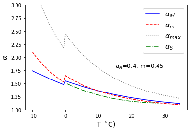
Figure 5 Variability of α from Eqs. (8) and (9) with wet-surface temperature. The value a_A= 0.4 was chosen because it was recommended by Andreas (2013); the value of m= 0.45 was chosen to approximately mimic the trends with the Andreas method. Here ${\mathit{\alpha }}_{\max }=\mathrm{1}+\mathit{\gamma }/{\mathrm{\Delta }}_{T_{\mathrm{0}}}$, the maximum value of α suggested by Priestley and Taylor (1972). The dashed–dotted green line is α_S, based on the third-order polynomial suggested by Szilagyi et al. (2014), on the basis of their analysis of ERA-Interim data over saturated surfaces.

Hypothesis 2, based on the α_A method, assumes a constant ratio (a_A) of the Bowen ratio between equilibrium and minimal-advection conditions. The resulting equation for α (Eq. 8) is able to account for much of the systematic variability of α_ref due to temperature variability because of the variable ${\mathrm{\Delta }}_{T_{\mathrm{0}}}$ in Eq. (8). Figure 3a shows that α_A estimates of α do increase as α_ref increases, but not as quickly as the reference values. While the trend is not matched perfectly, the α_A method is clearly an improvement over the α_c method in terms of predicting α_ref. The method also performs well at predicting actual wet-surface evaporation and actual evaporation (Figs. 3b and 4), and it provides the smallest RMSD for estimating actual evaporation from Eq. (17) for both monthly (Table 2) and daily (Table 3) data. With a clear definition and consistently good performance, Hypothesis 2 has considerable support. However, it is not obvious (based on physical principles) why a_A in Eq. (7) ought to be a constant. Overall, Hypothesis 2 gains considerable support from the data presented here.

Hypothesis 3, based on Eq. (9), also captures much of the variability of α_ref. Equation (9) is correct to within the accuracy of Penman's (1948) well-known assumption regarding Δ, provided that RH is the actual measured relative humidity. When measured RH is replaced with the parameter RH, Eq. (9) provides an estimate for α_ref. Based on Eq. (1) combined with Eq. (5), Eq. (9) suggests that the optimal value of RH should ideally represent the relative humidity that characterizes wet-surface evaporation with minimal advection. Note that in Eq. (9), α depends on f(u), R_n−G, and temperature.

As seen in Tables 2 and 3, the RH method does not rank highly for prediction of α, wet-surface evaporation, or actual evaporation. Hypothesis 3 makes a very intuitive claim regarding wet-surface minimal-advection evaporation, namely, that it is associated with a particular value of relative humidity. While this method is conceptually appealing, and it performs relatively well with some subsets of the data (not shown), its performance in this study is not as good as that of hypotheses 2 and 4. Thus, this study does not provide much support for Hypothesis 3.

Hypothesis 4 assumes that minimal advection has been achieved when α is a specified fraction (m) of the distance from α= 1 to the maximum physically realistic value of ${\mathit{\alpha }}_{\max }=\mathrm{1}+\mathit{\gamma }/{\mathrm{\Delta }}_{T_{\mathrm{0}}}$ (Priestley and Taylor, 1972). The idea of m being this fraction is clear and understandable, but it is not immediately obvious that it must be true on physical grounds. Overall, this method gives the lowest rms error for estimating α and LE_w, it performs nearly as well as the αA method in estimating LE using the CR (Eq. 17), and it does this at both monthly and daily timescales. Furthermore, the other statistics included in Tables 2 and 3 are consistently favourable for this method. The data examined here seem to provide support for this method comparable to the α_A method.

Note that another hypothesis was considered for inclusion, based on the α_S curve, developed by Szilagyi et al. (2014) for saturated land surfaces and included in Fig. 5. The fact that α is a strong function of temperature is an important insight. However, the valid temperature range of their curve is more limited (from 0 to 28^∘) than the temperatures in the dataset, and variability of α with temperature is already included in hypotheses 2, 3, and 4. Also, these hypotheses can be stated in terms of the parameters a_A, RH, and m, respectively, which have well defined and physically meaningful definitions. Therefore, no fifth hypothesis was evaluated.

Different data points might be assumed to represent wet-surface conditions depending on the threshold value of T as illustrated in Fig. 1. But different points could also result for a given T value for different values of z₀ used in the wind function (Eq. 3). The data presented here have used the Wang et al. (2020) z₀ and d₀ formulations as described above. But eddy covariance measurements of friction velocity u^* (m s⁻¹) are available for most of the sites and measurement periods. This means the logarithmic wind profile $u=(u^{*}/k$)log[($z_u-d_{\mathrm{0}})/z_{\mathrm{0}}$] (e.g., Brutsaert, 2023, p. 41) can be solved for z₀ for each measurement period for which u^* is available. This value of z₀ is specific to a particular site and a particular month or day, so it accounts for roughness variations with season and wind direction. With these data, the values of z₀ calculated in this way are somewhat smaller than those found with the Wang et al. (2020) formulation, which causes LE_p values to be smaller and more data points to be identified as wet-surface values. Nevertheless, a figure similar to Fig. 1 but using these new z₀ values (not shown) suggests that T= 0.9 is still appropriate. This method results in root mean square differences (see the Supplement, Tables S2 and S3) comparable to those in Tables 2 and 3. The number of data points differ because not all time periods had u^* measurements and because different z₀ values resulted in different data points qualifying as wet-surface values. However, the key points remain unchanged. Results from the Wang et al. (2020) version of z₀ and d₀ are shown herein because they represent the way the roughness of land surfaces is usually estimated.

6 Conclusions

Four hypotheses regarding the Priestley–Taylor (1972) parameter α were considered. Each of them has a different assumption regarding the nature and variability of α. In the first hypothesis α is constant; in the second it represents a ratio of two Bowen ratios; in the third, it represents conditions at a given relative humidity value; and in the last, it can be seen as a midpoint between theoretical maximum and minimum values. Using FLUXNET data from a total of 171 stations, α, LE_PT, and actual evaporation values are compared to reference values in an attempt to determine which hypotheses best explain the data.

The second and fourth hypotheses generally produce the best results. In both of these, α is dependent on temperature, although the functional forms of the relationship are different. The third hypothesis has a very intuitive physical interpretation, but it tends not to work as well as the α_A and m methods. But overall, the data in this study provide the most support for hypotheses 2, the α_A method, and 4, the m method. According to Hypothesis 2, the actual Bowen ratio under wet-surface conditions with minimal advection is a constant fraction of the Bowen ratio under equilibrium conditions (Eq. 4). According to Hypothesis 4, α for wet surfaces remains at a constant fraction (m) of the distance between the minimum of value of 1 and the maximum value of $\mathrm{1}+\mathit{\gamma }/{\mathrm{\Delta }}_{T_{\mathrm{0}}}$. Since ${\mathrm{\Delta }}_{T_{\mathrm{0}}}$ is a function of the wet-surface temperature T₀, so is α_m.

Without a need for any additional data, the temperature dependence of α can be included in evaporation equations. It seems appropriate to include this dependence in applications of the Priestley–Taylor (1972) equation and in particular in the use of CR models to estimate actual evaporation over drying surfaces. It is striking that four distinct hypotheses for how to understand the physical meaning of α can be stated clearly and that they have real implications regarding the nature and the numerical value of α.