the Creative Commons Attribution 4.0 License.
the Creative Commons Attribution 4.0 License.
 | 12 Jan 2023
The effects of rain and evapotranspiration statistics on groundwater recharge estimations for semi-arid environments
Tuvia Turkeltaub
Golan Bel
A better understanding the effects of rainfall and evapotranspiration statistics on groundwater recharge (GR) requires long time series of these variables. However, long records of the relevant variables are scarce. To overcome this limitation, time series of rainfall and evapotranspiration are often synthesized using different methods. Here, we attempt to study the dependence of estimated GR on the synthesis methods used. We focus on regions with semi-arid climate conditions and soil types. For this purpose, we used longer than 40 year records of the daily rain and climate variables that are required to calculate the potential evapotranspiration (ETref), which were measured in two semi-arid locations.These locations, Beit Dagan and Shenmu, have aridity indices of 0.39 and 0.41, respectively, and similar seasonal and annual ETref rates (1370 and 1030 mm yr−1, respectively) but different seasonal rain distributions. Stochastic daily rain and ETref time series were synthesized according to the monthly empirical distributions. This synthesis method does not preserve the monthly and annual rain and ETref distributions. Therefore, we propose different correction methods to match the synthesized and measured time series' annual or monthly statistics. GR fluxes were calculated using the 1D Richards equation for four typical semi-arid soil types, and by prescribing the synthesized rain and ETref as atmospheric conditions. The estimated GR fluxes are sensitive to the synthesis method. However, the ratio between the GR and the total rain does not show the same sensitivity. The effects of the synthesis methods are shown to be the same for both locations, and correction of the monthly mean and SD of the synthesized time series results in the best agreement with independent estimates of the GR. These findings suggest that the assessment of GR under current and future climate conditions depends on the synthesis method used for rain and ETref.
- Article
(3057 KB) - Full-text XML
-
Supplement
(1623 KB) - BibTeX
- EndNote


Rainfall characteristics such as total amount, intensity, and frequency are important climate factors that strongly influence groundwater recharge (GR) rates (Small, 2005; Nasta et al., 2016; Barron et al., 2012). Understanding the effects of climate variables on the GR is essential for both a fundamental understanding of the physical processes and for the groundwater management under future climate conditions. Various studies have illustrated that rain intensity is superior to the total annual rainfall in determining GR (e.g., Ng et al., 2010; Owor et al., 2009). Previous studies in semi-arid areas illustrated that coarser soils facilitate higher recharge rates than finer soils (Keese et al., 2005; Wohling et al., 2012; Crosbie et al., 2013). These studies presented statistical relationships between annual rainfall and GR for each of the reported soil types (sand, loam, and clay loam) or according to clay content. However, it has been demonstrated that using annual rainfall may yield large uncertainties in recharge estimations due to seasonal effects (Small, 2005; Cuthbert et al., 2019; Moeck et al., 2020). Small (2005) illustrated that, in sandy and sandy loam soils, seasonal rainfall variations have a stronger effect on recharge than storm size distribution. An additional factor that may impede establishing a relationship between rain and recharge is the thickness of the unsaturated zone. Many semi-arid and arid areas across the world are characterized by a thick unsaturated zone (> 15 m), where water travel times can be on the order of years or decades (Gurdak et al., 2007; Scanlon et al., 2009; Fan et al., 2013; Turkeltaub et al., 2015; Cao et al., 2016; Turkeltaub et al., 2018; Moeck et al., 2020; Turkeltaub et al., 2020). Current historical rain records are not long enough to enable a complete characterization of the relationship between rain characteristics (number of rainy days, storm duration, rain intensity, etc.) and GR in semi-arid and arid areas. In order to overcome this limitation, assuming that the rain characteristics do not change over the period of interest, long rain time series can be generated (synthesized) from the statistics of the measured rain (Rodriguez-Iturbe et al., 1999; Small, 2005).
To generate synthetic rain, the statistics of both the rain occurrences and the rain intensities must be defined (Tencaliec et al., 2020). The number of rain events is a discrete variable, while the amount of rain in each event is a continuous one. Thus, different models/distributions are implemented to describe each of the components yielding the rain series (Tencaliec et al., 2020). Previous studies that analyzed the relationship between rain statistics and GR used the Poisson approach to generate synthetic rain (Rodriguez-Iturbe et al., 1999; Small, 2005; Burton et al., 2008). In general, an exponential distribution is used to describe the distribution of dry intervals between sequential rainfall events, the storm depth (total amount of rain in the storm), and the rain rate (Small, 2005). In order to preserve the seasonal or annual means, the parameters of the different distributions (i.e., the distributions of the dry/wet intervals and rain intensity) are assumed to be dependent such that the means of interest are conserved (Istanbulluoglu and Bras, 2006). Note that this implies replacing correlated variables with independent ones that include parameters that are not derived from the measurements. To include the seasonal rain distribution, the parameters of the exponential distributions must be defined for each month or by simply dividing the year into two seasons, dry and wet (Snyder et al., 2003; Small, 2005). Other studies suggested using a nonstationary Markov chain or a Bernoulli distribution to describe the occurrence of rain and gamma distributions to describe the rainfall amounts (Stern and Coe, 1984; Lima et al., 2021). These methods suffer from an overparameterization or an underestimation of rain amounts (Snyder et al., 2003; Tencaliec et al., 2020).
While the effect of rain statistics on GR has received much attention, knowledge concerning the impact of the potential evapotranspiration (ETref) statistics on GR fluxes is limited. It was previously demonstrated that GR may decrease despite an increase in the total annual rain (Rosenberg et al., 1999; Kingston and Taylor, 2010). This was attributed to increases in monthly temperature, which, in turn, increases the monthly potential and actual ET rates. Small (2005) generated ETref time series by accounting for the ETref mean annual value and seasonal amplitude. It was found that the synchronization (or lack of it) dictates the GR amounts. However, previous studies have shown that a reliance on monthly or annual means of meteorological variables may lead to a bias in GR predictions (Wang et al., 2009; Batalha et al., 2018).
The current study aims to identify the important characteristics of the local rain and ETref for estimating the diffuse recharge under semi-arid climate conditions. Specifically, we test the sensitivity of estimated GR fluxes to the daily, monthly, and annual statistics of rain and ETref. Relatively long rain and Penman–Monteith ETref records (> 40 years) in two different locations with different seasonal rainfall patterns but comparable ETref rates are used to generate synthetic daily rain and ETref time series. These time series preserve the daily statistics but not necessarily the other characteristics of the rain and ETref. To overcome this issue, several new methods (see the Methods section for detailed descriptions) that preserve different characteristics of the measured rainfall and ETref records are applied, and the different synthetic data series are used to assign the atmospheric boundary conditions for GR simulations. Recharge fluxes are simulated by solving the Richards equation with different hydraulic parameters corresponding to typical semi-arid soil types. These soil parameters were selected according to the global distribution of the soil texture in semi-arid and arid environments. Ultimately, the effects of the seasonal rain distribution and the synthesis methods on the estimated GR fluxes are discussed. Note that we focus on the simpler case of bare and homogeneous soil. Estimations of actual GR fluxes in the presence of vegetation and preferential flow require specific field details and are beyond the scope of the current study.
2.1 Climate data
The meteorological datasets used in this study were obtained at the Beit Dagan (32∘00′ N, 34∘49′ E, 30 m a.m.s.l.) and Shenmu (38∘55′ N, 110∘7′ E, 926 m a.m.s.l.) meteorological stations. These stations were selected for their similar seasonal and annual Penman reference evapotranspiration (ETref) (Allen et al., 1998) rates. However, their annual and seasonal rainfall distributions are different (Fig. 1).
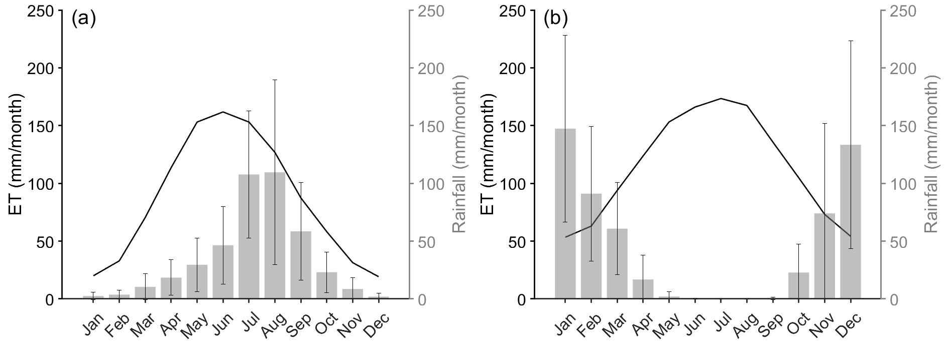
Figure 1Climate data from meteorological stations located in (a) Shenmu, Loess Plateau, China, and (b) Beit Dagan, Israel. The climate data are presented as mean and SD perennial monthly values (the original data were measured at daily resolution).
According to the meteorological climate records, the Shenmu site is characterized as a semi-arid temperate location with mean, maximum, and minimum annual temperatures of 9, 16, and 3 ∘C, respectively. The mean annual precipitation is 420 mm, with approximately 70 % of it falling between June and September (in summer; mostly monsoon rain). This implies that the rainy season corresponds to the months with the largest ETref rates. Maximum and minimum ETref rates occur during June (5.4 mm d−1) and December (0.6 mm d−1), respectively. Beit Dagan represents a Mediterranean climate, where winter is the rainy season (October to March), implying that the rainy season corresponds to the period with the lowest ETref rates. The mean, maximum, and minimum annual temperatures are 19, 31, and 7 ∘C, respectively. The mean annual precipitation is 553 mm yr−1. Maximum and minimum ETref rates occur during July (5.9 mm d−1) and January (1.8 mm d−1), respectively.
The dataset for Beit Dagan spans 57 years of records (1964–2021), and the dataset for Shenmu spans 54 years of records (1961–2014). Both records are considered long enough to represent the natural climate variability (Döll and Fiedler, 2008). The climate datasets contain daily measurements of mean air temperature (∘C), maximum temperature (∘C), minimum temperature (∘C), precipitation (mm), relative humidity (%), sunshine hours (h), and wind speed (m s−1). Using these datasets, the daily ETref rates were calculated according to the Penman–Monteith equation (Allen et al., 1998) for each meteorological station (see Fig. 1 for the precipitation and ETref data; note that, due to the lack of solar radiation measurements, we used the Angstrom formula, which relates solar radiation to extraterrestrial radiation and relative sunshine duration Allen et al., 1998). Note that 3237 d of the ETref in Beit Dagan are missing, with the longest gap occurring between 22 March 2008 and 31 December 2014. The data were used to derive the empirical probability distribution function (ePDF) of the variables. Therefore, we did not need to extrapolate the missing values, and the ePDFs are based only on the existing data.
In addition to the measured data, we also used the CRU TS 3.2 dataset (Harris et al., 2014), which was downscaled to daily values with ERA40 (1958–1978, Uppala et al., 2005) and ERA-Interim (1979–2015, Dee et al., 2011). The downscaling method is described more extensively in van Beek (2008).
2.2 Generation of the rain and ETref time series
The measured rain (MR) records were analyzed for each calendar month separately. For each month, we derived the distribution of the number of rainy days and the distribution of the daily rain amount. We used these observation-based empirical distributions with no fitting. The synthetic rain was generated for each month according to these two characteristics. First, the number of rainy days (obviously an integer number) was drawn, and then, for each day, the amount of rain was assigned (a number drawn from a continuous probability distribution). Using this method to generate the synthetic rain, we conserved the daily rain statistics (hereafter denoted as DS). In order to assess the importance of the distribution of the number of rainy days in each month, we also generated synthetic rain time series, where we used the average number of rainy days for each month, i.e., a fixed number of rainy days (the synthetic rain generated using this method is hereafter denoted as FNRD). The amount of rain in each of these days was drawn from the corresponding distribution of the daily rain amount. In order to illustrate the importance of the fact that the rain is limited to a certain number of days, we also considered a scenario in which the total monthly rain generated using the DS method was spread equally over all the days of the month. This scenario is hereafter denoted as UDDS.
However, the above procedures do not account for the correlation between the number of rainy days and the total amount of rain in the month, nor for the correlations between the rain amounts within successive months. Therefore, we adopted several methods to correct the daily rain amounts, as detailed below. The first correction method aimed at correcting the daily rain amounts such that the monthly averages and standard deviations (SDs) of the synthetic rain and the measured rain are the same for each calendar month. This method is denoted as monthly corrected daily statistics (MCDS). Practically, the correction was applied by considering the DS rain series and multiplying each value in this series by the ratio between the measured SD of the total monthly rain and the SD of the total monthly rain of the synthesized DS series for the corresponding calendar month. Next, we added to each value in the synthetic series the difference between the measured and synthetic monthly means divided by the number of rainy days in that month. Note that this correction could possibly have resulted in negative rain amounts; therefore, we only considered the rainy days with amounts above the correction in order to ensure positive values of rain amounts and to conserve the number of rainy days. Mathematically, this correction method is described as
Here, is the amount of rain in year y, month m, and day d of the corrected synthetic rain series. is the amount of rain in year y, month m, and day d of the DS rain series. is the difference between the measured and the DS monthly rain averages for month m. The averages are defined as
where Ny is the number of years spanned by the record. The average synthetic monthly rain is defined similarly. Nm(y,m) is the number of rainy days in month m of year y with a rain amount large enough such that mm if the correction is applied. If this is not the case, the amount of rain remains equal to its value in the DS series. and are the SDs of the total monthly rain for the DS series and the measured rain of the calendar month m, respectively. The SD of the measured monthly rain is
In the second method, we applied a similar correction to the DS series, but rather than conserving the monthly mean and SD, we conserved the annual mean and SD. Mathematically, this correction may be written as
is the difference between the measured and the DS annual rain averages. The annual averages are defined as
and similarly for the DS series. The SD of the measured annual rain is
and similarly for the DS series. It is important to note that in both the MCDS and ACDS corrections, we ensured that on each rainy day, there is at least 1 mm of rain, and we conserved the rainy days (namely, each rainy day in the DS series is also a rainy day in the MCDS and ACDS series).
Three methods similar to those described above for the rain synthesis were used to establish the synthetic ETref time series. The first method was similar to the DS method, where empirical probability density functions were established from the daily ETref records for each calendar month separately. Subsequently, the synthetic ETref time series were created by the random sampling of ETref values from the corresponding empirical distributions. This method is hereafter denoted as ETDS. The other two methods involve corrections of the ETDS series. The ETDS time series were corrected to monthly (ETDSMC) and yearly (ETDSAC) statistics, similarly to the abovementioned procedure (see Eqs. 1–6). Additional ETref synthesis methods involve establishing the empirical density functions of ETref for rainy and dry days separately for each calendar month. The ETref values in the synthetic series are sampled from the corresponding empirical distribution according to the rainy and dry days in the synthetic rain series. Namely, if the synthetic rain series shows rain on the specific day, the synthetic ETref value is randomly sampled from the empirical distribution of ETref values for rainy days in the corresponding calendar month. If the synthetic rain series shows no rain on that day, the synthetic ETref value is randomly sampled from the empirical distribution of ETref values for dry days in the corresponding calendar month. This method is hereafter denoted as ETWD. Here as well, the ETWD time series were corrected to conserve the monthly (ETWDMC) and annual (ETWDAC) statistics of ETref. The last ETref synthesis method was mostly used as a reference to demonstrate the importance of the daily values’ statistics. In this method, the daily values for each calendar month throughout the entire record for each station were averaged, and ETref was assumed to be constant (equal to the average value for the corresponding calendar month) for each calendar month. This method is hereafter denoted as ETUD.
In the Supplement, comparisons between the cumulative distribution functions (CDFs) of the measured and synthesized daily rain, the number of rainy days, and the daily ETref values in each calendar month are presented. The two-sample Kolmogorov–Smirnov test indicated that the synthesized and the measured distributions are statistically similar for the DS, ETDS, and ETWD methods (see Table S1). Implementing the different methods allowed us to examine the sensitivity of the GR to the different statistical characteristics of the rain and the ETref. For convenience, Table 1 provides a detailed list of all the abbreviations used for the different rain and ETref synthesis methods.
Table 1Description of the abbreviations of the different rain and ETref methods.

For each method, we used 50 different realizations of the synthetic rain series. The variance of the estimated GR includes two components: the temporal variability within each realization of the atmospheric conditions (rain and ETref) and the variability between different realizations. The total variability of the annual GR is defined as
where GR(r,y) is the GR predicted by realization r of the atmospheric conditions for year y, Ny is the number of years for which the GR is predicted, Nr is the number of atmospheric condition realizations, and the average is defined as
It is easy to show that the total variability can be decomposed into the temporal and the realization contributions (e.g., Strobach and Bel, 2017) as
where
and
This decomposition allows us to assess the number of realizations required to estimate the GR variability.
2.3 Model setup
The GR fluxes were calculated using the 1D Richards equation,
where ψ is the matric potential head [L], θ is the volumetric water content (dimensionless), t is time [T], z is the vertical coordinate [L], and K(ψ) [L T−1] is the unsaturated hydraulic conductivity function. The Richards equation was numerically simulated using Hydrus 1D (Šimŭnek et al., 2009). Atmospheric boundary conditions with surface runoff were prescribed at the upper boundary as precipitation, ETref (potential ET), and the minimum allowed pressure head at the soil surface (hCritA cm). The lower boundary conditions were prescribed as free drainage, and the length of the simulated soil column was 500 cm.
Knowledge regarding the soil hydraulic functions is essential in order to solve the Richards equation. The soil retention curves and the unsaturated hydraulic curves are commonly described according to the van Genuchten–Mualem (VGM) model (Mualem, 1976; Van Genuchten, 1980):
where Se is the degree of saturation (), θs and θr are the saturated and residual volumetric soil water contents, respectively, and α [L−1], n, and are shape parameters. Hydraulic conductivity is assumed to behave according to
where Ks [L T−1] is the saturated hydraulic conductivity and l is the pore connectivity parameter, prescribed as 0.5.
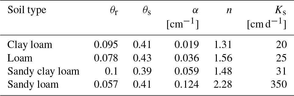
The global distribution of soil texture provided by Hengl et al. (2014) and the aridity definition by the Food and Agriculture Organization (FAO, 2023) were used to determine the common soil types in arid and semi-arid environments (Fig. 2). It was found that 94 % of the soil types in semi-arid and arid regions according to the USGS soil characterization are clay loam, loam, sandy clay loam, and sandy loam (Fig. 2). We used the soil hydraulic parameters provided by Carsel and Parrish (1988) that correspond to each of these soil types (Table 2). Note that only homogeneous soil profiles are simulated in the current study. We mention again that soil heterogeneity, local topography, vegetation, and other complex soil water processes are likely to affect GR estimations. However, these additional complexities have to be analyzed separately and require detailed and location-specific observations.
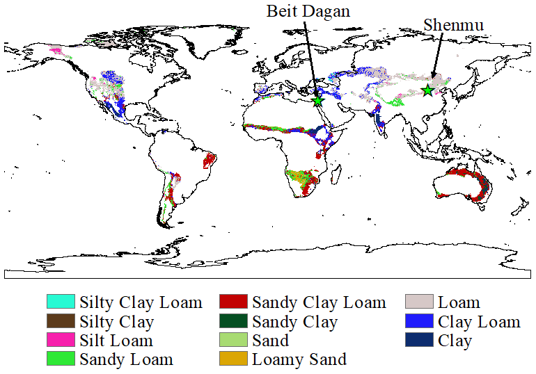
Figure 2Global distribution of soil types in semi-arid and arid regions (the aridity index is between 0.2 and 0.5) according to the Food and Agriculture Organization (FAO, 2023), and the spatial soil texture distribution in these regions as provided by Hengl et al. (2014).
Table 2The soil hydraulic parameters used in the current study. The typical soil types in semi-arid and arid regions were identified according to the analysis presented in Fig. 2. The parameters corresponding to each soil type were derived from the lookup table at Carsel and Parrish (1988).
3.1 Characteristics of the different methods to synthesize the rain and the ETref
Figure 3 shows the monthly rain statistics for each of the rain synthesis methods (DS, MCDS, ACDS, and FNRD). Note that comparisons between the measured and synthetic daily (Figs. S1 and S2) and monthly (Figs. S3 and S4) rain cumulative distribution functions (CDFs) for each rainy month appear in the Supplement. Figures S5 and S6 provide a similar comparison between the distributions of the number of rainy days. In addition, Figs. S7 and S8 compare the measured and synthetic annual rain CDFs.
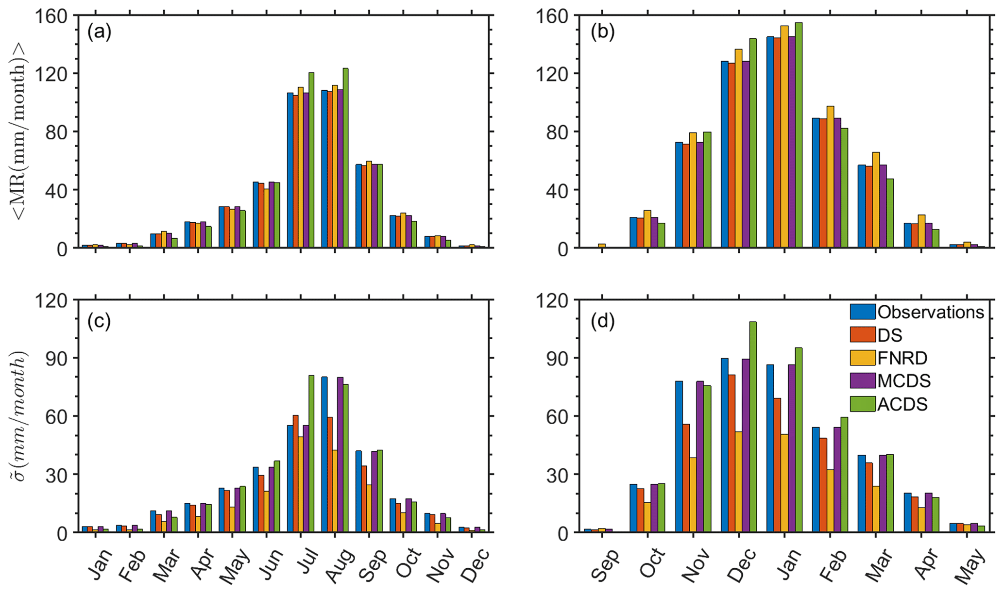
Figure 3(a, b) Mean and (c, d) standard deviation of monthly rain for the (a, c) Shenmu climate and the (b, d) Beit Dagan climate. Note that the colors indicate the method of rain synthesis.
The DS method, which preserves the daily rain statistics and the statistics of the number of rainy days in each month, generates mean monthly rain amounts that are close to the observed values. However, both the monthly mean and the monthly SD () are generally underestimated. This occurs because the correlation between the number of rainy days and the total monthly rain was not accounted for. The FNRD method generates, in most cases, a higher mean monthly rain amount but a lower SD than the DS method (Fig. 3). Again, this is the result of not considering the correlation between the number of rainy days and the total rain amount. Namely, the number of rainy days is fixed, while the statistics of the daily rain amount follow the empirical PDF extracted from the observations. It is apparent that the statistics of the MCDS method are closest to the monthly observations, as expected (Fig. 3). Figures S3 and S4 provide additional presentations of these characteristics by comparing the CDFs of the total monthly rain for each synthesis method and the measurements.
The ACDS method tends to overestimate the mean and SD of the monthly rain during the months with the most rain, while the monthly means are underestimated during the driest months (Fig. 3). This is because the SD correction in this method, which is actually a multiplication by a factor larger than 1, amplifies the large rain events more than the small ones. Note that this correction is needed because the DS tends to underestimate the annual rain amount and SD. Figures S7 and S8 provide additional presentations of these characteristics by comparing the CDFs of the total annual rain for each synthesis method and the measurements.
The monthly statistics of the synthesized ETref generated by ETDS, ETWD, ETDSMC, ETDSAC, ETWDMC, and ETWDAC are depicted in Fig. 4. ETDS and ETWD show mean values that are similar to the observed ones. Both methods underestimate the SD of ETref (see Fig. 4). This underestimation stems from the fact that the daily ETref values for each month are derived from the empirical distribution, which is based on the entire dataset. Therefore, correlations within the month and the variability between years with higher ETref values and those with lower values are not accounted for. In other words, the values of the synthesized ETref in each month mix observed values within this calendar month from different years of the observations. Therefore, the difference between the synthesized mean ETref values for a specific calendar month in different years is smaller than the observed difference. The similarity between the statistics of the two methods suggests that the correlation between the ETref values and the rainy/dry nature of the day is not apparent. We also tested the importance of the ETref trend within the calendar month, and we found that it does not affect the observed statistics.
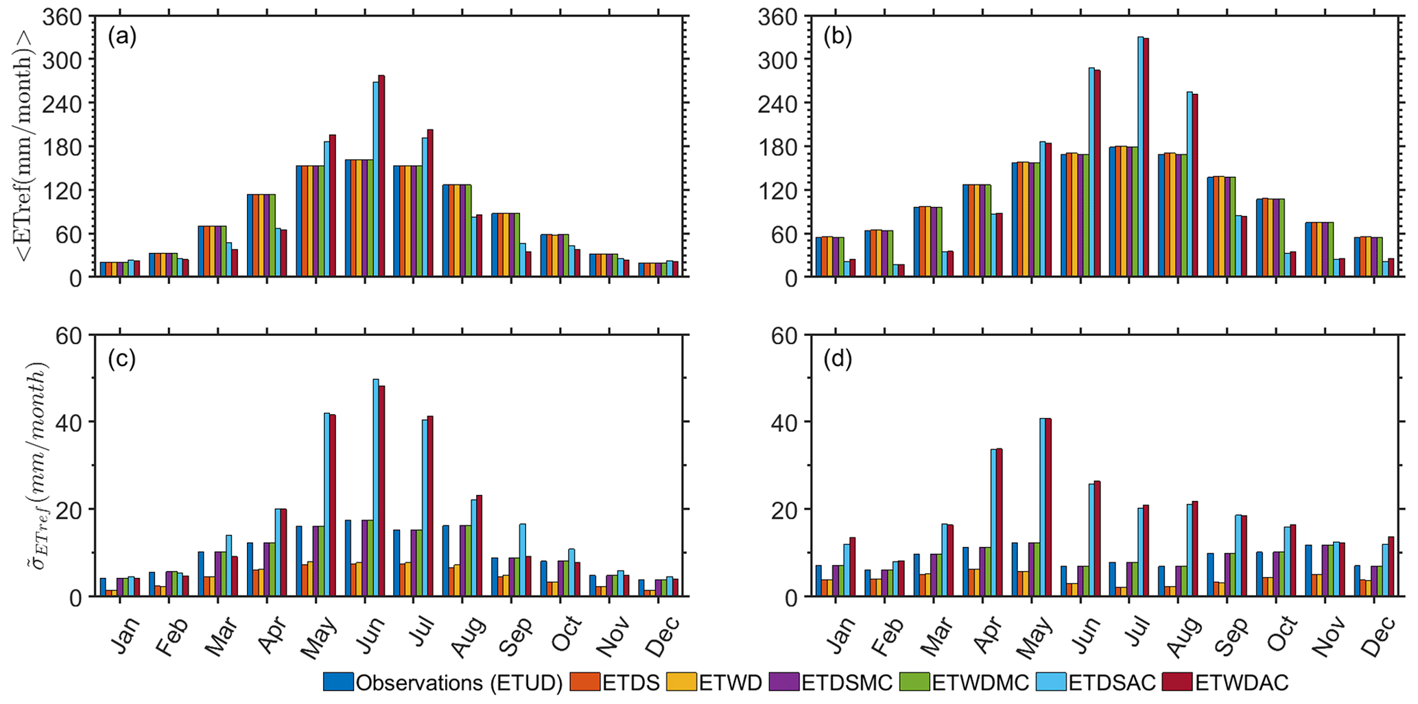
Figure 4(a, b) Mean and (c, d) standard deviation of monthly ETref for the (a, c) Shenmu climate and the (b, d) Beit Dagan climate. Note that the colors indicate the method of ETref synthesis.
Following the monthly corrections (Eqs. 1–3), the monthly mean and SD of the ETref that were synthesized by the ETDSMC and ETWDMC methods match the observed values (Fig. 4). Both methods show very similar results for the mean and SD monthly values (see Figs. S9–S14 for comparisons between the measured and synthetic daily (Figs. S9 and S10), monthly (Figs. S11 and S12), and annual (Figs. S13 and S14) ETref CDFs). This similarity suggests that the correlation between the ETref value and the rainy/dry nature of the day is not very strong. As expected, the mean and SD for both methods are very close to the observed monthly values.
For both the ETDSAC and ETWDAC methods, higher monthly means were calculated during the warm months compared with the observations, while lower values were estimated for the cold months (Fig. 4). Note that the number of rainy days is synthesized for each month separately. Thus, the correlations between the number of rainy days in different months within the same calendar year are not accounted for. This, in turn, results in small differences between the synthesized ETDSAC and ETWDAC SD values.
3.2 A comparison between estimated GR using observed and DS-synthesized climate data series
To better understand the effects of the DS synthesis method, we calculated (using the 1D Richards equation) the GR fluxes under the observed and DS synthesized climate conditions. The calculations were done for both locations, Shenmu and Beit Dagan. In addition, we used the CRU-ST reanalysis data and the corresponding DS synthetic data (the DS in this case was based on the ePDF of the reanalysis data) and repeated the GR flux calculations. The abovementioned estimated GR fluxes are depicted in Fig. 5.

Figure 5Panels (a–d) present the Shenmu (summer rain) estimated GR fluxes and (e–h) present the Beit Dagan (winter rain) estimated GR fluxes. Obs denotes the GR fluxes that were calculated using the observed rain and ETref; CRU_Data denotes the GR fluxes that were calculated using the downscaled CRU TS climate datasets (van Beek, 2008; Harris et al., 2014); DS_Obs denotes the GR fluxes that were calculated using the DS-synthesized rain and ETref that were established according to the observed data statistics; CRU_DS denotes the GR fluxes that were calculated using the DS-synthesized rain and ETref that were established according to CRU TS statistics.
For all the soil types considered, higher annual average (and SD) GR fluxes are estimated when the observed climate data in Shenmu is used (relative to the CRU data; Fig. 5, panels a–d). In Beit Dagan, there is no significant difference in the estimated annual average (and SD) GR fluxes between the observed and CRU data (Fig. 5, panels e–h). The estimated GR fluxes in Shenum (Fig. 5, panels a–d) resemble previously reported GR fluxes in the Loess Plateau. Tao et al. (2021) recently suggested that for loam and sandy clay loam textures (∼ 20 % clay), the GR fluxes range from 24.5 to 33.8 mm yr−1. These values are similar to our results when the observed climate conditions are used and are more than the estimated GR fluxes when the CRU data are used. Other studies suggested a range of 50 to 90 mm yr−1 (Gates et al., 2011; Huang et al., 2017), which is closer to the estimated values in coarser soil textures (sandy loam). Regional analyses showed a larger range of GR flux over the entire Loess Plateau – between 0 and 75 mm yr−1 (Turkeltaub et al., 2018; Hu et al., 2019) – and Wu et al. (2019) reported GR fluxes larger than 100 mm yr−1 for some specific locations, similar to our estimated GR fluxes for sandy loam soil (Fig. 5d). Our estimated GR fluxes for Beit Dagan are also similar to those reported in previous studies. Eriksson and Khunakasem (1969) reported GR fluxes that range between 30 and 326 mm yr−1 along the coastal aquifer of Israel (our results are within this range and are in line with the estimation for the specific soil types considered here). A commonly used recharge coefficient for the Israeli coastal aquifer is about 0.3 of the rainfall (Gvirtzman, 2002). Given that the average rainfall in the region is ∼ 600 mm yr−1, the corresponding average GR flux is about 200 mm yr−1 (similar to the our estimates for the finer soil types). Higher GR rates (330 mm yr−1) were estimated by Turkeltaub et al. (2015) in a site near Beit Dagan, which is characterized by a sandy soil, in agreement with our estimate for the sandy loam. These findings are supported by chloride and water isotope observations (Kass et al., 2005; Rimon et al., 2011). For heavy soils (e.g., clay loam) the range of the GR fluxes is wider and in many cases depends on local vegetation, agricultural activity, and preferential flow through cracks (Kurtzman and Scanlon, 2011; Baram et al., 2012; Kurtzman et al., 2016). We emphasize again that the effects of these factors on GR flux estimations are beyond the scope of this study.
The GR fluxes that were calculated using the DS-synthesized rain and ETref mostly show smaller means and SDs compared with GR fluxes estimated using the observed climate data (Fig. 5). A similar trend is also apparent for the CRU and the corresponding DS-synthesized data. This is an outcome of narrower yearly rain and ETref distributions for the DS-synthesized variables (see Supplement Figs. S7, S8, S13, and S14). The DS method does not account for the correlation between the amount of rain and the number of rainy days or the existence of rainy (dry) years. Similarly, the ETDS method does not account for the inter-annual variability, namely, the existence of warm and cold years. In both methods, the statistics for each calendar month are based on the entire recorded time series and, therefore, the resulting distributions are narrower. This difference between the observed and the DS-synthesized statistics inspires the implementation of various correction methods. However, the choice of the most adequate correction method is not straightforward and will be discussed later on.
3.3 GR estimations using different corrections for the DS synthesis
Groundwater recharge sensitivity to different rain characteristics is examined by constraining the synthesized rain (DS) to yearly or monthly statistics as described in the Methods section. Additionally, the GR fluxes that were calculated when using only an average number of rainy days (FNRD) or when the monthly rain and ET are distributed over the month (UDDS) are compared with the DS method. The estimated GR fluxes are presented as the average annual GR fluxes together with their SDs σtotal (Fig. 6). Note that the symbols represent the soil types, and the colors indicate the ETref methods (Fig. 6). Thus, in total, we used 29 different methods to estimate the GR fluxes for each soil type and climate (Fig. 6).
In general, under both climate conditions, the estimated GR increases in the following order: Clay Loam < Loam < Sandy Clay Loam < Sandy Loam (Fig. 6). Furthermore, the estimated GR fluxes under winter rain are substantially higher than those under the summer rain climate (Fig. 6). When applying the ACDS method, i.e., correcting the synthesized rain to match the recorded yearly statistics, the estimated GR fluxes are considerably higher than those estimated using the other rain synthesis methods (Fig. 6). Using the UDDS method, where both the monthly rain and the ETref are uniformly distributed over the month, resulted in considerably lower GR fluxes compared with the other methods. The estimated GR fluxes using the FNRD have similar mean values and higher SD values relative to the GR fluxes estimated using the DS method (Fig. 6). Therefore, it appears that the distribution of the number of rainy days is not crucial when establishing a rain series for GR studies. The GR fluxes estimated using the MCDS method are slightly larger than those estimated using the DS method.

Figure 6Estimated perennial GR based on 50 realizations for each of the typical soil types for the Shenmu and Beit Dagan climates. The different colors indicate the method of ETref synthesis. Note that the error bars represent the total SD, σtotal.
The ETref synthesis methods preserving the daily (ETDS and ETWD) or monthly (ETDSMC and ETWDMC) statistics and the uniformly distributed ETref (ETUD) result in similar GR fluxes. However, the ETref synthesis methods preserving the yearly statistics (ETDSAC and ETWDAC) result in considerably higher GR fluxes. This effect stems from the fact that these correction methods widen the distribution of the ETref values. However, while smaller values of ETref do indeed decrease the actual evapotranspiration, the much larger values of ETref do not affect the actual evapotranspiration because it already reaches an upper limit. The difference between the ETref values during wet and dry days does not affect the GR fluxes. For all the correction methods, there were no apparent differences between the ETref synthesis methods that account for wet/dry differences and those that do not.
We further investigated whether the number of realizations (50 in the current study) is sufficient to adequately analyze the effects of the rain and ETref synthesis methods on GR fluxes. Both and were calculated for 200, 20, and 10 years according to Eq. (9) (see also Fig. 7). Calculating the ratio between and illustrates that constitutes most of the variability (Fig. 7c, d). These results help confirm that increasing the number of realizations would have little effect on the estimated variance of the GR fluxes and that the number of realizations we used is sufficient.
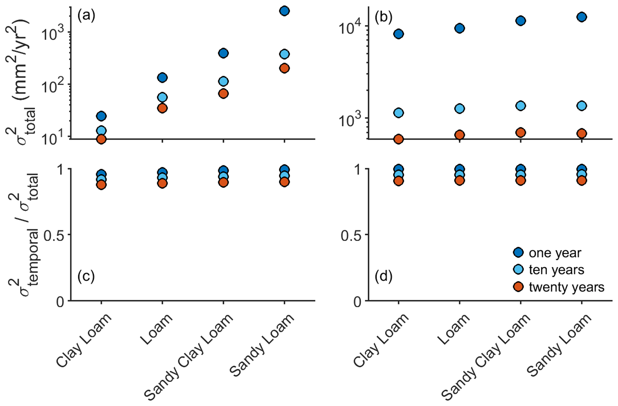
Figure 7Total variance () of the estimated perennial GR for (a) Shenmu and (b) Beit Dagan. The ratio between the internal variance () and total variance () is presented for the (a) Shenmu climate and the (b) Beit Dagan climate.
3.4 Correlation between annual rainfall and annual GR
The relationships between annual rain and annual GR fluxes are commonly used for regional GR estimations (e.g., Wohling et al., 2012) and to test possible future changes in GR fluxes (e.g., Crosbie et al., 2013). Thus, the correlations between annual rain and annual GR fluxes for each combination of soil type, ET synthesis method, and rain synthesis method were examined (Fig. 8). Note that, due to the water travel time in the vadose zone, there could be a lag between the rain time and the water front arrival time to the depth considered as the groundwater level (i.e., the GR time). Thus, a cross-correlation analysis was conducted for the different rain methods, ET methods, and soil types (Figs. S15 and S16). Figure 8 presents the correlation coefficients or the lag time showing the strongest correlation. For Beit Dagan, we found that, for all soil types and for all the synthesis methods, the strongest correlation is obtained for zero lag. Namely, the travel time is shorter than a year. For Shenmu, we found that the lag time yielding the strongest correlation varies between 0–2 years according to the soil types and the synthesis methods. In general, the correlation is higher in Beit Dagan than in Shenmu due to the fact that in Beit Dagan the rain is in the winter, when the ET is low, and in Shenmu there are significant summer rains.
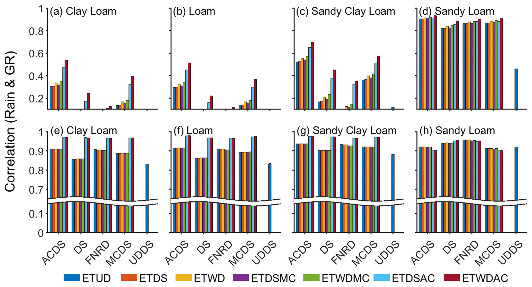
Figure 8Correlation between annual rain and annual GR under the (a–d) Shenmu climate and the (e–h) Beit Dagan climate for (a, e) clay loam, (b, f) loam, (c, g) sandy clay loam, and (d, h) sandy loam. Note that the colors indicate the ET synthesis method.
We find that there are high correlations (correlation coefficient > 0.8) between the annual rain and the annual GR for sandy loam soil under both climate conditions and, except for the UDDS method (correlation coefficient = 0.46), regardless of the rain and ET synthesis methods used (see panels d and h of Fig. 8). This high correlation is expected due to the high infiltration rate, which reduces the actual ET. For the UDDS method, in sandy loam soil, we find that the correlation is smaller for an area with summer rains due to the effect of the high ET during the rainy period.
For the three other soil types, we find a considerably higher correlation under winter rain (panels a–c) than under summer rain conditions (panels e–g). Under winter rain conditions, the correlation is high regardless of the ET and rain synthesis methods used, with a somewhat weaker correlation for the UDDS method for the reasons mentioned above. The strongest correlation is obtained for the annually corrected ETref (for both ETDSAC and ETWDAC). Under summer rain conditions, the ACDS rain synthesis method yields the highest correlation, and FNRD yields the smallest correlation. Under summer rain, UDDS shows a negligible correlation, and the same is true for FNRD with loam and clay loam soil types. Only MCDS and ACDS yield apparent correlations, due to the fact that these methods increase the frequency of large and small rain values.
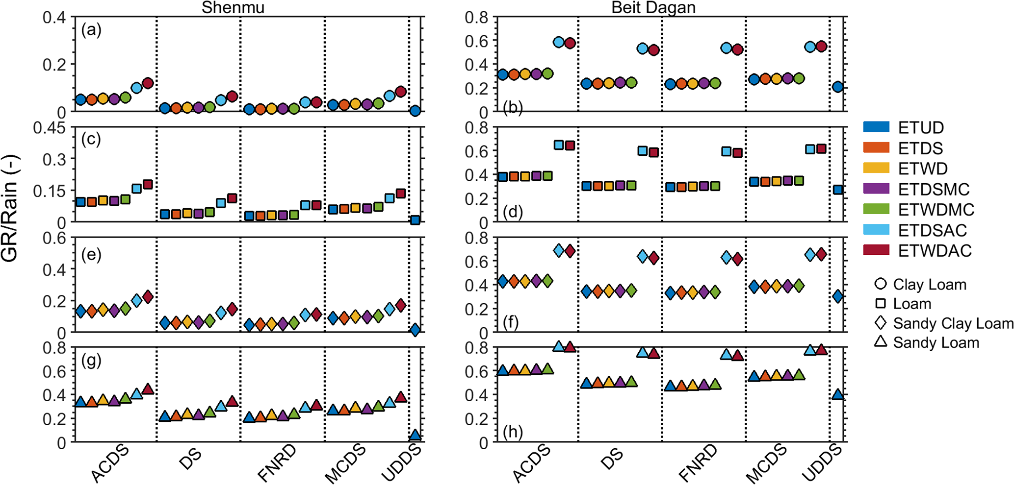
Figure 9The ratio between GR and rain for different climate conditions, rain and ETref synthesis methods, and soil types.
3.5 The ratio between GR and rainfall
The rain and ET synthesis methods affect the rain amount and the actual ET, respectively. Therefore, it is difficult to assess the effect of each method separately. In order to better delineate the role of the methods, we examine the fraction of rain that turns into GR flux. In Fig. 9, we depict the ratio between the accumulated GR flux and the accumulated rainfall. The left panels correspond to Shenmu climate conditions, and the right panels correspond to Beit Dagan conditions. The rows correspond to the different soil types as indicated. In each panel, the ratios are presented for the different combinations of rain and ETref synthesis methods. There is similarity between the estimated GR rain ratio ranges (Fig. 9) and corresponding ratios reported in the literature. Gates et al. (2011) indicated that the GR rain ratio is between 0.11 and 0.18 in the Loess Plateau, similar to our estimates for the finer soil types under Shenmu climate conditions (panels a, c, and e of Fig. 9). For sandy soil, Zhang et al. (2020) reported a GR rain ratio of about 0.58 in the Loess Plateau, slightly above our estimates for sandy loam soil under Shenmu climate conditions (panel g of Fig. 9). Gvirtzman (2002) suggested a recharge coefficient of 0.3 for the entire Israeli coastal aquifer, which is lower than our estimates for the finer soil types under Beit Dagan climate conditions (panels b, d, and f of Fig. 9). For sandy soil types, Eriksson and Khunakasem (1969) and Turkeltaub et al. (2015) showed that the GR fluxes can be higher than 300 mm yr−1, corresponding to a GR rain ratio larger than 0.5.
For winter rain, in Beit Dagan (right column of Fig. 9), we find that the ratio is not very sensitive to the rain synthesis method, with the exception of the UDDS, which results in a lower ratio due to the expected higher actual ET. We also find that the ETDSAC and ETWDAC ETref synthesis methods yield the largest ratio, namely the largest fraction of rain infiltration into the groundwater. This higher ratio is the result of the wider distribution of ETref values, which results in a smaller actual ET (because ETref values above a certain threshold do not increase the actual ET).
For summer rain, the ratio is much smaller due to the larger ET. However, the same dependence on the rain and ETref synthesis methods that is observed for Beit Dagan is also apparent here.
There are different methods that can be used to synthesize the rain and ETref in order to study the dynamics of GR fluxes. The synthesis is often based on measurement records, but only certain aspects of the measured statistics are preserved in the synthesis method. Here, we considered five different methods for rain synthesis and seven methods for ETref synthesis (note that UDDS specifies both the rain and the ETref synthesis method). The different methods are all based on the statistics of the measured daily values for each calendar month. However, preserving the daily statistics alters the monthly and annual statistics, and the methods considered here offer corrections in order to match the mean and variance of the monthly or annual statistics. We find that the statistics of GR fluxes depends on the synthesis method. Namely, the GR fluxes depend on the characteristics of the rain and ETref statistics that were preserved in the synthesis method. For winter rain conditions, the different synthesis methods yield similar GR fluxes and similar ratios between the GR fluxes and the rain amounts. Notably, preserving the annual statistics of ETref yields substantially higher GR fluxes and higher ratios between the GR flux and the rain amount. This effect is due to the broader distribution of ETref values that this method yields. The very large ETref values do not increase the actual ET, while the low values decrease the actual ET, thereby increasing the GR flux. For summer rain conditions, the fraction of rain that infiltrates is smaller than in winter rain conditions due to the increased ET. However, a similar dependence on the synthesis methods is found. An exception to the abovementioned remarks is the GR flux through sandy loam soil, which shows a much weaker sensitivity to the synthesis methods and climate conditions due the fast infiltration rates of surface water in this soil type. The correlations between the annual rain and the GR flux vary with the climate conditions, soil type, and rain and ETref synthesis methods. Therefore, one should be careful when applying measurement-based statistics of rain and ETref to studies of GR fluxes. The most representative synthesis method may be very different for different locations with certain soil types and climate conditions. The methods suggested in this study allow the identification of the most adequate synthesis method for different locations and climate conditions. Moreover, the results provide insights regarding the multiple timescales affecting GR.
The distribution of the annual GR estimated by the monthly corrected DS data, MCDS and ETDSMC, is found to be the closest to the distribution of the annual GR estimated using the observed data. Yet, this conclusion is limited to the two locations considered here and to the simplified model used. Further studies spanning more climate conditions, soil types, and soil water models are required in order to explain and generalize this result.
The code used in this research will be made available upon reasonable request.
The data used in this research will be made available upon reasonable request.
The supplement related to this article is available online at: https://doi.org/10.5194/hess-27-289-2023-supplement.
TT and GB designed the research, analyzed the data, and wrote the manuscript. TT performed the numerical simulations.
The contact author has declared that neither of the authors has any competing interests.
Publisher’s note: Copernicus Publications remains neutral with regard to jurisdictional claims in published maps and institutional affiliations.
We thank the reviewers for providing helpful and constructive feedback.
This paper was edited by Gerrit H. de Rooij and reviewed by Tongchao Nan and one anonymous referee.
Allen, R. G., Pereira, L. S., Raes, D., and Smith, M.: Crop evapotranspiration-Guidelines for computing crop water requirements-FAO Irrigation and drainage paper 56, Fao, Rome, 300, D05109, https://www.fao.org/3/x0490e/x0490e00.htm (last access: 11 January 2023), 1998. a, b, c
Baram, S., Kurtzman, D., and Dahan, O.: Water percolation through a clayey vadose zone, J. Hydrol., 424–425, 165–171, https://doi.org/10.1016/j.jhydrol.2011.12.040, 2012. a
Barron, O. V., Crosbie, R. S., Dawes, W. R., Charles, S. P., Pickett, T., and Donn, M. J.: Climatic controls on diffuse groundwater recharge across Australia, Hydrol. Earth Syst. Sci., 16, 4557–4570, https://doi.org/10.5194/hess-16-4557-2012, 2012. a
Batalha, M. S., Barbosa, M. C., Faybishenko, B., and Van Genuchten, M. T.: Effect of temporal averaging of meteorological data on predictions of groundwater recharge, J. Hydrol. Hydromech., 66, 143–152, https://doi.org/10.1515/johh-2017-0051, 2018. a
Burton, A., Kilsby, C. G., Fowler, H. J., Cowpertwait, P. S., and O'Connell, P. E.: RainSim: A spatial-temporal stochastic rainfall modelling system, Environ. Model. Softw., 23, 1356–1369, https://doi.org/10.1016/j.envsoft.2008.04.003, 2008. a
Cao, G., Scanlon, B. R., Han, D., and Zheng, C.: Impacts of thickening unsaturated zone on groundwater recharge in the North China Plain, J. Hydrol., 537, 260–270, https://doi.org/10.1016/j.jhydrol.2016.03.049, 2016. a
Carsel, R. F. and Parrish, R. S.: Developing joint probability distributions of soil water retention characteristics, Water Resour. Res., 24, 755–769, 1988. a, b
Crosbie, R. S., Scanlon, B. R., Mpelasoka, F. S., Reedy, R. C., Gates, J. B., and Zhang, L.: Potential climate change effects on groundwater recharge in the High Plains Aquifer, USA, Water Resour. Res., 49, 3936–3951, https://doi.org/10.1002/wrcr.20292, 2013. a, b
Cuthbert, M. O., Taylor, R. G., Favreau, G., Todd, M. C., Shamsudduha, M., Villholth, K. G., MacDonald, A. M., Scanlon, B. R., Kotchoni, D. O., Vouillamoz, J. M., Lawson, F. M., Adjomayi, P. A., Kashaigili, J., Seddon, D., Sorensen, J. P., Ebrahim, G. Y., Owor, M., Nyenje, P. M., Nazoumou, Y., Goni, I., Ousmane, B. I., Sibanda, T., Ascott, M. J., Macdonald, D. M., Agyekum, W., Koussoubé, Y., Wanke, H., Kim, H., Wada, Y., Lo, M. H., Oki, T., and Kukuric, N.: Observed controls on resilience of groundwater to climate variability in sub-Saharan Africa, Nature, 572, 230–234, https://doi.org/10.1038/s41586-019-1441-7, 2019. a
Dee, D. P., Uppala, S. M., Simmons, A. J., Berrisford, P., Poli, P., Kobayashi, S., Andrae, U., Balmaseda, M. A., Balsamo, G., Bauer, P., Bechtold, P., Beljaars, A. C. M., van de Berg, I., Biblot, J., Bormann, N., Delsol, C., Dragani, R., Fuentes, M., Greer, A. J., Haimberger, L., Healy, S. B., Hersbach, H., Holm, E. V., Isaksen, L., Kallberg, P., Kohler, M., Matricardi, M., McNally, A. P., Mong-Sanz, B. M., Morcette, J.-J., Park, B.-K., Peubey, C., de Rosnay, P., Tavolato, C., Thepaut, J. N., and Vitart, F.: The ERA-Interim reanalysis: Configuration and performance of the data assimilation system, Q. J. Roy. Meteor. Soc., 137, 553–597, https://doi.org/10.1002/qj.828, 2011. a
Döll, P. and Fiedler, K.: Global-scale modeling of groundwater recharge, Hydrol. Earth Syst. Sci., 12, 863–885, https://doi.org/10.5194/hess-12-863-2008, 2008. a
Eriksson, E. and Khunakasem, V.: Chloride concentration in groundwater, recharge rate and rate of deposition of chloride in the Israel coastal pain, J. Hydrol., 7, 178–197, https://doi.org/10.1016/0022-1694(69)90055-9, 1969. a, b
Fan, Y., Li, H., and Miguez-Macho, G.: Global patterns of groundwater table depth, Science, 339, 940–943, https://doi.org/10.1126/science.1229881, 2013. a
Food and Agricultural Organization (FAO): Map of aridity (Global – ∼ 19 km), Rome, https://data.apps.fao.org/map/catalog/static/api/records/221072ae-2090-48a1-be6f-5a88f061431a last access: 4 January 2023. a, b
Gates, J. B., Scanlon, B. R., Mu, X., and Zhang, L.: Impacts of soil conservation on groundwater recharge in the semi-arid Loess Plateau, China, Hydrogeol. J., 19, 865–875, https://doi.org/10.1007/s10040-011-0716-3, 2011. a, b
Gurdak, J. J., Hanson, R. T., McMahon, P. B., Bruce, B. W., McCray, J. E., Thyne, G. D., and Reedy, R. C.: Climate Variability Controls on Unsaturated Water and Chemical Movement, High Plains Aquifer, USA, Vadose Zone J., 6, 533–547, https://doi.org/10.2136/vzj2006.0087, 2007. a
Gvirtzman, H.: Israel Water Resources, Yad Ben-Zvi Press, Jerusalem, https://scholar.google.co.il/scholar?hl=en&as_sdt=0,5&cluster=15955931416706423166 (last access: 11 January 2023), p. 287, 2002 (in Hebrew). a, b
Harris, I., Jones, P., Osborn, T., and Lister, D.: Updated high-resolution grids of monthly climatic observations – the CRU TS3.10 Dataset, Int. J. Climatol., 34, 623–642, https://doi.org/10.1002/joc.3711, 2014. a, b
Hengl, T., De Jesus, J. M., MacMillan, R. A., Batjes, N. H., Heuvelink, G. B., Ribeiro, E., Samuel-Rosa, A., Kempen, B., Leenaars, J. G., Walsh, M. G., and Gonzalez, M. R.: SoilGrids1km – Global soil information based on automated mapping, PLoS ONE, 9, e105992, https://doi.org/10.1371/journal.pone.0105992, 2014. a, b
Hu, W., Wang, Y., Li, H., Huang, M., Hou, M., Li, Z., She, D., and Si, B.: Dominant role of climate in determining spatio-temporal distribution of potential groundwater recharge at a regional scale, J. Hydrol., 578, 124042, https://doi.org/10.1016/j.jhydrol.2019.124042, 2019. a
Huang, T., Pang, Z., Liu, J., Ma, J., and Gates, J.: Groundwater recharge mechanism in an integrated tableland of the Loess Plateau, northern China: insights from environmental tracers, Hydrogeol. J., 25, 2049–2065, https://doi.org/10.1007/s10040-017-1599-8, 2017. a
Istanbulluoglu, E. and Bras, R. L.: On the dynamics of soil moisture, vegetation, and erosion: Implications of climate variability and change, Water Resour. Res., 42, 1–17, https://doi.org/10.1029/2005WR004113, 2006. a
Kass, A., Gavrieli, I., Yechieli, Y., Vengosh, A., and Starinsky, A.: The impact of freshwater and wastewater irrigation on the chemistry of shallow groundwater: a case study from the Israeli Coastal Aquifer, J. Hydrol., 300, 314–331, https://doi.org/10.1016/j.jhydrol.2004.06.013, 2005. a
Keese, K. E., Scanlon, B. R., and Reedy, R. C.: Assessing controls on diffuse groundwater recharge using unsaturated flow modeling, Water Resour. Res., 41, 1–12, https://doi.org/10.1029/2004WR003841, 2005. a
Kingston, D. G. and Taylor, R. G.: Sources of uncertainty in climate change impacts on river discharge and groundwater in a headwater catchment of the Upper Nile Basin, Uganda, Hydrol. Earth Syst. Sci., 14, 1297–1308, https://doi.org/10.5194/hess-14-1297-2010, 2010. a
Kurtzman, D. and Scanlon, B. R.: Groundwater Recharge through Vertisols: Irrigated Cropland vs. Natural Land, Israel, Vadose Zone J., 10, 662–674, https://doi.org/10.2136/vzj2010.0109, 2011. a
Kurtzman, D., Baram, S., and O., D.: Soil–aquifer phenomena affecting groundwater under vertisols: a review, Hydrology and Earth System Sciences, 20, 1–12, https://doi.org/10.5194/hess-20-1-2016, 2016. a
Lima, C. H., Kwon, H. H., and Kim, Y. T.: A Bernoulli-Gamma hierarchical Bayesian model for daily rainfall forecasts, J. Hydrol., 599, 126317, https://doi.org/10.1016/j.jhydrol.2021.126317, 2021. a
Moeck, C., Grech-Cumbo, N., Podgorski, J., Bretzler, A., Gurdak, J. J., Berg, M., and Schirmer, M.: A global-scale dataset of direct natural groundwater recharge rates: A review of variables, processes and relationships, Sci. Total Environ., 717, 137042, https://doi.org/10.1016/j.scitotenv.2020.137042, 2020. a, b
Mualem, Y.: A New Model for Predicting the Hydraulic Conductivity of Unsaturated Porous Media, Water Resour. Res., 12, 513–522, 1976. a
Nasta, P., Gates, J. B., and Wada, Y.: Impact of climate indicators on continental-scale potential groundwater recharge in Africa, Hydrol. Process., 30, 3420–3433, https://doi.org/10.1002/hyp.10869, 2016. a
Ng, G.-H. C., McLaughlin, D., Entekhabi, D., and Scanlon, B. R.: Probabilistic analysis of the effects of climate change on groundwater recharge, Water Resour. Res., 46, 1–18, https://doi.org/10.1029/2009wr007904, 2010. a
Owor, M., Taylor, R. G., Tindimugaya, C., and Mwesigwa, D.: Rainfall intensity and groundwater recharge: Empirical evidence from the Upper Nile Basin, Environ. Res. Lett., 4, 035009, https://doi.org/10.1088/1748-9326/4/3/035009, 2009. a
Rimon, Y., Nativ, R., and Dahan, O.: Physical and chemical evidence for pore-scale dual-domain flow in the vadose zone, Vadose Zone J., 9, 1–10, https://doi.org/10.2136/vzj2009.0113, 2011. a
Rodriguez-Iturbe, I., Porporato, A., Rldolfi, L., Isham, V., and Cox, D. R.: Probabilistic modelling of water balance at a point: The role of climate, soil and vegetation, P. Roy. Soc. A-Math. Phy., 455, 3789–3805, https://doi.org/10.1098/rspa.1999.0477, 1999. a, b
Rosenberg, N. J., Epstein, D. J., Wang, D., Vail, L., Srinivasan, R., and Arnold, J. G.: Possible impacts of global warming on the hydrology of the Ogallala aquifer region, Climatic Change, 42, 677–692, https://doi.org/10.1023/A:1005424003553, 1999. a
Scanlon, B. R., Stonestrom, D. A., Reedy, R. C., Leaney, F. W., Gates, J., and Cresswell, R. G.: Inventories and mobilization of unsaturated zone sulfate, fluoride, and chloride related to land use change in semiarid regions, southwestern United States and Australia, Water Resour. Res., 45, W00A18, https://doi.org/10.1029/2008WR006963, 2009. a
Šimŭnek, J., Van Genuchten, M. T., and Šejna, M.: The HYDRUS software package for simulating the two-and three-dimensional movement of water, heat, and multiple solutes in variably-saturated porous media, Dep. Environmental Sciences, Univ. Calif., Riverside, CA., version 4.08. HYDRUS Software Series 3, https://www.pc-progress.com/Downloads/Pgm_hydrus1D/HYDRUS1D-4.17.pdf (last access: 4 January 2023), 2009. a
Small, E. E.: Climatic controls on diffuse groundwater recharge in semiarid environments of the southwestern United States, Water Resour. Res., 41, 1–17, https://doi.org/10.1029/2004WR003193, 2005. a, b, c, d, e, f, g, h
Snyder, N. P., Whipple, K. X, Tucker, G. E., and Merritts, D. J.: Importance of a stochastic distribution of floods and erosion thresholds in the bedrock river incision problem, J. Geophys. Res., 108, 2117, https://doi.org/10.1029/2001JB001655, 2003. a, b
Stern, R. D. and Coe, R.: A Model Fitting Analysis of Daily Rainfall Data, J. R. Stat. Soc. A-G., 147, 1–34, https://doi.org/10.2307/2981736, 1984. a
Strobach, E. and Bel, G.: The contribution of internal and model variabilities to the uncertainty in CMIP5 decadal climate predictions, Clim. Dynam., 49, 3221–3235, 2017. a
Tao, Z., Li, H., Neil, E., and Si, B.: Groundwater recharge in hillslopes on the Chinese Loess Plateau, J. Hydrol.-Regional Studies, 36, 100840, https://doi.org/10.1016/j.ejrh.2021.100840, 2021. a
Tencaliec, P., Favre, A. C., Naveau, P., Prieur, C., and Nicolet, G.: Flexible semiparametric generalized Pareto modeling of the entire range of rainfall amount, Environmetrics, 31, 1–20, https://doi.org/10.1002/env.2582, 2020. a, b, c
Turkeltaub, T., Kurtzman, D., Bel, G., and Dahan, O.: Examination of groundwater recharge with a calibrated/validated flow model of the deep vadose zone, J. Hydrol., 522, 618–627, https://doi.org/10.1016/j.jhydrol.2015.01.026, 2015. a, b, c
Turkeltaub, T., Jia, X., Zhu, Y., Shao, M. A., and Binley, A.: Recharge and Nitrate Transport Through the Deep Vadose Zone of the Loess Plateau: A Regional-Scale Model Investigation, Water Resour. Res., 54, 4332–4346, https://doi.org/10.1029/2017WR022190, 2018. a, b
Turkeltaub, T., Ascott, M. J., Gooddy, D. C., Jia, X., Shao, M. A., and Binley, A.: Prediction of regional‐scale groundwater recharge and nitrate storage in the vadose zone: A comparison between a global model and a regional model, Hydrol. Process., 34, 3347–3357, https://doi.org/10.1002/hyp.13834, 2020. a
Uppala, S. M., Kållberg, P. W., Simmons, A. J., Andrae, U., Da Costa Bechtold, V., Fiorino, M., Gibson, J., Haseler, J., Her-nandez, A., Kelly, G. A., Li, X., Onogi, K., Saarinen, S., Sokka, N., Allan, R. P., Anderson, E., Arpe, K., Balmaseda, M. A., Beljaars, A. C. M., Van De Berg, L., Bidlot, J., Bormann, N., Caires, S., Chevallier, F., Dethof, A., Dragosavac, M., Fisher, M., Fuentes, M., Hagemann, S., Hólm, E., Hoskins, B. J., Isaksen, L.and Janssen, P. A. E. M., Jenne, R., Mcnally, A. P., Mahfouf, J.-F., Morcrette, J.-J., Rayner, N. A., Saunders, R. W., Simon, P., Sterl, A., Trenbreth, K. E., Untch, A., Vasiljevic, D., Viterbo, P., and Woollen, J.: The ERA-40 re-analysis, Q. J. Roy. Meteor. Soc., 131, 2961–3012, https://doi.org/10.1256/qj.04.176, 2005. a
van Beek, L. P. H.: Forcing PCR-GLOBWB with CRU data, Tech. Rep., http://vanbeek.geo.uu.nl/suppinfo/vanbeek2008.pdf (last access: 30 June 2022), 2008. a, b
Van Genuchten, M. T.: A closed-form equation for predicting the hydraulic conductivity of unsaturated soils, Soil Sci. Soc. Am. J., 44, 892–898, https://doi.org/10.2136/sssaj1980.03615995004400050002x, 1980. a
Wang, P., Quinlan, P., and Tartakovsky, D. M.: Effects of spatio-temporal variability of precipitation on contaminant migration in the vadose zone, Geophys. Res. Lett., 36, L12404, https://doi.org/10.1029/2009GL038347, 2009. a
Wohling, D. L., Leaney, F. W., and Crosbie, R. S.: Deep drainage estimates using multiple linear regression with percent clay content and rainfall, Hydrol. Earth Syst. Sci., 16, 563–572, https://doi.org/10.5194/hess-16-563-2012, 2012. a, b
Wu, Q., Si, B., He, H., and Wu, P.: Determining Regional-Scale Groundwater Recharge with GRACE and GLDAS, Remote Sensing, 11, 1–22, https://doi.org/10.3390/rs11020154, 2019. a
Zhang, Z., Wang, W., Gong, C., and Zhang, M.: A comparison of methods to estimate groundwater recharge from bare soil based on data observed by a large-scale lysimeter, Hydrol. Process., 34, 2987–2999, https://doi.org/10.1002/hyp.13769, 2020. a