Application of an improved distributed hydrological model based on the soil–gravel structure in the Niyang River basin, Qinghai–Tibet Plateau

Runoff formation and hydrologic regulation mechanisms in mountainous cold regions are the basis for investigating the response patterns of hydrological processes under climate change. Because of plate movements and climatic effects, the surface soils of bare lands and grasslands on the Qinghai–Tibet Plateau (QTP) are thin, and the soil below the surface contains abundant gravel. This characteristic geological structure, combined with snow and frozen soil, affects the water cycle in this region. To investigate the influence of the underlying surface structure on water–heat transport and water circulation processes on the QTP, a comprehensive study was performed combining water–heat transfer field experiments, and a water and energy transfer process model for the QTP (WEP-QTP) was developed based on the original water and energy transfer process model in cold regions (WEP-COR). The Niyang River basin, located on the QTP, was selected as the study area to evaluate the consistency between theoretical hypotheses, observations, and modeling results. The model divided the uniform soil profile into a dualistic soil–gravel structure. When no phase change was present in the ground, two infiltration models based on the dualistic soil–gravel structure were developed; these used the Richards equation to model a non-heavy rain scenario and the multilayer Green–Ampt model for a heavy rain scenario. During the freeze–thaw period, a water–heat coupling model based on the snow–soil–gravel layer structure was constructed. By considering gravel, the improved model corrected the overestimation of the moisture content below the surface soil predicted by the original model and reduced the moisture content relative error (RE) from 33.74 % to −12.11 %. The addition of the snow layer not only reduced the temperature fluctuation of the surface soil, but also revised the overestimation of the freeze–thaw speed predicted by the original model with the help of the gravel. The temperature root-mean-square error was reduced from 1.16 to 0.86 ^∘C. In the fully thawed period, the dualistic soil–gravel structure improved the regulation effect of groundwater on flow, thus stabilizing the flow process. The maximum RE at the flow peak and trough decreased by 88.2 % and 21.3 %, respectively. In the freeze–thaw period, by considering the effect of the snow–soil–gravel layer structure, the freezing and thawing processes of WEP-QTP lagged behind those of WEP-COR by approximately 1 month. The groundwater simulated by WEP-QTP had more time to recharge the river, which better represented the observed “tailing” process from September onwards. The flow simulated by the WEP-QTP model was more accurate and closer to the actual measurements, with Nash–Sutcliffe efficiency > 0.75 and |RE| < 10 %. The improved model reflects the effects of the typical QTP environment on water–heat transport and water cycling and can thus be used for hydrological simulation on the QTP.

1 Introduction

The Qinghai–Tibet Plateau (QTP), also known as the “Asian water tower,” is a major cold mountainous area located at low latitude and high altitude. This region has characteristic geology and landforms, is sensitive to climate change (Liu et al., 2019), and is vital for the water resource security of China and Southeast Asia (Liu et al., 2020). The extensive glaciers, snow cover, and permanently and seasonally frozen soil in the area have major impacts on the water cycle (Li et al., 2016; Ding et al., 2020). Unraveling the mechanisms of runoff formation and hydrological regulation in this region is the basis for studying the response patterns of hydrological processes under a changing climate.

In both permafrost and permafrost-free areas, the ground undergoes seasonal freezing and thawing, which has received a lot of attention regarding hydrological research because of the great variety of biological and physical processes occurring on the surface and subsurface (Chen et al., 2014; Kurylyk et al., 2014). During soil freezing, ice in the seasonally thawed layer blocks most of the pores in the soil, hinders infiltration, and thus affects water movement in the soil (Cheng and Jin, 2013). In terms of the hydrological cycle, the frozen soil layer prevents rainfall and snowmelt infiltration, forcing surface runoff downslope, which may lead to severe flash floods. In addition, frozen soil affects the quantity of groundwater recharge supplemented by infiltration and the distribution ratio of water resources allocated between rivers and lakes (Ireson et al., 2013; Larsbo et al., 2019). The simulation accuracy of water and heat transport in the seasonally thawed layer directly affects the evaluation of water resources and analysis of runoff evolution in the QTP area. However, soil water and heat transfer processes are relatively complex and influenced by several factors (Watanabe and Kugisaki, 2017), such as soil structure (Dai et al., 2019; Franzluebbers, 2002) and heat conduction under snow cover (Lundberg et al., 2016).

As a result of the collision of the Indian and Eurasian plates, there are many gravel and rock fragments within QTP Quaternary sediments (Chen et al., 2015; Deng et al., 2019). The abundance of gravel allows the formation of many interconnected pore channels within these sediments, thus increasing their saturated hydraulic conductivity (Beibei et al., 2009). The greater thermal conductivity and heat capacity of gravel compared to those of dry soil also affect the heat transfer process (Yi et al., 2013). In addition, due to environmental constraints, physical weathering dominates the soil formation process on the QTP, resulting in a low level of soil mineral decomposition and slow soil development. Although the QTP has a variety of landscapes and surface processes, the grasslands occupy the largest proportion of the land, followed by bare land, the sum of which exceeds 80 % (Zhang and Zhou, 2021). In these areas, the decomposition of biomass occurs mostly in the surface layers of Quaternary sediments because of the low temperatures, resulting in the formation of a thin soil layer that is highly developed and accumulates more organic matter than deeper layers (Sun, 1996). This soil stratification is widespread on the QTP (Yang et al., 2009; Pan et al., 2017). The topsoil (typically 0–20 cm) in these areas is generally a sandy loam with a mixture of sand and gravel below it (Chen et al., 2015).

Many hydrological models have been applied to the QTP, including those developed specifically for water cycle processes in cold regions, such as the Cold Regions Hydrological Model (CRHM) (Zhou et al., 2014), Water balance Simulation Mode (WaSiM) (Sun et al., 2020), Geography and Topography model (GEOtop) (Pan et al., 2016), and Distributed Water-Heat Coupled model (DWHC) (Chen et al., 2018). As these models were constructed for cold regions from the outset, modeling soil freeze–thaw processes and accumulation and melting processes of snow and glaciers is detailed and based on physical mechanisms. However, these models require more input parameters and are generally suitable for small catchments. Some models are improved for the characteristics of cold regions based on non-cold hydrological models, such as the improved Soil and Water Assessment Tool model (SWAT) (Sun et al., 2013), the Variable Infiltration Capacity model (VIC) (Cuo et al., 2015), the Hydrologiska Byråns Vattenbalansavdelning model (HBV) (Bergström et al., 2015), the Water and Energy Budget-based Distributed Hydrological Model (WEB-DHM) (Wang et al., 2010), and the Geomorphology-Based Eco-Hydrological Model (GBEHM) (Gao et al., 2018). These models exhibited improved performance in cold regions by using heat transfer models or temperature-index models to simulate the freeze–thaw process of soil and the melting process of snow (Ala-Aho et al., 2021; Gao et al., 2021). A few studies have also coupled soil freeze–thaw processes or accumulation and melting processes of snow and glaciers with conceptual hydrological models, such as the semi-distributed conceptual frozen soil hydrological model (FLEX-Topo-FS) (Gao et al., 2022) and the distributed conceptual model involving snow and glacier modules (FLEXD-SG) (Gao et al., 2020), based on the perceptual model and a topography-driven modelling approach (FLEX-Topo) (Savenije, 2010), the flexible modeling framework of which can improve the performance of the model in information-poor cold regions while avoiding over-parameterization. However, these models above generally define the simulated object of the water–heat coupled transport process as a homogeneous medium and ignore the stratified soil structure when applied to the QTP. Further, the effect of gravel on water and heat transfer can be hidden to some extent by calibrating certain parameters. The bias in the simulation of interlayer water and heat transport due to the differences in the hydrodynamic and thermodynamic properties between soil and gravel remain, making it difficult for these models to objectively reflect the hydrological cycle processes under geologically stratified structural conditions in the QTP.

It is particularly important to consider the influence of the unique underlying surface of the QTP on water–heat transport and water circulation, especially in the context of global climate change and frozen soil degradation. The objectives of the present study were to (1) develop infiltration models based on the dualistic soil–gravel structure under fully thawed conditions, (2) develop a modeling framework representing coupled water and heat transfer in the ground based on the snow–soil–gravel layer structure through field water and heat monitoring experiments during the freeze–thaw period (when the temperature of the calculation unit was lower than 0 ^∘C), and (3) investigate the effect of the dualistic soil–gravel structure on the hydrological cycle by building a water and energy transfer process model of the QTP (WEP-QTP) for the Niyang River basin, a tributary of the Yarlung Zangbo River on the QTP.

2 Materials and methods

2.1 Study sites and data

2.1.1 Study area

The Niyang River is located on the left bank of the lower reaches of the Yarlung Zangbo River, between 29^∘28^′–30^∘38^′ N and 92^∘10^′–94^∘35^′ E in the Linzhi area of southeastern Tibet. It originates from Cuomoliang Mountain on the western side of Mila Mountain in the Tibet Autonomous Region of China at an altitude of approximately 5000 m above sea level ($\mathrm{a}.\mathrm{s}.\mathrm{l}.$). The Niyang River flows from west to east through Gongbujiangda County and the town of Bayi and finally flows into the Yarlung Zangbo River in the Bayi District of Nyingchi; it has a vertical drop of 2080 m with an average slope of 0.73 %. The basin is approximately 230 km long from east to west and 110 km wide from north to south. The area of the watershed is 17 535 km², ranking fourth among the five tributaries of the Yarlung Zangbo River, and its runoff is second only to that of the Palungzangbu River. The Niyang River basin is located at the intersection of the east–west and north–south mountain ranges of Tibet. The basin sediments consist of greywacke and litharenite with low to moderate textural and mineralogical maturity (Huyan et al., 2022). The terrain in the watershed is complex, with staggered large and small mountains and large elevation fluctuations. The elevation of the river valley is generally 3000–4000 $\mathrm{m}\mathrm{a}.\mathrm{s}.\mathrm{l}.$ The elevation of most mountain peaks on both sides of the valley is approximately 5000 $\mathrm{m}\mathrm{a}.\mathrm{s}.\mathrm{l}.$, reaching a maximum of 6870 $\mathrm{m}\mathrm{a}.\mathrm{s}.\mathrm{l}.$ The Niyang River basin belongs to the plateau temperate monsoon climate zone. The multiyear average precipitation is affected by the Indian Ocean tropical ocean monsoon. Under the effect of the Indian low pressure, the southwestern monsoon pushes a large quantity of warm and humid air from the Bay of Bengal along the Yarlung Zangbo River valley to the Niyang River basin, causing precipitation in the basin; rainfall is often heavy and varies markedly with elevation. The average elevation of the basin is 4688.6 $\mathrm{m}\mathrm{a}.\mathrm{s}.\mathrm{l}.$, the average annual precipitation is 1416 mm, and the average annual temperature is approximately 8 ^∘C. Evident temperature changes occur from east to west with changing elevation. The frozen soil in the study area is mainly seasonal. Permafrost accounts for approximately 24 % of the basin area, mainly distributed in the upper reaches of the basin and high-altitude areas on both sides of the main stream.

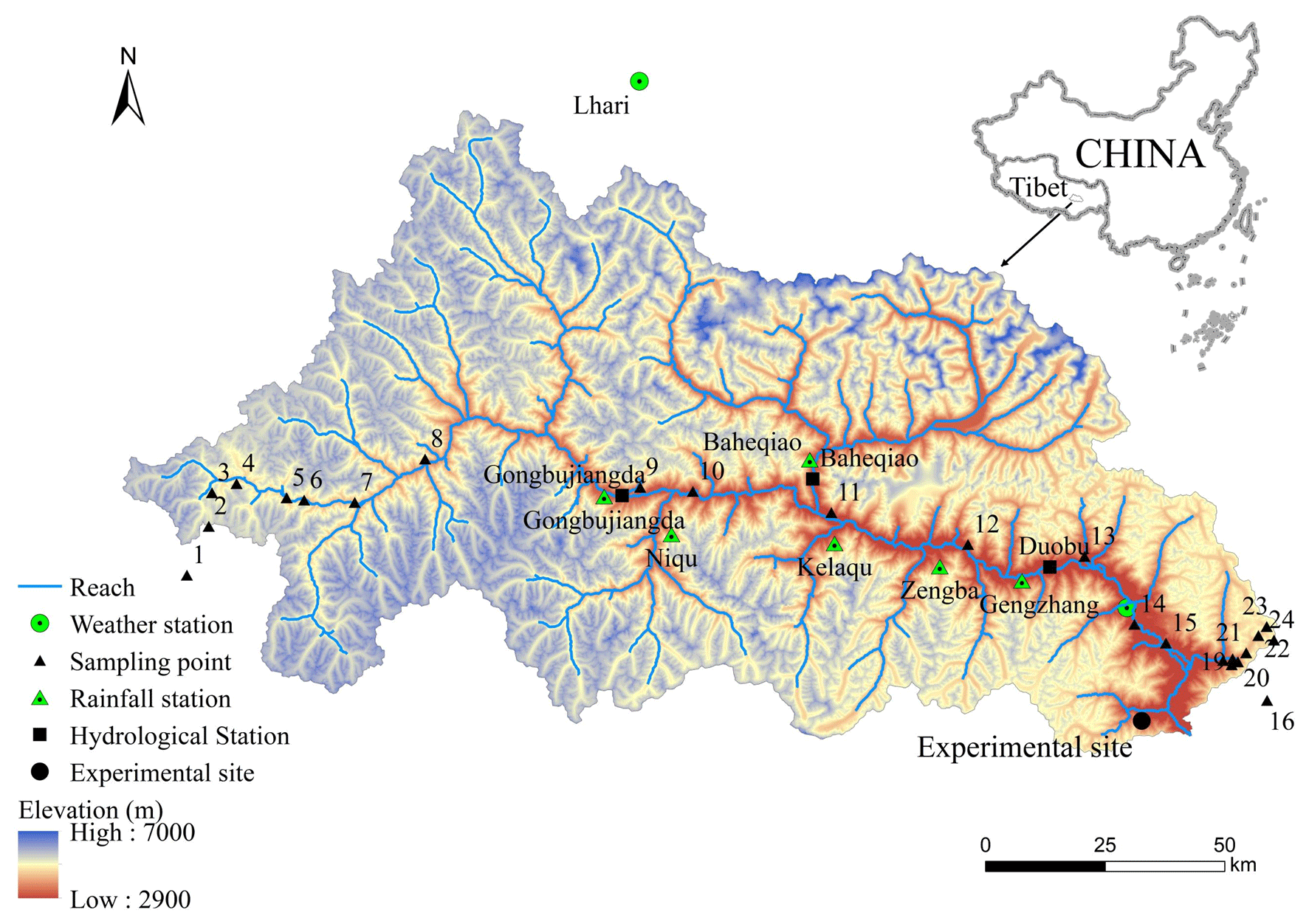
Figure 1 Overview of the Niyang River basin, including the distribution of stations, sampling points, and the experimental site.

In the present study, a water–heat coupling process monitoring experiment was carried out during the freeze–thaw period on the side of Sejila Mountain on the lower reaches of the Niyang River basin. The latitude and longitude of the study site are 29^∘27^′12^′′ N and 94^∘21^′45^′′ E, respectively, and the altitude is 4607 $\mathrm{m}\mathrm{a}.\mathrm{s}.\mathrm{l}.$ The annual average temperature of the experimental site, a seasonally frozen soil area, is 5.28 ^∘C. The experimental period was from 2016 to 2017, during which the freeze–thaw period occurred from November 2016 to March 2017. The distribution of stations within the watershed and location of the experimental area is shown in Fig. 1. Before the field experiment, nuclear magnetic resonance was used to calibrate the water and heat transport monitoring instruments under seasonal freezing and thawing soil conditions on the plateau. A working area with a length of 1.0 m, width of 1.0 m, and depth of 2.0 m was excavated at the experimental site. A time-domain reflectometry sensor was used to monitor the liquid water content, a PT100 sensor was used to measure the temperature, and a TensionMark sensor was used to measure the soil water potential; each was installed every 10 cm vertically in the experimental pit to a depth of 1.6 m. Following installation, the pit was backfilled with undisturbed soil, and data were collected automatically. During the experiment, the monitoring instrument was inspected regularly, and the snow thickness was measured at the same time.

2.1.2 Data description

The data required for this study were mainly divided into two categories: (1) data required for model construction (including meteorology, geology and landforms, terrain, soil type, land-use type, vegetation index, and glacier data); and (2) data used to verify the model results (including historical and experimental monitoring data).

Meteorological data, including temperature, relative humidity, sunshine hours, and wind speed, were collected by the Nyingchi Meteorological Station within the basin and the Jiali Meteorological Station outside the basin from 1961 to 2018. These data were obtained from the China Meteorological Data Network (http://data.cma.cn, last access: 20 October 2021). In addition to the two meteorological stations, the rainfall data sources also included six rainfall stations (Gongbujiangda, Gengzhang, Baheqiao, Niqu, Kelaqu, and Zengba; data from 2013 to 2015) from the watershed and the contour map of annual precipitation in the Tibet Water Resources Bulletin (2012–2017). The temperature, precipitation, relative humidity, sunshine duration, and wind speed in the basin were interpolated from the meteorological station data using the reversed-distance-squared method. Temperature and precipitation were additionally corrected for elevation. The temperature correction factor was −6 ${}^{\circ }\mathrm{C}{\mathrm{km}}^{-\mathrm{1}}$. For the precipitation data, the precipitation–elevation relationship was determined according to the contour map of annual precipitation in the Tibet Water Resources Bulletin and the precipitation station data. Subsequently, the daily precipitation data were obtained for the basin through elevation interpolation (Wang et al., 2017) of the precipitation data from six rainfall stations and two meteorological stations to avoid precipitation errors at high altitudes caused by altitude limitations of precipitation stations.

Geology and landform data: owing to plate movements and climatic effects, the surface soils of bare land and grassland on the QTP are thin, and the underlying soils contain abundant gravel (Fig. 2). According to the geological characteristics of the QTP, we selected 24 sampling points at different altitudes, from the source to the estuary of the Niyang River basin, for field investigation of soil texture (Fig. 1). Among these, points 1–16 were located along the river, while points 17–24 were distributed from the foot of the mountain to the peak. The soil thicknesses and compositions at the 24 sampling points were measured and analyzed. The surface soil of the Niyang River basin was mainly sandy loam, with average sand, silt, and clay contents of 55.89 %, 31.2 %, and 12.91 %, respectively. The underlying mixture of soil and gravel mainly comprised rounded gravel containing pebbles. The gravel content was approximately 50 %–65 %, while the clay content was 5 %–10 %, and pores were filled with medium- and fine-grained sand. The thickness of the surface soil gradually decreased from the foot to the peak of the mountain; it was greater than 100 cm in the valley and decreased with higher altitude to approximately 40 cm on the upper hillside.

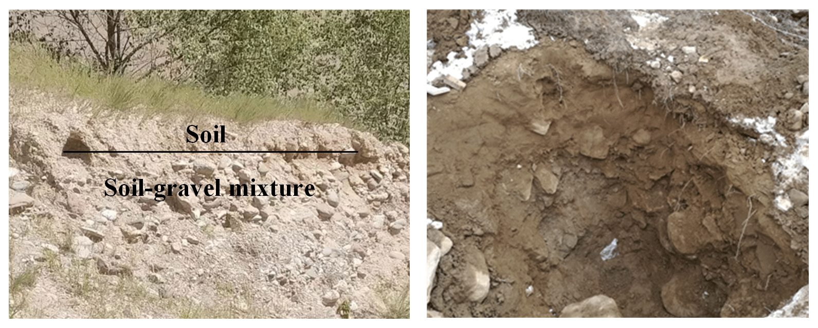
Figure 2 Soil and gravel structure of the Niyang River basin (pictures taken near the experimental site labeled in Fig. 1).

Terrain data: elevation data (digital elevation model, DEM) used in this study were obtained from the SRTM90 (Shuttle Radar Topography Mission), jointly measured by the National Aeronautics and Space Administration and the National Imagery and Mapping Agency with an accuracy of 90 m.

Soil data: soil-type data were obtained from the Chinese Soil Records (http://vdb3.soil.csdb.cn/extend/jsp/introduction, last access: 20 October 2021). Land-use data were obtained from the Resource Environment Science and Database Center, Institute of Geographic Sciences and Natural Resources Research, Chinese Academy of Sciences (http://www.resdc.cn, last access: 20 October 2021); the data resolution was 30 m.

Vegetation index: Moderate Resolution Imaging Spectroradiometer data (https://ladsweb.modaps.eosdis.nasa.gov/search/, last access: 20 October 2021) from 2000 to 2017 were selected as the data source. Among these data, the leaf area index accuracy was 500 m and the normalized difference vegetation index accuracy was 250 m; these were mainly used to calculate evaporation and vegetation interception processes, respectively.

Glacier data: the glacier data included the second glacial catalog dataset of China (1:100 000) and Landsat Thematic Mapper (TM)/Enhanced Thematic Mapper Plus (ETM+)/Operational Land Imager (OLI)/Environment for Visualizing Images (ENVI) remote-sensing images. The second glacier inventory data were obtained from the China National Cryosphere Desert Data Center (http://www.ncdc.ac.cn/portal/metadata, last access: 20 October 2021). Landsat data were obtained from the data-sharing platform of the United States Geological Survey (http://glovis.usgs.gov/, last access: 20 October 2021). ENVI software was used to extract glaciers, and the boundaries of the glaciers were finally determined with reference to Google Earth imagery. The glaciers in the basin were classified according to China's second glacier-cataloging rules, and the glacier area was calculated. The volume of each glacier was calculated using the area–volume empirical formula (Grinsted, 2013; Radić and Hock, 2010).

The distribution of the main hydrologically relevant features of the basin used in the model construction is shown in Appendix A. Model verification data included historical and experimental monitoring data. Historical data included daily measured flow data from the Gongbujiangda Hydrological Station (2013–2016, 2018), Baheqiao Hydrological Station (2013–2014), and Duobu Station (2013–2018). Experimental monitoring data included the snow thickness, soil temperature, and volumetric water content of the experimental site from 2016 to 2017.

2.2 Model improvement

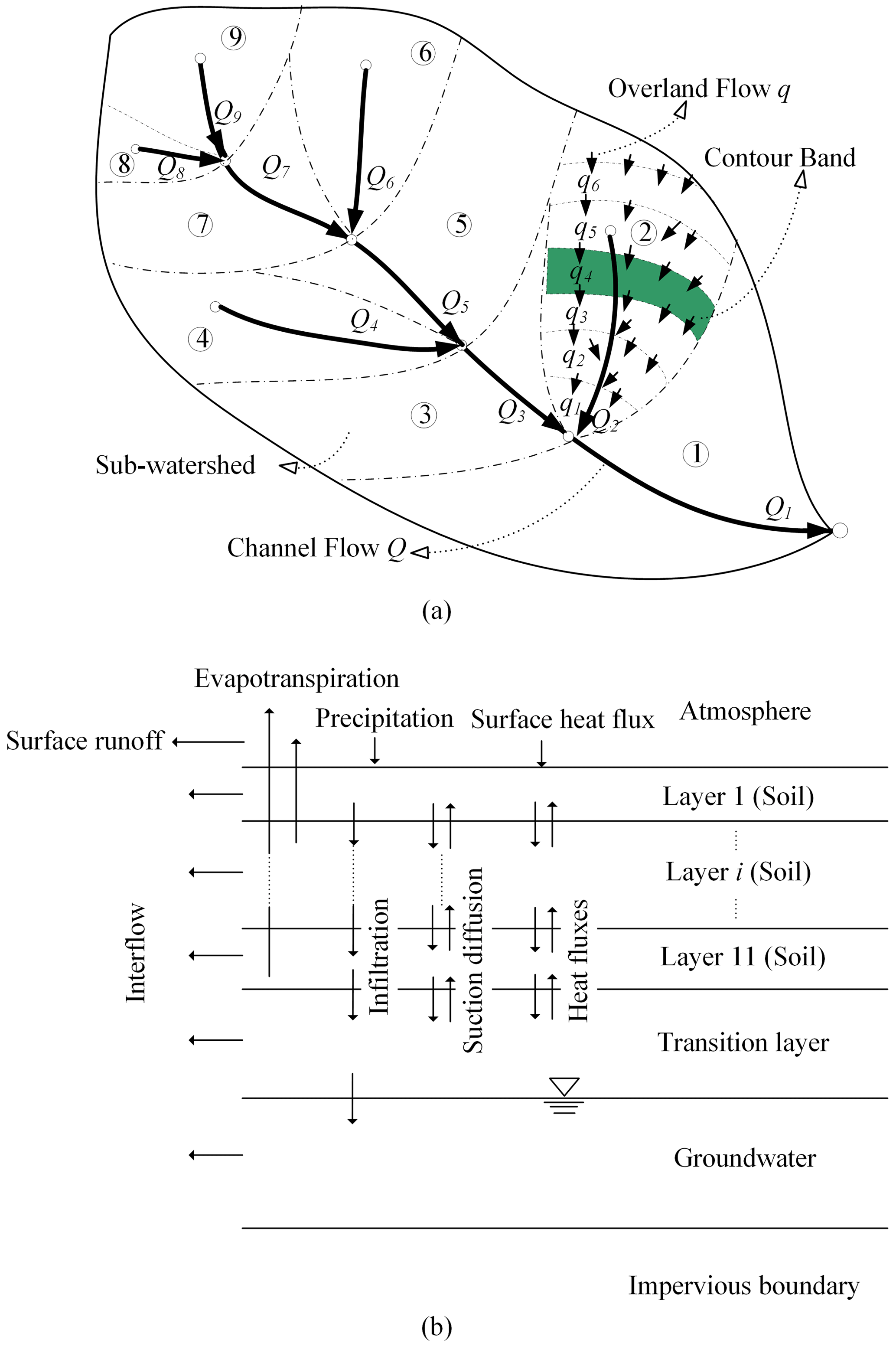
Based on the water and energy transfer processes in cold regions (WEP-COR) model (Li et al., 2019), this study developed the improved WEP-QTP model. The WEP-COR model is a distributed hydrological model. To consider the impact of the topography and land cover on the water cycle in large basins, contour bands were selected as the calculation unit of the WEP-COR model (i.e., bands at different elevation intervals) inside small subbasins. Each unit is classified into five classes: water body, soil–vegetation, irrigated farmland, non-irrigated farmland, and impervious area. The water body class includes rivers, lakes, and glaciers. The soil–vegetation class includes bare land, grassland, and woodland. The impervious area class consists of urban buildings and impervious surfaces. The calculation result of the water and heat flux in each class is weighted by area to obtain the water and heat flux of the contour band. An introduction to the WEP-COR model structure and simulation method is provided in Appendix B.

In contrast to the cold areas where the WEP-COR model is generally applied, the seasonally thawed layer above the impervious boundary (in permafrost regions, the impervious boundary is the permafrost layer) on the QTP is mostly a dualistic soil–gravel structure, which is the key link between surface water and groundwater. Therefore, we took the seasonally thawed layer above the impermeable boundary as the research object and improved the water and heat simulation methods for the fully thawed and freeze–thaw periods in soil–vegetation, irrigated farmland, and non-irrigated farmland areas.

Figure 3 Layers of the dualistic soil–gravel structure (a) and its cross section (b).

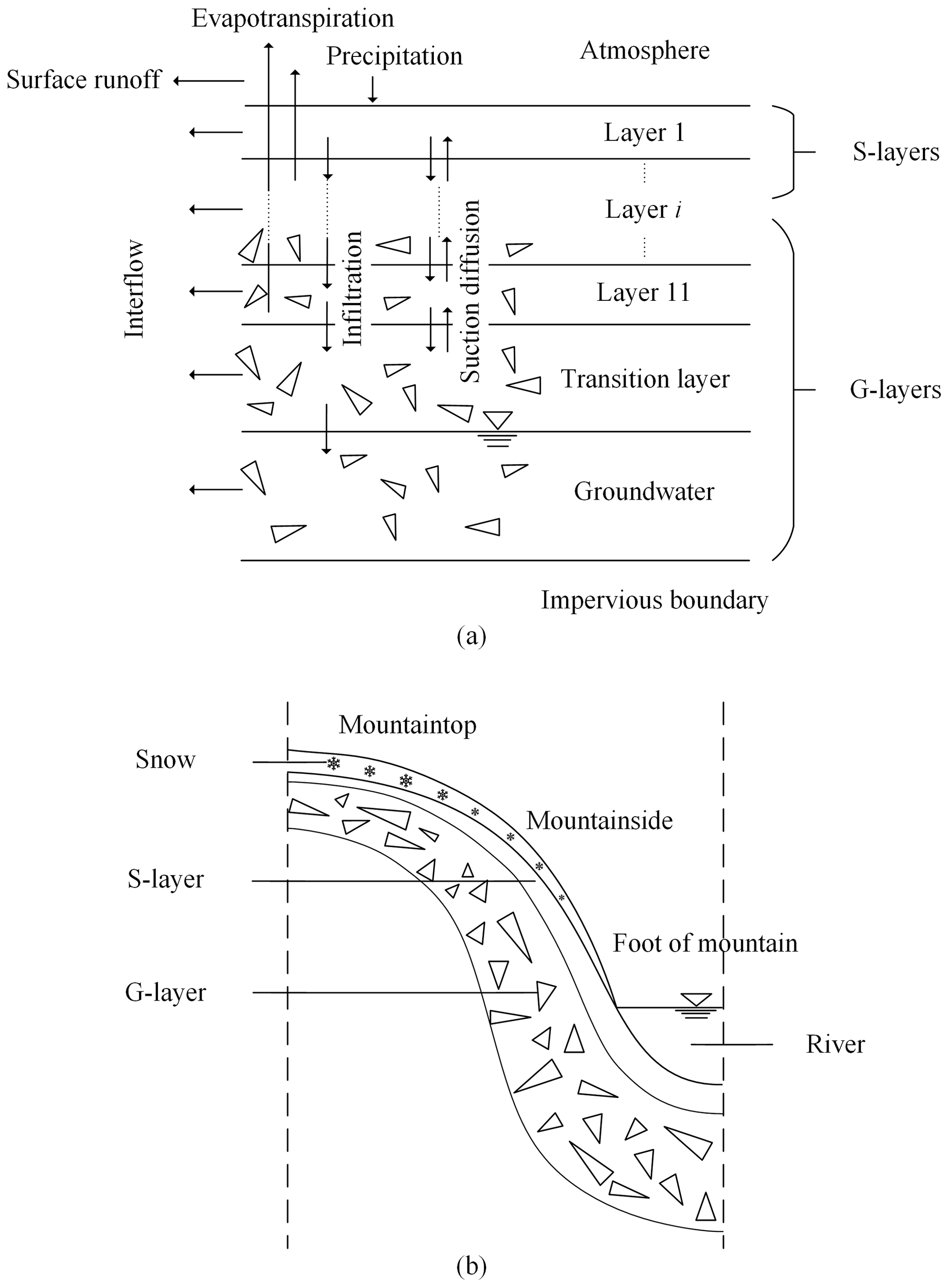
Under fully thawed conditions, the calculation object of water movement was defined as the dualistic soil–gravel structure (Fig. 3a). The upper layers were soil (“s-layers”), whose thickness was determined by the location of the calculation unit and which gradually decreased from the foot to the peak of the mountain (Fig. 3b). The lower layers were a mixture of gravel and soil (“g-layers”), dominated by gravel, the thickness of which was the total thickness of the aquifer and vadose zone above the impermeable boundary minus the surface soil thickness.

During the freeze–thaw period, in addition to considering the impact of gravel on water–heat transfer, the contribution of snow to thermal insulation was also considered. A snow layer was added on top of the dualistic soil–gravel structure. The water–heat coupling simulation object was defined as the snow–soil–gravel layer structure (Fig. 4).

Figure 4 Layers of the snow–soil–gravel layer structure.

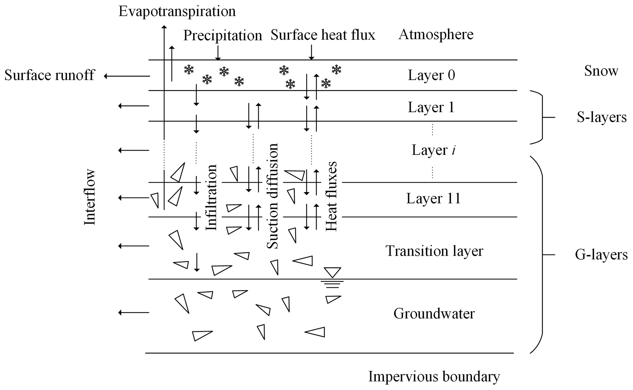
Snow was treated as a single layer (layer 0) in the model, and its thickness was determined by the snow water equivalent and snow density. As the surface soil is more sensitive to changes in atmospheric temperature, the thicknesses of layers 1 and 2 were each set to 10 cm, while the thicknesses of the other s-layers and g-layers were set to 20 cm. Considering the active range of seasonally frozen soil, the depth of the water–heat numerical simulation in the model was set to 2 m. When the depth of groundwater is < 2 m, the depth of the water–heat numerical simulation equates to the depth of groundwater, and when the depth of groundwater is > 2 m, the part below 2 m is treated as the transition layer. The lower boundary was the impermeable layer, and the depth from the surface to the impermeable layer was an adjustable parameter in the model that can be adjusted based on the actual basin conditions. In regions with seasonally frozen soil, the model considered the entire freezing and bidirectional thawing processes of the soil. For the permafrost regions, the surface-layer freezing and thawing processes were considered, while the lower permafrost layer was used as the lower-boundary condition.

2.2.1 Fully thawed period

In the non-heavy rain infiltration scenario, the basic equation describing water movement remained the same and is Darcy's law. However, the high gravel percentage of the g-layer changes its water retention curves and affects its matrix suction under different moisture conditions (Cousin et al., 2003). Therefore, a revised formula for water retention properties of the soil–gravel mixture was used to describe the water retention curves of the lower g-layers (Wang et al., 2013):

$$\begin{array}{}\text{(1)}& {\displaystyle \frac{{\mathit{\theta }}_l-{\mathit{\theta }}_{\mathrm{r}}}{{\mathit{\theta }}_{\mathrm{s}}-{\mathit{\theta }}_{\mathrm{r}}}}=A_{\mathrm{m}}{h}^{-\mathit{\lambda }}(\mathrm{1}-B_{\mathrm{m}}{\mathit{\omega }}_{\text{gravel}}),\end{array}$$

where A_m and B_m are empirical parameters, h is the matrix suction (cm), λ is the pore-size distribution parameter (λ < 1), and ω_gravel is the volume ratio of gravel in the g-layer. Wang et al. (2013) provided a full description of the factors and parameters used in Eq. (1) (A_m = 1.45, B_m = 0.2, λ = 0.18) in this study.

Figure 5 Cumulative infiltration process of the WEP-QTP model.

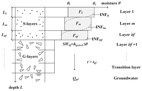
In the heavy-rain infiltration scenario, the multilayer Green–Ampt equation (Jia and Tamai, 1998) was used to calculate the infiltration process when the infiltration front (INF) was in the s-layer, which is the same as in WEP-COR (Eqs. B4 to B11 in Appendix B). As the INF moves to the interface of the s-layer and the g-layer (layer itf), the front movement slows down because the water suction of the g-layer is less than that of the s-layer. When the water has the same potential energy in the s-layer and the g-layer, the INF breaks through the critical surface, and then the infiltration rate stabilizes (Fig. 5). Therefore, a new infiltration model was proposed by improving the method of infiltration rate in the multilayer Green–Ampt equation (Eq. B4 in Appendix B). The stable infiltration rate after the INF breaks through layer itf was calculated as follows:

$$\begin{array}{}\text{(2)}& f_{\text{gravel}}=k_{\text{soil}}\left(\mathrm{1}+{\displaystyle \frac{A_{\text{itf}}}{B_{\text{itf}}+F_{\text{itf}}}}\right),\end{array}$$

where f_gravel is the stable infiltration rate after breaking through layer itf, k_soil is the saturated hydraulic conductivity of the s-layer (mm h⁻¹), F_itf is the cumulative infiltration when the front breaks through layer itf (mm), A_itf is the total water capacity of the s-layers above the interface (mm), and B_itf is the error caused by the different soil moisture content of the s-layers above the interface (mm). A full description of the two parameters A_itf and B_itf has been provided by Jia and Tamai (1998), and their calculation is shown in Appendix B by Eqs. (B5) and (B6).

The gravel increases the porosity in the g-layers, and the pores connect to form a fast channel for transporting water during heavy rain. After the INF breaks through the interface, the infiltrating water preferentially recharges the groundwater through macropores. The accumulated infiltration quantity is calculated as follows:

$$\begin{array}{}\text{(3)}& F=F_{\text{itf}}+Q_{\text{gd}},\end{array}$$

where Q_gd is the quantity of groundwater recharged by infiltration, $Q_{\text{gd}}=f_{\text{gravel}}(t-t_{\text{itf}})$, and t_itf is the time when the INF breaks through the interface.

Under fully thawed conditions, all the water is in a liquid state, and heat conduction has only a minor effect on the water migration process. Therefore, for simulation efficiency, only moisture simulation was performed during this period.

2.2.2 Freeze–thaw period

During the freeze–thaw period, the water–heat coupling simulation object was defined as the snow–soil–gravel layer structure (Fig. 4). On the QTP, variations in temperature and precipitation caused by altitude differences result in more snow accumulation and less melting at higher altitudes. Therefore, avalanches are common in steep/mountainous regions. In this model, a snow thickness threshold was established. When the difference in snow thickness between two adjacent calculation units (the contour bands) exceeds this threshold, an avalanche will occur. The snow in the higher-altitude calculation unit slides into the next unit until the two units have the same snow thickness. The daily variation of snow water equivalent was calculated as follows:

$$\begin{array}{}\text{(4)}& S=S_{\mathrm{p}}-S_{\mathrm{d}}-S_{\mathrm{m}},\end{array}$$

where S is the daily variation of snow water equivalent (mm d⁻¹), S_p is the snow water equivalent from precipitation (mm d⁻¹), S_p is equal to the daily precipitation when the average atmospheric temperature of the day is < 2 ^∘C and S_p = 0 otherwise, S_d is the snow water equivalent variation due to avalanches (mm d⁻¹), and S_m is the quantity of the snowmelt equivalent (mm d⁻¹) calculated using the degree-day factor method (Hock, 1999) as follows:

$$\begin{array}{}\text{(5)}& S_{\mathrm{m}}=d_{\mathrm{f}}(T_{\mathrm{a}}-T_{\mathrm{S}}),\end{array}$$

where d_f is the degree-day factor ($\mathrm{mm}({}^{\circ }\mathrm{C}\mathrm{d}{)}^{-\mathrm{1}}$), T_a is the atmospheric temperature (^∘C), and T_S is the critical temperature of snow melting (^∘C), assuming snow melting begins when T_a > T_S. S_m was treated as precipitation in the model.

The simulation method of water transport under the snow layer was the same as that in the fully thawed period. However, the saturated hydraulic conductivity (K_s) was corrected by temperature and calculated as follows (Chen et al., 2008; Jansson and Karlberg, 2004):

$$\begin{array}{}\text{(6)}& K_{\mathrm{s}}=\left\{\begin{array}{ll}K& T>\mathrm{0},\\ K(\mathrm{0.54}+\mathrm{0.023}T)& T_{\mathrm{f}}\le T\le \mathrm{0},\\ K_{\mathrm{0}}& T<T_{\mathrm{f}},\end{array}\right.\end{array}$$

where K is the initial saturated hydraulic conductivity (cm s⁻¹) and K₀ is the minimum hydraulic conductivity (cm s⁻¹) under freezing conditions. Considering the difference in the hydrodynamic properties of the s-layer and the g-layer, the K₀ value for the s-layer was 0 cm s⁻¹. For the g-layer, owing to the larger pores, K₀ has a value > 0 cm s⁻¹. T is the temperature of the s-layer or the g-layer (^∘C), while T_f is the critical temperature (^∘C) corresponding to the minimum hydraulic conductivity.

Due to the zonal variability in altitude, land surface features, and vegetation characteristics, spatial differences exist in meteorological elements and aerodynamic parameters on the QTP. The use of the energy balance method, which involves multiple meteorological elements and aerodynamic parameters to calculate the heat flux of each contour band, can lead to extensive calculations and an unstable solution process. Therefore, we assumed that the upper boundary of the heat transfer system is the atmosphere, which controls the input and output of energy in the system. The temperature difference between the atmosphere and the surface is the only source of heat conduction. In the presence of snow on the surface, the atmosphere first exchanges energy with the snow, and then the snow exchanges energy with the soil, while in the absence of snow, the atmosphere exchanges energy directly with the soil. The heat transferred to the underlying surface can be calculated from the climate forcing using the following equation (Hu and Islam, 1995):

$$\begin{array}{}\text{(7)}& C_{\text{Vu}}\mathit{\delta }{\displaystyle \frac{\mathrm{d}{T}_{\mathrm{u}}}{\mathrm{d}t}}=G(\mathrm{0},t)-G\left(\mathit{\delta }t\right),\end{array}$$

where C_Vu is the volumetric heat capacity of the underlying surface ($\mathrm{MJ}{\mathrm{m}}^{-\mathrm{3}}{}^{\circ }{\mathrm{C}}^{-\mathrm{1}}$), T_u is the temperature of the underlying surface, δ is the thickness of the underlying surface, and G(δt) is the heat flux at depth δ and moment t.

When δ is equal to the damping depth of the diurnal temperature wave (d_u) ($d_{\mathrm{u}}=(\mathrm{2}k/\mathit{\omega }{)}^{\mathrm{1}/\mathrm{2}}$, Hu and Islam, 1995, where k is the thermal diffusivity of underlying surface (m² s⁻¹) and ω is the fundamental frequency), G(d_ut) can be neglected, and the daily average heat flux conducted into the underlying surface (G) can be obtained by discretizing Eq. (7) as follows:

$$\begin{array}{}\text{(8)}& G=C_{\text{Vu}}{d}_{\mathrm{u}}\mathrm{\Delta }{T}_{\mathrm{u}},\end{array}$$

where ΔT_u is the daily temperature variation of the underlying surface (^∘C), which is approximated by the difference in temperature between the atmosphere and the underlying surface.

The lowermost boundary is the impermeable layer, and it is assumed that this maintains a constant temperature (seasonally frozen soil regions > 0 ^∘C, permafrost regions < 0 ^∘C).

The heat flux and temperature for each layer of the snow–soil–gravel layer structure were calculated using the following equation (Shang et al., 1997; Wang et al., 2014):

$$\begin{array}{}\text{(9)}& C_{\mathrm{V}}{\displaystyle \frac{\partial T}{\partial t}}={\displaystyle \frac{\partial }{\partial z}}\left[\mathit{\lambda }{\displaystyle \frac{\partial T}{\partial z}}\right]+L_{\mathrm{f}}{\mathit{\rho }}_{\mathrm{I}}{\displaystyle \frac{\partial {\mathit{\theta }}_{\mathrm{I}}}{\partial t}},\end{array}$$

where C_V and λ are the volumetric heat capacity ($\mathrm{J}({\mathrm{m}}^{\mathrm{3}}{}^{\circ }\mathrm{C}{)}^{-\mathrm{1}}$) and thermal conductivity ($\mathrm{W}(\mathrm{m}{}^{\circ }\mathrm{C}{)}^{-\mathrm{1}}$) of the s-layer or the g-layer, respectively, L_f is the latent heat of ice melting (3.35 × 10⁵ J kg⁻¹), T is the temperature (^∘C) of the s-layer or the g-layer, ρ_I is the ice density (kg m⁻³), θ_I is the ice content by volume (cm³ cm⁻³), and z is the layer thickness (m).

For the snow layer added to improve the model, the main water–heat parameters include thermal conductivity, volumetric heat capacity, and snow density. The calculation formulas of each parameter are as follows.

Snow density was calculated via Eq. (10) (Hedstrom and Pomeroy, 1998):

$$\begin{array}{}\text{(10)}& {\mathit{\rho }}_{\mathrm{s}}=\left\{\begin{array}{ll}\mathrm{67.9}+\mathrm{51.3}{e}^{T_{\mathrm{a}}/\mathrm{2.6}}& T_{\mathrm{a}}\le \mathrm{0}\\ \mathrm{119.2}+\mathrm{20}{T}_{\mathrm{a}}& T_{\mathrm{a}}>\mathrm{0}\end{array}\right..\end{array}$$

The thermal conductivity and volumetric heat capacity of snow were calculated as follows (Goodrich, 1982; Ling and Zhang, 2006):

$$\begin{array}{}\text{(11)}& {\displaystyle }\begin{array}{rl}& {\mathit{\lambda }}_{\mathrm{s}}=\\ & \left\{\begin{array}{ll}\mathrm{0.138}-\frac{\mathrm{1.01}{\mathit{\rho }}_{\mathrm{s}}}{\mathrm{1000}}+\mathrm{3.233}{\left(\frac{{\mathit{\rho }}_{\mathrm{s}}}{\mathrm{1000}}\right)}^{\mathrm{2}}& \mathrm{156}<{\mathit{\rho }}_{\mathrm{s}}\le \mathrm{600}\text{ and}\\ \mathrm{0.023}+\frac{\mathrm{0.234}{\mathit{\rho }}_{\mathrm{s}}}{\mathrm{1000}}& {\mathit{\rho }}_{\mathrm{s}}\le \mathrm{156},\end{array}\right.\end{array}\text{(12)}& {\displaystyle }{C}_{\text{Vs}}=\mathrm{2.09}{\mathit{\rho }}_{\mathrm{s}}\times {\mathrm{10}}^{\mathrm{3}},\end{array}$$

where ρ_s is the snow density (kg m⁻³), T_a is the atmospheric temperature (^∘C), λ_s is the thermal conductivity of the snow ($\mathrm{W}(\mathrm{m}{}^{\circ }\mathrm{C}{)}^{-\mathrm{1}}$), and C_Vs is the volumetric heat capacity of the snow ($\mathrm{J}({\mathrm{m}}^{\mathrm{3}}{}^{\circ }\mathrm{C}{)}^{-\mathrm{1}}$).

In contrast to the uniform soil profile, gravel in the g-layer has a great influence on the heat conduction. The main thermal parameters of the g-layer include volumetric heat capacity and thermal conductivity. The calculation formulas for each parameter were as follows.

Volumetric heat capacity was calculated via Eq. (13) (Chen et al., 2008):

$$\begin{array}{}\text{(13)}& C_V=(\mathrm{1}-{\mathit{\theta }}_{\mathrm{s}})\times C_{\mathrm{s}}+{\mathit{\theta }}_{\mathrm{l}}\times C_{\mathrm{l}}+{\mathit{\theta }}_{\mathrm{I}}\times C_{\mathrm{I}},\end{array}$$

where θ_s, θ_l, and θ_I are the saturated volumetric water content, volumetric liquid water content, and volumetric ice content, respectively, and C_s, C_l, and C_I are the volumetric heat capacity ($\mathrm{J}({\mathrm{m}}^{\mathrm{3}}{}^{\circ }\mathrm{C}{)}^{-\mathrm{1}}$) of the s-layer or the g-layer, water, and ice, respectively. At 0 ^∘C, the s-layer and the g-layer have values of 1.93 × 10⁶ and 3.1 × 10⁶ $\mathrm{J}({\mathrm{m}}^{\mathrm{3}}{}^{\circ }\mathrm{C}{)}^{-\mathrm{1}}$, respectively, and water and ice have values of 4.213 × 10⁶ and 1.94 × 10⁶ $\mathrm{J}({\mathrm{m}}^{\mathrm{3}}{}^{\circ }\mathrm{C}{)}^{-\mathrm{1}}$, respectively.

The thermal conductivity calculation referred to the Integrated Biosphere Simulator (IBIS) model as follows (Foley et al., 1996):

$$\begin{array}{}\text{(14)}& {\displaystyle }\mathit{\lambda }={\mathit{\lambda }}_{\text{st}}\times ({\mathrm{56}}^{{\mathit{\theta }}_{\mathrm{l}}}+{\mathrm{224}}^{{\mathit{\theta }}_{\mathrm{I}}})\text{ and}\text{(15)}& {\displaystyle }\begin{array}{rl}{\mathit{\lambda }}_{\text{st}}=& {\mathit{\omega }}_{\text{gravel}}\times \mathrm{1.5}+{\mathit{\omega }}_{\text{sand}}\times \mathrm{0.3}+{\mathit{\omega }}_{\text{silt}}\times \mathrm{0.265}\\ & +{\mathit{\omega }}_{\text{clay}}\times \mathrm{0.25},\end{array}\end{array}$$

where λ and λ_st are the thermal conductivity of the s-layer or the g-layer in the actual state and dry state ($\mathrm{W}(\mathrm{m}{}^{\circ }\mathrm{C}{)}^{-\mathrm{1}}$), respectively, and ω_gravel, ω_sand, ω_silt, and ω_clay are the volume ratios of gravel, sand, silt, and clay, respectively.

2.3 Model evaluation criteria

Data from January 2013 to December 2018 were used to evaluate the simulation results of daily flow rates at the Gongbujiangda, Baheqiao, and Duobu stations. The performance of the model was first evaluated using a qualitative assessment via graphing and then assessed quantitatively using statistical metrics, including the root-mean-square error (RMSE), Nash–Sutcliffe efficiency (NSE), and relative error (RE). The RMSE, NSE, and RE were calculated as follows:

$$\begin{array}{}\text{(16)}& {\displaystyle }\mathrm{RMSE}=\sqrt{{\displaystyle \frac{\mathrm{1}}{N}}\sum _{i=\mathrm{1}}^N\left[\right(O_i-S_i{)}^{\mathrm{2}}]},\text{(17)}& {\displaystyle }\mathrm{NSE}=\mathrm{1}-{\displaystyle \frac{{\sum }_{i=\mathrm{1}}^N\left[\right(O_i-S_i{)}^{\mathrm{2}}]}{{\sum }_{i=\mathrm{1}}^N{\left(O_i-\stackrel{\mathrm{‾}}{O_i}\right)}^{\mathrm{2}}}},\text{(18)}& {\displaystyle }\mathrm{RE}={\displaystyle \frac{{\sum }_{i=\mathrm{1}}^N{S}_i-{\sum }_{i=\mathrm{1}}^N{O}_i}{{\sum }_{i=\mathrm{1}}^N{O}_i}}\times \mathrm{100}\mathit{\%},\end{array}$$

where N is the number of observations, O_i is the observed value, $\stackrel{\mathrm{‾}}{O}$ is the mean observed value, and S_i is the simulated value.

3 Results and discussion

3.1 Model calibration and validation

The Niyang River basin was divided into 217 subbasins, and each subbasin was divided into 1–10 contour bands according to elevation as the basic calculation unit. In total, the basin was divided into 871 contour bands. The average area of the contour band was 20 km². The subbasins of the watershed and the division of the contour bands are shown in Appendix A.

We calibrated and verified the daily flow processes of Gongbujiangda, Baheqiao, and Duobu stations – located upstream, on the largest tributary, and downstream, respectively – from 2013 to 2018. The data from Duobu Station were split into two parts: data from 2013 to 2015, which were used for calibration, and data from 2016 to 2018, which were used for validation. Discontinuous, measured flow data from Gongbujiangda and Baheqiao stations from 2013 to 2018 were used to verify the model.

The parameters of the model were divided into four categories: underlying surface parameters, vegetation parameters, soil parameters, and aquifer parameters. All the parameters have physical meaning and can be estimated based on observed experimental data or remote-sensing data. The sensitivities of these four types of parameters were analyzed (Jia et al., 2006) and categorized as one of three levels: high, medium, or low. Highly sensitive parameters included soil thickness, soil saturated hydraulic conductivity, and riverbed material permeability coefficient. These parameters were calibrated using actual measurements: the saturated hydraulic conductivity of the s-layer was 0.648 m d⁻¹, that of the g-layer was 4.32 m d⁻¹, and the riverbed conductivity was approximately 5.184 m d⁻¹. The thicknesses of the s-layers on the mountaintop, mountainside, and at the foot of the mountain were 0.4, 0.6, and 1.0 m, respectively. The new sensitive parameters for the model improvement included the degree-day factor of snow, the critical temperature of snow, and the critical value of non-heavy versus heavy rain periods, where the degree-day factor and the critical temperature of snow were estimated by the modeling of snow thickness, and the critical value of non-heavy versus heavy rain periods was determined by the parametric calibration of the flow process. The values of these parameters were 4 $\mathrm{mm}({}^{\circ }\mathrm{C}\mathrm{d}{)}^{-\mathrm{1}}$, −1 ^∘C, and 15 mm d⁻¹ay, respectively.

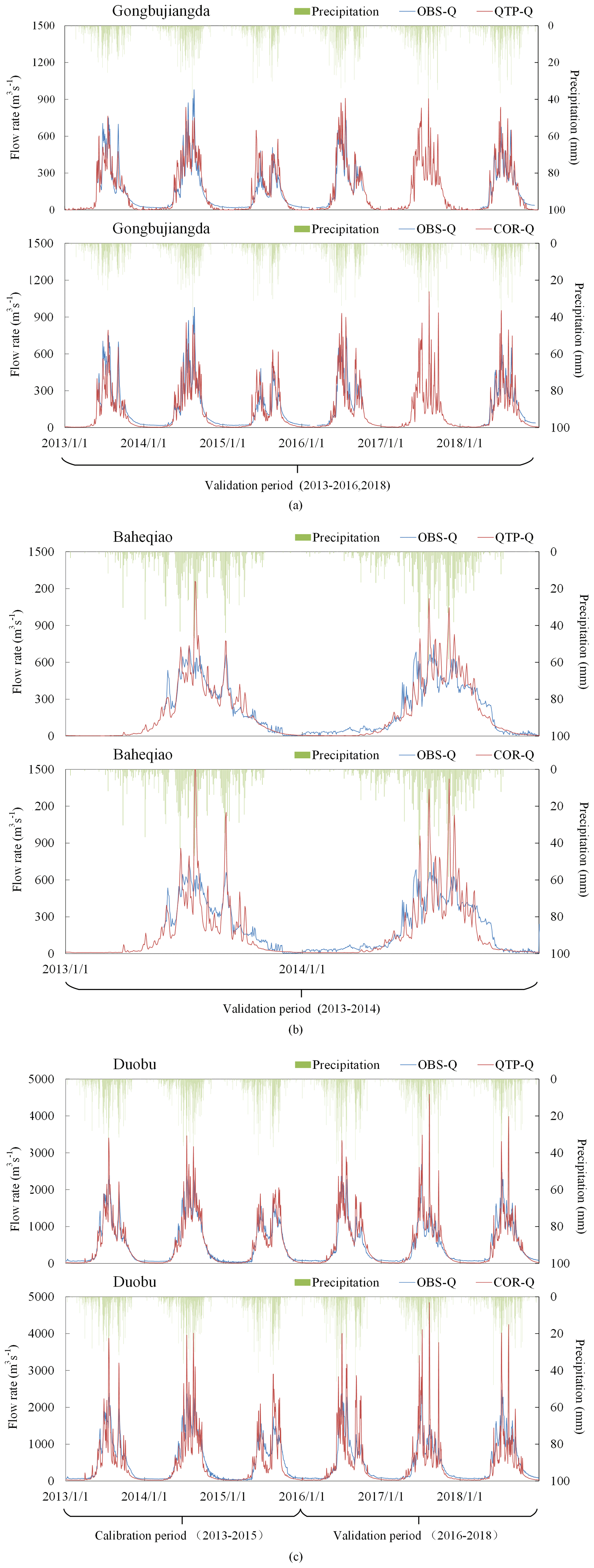
Figure 6 Verification results of the WEP-QTP and WEP-COR models at (a) Duobu, (b) Gongbujiangda, and (c) Baheqiao stations.

Daily flow data from Duobu Station during the calibration and verification periods and from Gongbujiangda and Baheqiao stations during the verification period are shown in Fig. 6 and Table 1. The simulation results of the WEP-QTP model from all three stations were consistent with the measured flow data. During the verification period, compared with the WEP-COR model, the WEP-QTP model showed an increased NSE and a decreased RE, thereby improving the simulation. The WEP-QTP simulation flow process was smoother, and a large flow peak was not easily formed. However, we also found that WEP-QTP underestimated the river discharge during the frozen period; this may be attributed to the model not explicitly considering the outflow of sub-permafrost water, which could supplement the river discharge in the frozen period through macropores in the bedrock fracture zone. In general, the WEP-QTP model delivered an acceptable performance for the Niyang River basin and achieved an NSE > 0.75 and RE < 10 % for the validation period. Hence, the improved model could be used for further analysis.

Table 1 Model validation results for the Gongbujiangda, Baheqiao, and Duobu stations.

3.2 Simulation and comparison of soil–gravel water–heat data at the test sites

Figure 7 shows the air temperature together with the simulated and measured snow thicknesses during freezing and thawing at the experimental site. Snow began to accumulate on 3 December 2016 and was completely melted by 4 April 2017. The maximum snow thickness was 12.4 cm, and the simulated snow thickness was consistent with the measured value.

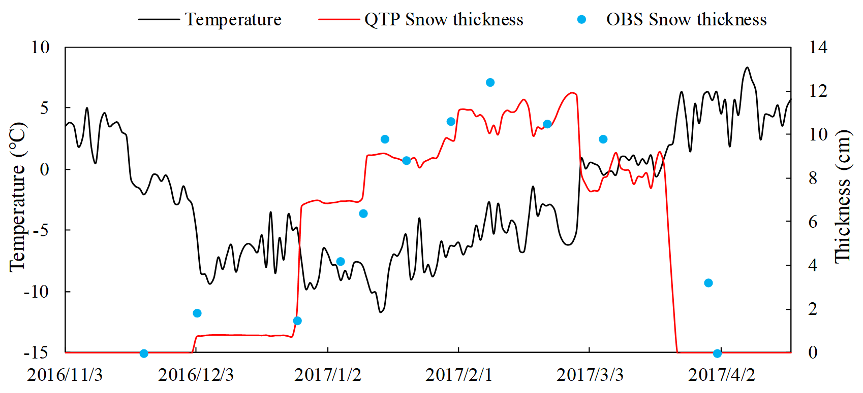
Figure 7 Snow thickness and air temperature during freezing and thawing at the experimental site.

3.2.1 Soil–gravel temperature

The soil–gravel temperature simulation results from the WEP-QTP and WEP-COR models are shown in Fig. 8. The surface soil thickness at the experimental site was approximately 40 cm. For the 10 cm s-layer, because the simulation parameters of the WEP-QTP and WEP-COR models were the same, the simulated temperature results were consistent, except for during the snow cover period (i.e., the period when the snow thickness was > 5 cm between 27 December 2016 and 20 March 2017). Because of the insulation effect of snow, the heat transfer and temperature fluctuations of the surface soil were reduced. The RMSE of WEP-QTP in the 10 cm s-layer was 1.09 ^∘C during the snow cover period; this was much less than the 2.12 ^∘C of WEP-COR. The simulation results of the two models in the 20 cm layer did not differ considerably. For the 40 cm layer and below, the soil in the WEP-COR model had a higher water content than the g-layer in the WEP-QTP model during the early stage of freezing, masking the difference in simulated temperature between the two models (the volumetric heat capacity of water is higher than that of gravel and soil). However, as the temperature decreased, the moisture in the s-layer was converted into ice with a smaller heat capacity; thus, the difference in thermodynamic properties between the s-layer and the g-layer increased gradually. During this period, the simulated difference between the two models reached a maximum of 1.41 ^∘C (40 cm layer, 26 January 2017).

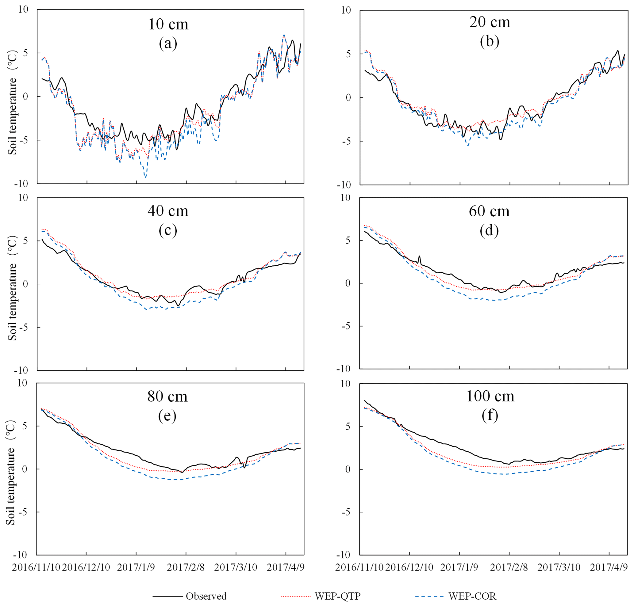
Figure 8 Simulated (WEP-QTP and WEP-COR models) and observed temperatures of the soil–gravel layer at different depths.

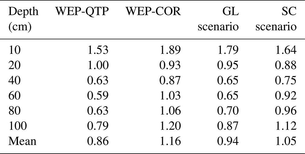
We also compared the simulation results of the scenario considering only the g-layer (“GL Scenario”) with those of the scenario considering only snow cover (“SC Scenario”) to quantitatively analyze how snow and gravel affect the simulation results (Table 2). From Table 2, for the average RMSE, WEP-QTP < GL Scenario < SC Scenario < WEP-COR. Compared with the WEP-COR model, both snow and gravel improved the accuracy of temperature simulation, but the locations of their main effects on heat transfer were different. The RMSE of the SC Scenario at depths of 10–20 cm was smaller than that of the GL Scenario. Snow cover reduces the heat transfer and temperature fluctuations of the surface layer, which improves the simulation accuracy of the surface soil temperature. For depths of 40 cm and below, the RMSE of the GL Scenario was smaller than that of the SC Scenario, and the influence of the g-layer was dominant. Overall, the addition of the snow layer reduced the temperature fluctuations in the surface soil and, in conjunction with the g-layer, corrected the overestimation of the freeze–thaw rate present in the original model. The temperature RMSE was reduced from 1.16 to 0.86 ^∘C.

Table 2 RMSE values for the simulation of temperature (^∘C).

3.2.2 Soil–gravel moisture

Figure 9 shows a comparison between the simulated and measured values of the liquid water content during the freeze–thaw period of the WEP-QTP and WEP-COR models at the experimental site in 2016–2017. After entering the freeze–thaw period, the water in the soil started to freeze from the top layer to the bottom layer as the atmospheric temperature dropped, thereby decreasing the liquid water content layer by layer until February. When the temperature increased in March, the upper layer initially began to thaw, thereby increasing the liquid water content and subsequently thawing the lower layer. At the end of the freeze–thaw period, the upper part of the soil–gravel layer had a higher water content than that in the lower part owing to the infiltration of snowmelt; this water content was also higher than that prior to freezing.

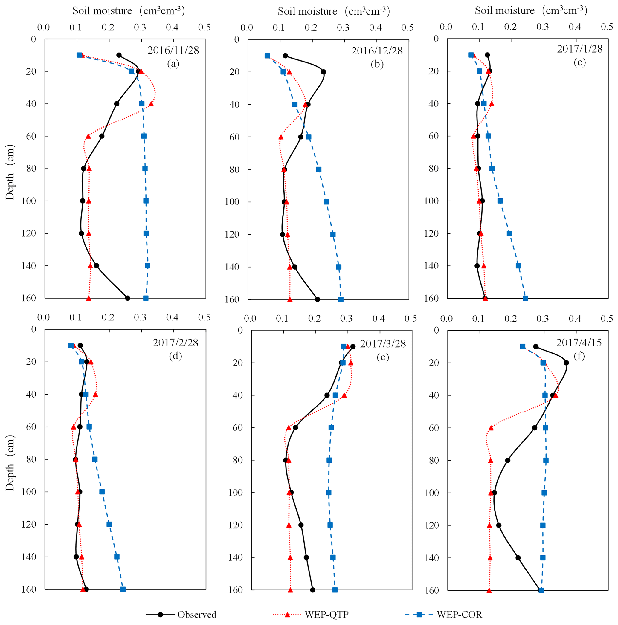
Figure 9 Simulated (WEP-QTP and WEP-COR models) and observed moisture contents of the soil–gravel layer during the freezing and thawing periods.

Over the entire freeze–thaw period, the lower g-layer did not affect the simulation of soil moisture content at a depth of 10 cm. For the 20 and 40 cm depth s-layers, their water-holding capacity was greater than that of the g-layer; hence, their moisture simulated by the WEP-QTP model was greater than that simulated by the WEP-COR model. Below 40 cm depth, the simulation difference between the two models began to emerge more clearly. The simulated moisture of the WEP-COR model varies linearly in the vertical direction and was greater than the measured values, while the moisture simulated by the WEP-QTP model was lower and more similar to the measured values. This can be attributed to the fact that the thickness of the s-layer at the experimental site was 40 cm, and below it was the g-layer with higher hydraulic conductivity and lower water-holding capacity. The WEP-COR model did not take into account the influence of the stratified geological structure on water migration. However, because the actual condition of the underlying surface cannot be homogeneous as assumed in the model generalization, there was a discrepancy in the model simulation results. Soil with a low gravel content may be present at a depth of approximately 160 cm. In March and April after the snow melts, the snowmelt water infiltrated to this depth and was more likely to reside here, and the measured water content value of this layer was between the simulated values of the WEP-QTP and WEP-COR models. The average RE of WEP-COR was 33.74 %, and that of WEP-QTP was smaller, at −12.11 %. Hence, the WEP-QTP model could reflect the influence of gravel on the vertical migration of water.

It should be pointed out that the model improvement is mainly concerned with the water and heat transfer within the seasonal thaw layer, coupled with the fact that the amount of evaporation during the freeze–thaw period is generally less and the latent heat of evaporation accounts for a small proportion of the net radiation. Therefore, the model simplified the calculation of the energy input to the upper boundary of the seasonal thaw layer by using the temperature difference between the atmosphere and the surface as the only source of heat conduction, without quantitatively considering the influence of sensible heat and latent heat of evaporation on the heat flux conducted into the ground. The model needs to be further improved in subsequent studies by systematically considering the influence of the radiation and climate characteristics of the QTP on each energy component.

3.3 Analysis of the snow–soil–gravel layer structure effects on the process of water cycling

To explore the influence of the snow–soil–gravel layer structure on the process of water cycling and the reasons behind the improvement of the model simulation, 2014 (a year for which all measured data were available) was selected as a typical year to compare and analyze the simulation results before and after model improvement (Fig. 10). The simulation difference between the two models became clear from June to October. Compared to the whole year, the difference between the RMSEs of the two models was largest from June to September, and that between the REs of the two models was largest in October (Table 3). For the Gongbujiangda, Baheqiao, and Duobu stations, the RMSEs of WEP-QTP decreased by 14.44, 62.81, and 149.12 m³ s⁻¹, respectively, from June to September, and the absolute values of RE decreased by 4.08 %, 32.67 %, and 45.50 %, respectively, in October. The simulation performance of the WEP-QTP model was better than that of the WEP-COR in three aspects. The peak value of the flood season was not too high, the trough value of the flow process was higher than that of WEP-COR, and the WEP-QTP model showed a better “tailing” process (a slow flow-reduction process consistent with observed flows) from September onwards.

Table 3 Statistical values of the WEP-QTP and WEP-COR models for flow simulations in different periods.

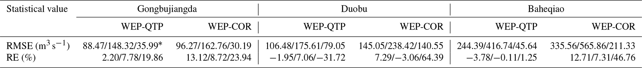
^∗ Values of the whole year, June to September, and October, respectively.

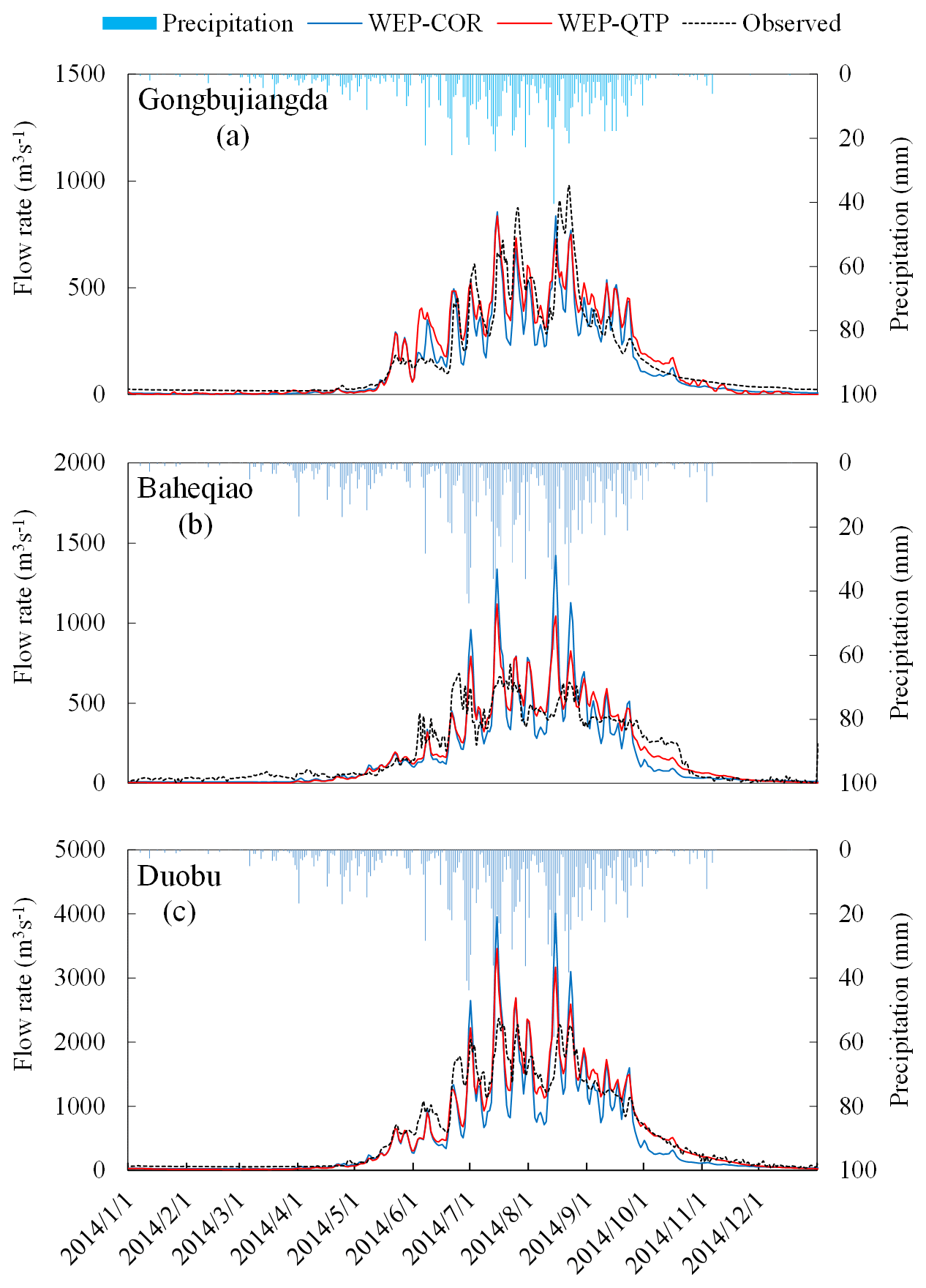
Figure 10 Simulated (WEP-QTP and WEP-COR models) and observed flow rates at the (a) Gongbujiangda, (b) Baheqiao, and (c) Duobu stations in 2014.

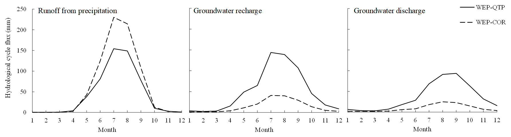
Figure 11 Monthly changes in hydrological cycle flux simulated by the WEP-QTP and WEP-COR models.

By comparing the hydrological cycle fluxes simulated by the two models, the influence of gravel on hydrological processes and the contribution of gravel to enhancing the simulation can be revealed to some extent. Figure 11 shows the comparison and analysis of hydrological cycle flux changes across the basin simulated using the WEP-QTP and WEP-COR models. From June to September, the surface runoff from precipitation simulated by WEP-QTP decreased by 32 % when compared with that simulated by WEP-COR; correspondingly, groundwater recharge and groundwater discharge increased by 249 % and 280 %, respectively. Precipitation during heavy rainfall events in the WEP-QTP model preferentially recharged groundwater via macropores in the g-layer and then recharged the river through groundwater discharge. However, in the WEP-COR model, most of this precipitation contributed to the peak flow during the flood season by the way of surface runoff, which far exceeded the measured value of the flow (Fig. 10). This may be the main reason for the better performance of the WEP-QTP model in the peak and trough flow simulations during the flood season.

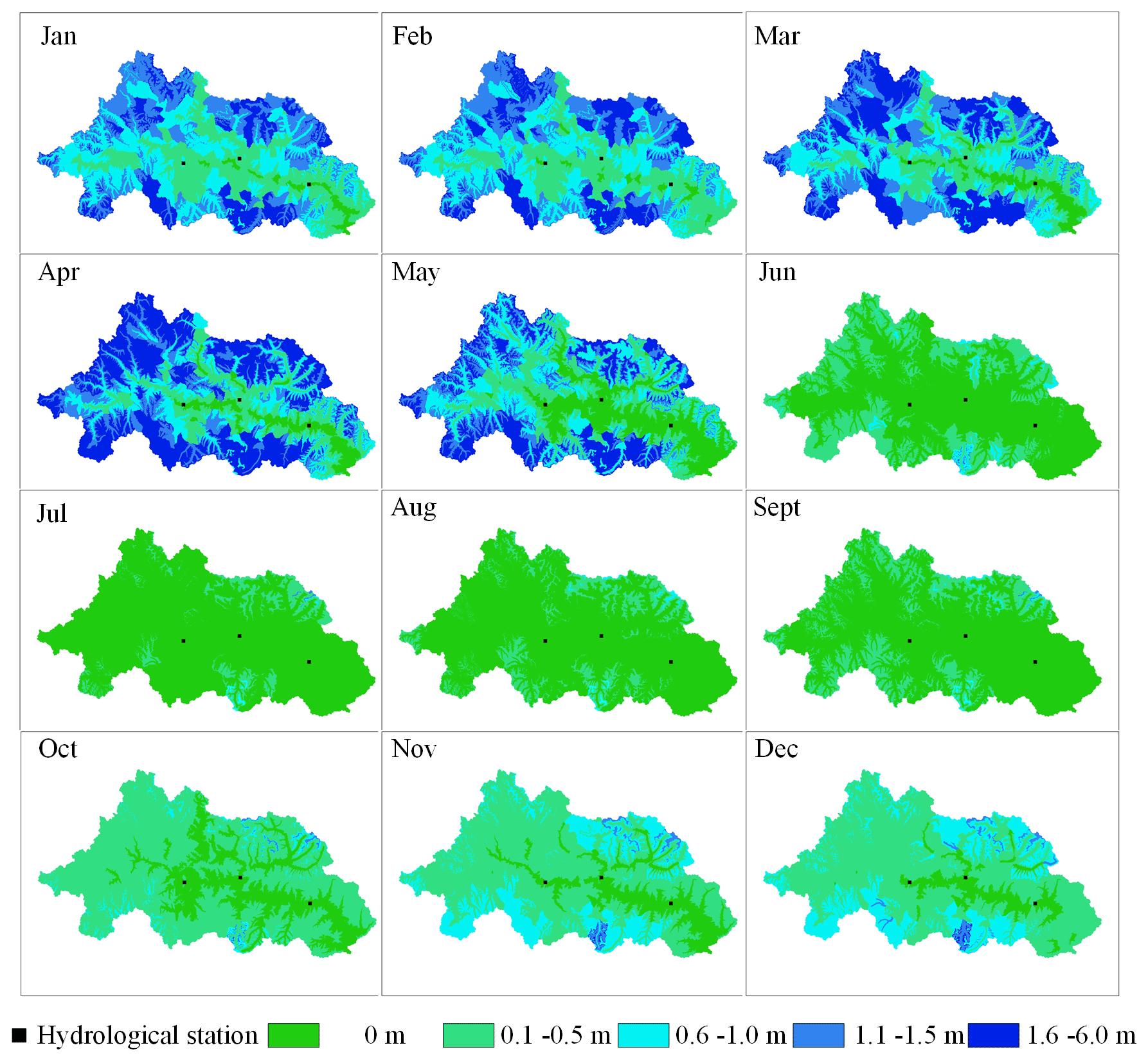
Figure 12 Spatiotemporal variation in snow cover thickness in 2014.

Figure 13 Monthly changes in frozen soil area proportion within the basin.

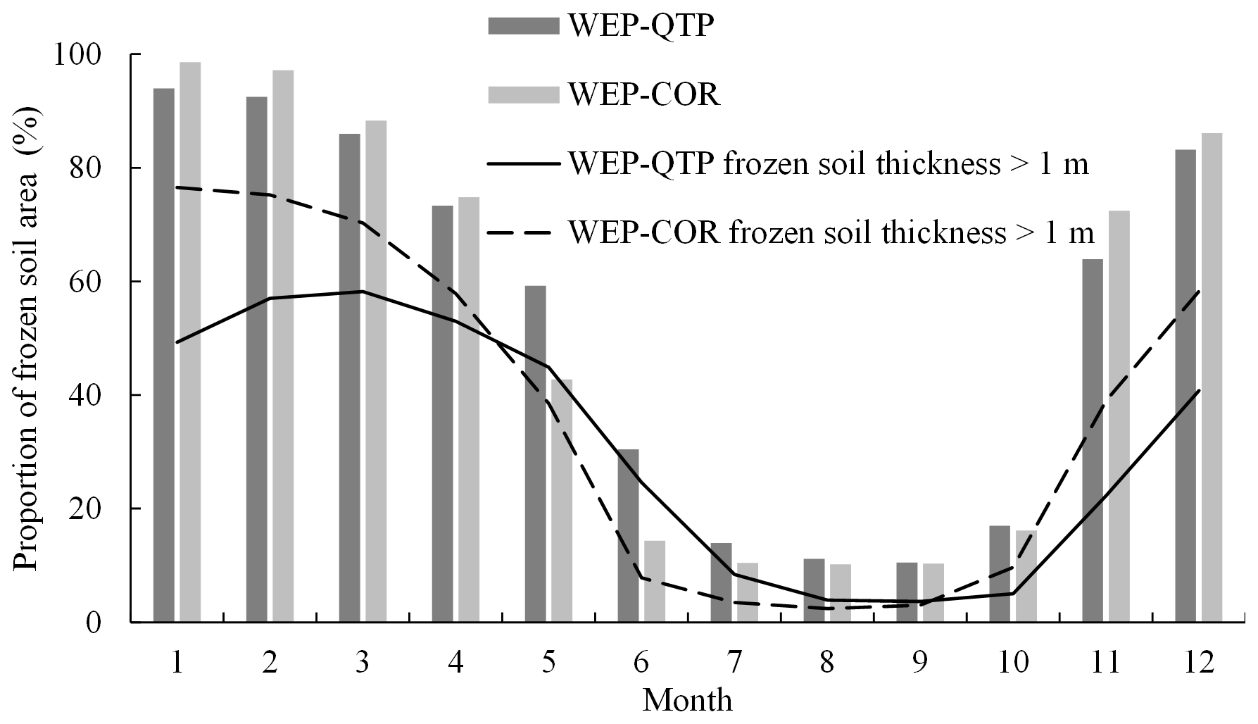
The addition of the snow layer not only reduced the temperature fluctuation of the surface soil, but also, aided by the g-layers, revised the overestimation of the freeze–thaw speed present in the original model. In the lower-elevation valleys (< 4600 $\mathrm{m}\mathrm{a}.\mathrm{s}.\mathrm{l}.$), the percentage of area with a snow thickness > 0.5 m reached its maximum (18 %) in February and then decreased to 0 % by June. However, in high-altitude areas (> 4600 $\mathrm{m}\mathrm{a}.\mathrm{s}.\mathrm{l}.$), where the temperature was lower than that in the valleys, the percentage of area with a snow thickness > 0.5 m reached its maximum (51 %) in April and then dropped to a minimum of 1 % in July (Fig. 12). The WEP-COR model did not consider snow cover, the upper boundary was the atmosphere, and the soil responded quickly to changes in atmospheric temperature. From January to December, the proportion of area with a frozen thickness > 1 m simulated by the WEP-COR model decreased and then increased with changing temperature (maximum in January, minimum in August). In contrast, the proportion of area with a frozen soil thickness > 1 m simulated by the WEP-QTP model reached a maximum in February and a minimum in September (Fig. 13). The inconsistency in the spatiotemporal variation of the frozen soil led to discrepancies in groundwater recharge and discharge processes between the two models. The change in frozen soil area simulated by the WEP-QTP model lagged that simulated by the WEP-COR model, as did the groundwater discharge process (the groundwater discharge of WEP-QTP reached its maximum in September, while that of WEP-COR occurred in August, Fig. 11). Water in the WEP-QTP model had more time to complete groundwater and river recharge and thus exhibited a better tailing process than that in the WEP-COR model (Fig. 10).

In cold regions, climate change affects high and low river flows in different ways. As warming and wetting progresses, changes in high flows show spatial heterogeneity, while low flows show a consistently increasing trend (Song et al., 2021). Warming enhances subsurface flow connectivity and increases groundwater flow by increasing the thickness of the active layer (St. Jacques and Sauchyn, 2009; Walvoord and Kurylyk, 2016). As the medium connecting groundwater and surface water, the water–heat transport of the active layer has a substantial influence on the process of water cycling in cold regions (Chen et al., 2014; Kurylyk et al., 2014). When simulating the water cycle process in the QTP, it is not appropriate to simply generalize the active layer as a homogeneous soil structure and to ignore the influence of g-layers beneath the soil layers. This study shows that, in terms of heat transfer, snow and gravel block heat conduction and slow down the freezing and thawing rates of aquifers. For water transfer, the large pores of the lower g-layer increase the regulation effect of groundwater on flow processes. Under future climate conditions, the participation of groundwater in the water cycle of the QTP may be greater than we expected. Ignoring the snow–soil–gravel layer structure will affect hydrological forecasting, reservoir regulation, and water resource utilization.

4 Conclusions

This study took the Niyang River basin as the study area and constructed the WEP-QTP model on the basis of the original WEP-COR model. The improved WEP-QTP model focuses on the geological structural characteristics of the QTP, dividing a uniform soil profile into two types of media: the upper s-layer and the lower g-layer. When no phase change occurred in the ground, two infiltration models based on a dualistic soil–gravel structure were developed using the Richards equation for non-heavy rain scenarios and the multilayer Green–Ampt model for heavy rain scenarios. During the freeze–thaw period, a water–heat coupling model based on a snow–soil–gravel structure was constructed. This model was used to simulate the process of water cycling within the Niyang River basin, and the improvement of the model was analyzed via comparison with the WEP-COR model.

Compared with the simulation results prior to improvement, the addition of snow not only reduced the surface soil temperature fluctuations, but also interacted with the g-layers to reduce the soil freezing and thawing speed. The underestimation of temperature by WEP-COR was corrected, while the temperature RMSE was reduced from 1.16 to 0.86 ^∘C. Furthermore, the WEP-QTP model was able to reflect the impact of the g-layer on the vertical movement of water and accurately describe the dynamic changes in moisture in the s-layer and the g-layer; the RE of the moisture content was reduced from 33.74 % to −12.11 %.

According to the comparison of the WEP-QTP simulation and measured data from the main stations in the Niyang River basin, the daily flow process simulated by the improved model was more accurate (NSE > 0.75 and |RE| < 10 %), representing a considerable improvement over the WEP-COR model. During the fully thawed period, the dualistic soil–gravel structure increased the recharge and discharge of groundwater and improved the regulation effect of groundwater on flow, thereby stabilizing the water flow process. The maximum RE at the flow peak and trough decreased by 88.2 % and 21.3 %, respectively. During the freeze–thaw period, by considering the effect of the snow–soil–gravel layer continuum on soil freezing and thawing processes, changes in frozen soil depth simulated by WEP-QTP lagged behind those simulated by WEP-COR by approximately 1 month. As a result, there was more time for the river to be recharged by groundwater, as indicated by a better observed tailing process from September onwards.

In contrast to typical cold regions, the widespread geological structure of the QTP changes the process of water cycling in the basin. Ignoring the influence of the dualistic soil–gravel structure greatly impacts hydrological forecasting and water resource assessment.

Appendix A: Distribution of major hydrologically relevant features in the basin

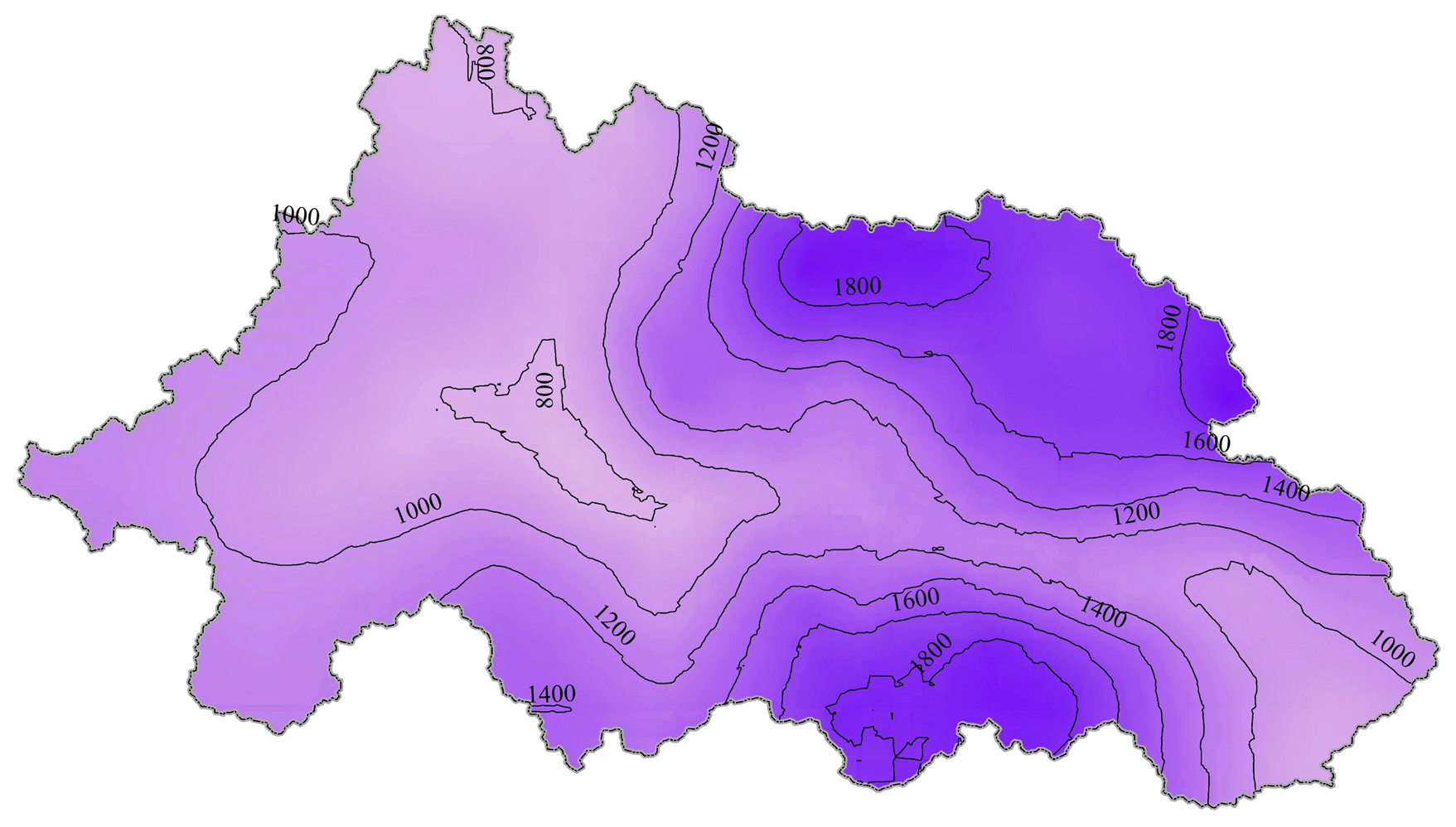
Figure A1 Annual precipitation contour map (mm yr⁻¹).

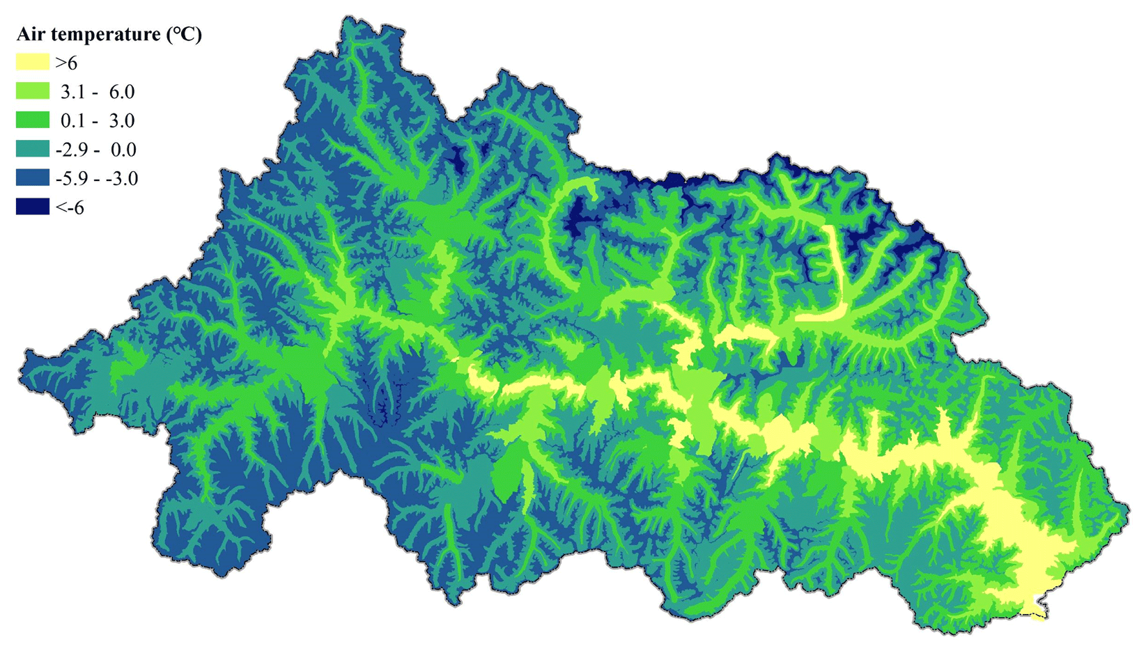
Figure A2 Mean annual temperature (^∘C).

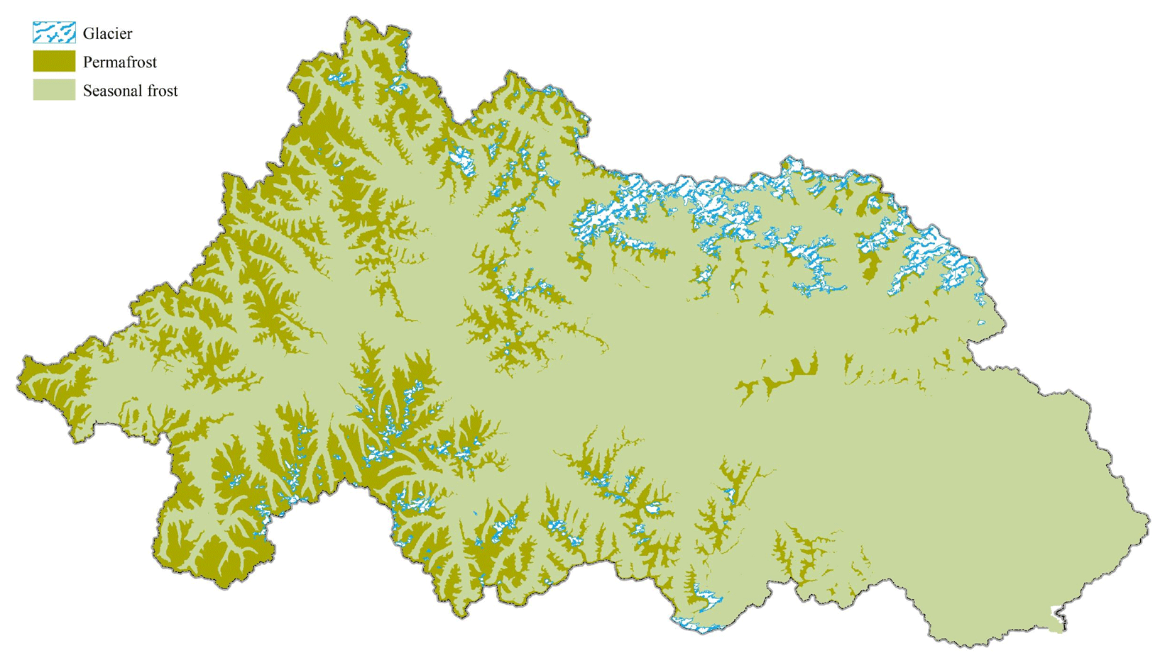
Figure A3 Glacier and permafrost distributions.

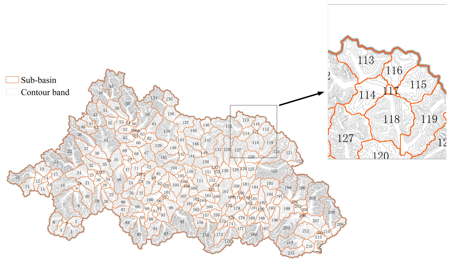
Figure A4 Division of contour bands.

Appendix B: Introduction of the WEP-COR model

The WEP-QTP model was developed based on the water and energy transfer processes in cold regions (WEP-COR) model. To allow better understanding and comparison, the WEP-COR model is briefly introduced in this section.

B1 Model structure

The WEP-COR model is a distributed hydrological model. In terms of the horizontal structure, the WEP-COR model uses the contour bands inside small subbasins as the basic calculation unit (Fig. B1a) and fully considers the vertical changes in vegetation, soil, air temperature, precipitation, and other factors in the basin with changing elevation. Each unit was classified as one of five types according to the type of land use: water body, soil–vegetation, irrigated farmland, non-irrigated farmland, and impervious area. Evapotranspiration of water and soil was calculated using the Penman formula, and the vegetation canopy evaporation was calculated using the Penman–Monteith formula (Monteith, 1973). For soil moisture, the Green–Ampt infiltration model was used for heavy rain periods (Jia and Tamai, 1998), and non-heavy rain periods were simulated using the Richards equation (Jia et al., 2009). The subsurface runoff was calculated based on slope and soil hydraulic conductivity, and groundwater movement was calculated using Boussinesq's equation (Zaradny, 1993). The groundwater outflow was calculated according to the hydraulic conductivity of the riverbed material and the difference between the river water stage and groundwater level (Jia et al., 2001). For glacier-covered areas, the “degree-day factor method” (Hock, 1999) was used to calculate the quantity of glacier melting, and the runoff from the melting of glaciers was directly added to the corresponding hydrological calculation unit.

The vertical structure of the WEP-COR model was divided into the vegetation canopy or building interception, surface depression storage, aeration, transition zone, and groundwater layers. To accurately simulate the changes in soil moisture and heat from the surface to the deep layers and to reflect the influence of soil depth on the evaporation of bare soil and water absorption and transpiration of vegetation roots, the aerated-zone soil was divided into 11 layers (Fig. B1b). The thickness of layers 1–2 was set to 10 cm, and the thickness of layers 3–11 was set to 20 cm.

Figure B1 Horizontal (a) and vertical (b) structures of the WEP-COR model.

B2 Water–heat transport simulation

The WEP-COR model divides soil infiltration into two scenarios: heavy rain infiltration and non-heavy rain infiltration, according to the different runoff-generation mechanisms. In the non-heavy rain infiltration scenario, the runoff is generated by saturation excess, and the soil vertical water flux transfer can be written as follows (Shang et al., 1997; Wang et al., 2014).

$$\begin{array}{}\text{(B1)}& {\displaystyle \frac{\partial {\mathit{\theta }}_{\mathrm{l}}}{\partial t}}={\displaystyle \frac{\partial }{\partial z}}\left[D\left({\mathit{\theta }}_{\mathrm{l}}\right){\displaystyle \frac{\partial {\mathit{\theta }}_{\mathrm{l}}}{\partial z}}-K\left({\mathit{\theta }}_{\mathrm{l}}\right)\right]-{\displaystyle \frac{{\mathit{\rho }}_{\mathrm{I}}}{{\mathit{\rho }}_{\mathrm{l}}}}{\displaystyle \frac{\partial {\mathit{\theta }}_{\mathrm{I}}}{\partial t}}\end{array}$$

θ_l is the volumetric content of liquid water in the soil layer (cm³ cm⁻³), D(θ_l) and K(θ_l) are the unsaturated soil hydraulic diffusivity (cm² s⁻¹) and hydraulic conductivity (cm s⁻¹), respectively, t and z are the time and space coordinates (positive vertically downward), respectively, and ρ_l is the water density (kg m⁻³).

The Van Genuchten function (Van Genuchten, 1980) was used to describe the upper soil water retention curves:

$$\begin{array}{}\text{(B2)}& {\displaystyle \frac{{\mathit{\theta }}_{\mathrm{l}}-{\mathit{\theta }}_{\mathrm{r}}}{{\mathit{\theta }}_{\mathrm{s}}-{\mathit{\theta }}_{\mathrm{r}}}}={\displaystyle \frac{\mathrm{1}}{[\mathrm{1}+(\mathit{\alpha }h{)}^n{]}^m}},\end{array}$$

where θ_s is the saturated water content (cm³ cm⁻³), θ_r is the residual water content (cm³ cm⁻³), h is the matrix suction (cm), α is an empirical parameter (cm⁻¹), n and m are empirical parameters affecting the shape of the retention curve, and $m=\mathrm{1}-\mathrm{1}/n$.

The hydraulic conductivity was calculated using the Mualem model (Mualem, 1986):

$$\begin{array}{}\text{(B3)}& K\left({\mathit{\theta }}_{\mathrm{l}}\right)=\left\{\begin{array}{ll}{K}_{\mathrm{s}}& {\mathit{\theta }}_{\mathrm{l}}={\mathit{\theta }}_{\mathrm{s}}\\ K_{\mathrm{s}}{\left(\frac{{\mathit{\theta }}_{\mathrm{l}}-{\mathit{\theta }}_{\mathrm{r}}}{{\mathit{\theta }}_{\mathrm{s}}-{\mathit{\theta }}_{\mathrm{r}}}\right)}^{\mathrm{\Omega }}& {\mathit{\theta }}_{\mathrm{l}}\ne {\mathit{\theta }}_{\mathrm{s}}\end{array}\right.,\end{array}$$

where K (θ_l) is the hydraulic conductivity (cm s⁻¹) of the soil layer when the liquid water content is θ_l, K_s is the saturated hydraulic conductivity of the soil temperature correction (cm s⁻¹), and Ω is Mualem's constant.

In the heavy rain infiltration scenario, the runoff is generated by infiltration excess. The multilayer unsteady-rainfall Green–Ampt model proposed by Jia and Tamai was used (Jia and Tamai, 1998) to calculate the infiltration process. When the infiltration front (INF) reached the mth layer of the soil, the soil infiltration capacity was calculated using the following formulas.

$$\begin{array}{}\text{(B4)}& {\displaystyle }f=k_{\mathrm{m}}(\mathrm{1}+{\displaystyle \frac{A_{m-\mathrm{1}}}{B_{m-\mathrm{1}}+F}})\text{(B5)}& {\displaystyle }{A}_{m-\mathrm{1}}=\left(\sum _{\mathrm{1}}^{m-\mathrm{1}}{L}_i-\sum _{\mathrm{1}}^{m-\mathrm{1}}{\displaystyle \frac{L_i{k}_{\mathrm{m}}}{k_i}}+{\mathrm{SW}}_{\mathrm{m}}\right)\mathrm{\Delta }{\mathit{\theta }}_{\mathrm{m}}\text{(B6)}& {\displaystyle }{B}_{m-\mathrm{1}}=\left(\sum _{\mathrm{1}}^{m-\mathrm{1}}{\displaystyle \frac{L_i{k}_{\mathrm{m}}}{k_i}}\right)\mathrm{\Delta }{\mathit{\theta }}_{\mathrm{m}}-\sum _{\mathrm{1}}^{m-\mathrm{1}}{L}_i\mathrm{\Delta }{\mathit{\theta }}_i\end{array}$$

f is the infiltration capacity (mm h⁻¹), A_m−1 is the total water capacity of the soil above the m layer (mm), B_m−1 is the error caused by the different soil moisture contents of the soil above the m layer (mm), F is the cumulative infiltration (mm), k_i is the hydraulic conductivity of the ith soil layer (mm h⁻¹), L_i is the soil thickness of the ith layer (mm), SW_m is the capillary suction pressure at the INF of the mth layer (mm), and $\mathrm{\Delta }{\mathit{\theta }}_i={\mathit{\theta }}_{\mathrm{s}}-{\mathit{\theta }}_{\mathrm{l}}$.

The cumulative infiltration quantity F when the INF reached the mth layer was calculated based on whether there was water accumulation on the ground surface. If the ground surface had accumulated water when the INF reached the m−1th layer, Eq. (B7) was used; otherwise, Eq. (B8) was used.

$$\begin{array}{}\text{(B7)}& {\displaystyle }\begin{array}{rl}F-F_{m-\mathrm{1}}=& k_{\mathrm{m}}(t-t_{m-\mathrm{1}})+A_{m-\mathrm{1}}\\ & \times \text{ln}\left({\displaystyle \frac{A_{m-\mathrm{1}}+B_{m-\mathrm{1}}+F}{A_{m-\mathrm{1}}+B_{m-\mathrm{1}}+F_{m-\mathrm{1}}}}\right)\end{array}\text{(B8)}& {\displaystyle }\begin{array}{rl}F-F_{\mathrm{p}}=& k_{\mathrm{m}}(t-t_{\mathrm{p}})+A_{m-\mathrm{1}}\\ & \times \text{ln}\left({\displaystyle \frac{A_{m-\mathrm{1}}+B_{m-\mathrm{1}}+F}{A_{m-\mathrm{1}}+B_{m-\mathrm{1}}+F_{\mathrm{p}}}}\right)\end{array}\text{(B9)}& {\displaystyle }{F}_{m-\mathrm{1}}=\sum _{\mathrm{1}}^{m-\mathrm{1}}{L}_i\mathrm{\Delta }{\mathit{\theta }}_i\text{(B10)}& {\displaystyle }{F}_{\mathrm{p}}=A_{m-\mathrm{1}}\left({\displaystyle \frac{I_{\mathrm{p}}}{k_{\mathrm{m}}}}-\mathrm{1}\right)-B_{m-\mathrm{1}}\text{(B11)}& {\displaystyle }{t}_{\mathrm{p}}=t_{m-\mathrm{1}}+(F_{\mathrm{p}}-F_{n-\mathrm{1}})/I_{\mathrm{p}}\end{array}$$

t is the time, t_m−1 is the time when the INF reaches the interface between the m−1 and m layers, t_p is the start time of the water accumulation, F_p is the cumulative infiltration quantity at t_p, and I_p is the precipitation intensity at t_p.

The relationship between the water and heat transport of frozen soil is mainly manifested in the dynamic balance of the moisture content of the unfrozen water and the negative temperature of the soil. According to the principle of energy balance, the energy change in each layer in the freeze–thaw system was used for the soil temperature change and water phase change in the system. The heat flux conducted into the soil was calculated using the forced recovery method (Douville et al., 1995; Pitman et al., 1991). The heat flux and temperature of each layer were calculated using the following equations (Chen et al., 2008):

$$\begin{array}{}\text{(B12)}& {\displaystyle }{H}_{i,i+\mathrm{1}}=\mathrm{0.1782}{\displaystyle \frac{({\mathit{\lambda }}_i{Z}_i+{\mathit{\lambda }}_{i+\mathrm{1}}{Z}_{i+\mathrm{1}})(T_i-T_{i+\mathrm{1}})}{(Z_i+Z_{i+\mathrm{1}}{)}^{\mathrm{2}}}}\text{ and}\text{(B13)}& {\displaystyle }{T}_i={\displaystyle \frac{H_{i-\mathrm{1},i}-H_{i,i+\mathrm{1}}}{C_{\mathrm{V}i}{Z}_i}}.\end{array}$$

i is the number of soil layers, $H_{i,i+\mathrm{1}}$ represents the sensible heat flux between the i layer and the i+1 layer (MJ m⁻²), λ represents the thermal conductivity ($\mathrm{W}(\mathrm{m}{}^{\circ }\mathrm{C}{)}^{-\mathrm{1}}$), Z is the thickness (cm), C_V is the soil volume heat capacity ($\mathrm{J}({\mathrm{m}}^{\mathrm{3}}{}^{\circ }\mathrm{C}{)}^{-\mathrm{1}}$), and T is the temperature (^∘C).

Temperature is the driving force of the water phase change. The relationship between the water and heat transport of frozen soil is mainly manifested in the dynamic balance of the moisture content of the unfrozen water and the negative temperature of the soil (Wang et al., 2014; Niu and Yang, 2006):

$$\begin{array}{}\text{(B14)}& {\mathit{\theta }}_{\mathrm{l}}={\mathit{\theta }}_{\mathrm{m}}\left(T\right),\end{array}$$

where θ_m(T) is the maximum unfrozen water moisture content corresponding to a negative soil temperature.

For further details of the WEP-COR model, please refer to Li et al. (2019).