When best is the enemy of good – critical evaluation of performance criteria in hydrological models

Performance criteria play a key role in the calibration and evaluation of hydrological models and have been extensively developed and studied, but some of the most used criteria still have unknown pitfalls. This study set out to examine counterbalancing errors, which are inherent to the Kling–Gupta efficiency (KGE) and its variants. A total of nine performance criteria – including the KGE and its variants, as well as the Nash–Sutcliffe efficiency (NSE) and the modified index of agreement (d₁) – were analysed using synthetic time series and a real case study. Results showed that, when assessing a simulation, the score of the KGE and some of its variants can be increased by concurrent overestimation and underestimation of discharge. These counterbalancing errors may favour bias and variability parameters, therefore preserving an overall high score of the performance criteria. As bias and variability parameters generally account for two-thirds of the weight in the equation of performance criteria such as the KGE, this can lead to an overall higher criterion score without being associated with an increase in model relevance. We recommend using (i) performance criteria that are not or less prone to counterbalancing errors (d₁, modified KGE, non-parametric KGE, diagnostic efficiency) and/or (ii) scaling factors in the equation to reduce the influence of relative parameters.

1 Introduction

Hydrological models are fundamental to solving problems related to water resources. They help characterise hydrosystems (Hartmann et al., 2014), predict floods (Kauffeldt et al., 2016; Jain et al., 2018), and manage water resources (Muleta and Nicklow, 2005). A lot of research efforts are thus dedicated to improving the reliability, the robustness, and the relevance of such models. Improvements can be made by working on (i) input data, (ii) model parameters and structure, (iii) uncertainty quantification, (iv) model calibration (Beven, 2019), and also (v) appropriate benchmarks for assessing model performance (Seibert et al., 2018). In this study, we focus on the proper use of performance criteria for calibrating and evaluating hydrological models – an important part that can easily be overlooked (Jackson et al., 2019).

A performance criterion aims to evaluate the goodness of fit of a model to observed data. It is generally expressed as a score, for which the best value corresponds to a perfect fit between predictions and observations. In hydrology, the Nash–Sutcliffe efficiency (NSE) (Nash and Sutcliffe, 1970) is still one of the most commonly used criteria (Kling et al., 2012), although the past decade has seen a gain in popularity of alternatives (Clark et al., 2021), e.g. the Kling–Gupta efficiency (KGE) (Gupta et al., 2009). Many authors have pointed out the inherent limitations of using performance criteria, especially the fact that a single-score metric cannot reflect all relevant hydrological aspects of a model (Gupta et al., 2009). The use of a multi-criteria framework is thus often emphasised to quantify different aspects of a model (Clark et al., 2021; Moriasi et al., 2015; Gupta et al., 1998; Jackson et al., 2019; van Werkhoven et al., 2009; Knoben et al., 2019; Althoff and Rodrigues, 2021; Ritter and Muñoz-Carpena, 2013; Krause et al., 2005; Legates and McCabe, 1999) alongside a scientific evaluation of the results (Biondi et al., 2012). Knoben et al. (2019), Althoff and Rodrigues (2021), and Clark et al. (2021) pointed out that modellers should carefully think about which aspects they consider to be the most important in their hydrological model and how to evaluate them. In relation to the assessment of model performance, Seibert et al. (2018) argued that the current benchmarks poorly reflect what could and should be expected of a model. They suggested that one should define lower and upper benchmarks based on the performance of a simple bucket-type model with few parameters using the same data set.

Performance criteria also have shortcomings at a distinctive level. A number of studies have identified several limitations of the NSE: (i) the contribution of the normalised bias depends on the discharge variability of the basin; (ii) discharge variability is inevitably underestimated because the NSE is maximised when the variability equals the correlation coefficient, which is always smaller than unity; and (iii) mean flow is not a meaningful benchmark for highly variable discharges (Gupta et al., 2009; Willmott et al., 2012). The KGE aims to address these limitations but also has its own issues (Gupta et al., 2009). Santos et al. (2018) identified pitfalls when using the KGE with a prior logarithmic transformation of the discharge. Knoben et al. (2019) warned against directly comparing NSE and KGE scores as the KGE has no inherent benchmark. Ritter and Muñoz-Carpena (2013) and Clark et al. (2021) showed that NSE and KGE scores can be strongly influenced by few data points, resulting in substantial uncertainties in the predictions.

What is not fully addressed yet is the trade-off between individual components (Wöhling et al., 2013) and especially the impact of counterbalancing errors induced by bias and variability parameters, which are integrated in many performance criteria. While accurate bias and variability are desired aspects of hydrological models, sometimes good evaluations may accidentally result from negative and positive values cancelling each other (Jackson et al., 2019; Massmann et al., 2018). This can be particularly detrimental to model calibration and evaluation as it generates an increase in the criterion score without necessarily being associated with a better model relevance. Some performance criteria naturally address this problem by using absolute or squared error values, but other criteria such as the KGE and its variants do not as they use relative errors. The aim of this study is to assess the extent to which criteria scores can be trusted for calibrating and evaluating hydrological models when predictions have concurrent over- and underestimated values. The influence of counterbalancing errors is evaluated on nine performance criteria including the NSE and KGE. This selection is far being from exhaustive but includes widely used and recently proposed KGE variants, as well as more traditional criteria such as the NSE or the modified index of agreement (d₁) for comparison purposes. We first use synthetic time series to highlight the counterbalancing-errors mechanism. Second, we show how counterbalancing errors can impair the interpretation of hydrological models in a real case study. Finally, we provide some recommendations about the use of scaling factors and the choice of appropriate performance criteria to nullify or reduce the influence of counterbalancing errors.

2 Performance criteria

2.1 Parameter description

All the performance criteria considered in this study are based on the same or similar statistical indicators, which are first described to avoid repetition.

We use x_o(t) and x_s(t) to refer to observed and simulated values of calibration variable x at a specific time step t; r and r_s correspond to the Pearson and the Spearman rank correlation coefficients (Freedman et al., 2007), respectively.

β is the ratio between the mean of simulated values μ_s and the mean of observed values μ_o:

$$\begin{array}{}\text{(1)}& \mathit{\beta }={\displaystyle \frac{{\mathit{\mu }}_{\mathrm{s}}}{{\mathit{\mu }}_{\mathrm{o}}}}.\end{array}$$

β_n corresponds to the bias (mean error) normalised by the standard deviation of observed values σ_o:

$$\begin{array}{}\text{(2)}& {\mathit{\beta }}_{\mathrm{n}}={\displaystyle \frac{{\mathit{\mu }}_{\mathrm{s}}-{\mathit{\mu }}_{\mathrm{o}}}{{\mathit{\sigma }}_{\mathrm{o}}}}.\end{array}$$

α is the ratio between the standard deviation of simulated values σ_s and the standard deviation of observed values σ_o:

$$\begin{array}{}\text{(3)}& \mathit{\alpha }={\displaystyle \frac{{\mathit{\sigma }}_{\mathrm{s}}}{{\mathit{\sigma }}_{\mathrm{o}}}}.\end{array}$$

γ is the ratio between the coefficient of the variation of simulated values (CV${}_{\mathrm{s}}={\mathit{\sigma }}_{\mathrm{s}}/{\mathit{\mu }}_{\mathrm{s}}$) and the coefficient of the variation of observed values (CV${}_{\mathrm{o}}={\mathit{\sigma }}_{\mathrm{o}}/{\mathit{\mu }}_{\mathrm{o}}$):

$$\begin{array}{}\text{(4)}& \mathit{\gamma }={\displaystyle \frac{{\mathrm{CV}}_{\mathrm{s}}}{{\mathrm{CV}}_{\mathrm{o}}}}.\end{array}$$

${\stackrel{\mathrm{‾}}{B}}_{\mathrm{rel}}$ and |B_area| (Schwemmle et al., 2021) are based on the flow duration curve (FDC). B_rel(i) is defined as the relative bias of the simulated and observed flow duration curves at the exceedance probability i:

$$\begin{array}{}\text{(5)}& B_{\mathrm{rel}}={\displaystyle \frac{x_{\mathrm{s}}\left(i\right)-x_{\mathrm{o}}\left(i\right)}{x_{\mathrm{o}}\left(i\right)}},\end{array}$$

where x_s(i) and x_o(i) correspond to the simulated and observed values of the calibration variable at exceedance probability i. ${\stackrel{\mathrm{‾}}{B}}_{\mathrm{rel}}$ is the mean of B_rel(i) when looking at n observations:

$$\begin{array}{}\text{(6)}& {\stackrel{\mathrm{‾}}{B}}_{\mathrm{rel}}={\displaystyle \frac{\mathrm{1}}{n}}\sum _{i=\mathrm{0}}^{i=\mathrm{1}}{B}_{\mathrm{rel}}\left(i\right).\end{array}$$

|B_area| is calculated as follows:

$$\begin{array}{}\text{(7)}& \left|B_{\mathrm{area}}\right|=\underset{\mathrm{0}}{\overset{\mathrm{1}}{\int }}\left|B_{\mathrm{res}}\left(i\right)\right|\mathrm{d}i,\end{array}$$

with B_res being the residual bias:

$$\begin{array}{}\text{(8)}& B_{\mathrm{res}}=B_{\mathrm{rel}}\left(i\right)-{\stackrel{\mathrm{‾}}{B}}_{\mathrm{rel}}.\end{array}$$

α_NP (Pool et al., 2018) is also based on the FDC:

$$\begin{array}{}\text{(9)}& {\mathit{\alpha }}_{\mathrm{NP}}=\mathrm{1}-{\displaystyle \frac{\mathrm{1}}{\mathrm{2}}}\sum _{k=\mathrm{1}}^n\left|{\displaystyle \frac{x_{\mathrm{s}}\left(I\right(k\left)\right)}{n{\mathit{\mu }}_{\mathrm{s}}}}-{\displaystyle \frac{x_{\mathrm{o}}\left(J\right(k\left)\right)}{n{\mathit{\mu }}_{\mathrm{o}}}}\right|,\end{array}$$

where I(k) and J(k) stand for the time steps of the kth largest discharge for the simulated and observed time series, respectively.

As β, β_n, and ${\stackrel{\mathrm{‾}}{B}}_{\mathrm{rel}}$ all represent the bias, they are therefore designed as bias parameters in this study.

2.2 Score calculation

A total of nine performance criteria are analysed in this study: the NSE, KGE, 2012 version of the KGE or modified KGE (KGE^′), 2021 version of the KGE (KGE^′′), non-parametric KGE (KGE_NP), diagnostic efficiency (DE), Liu mean efficiency (LME), least-squares combined efficiency (LCE), and d₁. The value considered to be the best score is equal to 1 for all criteria, except for the DE, for which it is equal to zero.

The NSE (Nash and Sutcliffe, 1970) is a normalised variant of the mean squared error (MSE) and compares a prediction to the observed mean of the target variable:

$$\begin{array}{}\text{(10)}& \mathrm{NSE}=\mathrm{1}-{\displaystyle \frac{\sum {\left(x_{\mathrm{s}}\left(t\right)-x_{\mathrm{o}}\left(t\right)\right)}^{\mathrm{2}}}{\sum {\left(x_{\mathrm{o}}\left(t\right)-{\mathit{\mu }}_{\mathrm{o}}\right)}^{\mathrm{2}}}}.\end{array}$$

Gupta et al. (2009) algebraically decomposed the NSE into correlation, variability, and bias components:

$$\begin{array}{}\text{(11)}& \mathrm{NSE}=\mathrm{2}\mathit{\alpha }r-{\mathit{\alpha }}^{\mathrm{2}}-{\mathit{\beta }}_{\mathrm{n}}^{\mathrm{2}}.\end{array}$$

The KGE was proposed by Gupta et al. (2009) as an alternative to the NSE. The optimal KGE corresponds to the closest point of the three-dimensional Pareto front – of α, β, and r – to the ideal value of [1; 1; 1]:

$$\begin{array}{}\text{(12)}& \mathrm{KGE}=\mathrm{1}-\sqrt{(\mathit{\alpha }-\mathrm{1}{)}^{\mathrm{2}}+(\mathit{\beta }-\mathrm{1}{)}^{\mathrm{2}}+(r-\mathrm{1}{)}^{\mathrm{2}}}.\end{array}$$

A modified Kling–Gupta efficiency was proposed by Kling et al. (2012). The coefficient of variation is used instead of the standard deviation to ensure that bias and variability are not cross-correlated:

$$\begin{array}{}\text{(13)}& {\mathrm{KGE}}^{\prime }=\mathrm{1}-\sqrt{(\mathit{\gamma }-\mathrm{1}{)}^{\mathrm{2}}+(\mathit{\beta }-\mathrm{1}{)}^{\mathrm{2}}+(r-\mathrm{1}{)}^{\mathrm{2}}}.\end{array}$$

Tang et al. (2021) proposed another variant (KGE^′′) by using the normalised bias instead of β to ensure that the score is not overly sensitive to mean values – μ_o or μ_s – that are close to zero (Santos et al., 2018; Tang et al., 2021):

$$\begin{array}{}\text{(14)}& {\mathrm{KGE}}^{\prime \prime }=\mathrm{1}-\sqrt{(\mathit{\alpha }-\mathrm{1}{)}^{\mathrm{2}}+{\mathit{\beta }}_{\mathrm{n}}^{\mathrm{2}}+(r-\mathrm{1}{)}^{\mathrm{2}}}.\end{array}$$

Pool et al. (2018) cautioned against the implicit assumptions of the KGE – data linearity, data normality, and absence of outliers – and proposed a non-parametric alternative (KGE_NP) for limiting their impact. The non-parametric form of the variability is calculated using the FDC, and the Spearman rank correlation coefficient is used instead of the Pearson correlation coefficient:

$$\begin{array}{}\text{(15)}& {\mathrm{KGE}}_{\mathrm{NP}}=\mathrm{1}-\sqrt{{\left({\mathit{\alpha }}_{\mathrm{NP}}-\mathrm{1}\right)}^{\mathrm{2}}+(\mathit{\beta }-\mathrm{1}{)}^{\mathrm{2}}+{\left(r_{\mathrm{S}}-\mathrm{1}\right)}^{\mathrm{2}}}.\end{array}$$

In a similar way, Schwemmle et al. (2021) used FDC-based parameters to account for variability and bias in another KGE variant: the diagnostic efficiency. This criterion is based on constant, dynamic, and timing errors and aims to provide a stronger link to hydrological processes (Schwemmle et al., 2021):

$$\begin{array}{}\text{(16)}& \mathrm{DE}=\sqrt{{\stackrel{\mathrm{‾}}{B}}_{\mathrm{rel}}^{\mathrm{2}}+{\left|B_{\mathrm{area}}\right|}^{\mathrm{2}}+(r-\mathrm{1}{)}^{\mathrm{2}}}.\end{array}$$

In this study, we used a normalised diagnostic efficiency (DE^′) so that the best error score is equal to 1 for facilitating the comparison with other performance criteria:

$$\begin{array}{}\text{(17)}& {\mathrm{DE}}^{\prime }=\mathrm{1}-\sqrt{{\stackrel{\mathrm{‾}}{B}}_{\mathrm{rel}}^{\mathrm{2}}+{\left|B_{\mathrm{area}}\right|}^{\mathrm{2}}+(r-\mathrm{1}{)}^{\mathrm{2}}}.\end{array}$$

Liu (2020) proposed another alternative, the Liu mean efficiency, to improve the simulation of extreme events. The LME thus aims to address the underestimation of variability of the KGE, which is still a concern despite not being as severe as with the NSE (Gupta et al., 2009; Mizukami et al., 2019):

$$\begin{array}{}\text{(18)}& \mathrm{LME}=\mathrm{1}-\sqrt{(r\mathit{\alpha }-\mathrm{1}{)}^{\mathrm{2}}+(\mathit{\beta }-\mathrm{1}{)}^{\mathrm{2}}}.\end{array}$$

Lee and Choi (2022) proposed the least-squares combined efficiency to address the shortcomings of the LME identified by Choi (2022), namely (i) an infinite number of solutions for the maximum score and (ii) an inclination to overestimate high flows and underestimate low flows. The LCE is based on the least-squares statistics combined from both-way regression lines rα and $r/\mathit{\alpha }$:

$$\begin{array}{}\text{(19)}& \mathrm{LCE}=\mathrm{1}-\sqrt{(r\mathit{\alpha }-\mathrm{1}{)}^{\mathrm{2}}+(r/\mathit{\alpha }-\mathrm{1}{)}^{\mathrm{2}}+(\mathit{\beta }-\mathrm{1}{)}^{\mathrm{2}}}.\end{array}$$

Willmott et al. (1985) proposed a modified index of agreement, which aim to address the issues associated with r and the coefficient of determination, as well as the sensitivity of the original index of agreement to outliers (Legates and McCabe, 1999):

$$\begin{array}{}\text{(20)}& d_{\mathrm{1}}=\mathrm{1}-{\displaystyle \frac{\sum \mathrm{|}{x}_{\mathrm{s}}\left(t\right)-x_{\mathrm{o}}\left(t\right)\mathrm{|}}{\sum \left(\mathrm{|}{x}_{\mathrm{s}}\left(t\right)-{\mathit{\mu }}_{\mathrm{o}}\mathrm{|}+\left|x_{\mathrm{o}}\left(t\right)-{\mathit{\mu }}_{\mathrm{o}}\right|\right)}}.\end{array}$$

Figure 1 Synthetic hydrograph corresponding to two flood events.

3 Synthetic time series

3.1 Generating synthetic time series with homothetic transformations

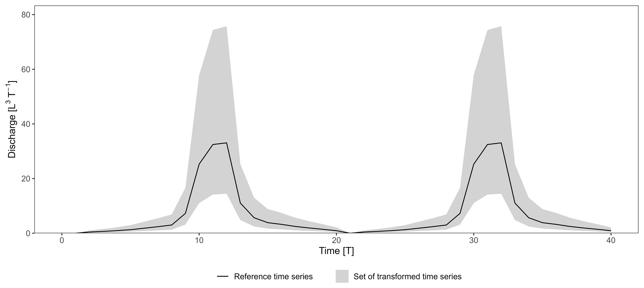
A simulation performance can be assessed in terms of bias, variability, and timing errors (Gupta et al., 2009). Bias and variability errors correspond to a difference in the volume and amplitude of discharges. Timing errors correspond to a shift in time. We created a synthetic hydrograph corresponding to one flood event as the reference (observed) time series. We also generated synthetic transformations – of the reference time series – with different errors in terms of bias and variability corresponding to the time series simulated by a model. We did not consider any timing errors as our aim is to assess counterbalancing errors induced by bias and variability parameters. Synthetic transformations were generated by multiplying the reference time series by the coefficient ω:

$$\begin{array}{}\text{(21)}& Q_{\mathrm{s}}\left(t\right)=Q_{\mathrm{o}}\left(t\right)\cdot \mathit{\omega },\end{array}$$

where Q_s(t) stands for the transformed discharge at the time t, Q_o(t) stands for the reference discharge at the time t, and ω stands for the coefficient. ω values were sampled uniformly on the log-transformed interval [−0.36, 0.36] at a defined step of 0.002 to ensure a fair distribution between underestimated and overestimated transformations. The exponentiation in base 10 of the sampled values results in 361 ω values evenly distributed around the ω=1 homothety, which corresponds to the reference time series (i.e. absence of transformation). We defined ω bounds such that the transformed peak discharge roughly ranges from half ($\mathit{\omega }\approx \mathrm{0.437}\approx {\mathrm{10}}^{-\mathrm{0.36}}$) to twice ($\mathit{\omega }\approx \mathrm{2.291}\approx {\mathrm{10}}^{\mathrm{0.36}}$) that of the reference time series. Note that (i) the data linearity between simulated and observed values is verified and (ii) ω homotheties still induce small timing errors – which were considered to be negligible – because the correlation coefficients (r and r_s) also slightly account for the shape of the transformation.

To study counterbalancing errors induced by bias and variability parameters, we generated time series that consist of two successive flood events and considered all possible combinations of the 361 transformations for the simulated time series (Fig. 1). This results in a total of 361²=130 321 transformations with two flood events, including (i) a perfect transformation with ω=1 for both flood events, (ii) bad–good (BG) or good–bad (GB) transformations when ω=1 for only one out of the two flood events, and (iii) bad–bad (BB) transformations when ω≠1 for both flood events. The performance of the transformations with regards to the reference time series were evaluated using the nine performance criteria presented in Sect. 2.

3.2 Identifying counterbalancing errors on a straightforward example

Figure 2 presents the following two hydrographs extracted from the set of transformations: (i) a BB model with the combination [ω₁=0.75; ω₂=1.2] and (ii) a BG model with the combination [ω₁=0.75; ω₂=1]. The BG model stands out as a better model because it perfectly reproduces the second flood event and is identical to the BB model during the first flood (ω₁=0.75). Nevertheless, the KGE and its variants – KGE^′, KGE^′′, KGE_NP, DE^′, LME, and LCE – all favour the BB model, whereas only the NSE and d₁ evaluate the BG model as better (Fig. 3a). Further results for common and recently developed performance criteria are presented in Fig. A1 in the Appendix.

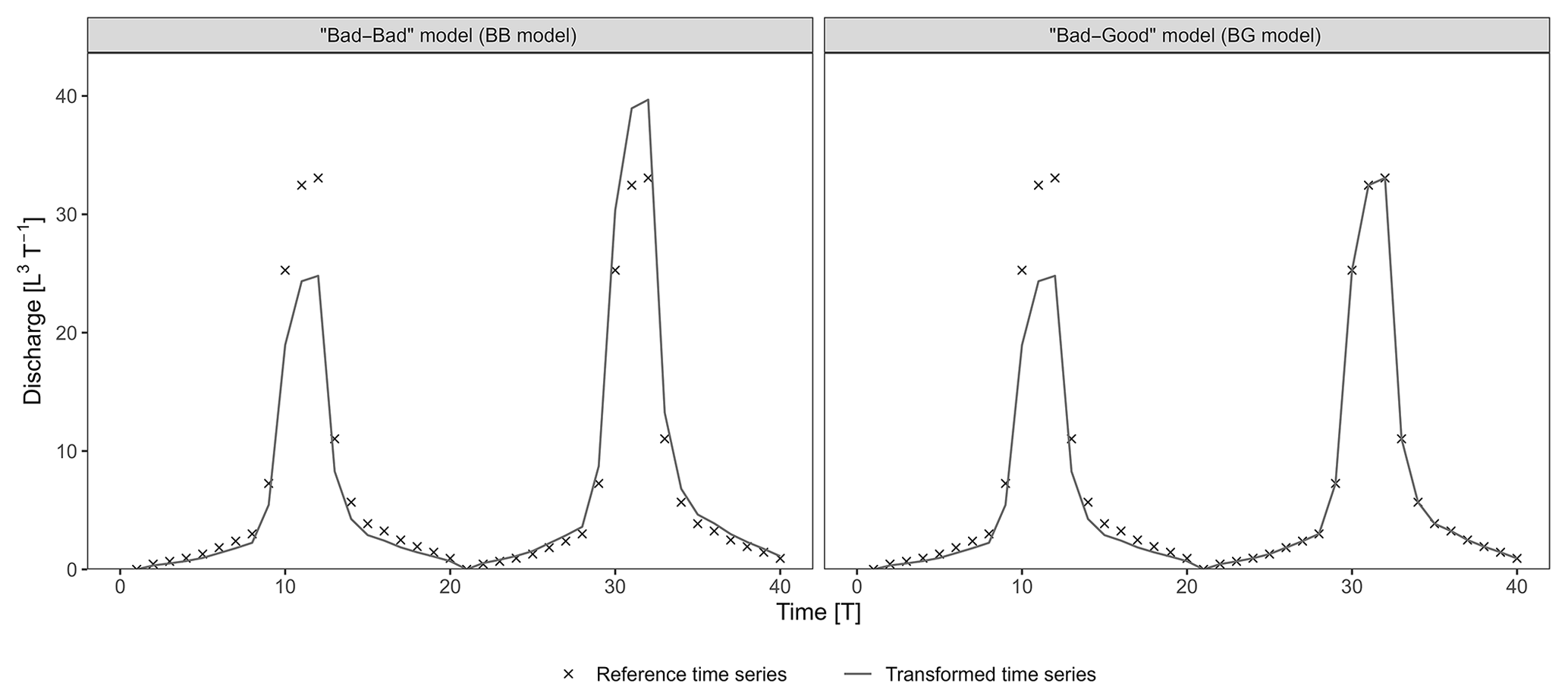
Figure 2 Synthetic examples extracted from the set of transformations. The first and second flood events of the bad–bad and bad–good transformations were shifted with [ω₁=0.75; ω₂=1.2] and [ω₁=0.75; ω₂=1] combinations, respectively.

The investigation of the components of the criteria (Fig. 3b) reveals how a seemingly better model (i.e. the BG model) can have a lower score than expected. Bias parameters are systematically better for the BB model, with 0.98 over 0.88 for β, −0.02 over −0.08  for β_n, and −0.04 over −0.12 for ${\stackrel{\mathrm{‾}}{B}}_{\mathrm{rel}}$. Timing parameters are systematically better for the BG model, with 0.99 over 0.96 for r and 0.99 over 0.98 for r_s. Variability parameters are mixed: (i) α favours the BB model with 1.01 over 0.89, (ii) γ favours the BG model with 1.01 over 1.04, (iii) α_NP slightly favours the BG model with 0.94 over 0.93, and (iv) |B_area| is equal for both models. The rα and $r/\mathit{\alpha }$ parameters are better for the BB model; 2αr is better for the BG model.

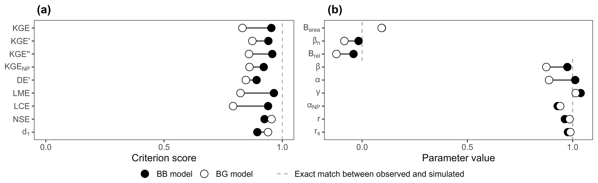
Figure 3 (a) Score of the BB and BG transformations according to the different performance criteria. (b) Values of the parameters used in the calculation of the performance criteria.

The β, β_n, ${\stackrel{\mathrm{‾}}{B}}_{\mathrm{rel}}$, α, rα, and $r/\mathit{\alpha }$ parameters all provide a better evaluation of bias and variability for the BB model. Concurrent over- and underestimation of discharges over the time series result in a good water balance: close to 1 for β and ${\stackrel{\mathrm{‾}}{B}}_{\mathrm{rel}}$ and 0 for β_n. Depending on the criterion, the variability parameter can also affect the score in a similar counter-intuitive manner. α is heavily impacted by the counterbalance, whereas it seems to be mitigated for γ, α_NP, and |B_area|. The timing parameters (r and r_s) have an expected score that favours the BG model. However, the score difference in terms of timing errors between BB and BG models is very small (0.03 at best for r). The impact on the overall score is thus minimised compared to the one induced by bias and variability parameters, which can be cumulated (e.g. both β and α counterbalancing errors in the KGE) or have a larger difference – up to 0.12 for α. Counterbalancing errors can thus result in better values for bias and variability, which increase the overall score. In this case, the highest score may not be the most appropriate indicator of model relevance.

The largest differences in score appear for the LME and LCE criteria as all their parameters are affected by counterbalancing errors (β, rα, and $r/\mathit{\alpha }$). The KGE and KGE^′′ also show significant differences as they accumulate the counterbalancing errors of α and β. The KGE^′ demonstrates a smaller difference than the KGE due to the use of γ. Both FDC-based criteria KGE_NP and DE^′ show the smallest differences due to α_NP and |B_area|, which have a nearly equal value for both BB and BG models. The NSE has a slightly better score on the BG model, while the difference is more pronounced for d₁.

This example demonstrates how relative error metrics can cancel each other out and affect the design and the evaluation of hydrological models. The counterbalancing errors especially affect bias parameters (β, β_n, and ${\stackrel{\mathrm{‾}}{B}}_{\mathrm{rel}}$) but also the variability parameter α.

Figure 4 Score of each transformation for all [ω₁; ω₂] combinations by performance criteria.

3.3 Exploring counterbalancing errors with synthetic transformations

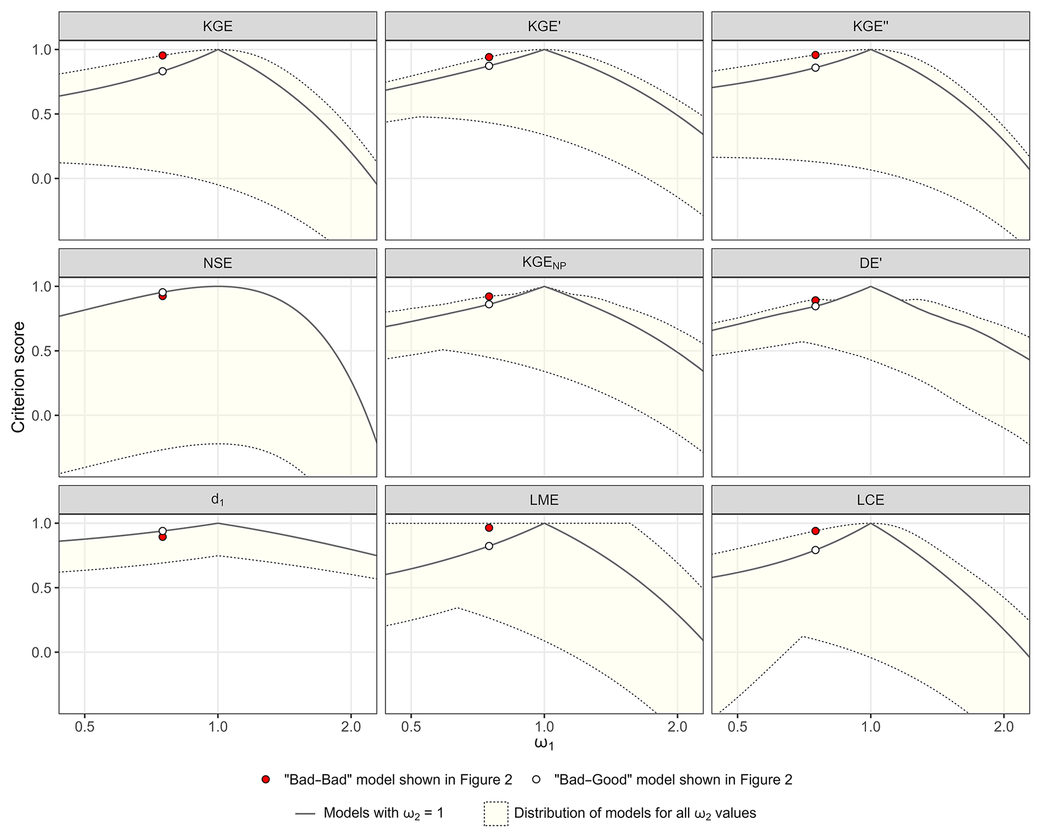
Figure 4 shows the score distribution of the synthetic set of hydrographs presented in Sect. 3.1. For each value of ω₁, the minimum and maximum criteria scores of the transformations resulting from all combinations with ω₂ provide the dashed envelope of the score distribution, with the maximum transformation score at the top (1 corresponding to a perfect model) and the worst at the bottom. The transformations corresponding to the BG models (with ω₂=1) are represented by the black line. All transformations included in the dashed envelope can be identified as bad–bad models, except when ω₁=1 or ω₂=1 (black line).

It is obvious that the KGE and its variants – KGE^′, KGE^′′, KGE_NP, DE^′, LME, and LCE – always evaluate one or several BB models as being better than the BG model for the same ω₁ value, except for ω₁=1. On the other hand, the NSE and d₁ correctly identify the BG model as the best transformation for all combinations of [ω₁; ω₂]; i.e. the black line is always above the dashed envelope. The envelopes of the KGE, KGE^′, and KGE^′′ criteria are similar, but they do not display the same difference between the best scores and the scores of the BG models. These differences are smaller for the latter two because the KGE^′ is based on γ instead of α, and the KGE^′′ is based on β_n instead of β, for which it is demonstrated in Sect. 3.2 that they both soften counterbalancing errors. The envelope of the LCE criterion looks like that of the KGE. However, the difference between the best scores and the scores of the BG models is much higher. This is likely due to the nature of the equation consisting of three parameters affected by counterbalancing errors (β, rα, and $r/\mathit{\alpha }$). The LME criterion has a very distinctive envelope, for which the maximum score of 1 is reached for a lot of BB models, even when both ω₁ and ω₂ are different from 1. This can be explained by the interaction between r and α that leads to an infinite number of solutions (Choi, 2022). The KGE_NP and DE^′ (FDC-based criteria) both show similar envelopes with a break point near the maximum transformation score in both directions around ω₁=1. This is especially pronounced for the DE^′, for which the BG model is nearly the best model between ω₁=0.83 and ω₁=1.17. These results show that counterbalancing errors can happen on a large range of parameters, and when using the KGE or its variants, there is a possibility for the more meaningful model (i.e. BG model) to have a lower score than a compensated or bad–bad model.

Figure 5 shows the value of ω₂ corresponding to the best evaluation for a given ω₁ by performance criteria. As identified above, the NSE and d₁ both evaluate the BG models as the best transformations (NSE and d₁ black lines coincide at ω₂=1, Fig. 5). Counterbalancing errors are apparent for the KGE and its variants. For ω₁≠1, the best transformations are always BB models and follow two conditions: (i) if ω₁<1 then ω₂>1, and (ii) if ω₁>1 then ω₂<1. This means that, in this case, such performance criteria will always be flawed towards concurrent under- and overestimation of discharges in a transformation.

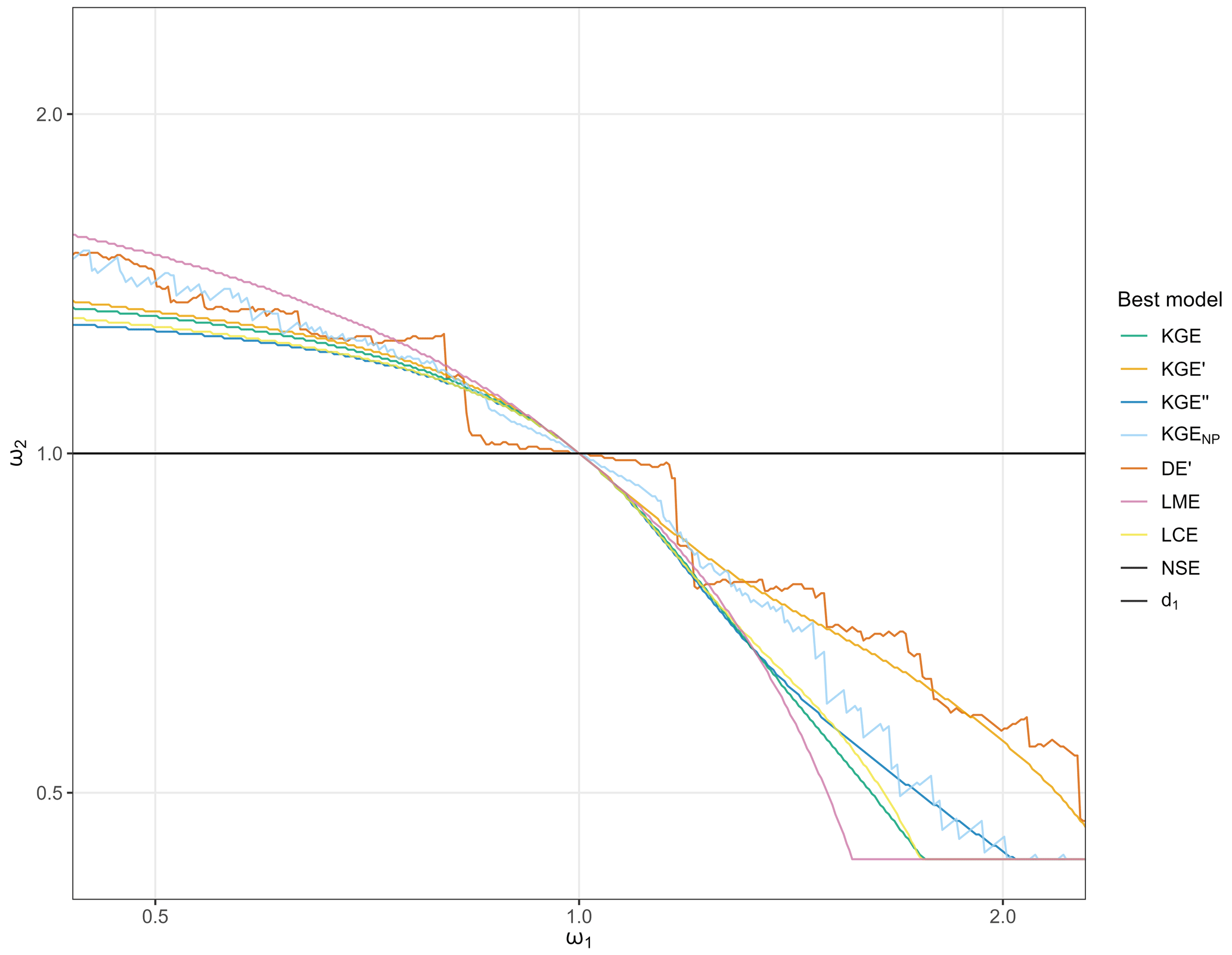
Figure 5 Graph of each [ω₁; ω₂] combination identified as the best transformation by each performance criteria. The NSE and d₁ black lines coincide at ω₂=1.

4 Real case study

To highlight how counterbalancing errors can affect the assessment of hydrological models in a real case study, we used two different modelling approaches: artificial neural networks (ANNs) and bucket-type models. The simulations of the karst spring discharges of both models were evaluated for the same 1-year validation period. To clearly highlight the problem, we deliberately chose a bucket-type simulation that is noticeably affected by counterbalancing errors yet is still realistic. Further information on the modelling approaches, the input data, the calibration strategy, and the simulation procedure can be found in Cinkus et al. (2023).

4.1 Study site

The Unica springs are the outlet of a complex karstic system influenced by a network of poljes. The recharge area is about 820 km² and is located in a moderate continental climate with a strong snow influence. Recharge comes from both (i) allogenic infiltration from two sub-basins drained by sinking rivers and (ii) autogenic infiltration through a highly karstified limestone plateau (Gabrovšek et al., 2010; Kovačič, 2010; Petric, 2010). The network of connected poljes constitutes a common hydrological entity that induces a high hydrological variability in the system and long and delayed high discharges at the Unica springs (Mayaud et al., 2019). The limestone massif can reach a height of 1800 m a.s.l. (above sea level) and has significant groundwater resources (Ravbar et al., 2012). A polje downstream of the springs can flood when the Unica discharge exceeds 60 m³ s⁻¹ for several days. If the flow reaches 80 m³ s⁻¹, the flooding can reach the gauging station and influence its measurement. The flow data are from the gauging station in Unica-Hasberg (ARSO, 2021a). Precipitation, height of snow cover, and height of new snow data are from the meteorological stations in Postojna and Cerknica (ARSO, 2021b). Temperature and relative humidity data are from the Postojna station. Potential evapotranspiration is calculated from the Postojna station data with the Penman–Monteith formula (Allen et al., 1998).

4.2 Modelling approaches

The first modelling approach is based on convolutional neural networks (CNNs) (LeCun et al., 2015), which is a specific type of ANN that is powerful in processing image-like data but also very useful for processing sequential data. The model consists of a single 1D convolutional layer with a fixed kernel size of 3 and an optimised number of filters. This layer was complemented by a MAX-POOLING LAYER, a Monte Carlo dropout layer with 10 % dropout rate and two dense layers. The first dense layer had an optimised number of neurons, and the second layer had a single output neuron. We programmed our models in Python 3.8 (van Rossum, 1995) using the following frameworks and libraries: Bayesian optimisation (Nogueira, 2014), Matplotlib (Hunter, 2007), NumPy (van der Walt et al., 2011), Pandas (Reback et al., 2021; McKinney, 2010), scikit-learn (Pedregosa et al., 2018), TensorFlow 2.7 (Abadi et al., 2016), and Keras API (Chollet, 2015).

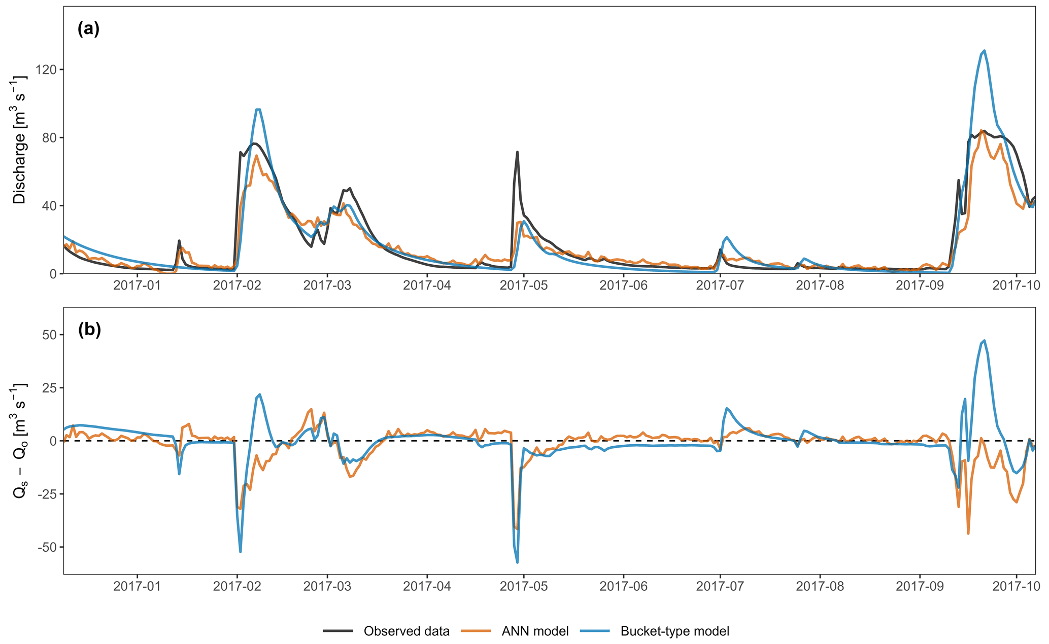
Figure 6 (a) Observed and simulated spring discharge time series for the validation period. (b) Relative difference between simulated and observed discharge for the validation period.

The second modelling approach is a bucket-type model, which is a conceptual representation of a hydrosystem consisting of several buckets that are supposed to be representative of the main processes involved. We used the adjustable modelling platform KarstMod (Mazzilli et al., 2019). The model structure consists of one upper bucket for simulating soil and epikarst processes (including a soil available water capacity) and two lower buckets corresponding to matrix and conduits compartments. A very reactive transfer function from the upper bucket to the spring is used to reproduce very fast flows occurring in the system.

4.3 Impact of counterbalancing errors on model evaluation

Figure 6a shows the results of the two hydrological models for Unica springs. The models have overall good dynamics and successfully reproduce the observed discharges. Regarding high-flow periods, both models show a small timing error, inducing a delay in the simulated peak flood. The first flood event (February 2017) is slightly underestimated by the ANN model and highly overestimated by the bucket-type model. The second flood event (March 2017) is similarly underestimated by both models, but the bucket-type model demonstrates a slightly better performance. The third flood event (May 2017) is poorly simulated by the models, with both underestimating the flood peak, but the ANN model is more accurate in terms of timing and volume estimate, while the bucket-type model has a better recession coefficient and flow variability. The last flood event (September 2017) comprise a small peak followed by a very high and long-lasting flood. Both models fail to account for the small peak. The following important flood event is highly overestimated by the bucket-type model while being nicely simulated by the ANN model despite the small underestimation and timing error. The small flood events are better simulated by the ANN model than the bucket-type model: (i) the ANN model simulates them satisfactorily, except for the second one (mid-April), where the simulated discharges are overestimated; (ii) the bucket-type model does not simulate the first two events at all (mid-January and mid-April) and largely overestimates the last two (early and late June) in addition to timing errors. Both models can be improved during recession and low-flow periods. The ANN model is rather close to the observed discharges but seems to be too sensitive to precipitation (continuous oscillations). On the other hand, the bucket-type model shows no oscillations but either overestimates or underestimates the observed discharges. Some events are not well simulated by both models (e.g. the May 2017 flood), which may be due to uncertainties in the input data. Also, the data linearity between simulated and observed values is slightly skewed for both models, which can affect the relevance of r (Barber et al., 2020).

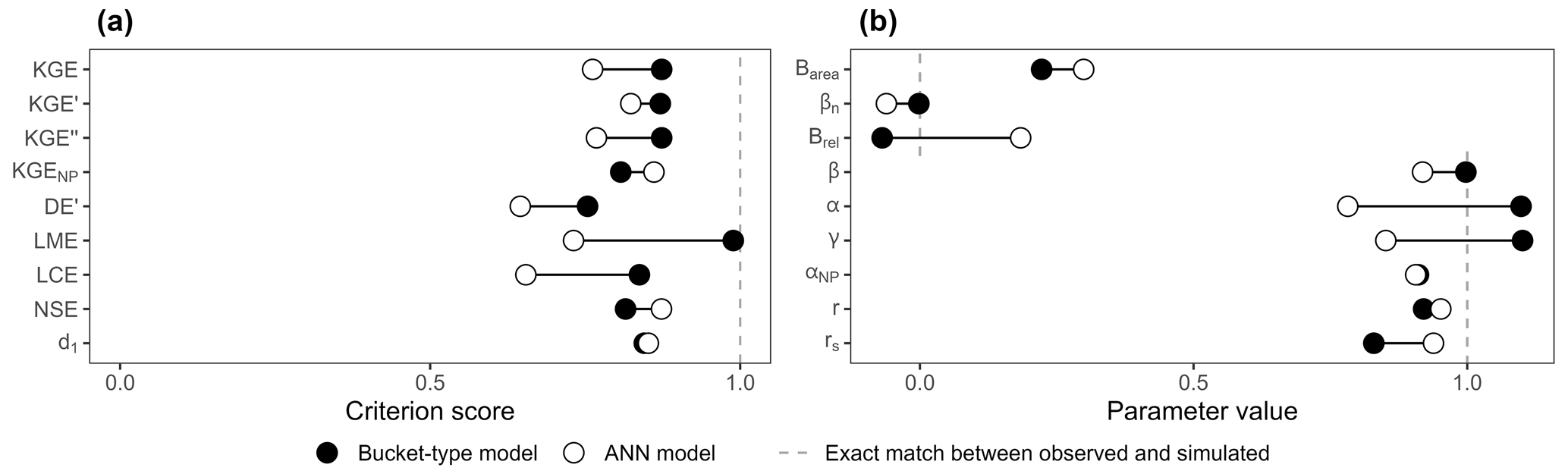
Figure 7 (a) Score of the ANN and bucket-type models according to the different performance criteria. (b) Values of the parameters used in the calculation of the performance criteria.

In general, the ANN model can be described as better because it is closer to the observed values in the high- and low-flow periods. While this statement cannot be supported by performance metrics, we believe that an expert assessment based on intuition and experience is still valuable despite being intrinsically subjective. In this particular case, one can assess the main, distinctive flaws of each model: (i) the ANN model has continuous oscillations – especially during recession and low-flow periods – and lacks accuracy during recession periods; (ii) the bucket-type model highly overestimates several flood events and is inaccurate during a lot of recession and low-flow periods. Figure 6b also shows that the bucket-type model has an overall higher bias than the ANN model. Hydrological models are generally used for (i) the prediction or forecast of water flooding or inrush, (ii) the management of water resources, (iii) the characterisation of hydrosystems, and more recently (iv) the study of the impact of climate change on water resources. Most studies thus put the emphasis on volumes and also on extremes events (i.e. dry and flood periods), which in this case are more satisfactorily reproduced by the ANN model in terms of volume estimate, timing, and variability.

This visual assessment is confirmed by only a few performance criteria: the NSE, d₁, and KGE_NP (Fig. 7a). These criteria evaluate the ANN model as better, although the performances of both models are quite close for the d₁. However, the KGE and most of its variants (except the KGE_NP) all favour the bucket-type model over the ANN model – sometimes by a large margin. Further results for common and recently developed performance criteria are presented in Fig. A2 in the Appendix. It is interesting to note how similar these results are to those of the synthetic example (Figs. 3a and A1 in the Appendix). Looking at the values of the equations' parameters (Fig. 7b), we find that bias parameters are systematically better for the bucket-type model, with 1 over 0.92 for β, 0 over −0.06 for β_n, and −0.07 over 0.18 for ${\stackrel{\mathrm{‾}}{B}}_{\mathrm{rel}}$. Timing errors are systematically better for the ANN model, with 0.95 over 0.92 for r and 0.94 over 0.83 for r_s. Variability parameters favour the bucket-type model with 1.1 over 0.78 for α, 1.1 over 0.85 for γ, 0.22 over 0.3 for |B_area|, and a very close value that is better by 0.005 for the α_NP parameter. In summary, all bias and variability parameters have better values for the bucket-type model, while timing and shape parameters are better for the ANN model.

As the KGE and its variants are generally composed of equally weighted bias, variability, and timing, their overall score is heavily affected by compensation effects – except in the case of a large error for one parameter. In our case, all parameters have similar errors, which results in a better KGE for the bucket-type model compared to the ANN model. This applies to all the KGE variants except the KGE_NP, where the error for r_s is significant, resulting in a better score for the ANN model. The LME score is extremely high (0.99) for the bucket-type model, which is probably due to the compensation of r and α identified by Choi (2022). Also, using γ instead of α for assessing the variability seems to lower counterbalancing errors.

Interestingly, the cumulative sum of the absolute bias error between simulated and observed values (Fig. 6b) is smaller for the ANN model (1394 m³) than the bucket-type model (1611 m³), but still the relative bias and variability parameters are better for the bucket-type model. This observation highlights how counterbalancing errors can impair the evaluation of hydrological models: seemingly better parameters values (bias and variability) that increase criteria scores are not necessarily associated with an increase in model relevance.

5 Recommendations

The aim of this paper is primarily to raise awareness among modellers. Performance criteria generally aggregate several aspects of the characteristics of a model into a single value, which can lead to an inaccurate assessment of said aspects. Ultimately, all criteria have their flaws and should be carefully selected with regards to the aim of the model.

5.1 Use of relevant performance criteria

Table 1 summarises the presence and impact of counterbalancing errors, as well as the advantages and drawbacks (as reported in other studies) of the different performance criteria. The recommendations for counterbalancing errors are based on the results of this research – i.e. synthetic and real case studies. The KGE and all its variants are affected by counterbalancing errors with varying degrees of intensity: (i) mildly impacted (+) for the KGE^′, KGE_NP, and DE; (ii) moderately impacted ($++$) for the KGE, KGE^′′, and LCE; and (iii) strongly impacted ($+++$) for the LME. In this study, the NSE and d₁ stand out as clearly better since they have no counterbalancing errors. However, they have other drawbacks that are not associated with counterbalancing errors, especially the NSE, with its limitations related to variability (Gupta et al., 2009). We thus recommend using performance criteria that are not or less prone to counterbalancing errors (d₁, KGE^′, KGE_NP, DE).

Table 1 Presence and impact of counterbalancing errors (CEs) on the assessment of model performance according to different performance criteria. The impact of CEs is denoted as null (–), mild (+), moderate ($++$), or strong ($+++$).

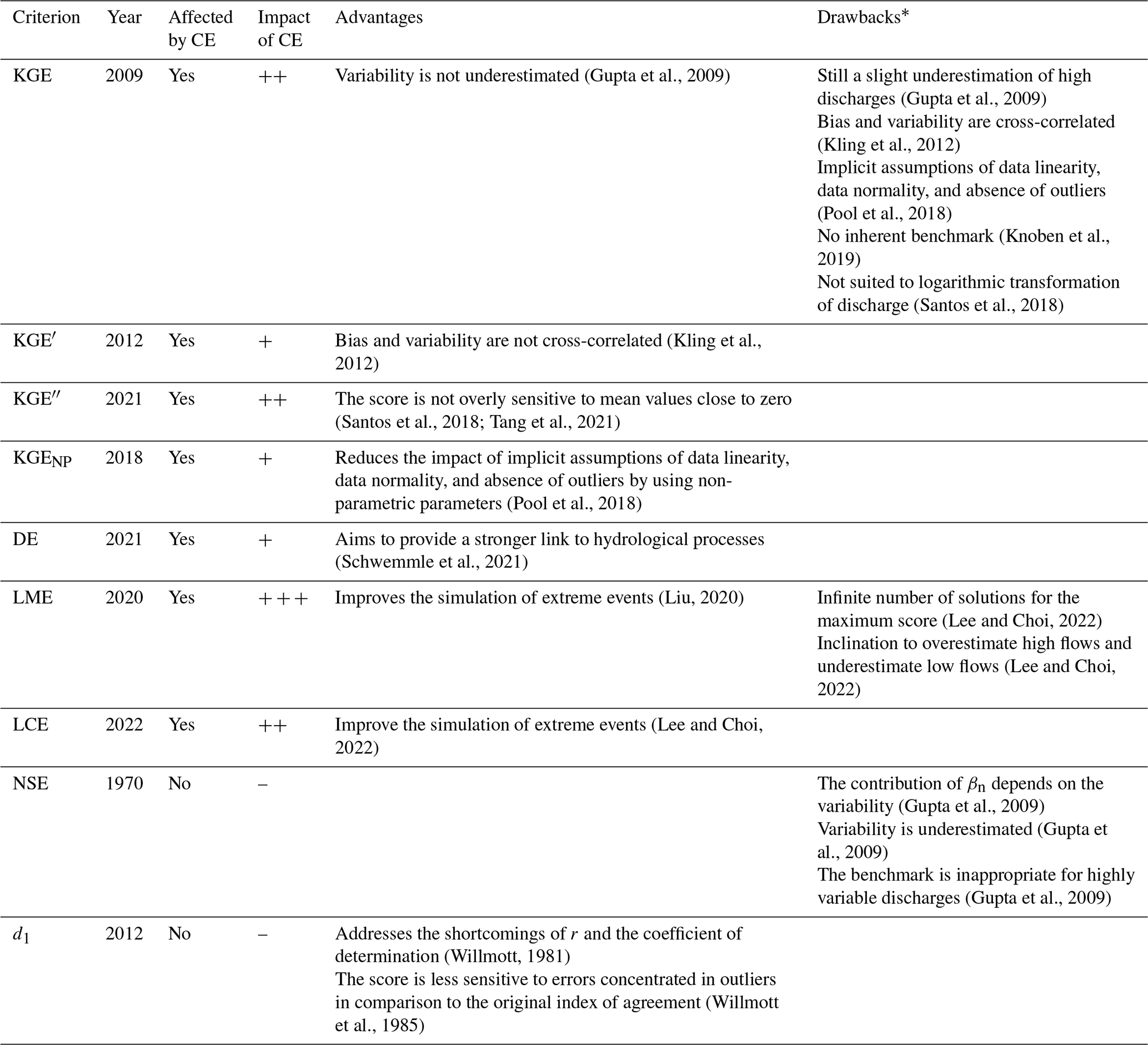
^* KGE drawbacks may likely apply to KGE variants, but this has not been studied extensively.

5.2 Use of scaling factors

The assessment of the hydrological models in the real case study shows how concurrent over- and underestimation can generate counterbalancing errors in bias and variability parameters. For the case study considered in this paper, the ANN model, although offering a better simulation, is evaluated as – sometimes considerably – worse than the bucket-type model because it slightly underestimates the total volume. This has a great impact on the overall score, as the KGE and its variant are calculated with both bias and variability parameters accounting for two-thirds of the overall criterion score.

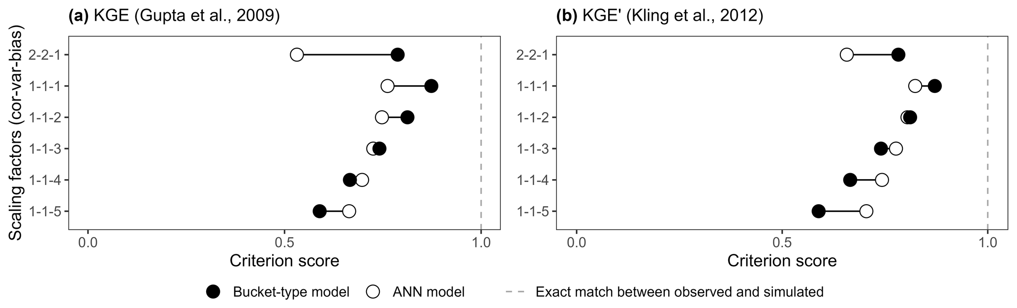
Figure 8 (a) KGE and (b) KGE^′ scores of the ANN and bucket-type models (Fig. 6a) according to different scaling factors. The y-axis numbers correspond to the scaling factors of the variability, bias, and timing parameters, with the default being 1–1–1.

While the overall balance (bias) may be a desired feature in a model, we showed that a good value may be accidental and result from counterbalancing errors. The common use of the KGE neglects one of the original proposals, which is to weight the parameters β, α, and r in the equation. Gupta et al. (2009) proposed an alternative equation for adjusting the emphasis on the different aspects of a model:

$$\begin{array}{}\text{(22)}& {\mathrm{KGE}}_{\mathrm{s}}=\mathrm{1}-\sqrt{{\left[s_{\mathit{\alpha }}(\mathit{\alpha }-\mathrm{1})\right]}^{\mathrm{2}}+{\left[s_{\mathit{\beta }}(\mathit{\beta }-\mathrm{1})\right]}^{\mathrm{2}}+{\left[s_{\mathrm{r}}(r-\mathrm{1})\right]}^{\mathrm{2}}},\end{array}$$

with s_r, s_β, and s_α being the scaling factors of r, β, and α, respectively. By default, these factors are equal to 1, which induces a weight of one-third for the parameter in absolute value (r) and two-thirds for the parameters in relative values (β, α). To the best of our knowledge, only Mizukami et al. (2019) ever considered changing the scaling factors when using the KGE. We suggest that one carefully consider such scaling factors for the calibration and the evaluation of hydrological models using the KGE and its variants. Depending on the purpose of the model, they can help to emphasise particular aspects of a model or reduce the influence of relative parameters and counterbalancing errors.

Figure 8 shows how emphasising absolute parameters with scaling factors helps to reduce the influence of counterbalancing errors for the KGE (Fig. 8a) and its most used variant KGE^′ (Fig. 8b). The default value (1–1–1) – corresponding to scaling factors of 1 for α (KGE) or γ (KGE^′), 1 for β, and 1 for r, respectively – is compared to other factor combinations with different ratios between absolute and relative parameters. The 2:1 ratio (2–2–1) increases counterbalancing errors as the emphasis is on the relative parameters, while the 1:2, 1:3, 1:4, and 1:5 ratios decrease counterbalancing errors. The ANN model is evaluated as better with the 1:4 ratio for the KGE and the 1:3 ratio for the KGE^′, highlighting that the KGE^′ is less sensitive to counterbalancing errors. This also shows how the score of a performance criterion and, by extension, its interpretation can be radically different depending on the parameters used in the equation. This is why a multi-criteria framework can strengthen the evaluation of models and reduce the uncertainty associated with the interpretation of individual performance criteria scores.

6 Conclusion

This study sets out to explore the influence of counterbalancing errors and to raise awareness among modellers about the use of performance criteria for calibrating and evaluating hydrological models. A total of nine performance criteria (NSE, KGE, KGE^′, KGE^′′, KGE_NP, DE, LME, LCE, and d₁) are analysed. The investigation of synthetic time series and real hydrological models shows that concurrent over- and underestimation of multiple parts of a discharge time series may favour bias and variability parameters. This especially concerns the bias parameters (β, β_n, and B_rel) as their values are all influenced by counterbalancing errors in both synthetic time series and the real case study. On the other hand, the impact of counterbalancing errors on the variability parameters seems to depend on the time series: only the value of α is influenced in the synthetic time series, while the values of all variability parameters (α, γ, |B_area|, and α_NP) are influenced in the real hydrological models. As bias and variability parameters generally account for two-thirds of the weight in the equation of certain performance criteria, this can lead to an overall higher criterion score without being associated with an increase in model relevance. This is especially concerning for the KGE and its variants as they generally use relative parameters for evaluating bias and variability in hydrological models. These findings highlight the importance of carefully choosing a performance criterion adapted to the purpose of the model. Recommendations also include the use of scaling factors to emphasise different aspects of a hydrological model and to reduce the influence of relative parameters on the overall score of the performance criterion. Further research could explore the appropriate values of scaling factors to be used, depending on the modelling approach and the purpose of the study.

Appendix A: Common and recently developed performance criteria applied to the synthetic time series and the real case study

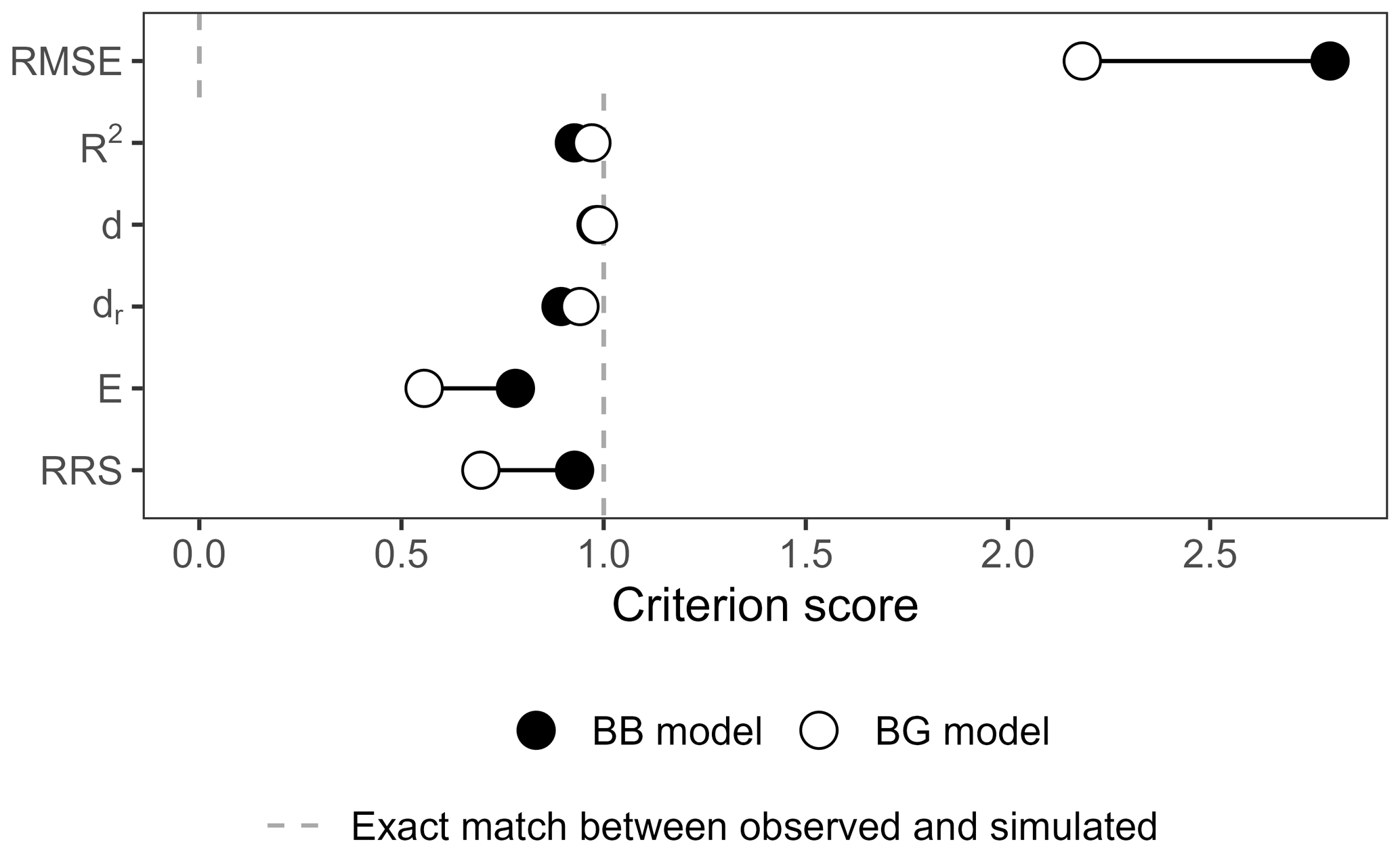
Figure A1 Score of the BB and BG transformations according to other common and recently developed performance criteria: the root mean square error (RMSE), the coefficient of determination R², the index of agreement d (Willmott, 1981), the refined index of agreement d_r (Willmott et al., 2012), the Onyutha efficiency E, and the revised R² (RRS) (Onyutha, 2022).

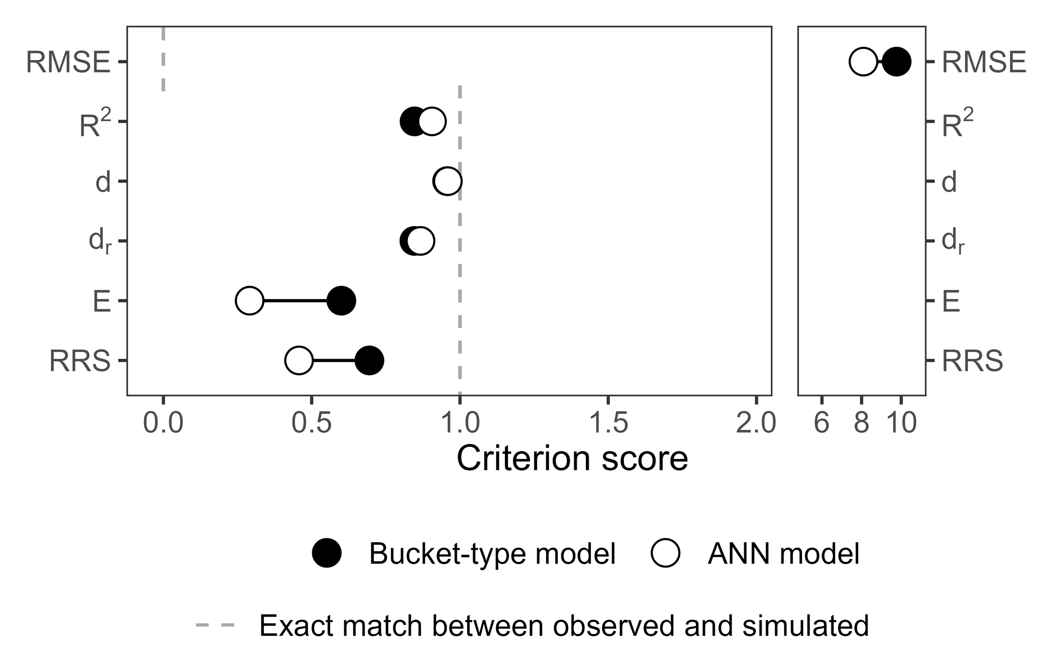
Figure A2 Score of the ANN and bucket-type models according to other common and recently developed performance criteria: the root mean square error (RMSE), the coefficient of determination R², the index of agreement d_r (Willmott, 1981), the refined index of agreement d_r (Willmott et al., 2012), the Onyutha efficiency E, and the RRS (Onyutha, 2022).