Regional significance of historical trends and step changes in Australian streamflow

The Hydrologic Reference Stations is a network of 467 high-quality streamflow gauging stations across Australia that is developed and maintained by the Bureau of Meteorology as part of an ongoing responsibility under the Water Act 2007. The main objectives of the service are to observe and detect climate-driven changes in observed streamflow and to provide a quality-controlled dataset for research. We investigate trends and step changes in streamflow across Australia in data from all 467 streamflow gauging stations. Data from 30 to 69 years in duration ending in February 2019 were examined. We analysed data in terms of water-year totals and for the four seasons. The commencement of the water year varies across the country – mainly from February–March in the south to September–October in the north. We summarized our findings for each of the 12 drainage divisions defined by Australian Hydrological Geospatial Fabric (Geofabric) and for continental Australia as a whole. We used statistical tests to detect and analyse linear and step changes in seasonal and annual streamflow. Monotonic trends were detected using modified Mann–Kendall (MK) tests, including a variance correction approach (MK3), a block bootstrap approach (MK3bs) and a long-term persistence approach (MK4). A nonparametric Pettitt test was used for step-change detection and identification. The regional significance of these changes at the drainage division scale was analysed and synthesized using a Walker test. The Murray–Darling Basin, home to Australia's largest river system, showed statistically significant decreasing trends for the region with respect to the annual total and all four seasons. Drainage divisions in New South Wales, Victoria and Tasmania showed significant annual and seasonal decreasing trends. Similar results were found in south-western Western Australia, South Australia and north-eastern Queensland. There was no significant spatial pattern observed in central nor mid-west Western Australia, with one possible explanation for this being the sparse density of streamflow stations and/or the length of the datasets available. Only the Tanami–Timor Sea Coast drainage division in northern Australia showed increasing trends and step changes in annual and seasonal streamflow that were regionally significant. Most of the step changes occurred during 1970–1999. In the south-eastern part of Australia, the majority of the step changes occurred in the 1990s, before the onset of the “Millennium Drought”. Long-term monotonic trends in observed streamflow and its regional significance are consistent with observed changes in climate experienced across Australia. The findings of this study will assist water managers with long-term infrastructure planning and management of water resources under climate variability and change across Australia.

1 Introduction

Australia is the driest inhabited continent on Earth, receiving only 450 mm yr⁻¹ of rainfall on average (BoM and CSIRO, 2020). Rainfall amounts vary significantly across the country, with approximately 70 % of the landmass being arid or semi-arid and receiving less than 350 mm yr⁻¹ (BOM, 2022). The distribution and amount of rainfall across the country has influenced patterns of human settlement for more than 60 000 years (Williams, 2013). The continent also has unique topographic and geologic features. The central region is mostly arid or semi-arid, the south-eastern and south-western corners have a temperate climate, and the north has a tropical climate (Stern et al., 2000). The eastern and south-eastern coastal regions have mountain ranges. Rainfall is higher and more reliable in coastal regions, except in the mid-western coastal regions of Western Australia. Elevation is another factor that has an important influence on rainfall, with mountainous areas such as north-eastern Queensland, south-eastern Australia and western Tasmania receiving higher rainfall (Holper, 2011). Rainfall is highly variable in both space and time compared with other continents. Together, the unique topographic and geological features and the distribution of rainfall result in great interannual variability in streamflow (Nicholls et al., 1997; Poff et al., 2006), floods and droughts.

The “Millennium Drought” between 1997 and 2009 is described as the worst drought on record for south-eastern Australia (Van Dijk et al., 2013). During 2001–2009, south-eastern Australia suffered the driest period since 1900 – the longest uninterrupted series of years with below-median rainfall (Bureau of Meteorology data; http://www.bom.gov.au/cgi-bin/climate/change/timeseries.cgi, last access: 3 January 2023). Discharge of the Murray River system during this period was half the previous recorded minimum. As a response to the widespread social, financial and environmental impacts of drought, the federal government passed the Water Act 2007 (https://www.legislation.gov.au/Details/C2017C00151, last access: 3 January 2023) legislation through parliament, heralding the implementation of a water security plan for Australia. One of the important roles in realizing the water security plan is enhancing our understanding of Australia's water resources. The Hydrologic Reference Stations service (http://www.bom.gov.au/water/hrs/index.shtml, last access: 3 January 2023) was developed to provide greater insight into climate-driven changes in streamflow across Australia. Similar services exist in Canada, the United States, Europe (Bradford and Marsh, 2003; Brimley et al., 1999; Coxon et al., 2020; Falcone et al., 2010; Lins, 2012; Whitfield et al., 2012) and other areas across the globe (Alfieri et al., 2020). In Canada, spatial and temporal trends in streamflow and other associated hydroclimatic variables show increasing and decreasing patterns in northern and mid-latitude catchments respectively (Bawden et al., 2015; O'Neil et al., 2017). In the continental United States, streamflow analyses from 1940 to 2009 for 967 gauging stations show overall decreasing trends, including higher annual maxima and lower annual minima (Rice et al., 2015). Similar results were also reported by Asadieh et al. (2016) for the 1971–2001 period in the United States and other continents across the world. When comparing trends in minimally altered or regulated catchments in the United States, Hodgkins et al. (2020) found that there were larger changes in median streamflow compared with changes in annual 1 d high or 7 d low flows. Shifts in flood peaks and streamflow timing were found to be consistent with changes in rainfall, in both natural and managed catchments (Ficklin et al., 2018). In Finland, trend analysis revealed no changes in mean annual flow overall, but some changes in the seasonal distribution of streamflow were found (Korhonen and Kuusisto, 2010). In south-eastern Asia and Africa, analyses of observed streamflow mostly show downward trends. In the Senegal River basin, analysis of annual streamflow showed decreasing trends (Diop et al., 2018), whereas dry-season flows increased by 6 % in the Black Volta basin in West Africa over the period from 2000 to 2013 (Akpoti et al., 2016). Decreasing trends were also found in streamflow extremes across China (Li et al., 2020) as well as in streamflow in the Huaihe River basin, China (Pan et al., 2018). Similar trends were also evident in annual streamflow in West Borneo, Indonesia (Herawati and Suharyanto, 2015).

Global-scale investigation of trends in annual maximum streamflow has revealed that decreasing trends tend to occur in Asia, Australia, the Mediterranean, the western and north-eastern United States, and northern Brazil and that increasing trends appear mostly in central North America, southern Brazil and the northern part of western Europe (Do et al., 2017). Rainfall is one potential driver of these changes. Through analyses of streamflow trends, using data from more than 30 000 gauges across the world, Gudmundsson et al. (2019) found that, where trends are present in a region, the direction of the trend is often consistent across all trend analysis indicators, including high, average and low flows, for that specific region. Analyses of floods and extreme streamflow events across the world show little to suggest that increases in heavy-rainfall events at higher temperatures result in similar increases in streamflow (Wasko and Sharma, 2017). However, shifts in the timing of flood peaks and changes in streamflow timing were found to be consistent with rainfall change and in a similar direction (Wasko et al., 2020).

Australian streams showed the greatest influence of interannual variability in flow (Poff et al., 2006). Chiew and McMahon (1993) examined annual streamflow series of 30 unregulated Australian catchments to detect trends or changes in the means. They concluded that any changes were directly related to interannual variability, rather than to any changes in climate. Analysis of trends in Australian flood data from 491 stations (Ishak et al., 2010) indicated that about 30 % showed trends in the annual maximum flood, with downward and upward trends in southern and northern parts of Australia respectively. Analyses of 780 unregulated catchments (Gu et al., 2020) revealed a similar geographical distribution of trends. Other studies have investigated trends in selected streamflow components in particular regions, such as the south-western region of Western Australia (Durrant and Byleveld, 2009; Petrone et al., 2010) and south-eastern Victoria (Tran and Ng, 2009). In Victoria and the Australian Alps, the assessment and reconstruction of catchment variability and trends in streamflow showed a decline during the period from 1977 to 2012 (Fiddes and Timbal, 2016). A similar spatial pattern in streamflow reduction also occurred during the Millennium Drought between 1997 and 2009. Johnson et al. (2016) reviewed historical trends and variability in flood events across Australia and concluded that the link between trends in flood events and rainfall cannot be made due to the influence of climate processes, such as temperature and evapotranspiration, over different spatial and temporal scales. Similar results were also reported by Wasko and Nathan (2019) and Sharma et al. (2018): changes in rainfall and soil moisture did not always explain trends in flooding.

The studies above undertook trend analysis of Australian rivers with limited spatial or temporal coverage of streamflow data. This study undertakes a systematic appraisal of changes and trends in observed streamflow records in a large number of catchments across the country which are largely unaffected by human influence. Zhang et al. (2016) undertook the first comprehensive study employing the Hydrologic Reference Stations and analysed data until 2014 from 222 stations across Australia. That study investigated many components of streamflow (including annual total, high and low flows; seasonal totals; and baseflow components); these components were analysed and are presented at http://www.bom.gov.au/water/hrs (last access: 3 January 2023). The above study considered only the streamflow variables that are random and did not consider the effect of the autocorrelation structure and long-term persistence on the trend in streamflow variables. The Hydrologic Reference Stations service is now updated and contains information for 467 gauging stations and streamflow data until February 2019. In this study, we focus on monotonic trends and step changes in annual and seasonal streamflow across different drainage divisions of Australia as well as their regional significance. The investigation of changes in other streamflow variables or the driving forces of changes in rainfall patterns on these resulting trends in streamflow is outside the scope of this study. Results from this study will benefit managers and researchers in sustainable water management and long-term planning in water allocation, agricultural planning and hydropower.

2 Selection of gauging stations and data quality

2.1 Station selection guidelines

Guidelines for the selection of the Hydrologic Reference Stations (HRS) were described in detail by Turner (2012). These include a minimum of 30 years of continuous data with less than 5 % of missing data in unimpaired catchments. Details of the station selection procedure are provided on the HRS website. In a recent update of the service, the Bureau of Meteorology implemented two additional criteria: (i) the percentage of flow volume included as infilled data and (ii) the percentage of flow volume above the maximum gauged discharge. The thresholds for these two criteria were (i) a maximum of 10 % for flow volume of infilled data and (ii) a restriction of extrapolated data to a maximum of 25 %. Details of the station selection guidelines are presented on the website. All 467 gauging stations that met these guidelines and were included in the updated service are included in this study.

2.2 Updated number of gauging stations

2.2.1 Gauging stations in the 2020 update

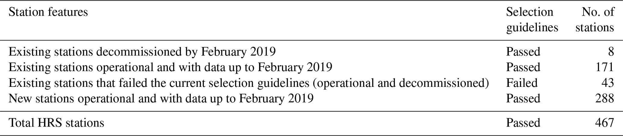
Of the existing 222 gauging stations in the network prior to the service (Zhang et al., 2016), 12 have now been decommissioned by the data-provision agencies, including 5 from the Northern Territory, 2 from Victoria, 2 from Western Australia, 1 from New South Wales and 2 from South Australia. The revised and updated selection guidelines were applied to all 222 gauging stations, and 179 of these stations passed the new guidelines. More information about the rating curves of 43 existing stations became available and suggested that these stations did not pass the selection criteria. Therefore, these 43 stations were removed from the HRS service in 2020 (Table 1).

Table 1 Total number of stations.

2.2.2 New stations included in the service

Australia's instrumental record is relatively sparse before 1940, and few locations have continuous rainfall measurement before 1900. At present, there are approximately 4800 streamflow gauging stations across Australia. Many of these stations previously had insufficient data in the Bureau's system to be considered for the HRS service. Over recent years, more data have become available, and a set of 780 stations identified by Zhang et al. (2013) were selected for further investigation. These 780 unregulated, unimpaired catchments are widely spread across Australia (Fig. 1) and have undergone strict quality assurance/quality control (QA/QC), including quality code checking for daily streamflow records (Zhang et al., 2013). The total number of streamflow gauging stations that met the new guidelines and are now included in the service is 467, which is an increase from 222 stations (Table 1).

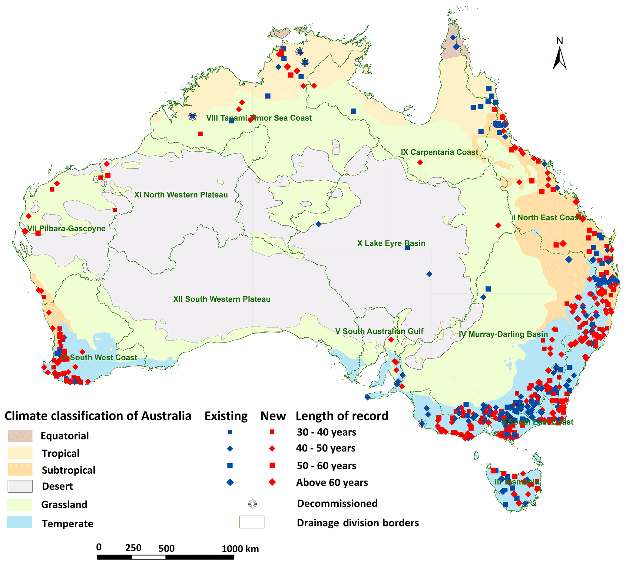
Figure 1 Map of Australia showing climate zones, drainage divisions and the location of all gauges (new, existing and decommissioned), all scaled to length of record.

2.2.3 Reference period, quality control and catchment description

The HRS service was updated with streamflow data ending in February 2019. This month was chosen to capture the 2018 water year for all stations. Commencement of recording of streamflow data varies across the country. The longest record begins in the 1950s and the shortest begins in the 1980s. Figure 1 shows the location of stations and the duration of the records, including the eight decommissioned stations. Data recorded at stations prior to 1950 were excluded from analysis, as the missing data were more than 5 % before this time in most cases. Stations with the longest records are generally those in the high-value water resource catchments and populated areas along the coastal regions. Upstream catchment area also varied across the country (from 4.5 to 232 846 km²) and in different hydroclimatic regions (Table 2). Most of the catchment areas ranged from 50 to 10 000 km² (Table 2). The number of stations distributed across different drainage divisions varies substantially: the Murray–Darling division has the largest number of stations, whereas the South Western Plateau division has no stations at all. Drainage divisions are defined according to Australian Hydrological Geospatial Fabric (Geofabric) (Atkinson et al., 2008). In a previous update of the HRS service (Zhang et al., 2016), there were no stations in the Pilbara–Gascoyne and North Western Plateau divisions. In the current version, there are 10 and 2 stations in these divisions respectively (Fig. 1, Table 2).

Table 2 Metadata for drainage divisions and selected hydrologic reference stations.

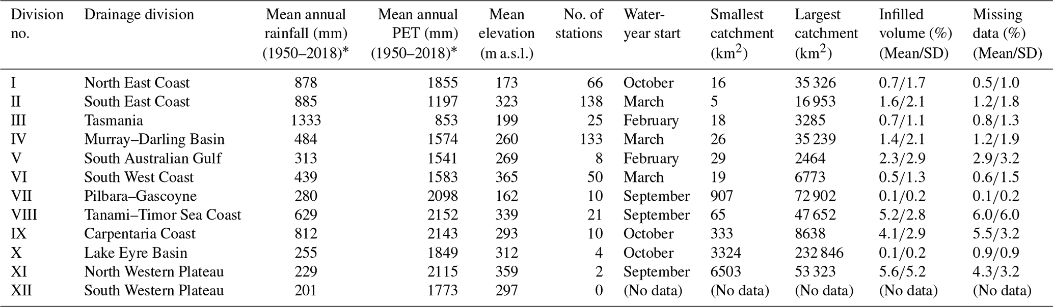
^* Calculated from monthly gridded rainfall and potential evapotranspiration (PET) data (5 km × 5 km) from the Australian Water Availability Project – AWAP (Raupach et al., 2009).

Continental Australia has a wide range of climate zones, as defined by Köppen climate classification (Stern et al., 2000), including a tropical region in the north, temperate regions in the south, and grassland and desert in the vast interior (Fig. 1). In this work, water year is defined in accordance with the Hydrologic Reference Stations' glossary (http://www.bom.gov.au/water/hrs/glossary.shtml, last access: 3 January 2023). It varies across the country – beginning in February–March in the south and in September–October in the north (Table 2). Annual average rainfall for each of the divisions varies from 201 to 1333 mm. Annual average potential evapotranspiration (PET) is generally higher than the annual average rainfall. Therefore, the streamflow generation process in most of the divisions is controlled by water-limited environments (Milly et al., 2005) except for the Tasmanian division (Table 2). Figure 2a shows the relationship between the catchment area and record length. Figure 2b, in contrast, shows the relationship between the catchment area and the distribution of the percentage of catchments: the distribution is reasonably uniformly distributed in the range between 45 and 12 000 km² and is slightly skewed outside of this range. The longest period of record is 69 years for several catchments with an area from 14 to 15 850 km².

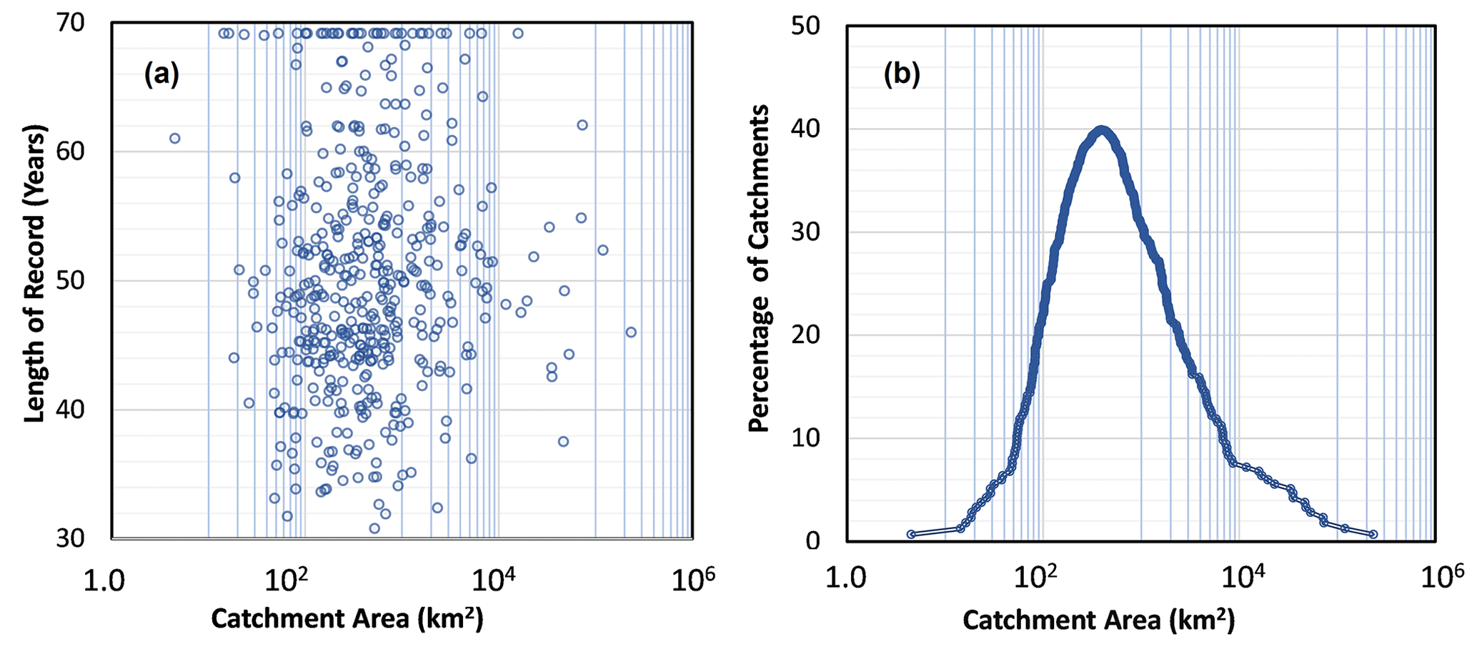
Figure 2 Catchment area plotted against (a) the length of record and (b) the percentage of catchments.

A QA/QC process was applied to observed time series of daily streamflow from each gauging station. This process identified and removed erroneous data values such as negative and extreme values. The process of detection and removal was automated and then checked manually, as detailed on the Hydrologic Reference Stations website (http://www.bom.gov.au/water/hrs/references.shtml, last access: 3 January 2023). The GR4J model (Perrin et al., 2003) was adopted to infill any missing data in accordance with the selection guidelines detailed in Sect. 2.1. The mean and standard deviation of the Nash–Sutcliffe efficiency for all 467 catchments was 0.74 and 0.12 respectively. As part of this process, a simple error correction procedure was used to ensure that the initial and final estimated flows matched adjacent observed values. This was done by linearly interpolating the start and end of the infilled period to the observed flows. Via this process, a continuous quality-checked daily streamflow time series was created for trend analyses.

3 Methodology

Quality-controlled and infilled daily data were accumulated to annual totals (based on water year) and to the total for each of the four seasons. These five streamflow statistics formed the basis for trend analysis to capture annual and seasonal trends. Seasons are defined as winter (June–August), spring (September–November), summer (December–February) and autumn (March–May).

There are generally two types of change often observed in streamflow datasets: long-term persistent trends (monotonic change) and sudden abrupt change (step change). Monotonic trends generally occur due to long-term changes in rainfall, temperature and/or evapotranspiration, whereas step changes generally result from sudden changes in flow generation thresholds. Statistical tests used to detect monotonic trends and step changes in streamflow generally fall into two categories: parametric and nonparametric tests.

3.1 Trend analyses

We applied the Theil–Sen approach (Sen, 1968; Theil, 1992), a nonparametric technique, to detect the magnitude of the linear trend for each of the statistics (the annual total and the four seasons' totals). In addition, trends were determined using the nonparametric Mann–Kendall (MK) test (Kendall, 1975; Mann, 1945), as this technique is distribution-free, robust against outliers and has a higher power for non-normally distributed data (Önöz and Bayazit, 2003; Yue et al., 2002). It has also been commonly used in streamflow trend analyses (Abdul Aziz and Burn, 2006; Birsan et al., 2005; Dixon et al., 2006; Lins and Slack, 1999). The MK test requires input data to be serially uncorrelated; any serial correlation in the data structure can lead to an overestimation of the significance of trends (Hamed and Ramachandra Rao, 1998; von Storch, 1995; Yue et al., 2002). To overcome the effect of serial correlation of higher order (namely short-term persistence – STP), two techniques are used here: (i) a modified MK test, commonly known as the variance correction (MK3) method (as proposed by Hamed and Ramachandra Rao, 1998), and (ii) a block bootstrap (MK3bs) method (Kundzewicz and Robson, 2000). The MK3 and MK3bs approaches are more suitable when the time series shows higher-order serial dependencies. Apart from short-term persistence (STP), the presence of long-term persistence (LTP), or the Hurst phenomenon, has been identified as a major source of uncertainty when analysing hydroclimatic data series (Koutsoyiannis, 2003; Kumar et al., 2009). To incorporate LTP behaviour in the MK test, the technique proposed by Hamed (2008) is used in this study. Employing these three modified versions of the MK test allows for a comparison of differences and also allows the validity of results for Australia to be checked. A nonparametric Pettitt test (Pettitt, 1979) and distribution-free CUSUM (cumulative sum) test (Chiew and Siriwardena, 2005) are generally used to detect abrupt step changes in streamflow. A Pettitt test was used to detect step change for all five streamflow statistics, as it performs better than others with respect to detecting step change and identifying the change point (Villarini et al., 2009). Finally, the regional significance of any monotonic trends and step changes was tested using a Walker test (Wilks, 2006).

The Theil–Sen slope approach, the original Mann–Kendall (MK) test, three modified versions of the MK test, the Pettitt test and the Walker test are briefly described in this section. Trend detection analysis may lead to misleading results when serial correlation (STP) and long-term persistence (LTP) in the streamflow data are ignored. The modified versions of the Mann–Kendall test, MK3, MK3bs and MK4, which account for STP, STP and LTP respectively, are used to identify trends in streamflow data. A more detailed description can be found in Mann (1945), Kendall (1975), Hamed and Ramachandra Rao (1998), Koutsoyiannis (2003) Hamed (2008), Pettitt (1979), Wilks (2006), Kumar et al. (2009), Zamani et al. (2017), Su et al. (2018), and Kundzewicz and Robson (2000).

We used the Theil–Sen estimator and three different forms of the Mann–Kendall test, (i) a variance correction approach, (ii) a block bootstrap approach and (iii) long-term persistence, for monotonic trend analyses.

3.1.1 The Theil–Sen approach

The magnitude of the trend is obtained using the Theil–Sen approach (Theil, 1992; Sen, 1968), where the magnitude of the slope of the trend is estimated as follows:

$$\begin{array}{}\text{(1)}& \mathit{\beta }=\mathrm{median}\left[\left(x_i-x_j\right)(i-j)\right];\mathrm{for}\mathrm{all}j<i.\end{array}$$

Here, x_i and x_j are streamflow data (annual and all seasons) at time points i and j respectively. If the time series has n values, there will be $N=n(n-\mathrm{1})/\mathrm{2}$ slope estimates, and the Theil–Sen slope β is taken as the median of these N values.

3.1.2 Independent Mann–Kendall (MK1) test

The Mann–Kendall test statistic (S) for a series x₁, x₂, x₃, …, x_n is given by

$$\begin{array}{}\text{(2)}& S=\sum _{i=\mathrm{1}}^{n-\mathrm{1}}\sum _{j=i+\mathrm{1}}^n\mathrm{sgn}\left(x_j-x_i\right),\end{array}$$

where

$$\begin{array}{}\text{(3)}& \mathrm{sgn}\left(\mathit{\theta }\right)=\left\{\begin{array}{ll}\mathrm{1}& \mathrm{if}\mathit{\theta }>\mathrm{0}\\ \mathrm{0}& \mathrm{if}\mathit{\theta }=\mathrm{0}\\ -\mathrm{1}& \mathrm{if}\mathit{\theta }<\mathrm{0}.\end{array}\right.\end{array}$$

The test statistic S is approximately normally distributed for n≥8 with zero mean. The variance as given as follows:

$$\begin{array}{}\text{(4)}& V\left(S\right)=\left[n(n-)(\mathrm{2}n+\mathrm{5})-\sum _{i=\mathrm{1}}^m\left(t_i-\mathrm{1}\right)\left(\mathrm{2}{t}_i+\mathrm{5}\right)t_i\right]/\mathrm{18},\end{array}$$

where m is the number of tied groups, and t_i is the number of data in the ith tied group. The standardized test statistic Z (standard normal distribution) is given as follows:

$$\begin{array}{}\text{(5a)}& {\displaystyle }& {\displaystyle }Z={\displaystyle \frac{(S-\mathrm{1})}{\sqrt{V\left(S\right)}}}\mathrm{if}S>\mathrm{0}\text{(5b)}& {\displaystyle }& {\displaystyle }Z=\mathrm{0}\mathrm{if}S=\mathrm{0}\text{(5c)}& {\displaystyle }& {\displaystyle }Z={\displaystyle \frac{(S+\mathrm{1})}{\sqrt{V\left(S\right)}}}\mathrm{if}S<\mathrm{0}.\end{array}$$

To identify and address the short-term and long-term persistence in a streamflow series, we used three modified versions the of Mann–Kendall test for monotonic trend analyses: (i) the variance correction approach, (ii) the block bootstrap approach and (iii) the long-term persistence approach.

3.1.3 Mann–Kendall (MK3) test – variance correction approach

The modified Mann–Kendall variance correction approach, proposed by Hamed and Ramachandra Rao (1998), considers all of the significant autocorrelation structure in a time series. The series x_i was ranked, and an autocorrelation coefficient of rank i of time series was obtained to consider only the significant terms at the 10 % significance level. Autocorrelation becomes insignificant after a lag of 3 (Rao et al., 2003). The effect of all significant autocorrelation coefficients in the dataset was removed using a modified variance of S, described as V(S)^*:

$$\begin{array}{}\text{(6)}& V(S{)}^{*}=V(S){\displaystyle \frac{n}{n^{*}}},\end{array}$$

where n^* represents the effective sample size. The $\frac{n}{n^{*}}$ ratio was computed directly from the equation proposed by Hamed and Ramachandra Rao (1998) as follows:

$$\begin{array}{}\text{(7)}& {\displaystyle \frac{n}{n^{*}}}=\mathrm{1}+{\displaystyle \frac{\mathrm{2}}{n(n-\mathrm{1})(n-\mathrm{2})}}\sum _{i=\mathrm{1}}^{n-\mathrm{1}}(n-i)(n-i-\mathrm{1})(n-i-\mathrm{2})r_i,\end{array}$$

where n is the number of observations, and r_i is the lag-i significant autocorrelation coefficient of rank i of time series. V(S)^* is calculated using Eq. (6) and using V(S) from Eq. (4). Finally, the Mann–Kendall Z was tested for significance of trend by comparing it with threshold levels.

3.1.4 Mann–Kendall (MK3bs) test – block bootstrap (BBS) approach

The block bootstrap (BBS) approach by Önöz and Bayazit (2003) was used to mitigate the effects of serial correlation in datasets by performing bootstrapping (in blocks of data) so that the autocorrelation in the data is replicated. Data are resampled in blocks many times to estimate the significance of the observed Mann–Kendall test statistic S from the data sample while reflecting the serial correlation present in the dataset (Burn et al., 2016). Block length should be chosen so that data points in adjacent block are more or less independent. Khaliq et al. (2009) provide a detailed description of the steps involved in implementing the BBS approach.

In block bootstrapping, the simulation size N_s (the number of bootstrap samples to be generated in each case) and the block length L_b are the parameters whose values are to be chosen. The simulation size (N_s) is related to the level of significance required and the loss of power that can be allowed. Svensson et al. (2005) found that N_s=2000 samples resulted in good stability in significance level estimates. The block length chosen depends on autocorrelation of the data and should be larger than the lag k of the smallest significant autocorrelation coefficient R_i. Svensson et al. (2005) found that blocks with lengths of 5 were generally sufficient for most streamflow series.

Autocorrelation in time series varies across different sites, and Politis (2003) recommends that the block length L_b is based on individual time series. To identify the optimal block length (L_b) for individual annual and seasonal streamflow time series, an automatic block length selection procedure, proposed by Politis and White (2004), was used. The optimal block lengths obtained for the annual streamflow time series and for each of the four seasonal streamflow time series for 467 gauging stations are shown in Fig. 3. In general, more than one-third of the stations exhibit significant serial correlation of 2 or more (L_b≥3), and about 15 % of the stations are serially uncorrelated (L_b=1).

Figure 3 The optimal block length for the annual streamflow time series and the four seasonal streamflow time series for all 467 stations.

We estimated the significance of the original Mann–Kendall test statistic S (Eq. 2) of the observed data from the simulated distribution, developed from the resampled distribution of S from the moving block bootstrap procedure. The test statistic is only likely to be significant if the original test statistic lies within the tails of the simulated distribution (Do et al., 2017; Khaliq et al., 2009).

3.1.5 Mann–Kendall (MK4) test – long-term persistence (LTP)

The long-term persistence (LTP) version of the Mann–Kendall method was proposed by Hamed (2008) and described by Kumar et al. (2009), and it considers the Hurst coefficient (Hurst, 1951), H, of a series for LTP. The coefficient H is used as a measure of long-term memory, i.e. autocorrelation of the time series. An H value of 0.5 indicates a true random walk, which implies that the time series has no memory for previous values of observations. An H value between 0.5 (0) and 1 (0.5) indicates a time series with positive (negative) autocorrelation, e.g. an increase (decrease) between observations will probably followed by another increase (decrease).

In this study, the following steps were carried out to apply the MK4 test:

1. The Hurst coefficient (H) is calculated. A new trend-free time series $x_i^{\prime }$ is calculated using

   $$\begin{array}{}\text{(8)}& x_i^{\prime }=x_i-(\mathit{\beta }\times i),\end{array}$$

   where β is the slope of a trend line using the Theil–Sen approach, and x_i is the streamflow data. Using the ranks of trend-free series [$x_i^{\prime }:(i=\mathrm{1}:n)$] designated by R_i, the standardized Z_i variate (the equivalent normal variates of the ranks of detrended time series) is computed as

   $$\begin{array}{}\text{(9)}& Z_i={\mathit{\phi }}^{-\mathrm{1}}\left({\displaystyle \frac{R_i}{n+\mathrm{1}}}\right),\end{array}$$

   where n is the number of streamflow data, and φ⁻¹ is the inverse of the normal distribution function. Considering the hypothesis that the hydrometeorological processes exhibit scale-invariant properties at any scale greater than annual (Koutsoyiannis, 2003), the elements of the Hurst matrix for a given H are computed as

   $$\begin{array}{}\text{(10)}& {\mathbf{C}}_{\mathrm{n}}\left(H\right)=⌊{\mathit{\rho }}_{|j-i|}\left(H\right)⌋\mathrm{for}i=\mathrm{1}:n,j=\mathrm{1}:n.\end{array}$$

   In the above equation, ρ_l(H) is the lag-l autocorrelation coefficient for a given H and is calculated as

   $$\begin{array}{}\text{(11)}& {\mathit{\rho }}_l\left(H\right)={\displaystyle \frac{\mathrm{1}}{\mathrm{2}}}\left(|l+\mathrm{1}{|}^{\mathrm{2}H}-\mathrm{2}{l}^{\mathrm{2}H}+|l-\mathrm{1}{|}^{\mathrm{2}H}\right)\mathrm{for}l>\mathrm{0}.\end{array}$$

   The log-likelihood function of n normal observations with a scaling coefficient H is given by Eq. (12) (McLeod and Hipel, 1978), where the accurate value of H can be computed by maximizing the function of H as

   $$\begin{array}{}\text{(12)}& \log L\left(H\right)=-{\displaystyle \frac{\mathrm{1}}{\mathrm{2}}}\log \mathrm{|}{\mathbf{C}}_n\left(H\right)\mathrm{|}-{\displaystyle \frac{Z^{\mathrm{T}}\mathrm{|}{\mathbf{C}}_n\left(H\right){\mathrm{|}}^{-\mathrm{1}}\mathit{Z}}{\mathrm{2}{\mathit{\gamma }}_{\mathrm{0}}}}.\end{array}$$

   In the above equation, Z^T is the transpose of vector Z obtained from Eq. (9), γ₀ equates the variance of Z_i, and C_n(H) and C_n(H)⁻¹ are the Hurst matrix and the inverse of the Hurst matrix respectively. These two last matrices can be obtained using Eq. (10). To maximize log L(H), H is assumed to be in the range of 0.5–0.98, and the mentioned function is computed for a given H. The procedure is repeated for other H values with 0.01 steps. The H value producing the maximum value of log L(H) is taken as the answer.

2. The mean and standard deviation of H are calculated. According to Hamed (2008), the respective mean and standard deviation of H are expressed as a function of n as

   $$\begin{array}{}\text{(13)}& {\displaystyle }& {\displaystyle }{\mathit{\mu }}_{\mathrm{H}}=\mathrm{0.5}-\mathrm{2.87}{n}^{-\mathrm{0.9067}},\text{and}\text{(14)}& {\displaystyle }& {\displaystyle }{\mathit{\sigma }}_{\mathrm{H}}=\mathrm{0.77654}{n}^{-\mathrm{0.5}}-\mathrm{0.0062}.\end{array}$$

   Z_cal is then calculated as

   $$\begin{array}{}\text{(15)}& Z_{\mathrm{cal}}={\displaystyle \frac{H-{\mathit{\mu }}_{\mathrm{H}}}{{\mathit{\sigma }}_{\mathrm{H}}}}.\end{array}$$

   This Z_cal, obtained from Eq. (15), was tested for significance of trend at the 10 % significance level. The MK4 procedure was continued if Z_cal was greater than the critical normal value (1.645); otherwise, the procedure for an independent Mann–Kendall (MK1) test was adapted as the LTP was not significant.

3. Significant H values are computed (LTP is significant). The modified variance for the S statistic was computed as recommended by Kumar et al. (2009) and Hamed (2009). This took the form of

   $$\begin{array}{}\text{(16)}& \begin{array}{rl}V(S{)}^{H^{\prime }}=& \sum _{i=\mathrm{1}}^{n-\mathrm{1}}\sum _{j=i+\mathrm{1}}^n\sum _{k=\mathrm{1}}^{n-\mathrm{1}}\sum _{l=k+\mathrm{1}}^n{\displaystyle \frac{\mathrm{2}}{\mathit{\pi }}}{\sin }^{-\mathrm{1}}\\ & \left({\displaystyle \frac{\mathit{\rho }|j-l|-\mathit{\rho }|i-l|-\mathit{\rho }|j-k|+\mathit{\rho }|i-k|}{\sqrt{(\mathrm{2}-\mathrm{2}\mathit{\rho }|i-j\left|\right)(\mathrm{2}-\mathrm{2}\mathit{\rho }|k-l\left|\right)}}}\right).\end{array}\end{array}$$

   In the above equation, ρ_l is calculated using Eq. (11) for a given value of H. As $V(S{)}^{H^{\prime }}$ is a biased estimator, we have corrected it for bias using

   $$\begin{array}{}\text{(17)}& V(S{)}^H=V(S{)}^{H^{\prime }}\times B,\end{array}$$

   where B is expressed as a function of sample size, n (Hamed, 2008; Kumar et al., 2009).

   $$\begin{array}{}\text{(18)}& B=a_{\mathrm{0}}+a_{\mathrm{1}}H+a_{\mathrm{2}}{H}^{\mathrm{2}}+a_{\mathrm{3}}{H}^{\mathrm{3}}+a_{\mathrm{4}}{H}^{\mathrm{4}}\end{array}$$
   $$\begin{array}{}\text{(19a)}& {\displaystyle }& {\displaystyle }{a}_{\mathrm{0}}={\displaystyle \frac{\mathrm{1.0024}n-\mathrm{2.5681}}{n+\mathrm{18.6693}}}\text{(19b)}& {\displaystyle }& {\displaystyle }{a}_{\mathrm{1}}={\displaystyle \frac{-\mathrm{2.2510}n+\mathrm{157.2075}}{n+\mathrm{9.2245}}}\text{(19c)}& {\displaystyle }& {\displaystyle }{a}_{\mathrm{2}}={\displaystyle \frac{\mathrm{15.3402}n-\mathrm{188.6140}}{n+\mathrm{5.8917}}}\text{(19d)}& {\displaystyle }& {\displaystyle }{a}_{\mathrm{3}}={\displaystyle \frac{-\mathrm{31.4258}n+\mathrm{549.8599}}{n-\mathrm{1.1040}}}\text{(19e)}& {\displaystyle }& {\displaystyle }{a}_{\mathrm{4}}={\displaystyle \frac{\mathrm{20.7988}n-\mathrm{419.0402}}{n-\mathrm{1.9248}}}\end{array}$$

   When using the MK4 method, V(S)^H obtained from Eq. (17) was used as V(S) in Eq. (5) of the MK1. The significance of Z was then tested for significance of a trend.

3.2 Pettitt test for step change

We used the nonparametric Pettitt test (PT; Pettitt, 1979) to detect step changes in annual and seasonal streamflow. This procedure is least sensitive to outliers and to skewed distributions of the streamflow datasets, in comparison with other methods used for detecting step changes, which makes it most suitable for this analysis (Sagarika et al., 2014). This test can identify anomalies in the mean and/or median streamflow when the time of step change is unclear. It uses a version of the Mann–Whitney statistics to quantify the significance of probabilities by testing two samples from the same population. In the Pettitt test, the p value is computed in a manner that adjusts for the fact that the method is designed to find the most advantageous point in the record to consider as the change point (Helsel et al., 2020; Villarini et al., 2009).

Using Pettitt (1979), let us assume n to be the length of the time series and τ to be the year of the step change. Viewing the time series as two samples x₁, …, x_τand x_τ+1, …, x_n, an index, V_τ can be defined as follows:

$$\begin{array}{}\text{(20)}& V_{\mathit{\tau }}=\sum _{j=\mathrm{1}}^n\mathrm{sgn}\left(x_{\mathit{\tau }}-x_j\right),\end{array}$$

where sgn(x) is the same as sgn(θ) in Eq. (3), and U_τ is defined in Eq. (21).

$$\begin{array}{}\text{(21)}& U_{\mathit{\tau }}=\sum _{i=\mathrm{0}}^{\mathit{\tau }}{V}_i\end{array}$$

When a significant step change exists in a time series, a graph between |U_τ| and τ increases up to the step-change point and then decreases again, or vice versa. However, in the absence of a step-change point, the graph would continually increase or decrease to the end of the time series. The most significant step-change point τ is established at the point where |U_τ| is maximum, given as K_n and defined by

$$\begin{array}{}\text{(22)}& K_n=\begin{array}{c}\max \\ \mathrm{1}\le t\le n\end{array}\mathrm{|}{U}_{\mathit{\tau }}\mathrm{|}.\end{array}$$

In a year where |U_τ| is the maximum, the significance probability associated with K_n is approximated by

$$\begin{array}{}\text{(23)}& p=\mathrm{2}{e}^{\left(\frac{-\mathrm{6}{K}_n^{\mathrm{2}}}{n^{\mathrm{3}}+n^{\mathrm{2}}}\right)}\end{array}$$

where the approximation holds and is accurate to two decimal places, for p<0.5 (Pettitt, 1979).

In this study, we adopted a significance level of p≤0.10 and evaluated the direction of change. The minimum value of U_τ, extracted by K_n, indicates positive change, and a maximum value indicates a negative change.

3.3 Test for regional significance

We assessed the regional significance of trends detected at a local point scale to examine if similar trends were also detected at neighbouring locations. The main objective is to assess whether a certain minimum number of locations with significant trends occur at a regional scale, thereby indicating regional significance, or not. The test for regional significance is rather conservative, as it is based on a null hypothesis of independent trends across stations, when the trends within a region are positively correlated. We applied a Walker test (Wilks, 2006; Sagarika et al., 2014) to detect regional significance of monotonic and step changes in streamflow time series – for the annual total and across the four seasons at a 90 % confidence level (p≤0.10) for all 467 stations across Australia.

The Walker test considers a set of K independent MK and Pettitt tests, all of whose null hypotheses are assumed to be true (i.e. corresponding p values are assumed to be uniformly distributed as U(0, 1)). We further assume that p₍₁₎ is the smallest of the p-value set. In this case, the probability distribution p₍₁₎ is given by

$$\begin{array}{}\text{(24)}& {\displaystyle }& {\displaystyle }f\left[p_{\left(\mathrm{1}\right)}\right]={\displaystyle \frac{K\mathrm{!}}{\left(\mathrm{1}\right)\mathrm{!}(K-\mathrm{1})\mathrm{!}}}{p}_{\left(\mathrm{1}\right)}^{\mathrm{0}}{\left[\mathrm{1}-p_{\left(\mathrm{1}\right)}\right]}^{K-\mathrm{1}}\mathrm{0}\le p_{\left(\mathrm{1}\right)}\le \mathrm{1}\text{(25)}& {\displaystyle }& {\displaystyle }f\left[p_{\left(\mathrm{1}\right)}\right]=K{\left[\mathrm{1}-p_{\left(\mathrm{1}\right)}\right]}^{K-\mathrm{1}}.\end{array}$$

To reject the global null hypothesis that all K local null hypotheses are true (i.e. to declare regional significance), p₁ must be no larger than a critical value p_walker. The critical value for this global test can be obtained using the following:

$$\begin{array}{}\text{(26a)}& {\displaystyle }& {\displaystyle }{\propto }_{\mathrm{global}}=K\underset{\mathrm{0}}{\overset{p_{\mathrm{walker}}}{\int }}{\left[\mathrm{1}-p_{\left(\mathrm{1}\right)}\right]}^{K-\mathrm{1}}d{p}_{\left(\mathrm{1}\right)},\text{(26b)}& {\displaystyle }& {\displaystyle }{\propto }_{\mathrm{global}}=\mathrm{1}-{\left(\mathrm{1}-p_{\mathrm{walker}}\right)}^K,\end{array}$$

$$\begin{array}{}\text{(27)}& p_{\mathrm{walker}}=\mathrm{1}-{\left(\mathrm{1}-{\propto }_{\mathrm{global}}\right)}^{\mathrm{1}/K}.\end{array}$$

A global null hypothesis may be rejected at the ∝_global (0.10) level if the smallest K independent local p value is less than or equal to p_walker.

Figure 4 Box plot of the Theil–Sen slope in millimetres per year per year for annual and seasonal streamflow for drainage divisions in (a) southern and (b) northern Australia.

4 Results

For the water year and the four seasons, the monotonic trends, considering short-term persistence (STP) and long-term persistence (LTP), and the step changes were evaluated at a significance level of p<0.10 for each streamflow station. The water year begins in September–October for the northern part of Australia (drainage divisions I, VII, VIII, IX and X) and in February–March for the southern part of the country (drainage divisions II, III, IV, V and VI) (Fig. 1, Table 1). We undertook trend analysis for annual and seasonal streamflows in these two regions of Australia separately.

4.1 Linear trends

4.1.1 Theil–Sen approach

Box plots of trend slopes estimated by the Theil–Sen approach for annual and seasonal streamflow in the southern and northern divisions that were significant are shown in Fig. 4. For example, the trend slope for a site in the South Esk River in Tasmania is shown in Fig. 5a, where the decrease in annual streamflow is 5.91 GL yr⁻¹r (1.8 mm yr⁻¹ yr⁻¹). For drainage divisions in the south, the medians of slopes for all annual and seasonal streamflows were less than zero. The lowest trend line slope (−2.07 mm yr⁻¹ yr⁻¹) occurred in spring (September–November), and the median of slopes in autumn (March–May) is less negative than the other three seasons in the southern parts of Australia (Fig. 4a). Streamflow in all four seasons showed a downward trend in the southern divisions. Approximately 60 % of the annual streamflow volumes in the southern drainage divisions occur in winter and spring (between June and November). For annual flows in the south, slopes were between −6.5 and −0.07 mm yr⁻¹ yr⁻¹ (Fig. 4a), and the median of slopes was approximately −1.79 mm yr⁻¹ yr⁻¹ .

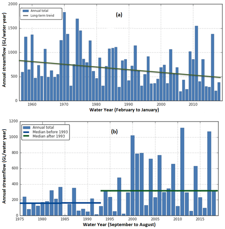
Figure 5 Typical examples of (a) trend and (b) step change in annual streamflow in southern and northern Australia.

Medians of slopes for annual and seasonal streamflow were located close to or above zero for drainage divisions in the northern part of Australia (Fig. 4b). The highest (+7.13 mm yr⁻¹ yr⁻¹) trend line slope occurred in the summer (December–February). The median of trend line slopes in summer (+1.02 mm yr⁻¹ yr⁻¹) is higher than that in the other three seasons (all <0.01 mm yr⁻¹ yr⁻¹) in the northern divisions. Streamflow in all seasons, except in summer, showed negligible trends in the northern parts of Australia. More than 90 % of the annual streamflow volumes in the northern drainage divisions occur in summer and autumn (December–May). For annual flows, slopes were between +12.1 and −6.0 mm yr⁻¹ yr⁻¹ (Fig. 4b), and the median of slopes was approximately +1.46 mm yr⁻¹ yr⁻¹. Figure 5a shows a typical example of linear trend analysis using the Theil–Sen approach for annual streamflow in southern Australia.

4.1.2 Monotonic trend – short-term persistence (STP) and long-term persistence (LTP)

Streamflow data from stations that are significantly autocorrelated (lag 1 or more) at p<0.10 and H values that are significant at p<0.10 are considered to have short-term persistence (STP) and long-term persistence (LTP) respectively. To analyse the presence of STP and LTP, results from the MK3 and MK4 tests were examined respectively. In the South East Coast (II), South West Coast (VI) and southern Murray–Darling Basin (IV) divisions, most stations showed significant STP, LTP, or both STP and LTP for the water year and for all four seasons (Fig. 6). Across water years and all seasons, the percentage of stations with STP was greater than that with only LTP or that with both STP and LTP. For water years, data from 88 % of stations showed STP and data from 28 % of stations showed LTP across Australia. However, LTP was evident mainly in the southern and south-eastern parts of Australia (divisions II, III, IV, V, VI) and in the north in the Carpentaria Coast (IX) division. Seasonally, autumn had the highest number of stations (221) with LTP persistence.

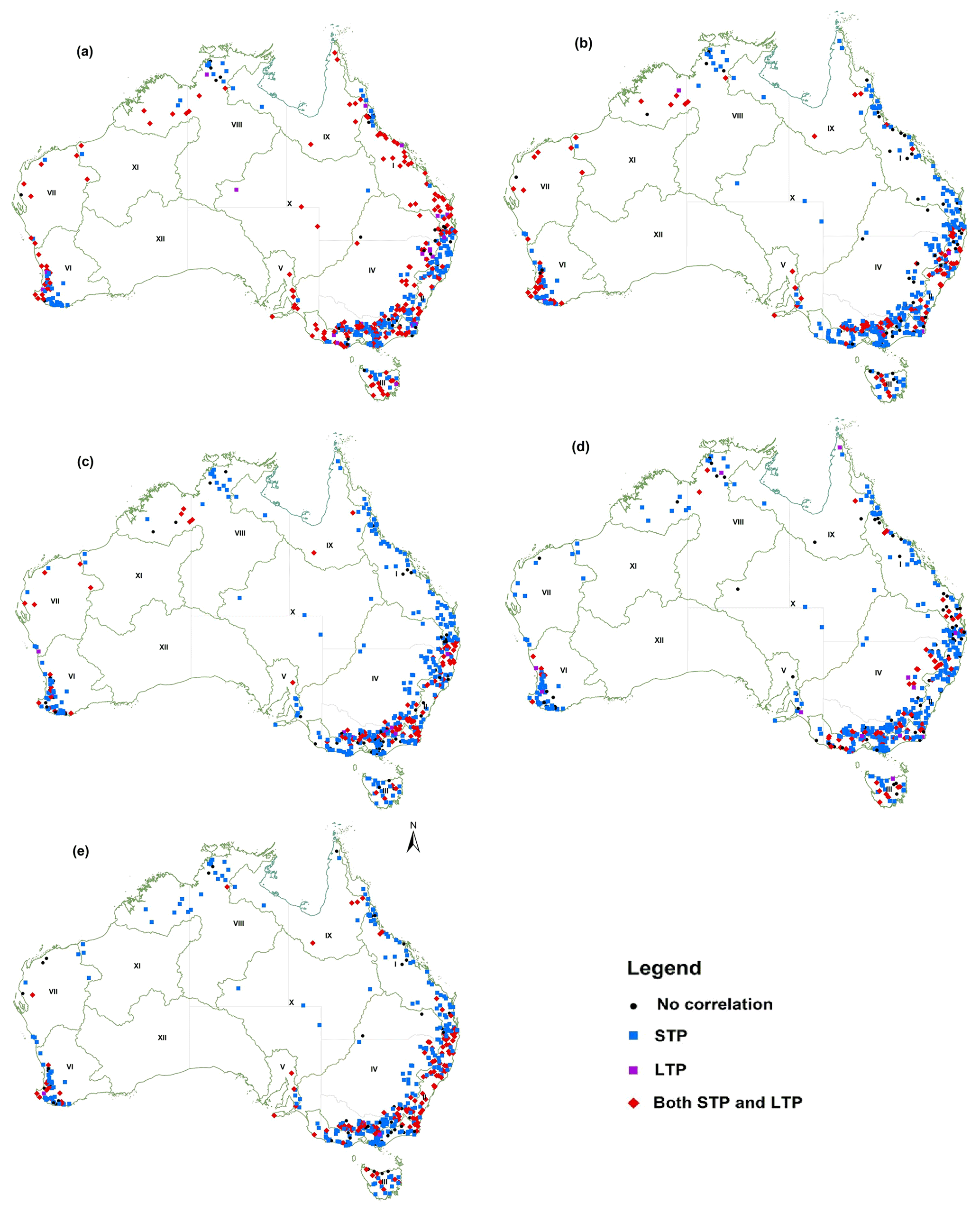
Figure 6 Spatial distribution of stations where streamflow shows persistence, short-term persistence (STP) and long-term persistence (LTP), in (a) autumn (March–May), (b) winter (June–August), (c) spring (September–November), (d) summer (December–February) and (e) annually (water year) at p<0.10.

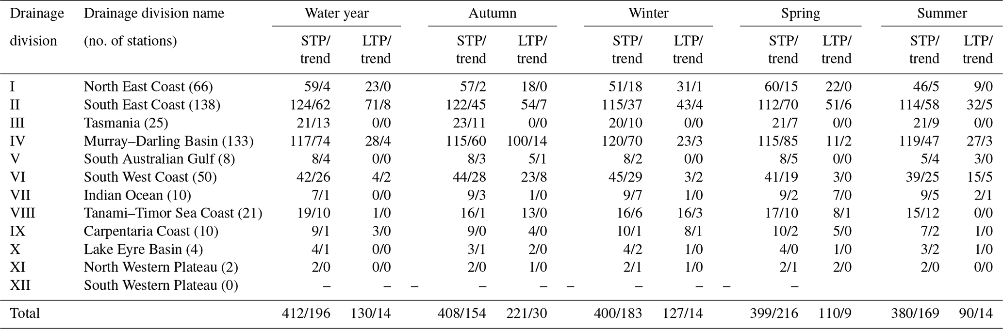
Data from stations with a significant correlation at p<0.10 with STP and LTP were tested for trends (Table 3) using the MK3 and MK4 tests respectively. Of the 412 stations with significant STP across water years, 196 stations showed trends from the MK3 test. Of the 130 stations with data showing significant LTP, 14 had significant trends from the MK4 test. In drainage divisions II to VI in the south, nearly half of the stations showed significant trends with STP. However, results vary slightly across different drainage divisions for the four seasons. In autumn, 33 % of the 87 % of stations with significant STP showed trends, whereas 6 % of the 47 % of stations with significant LTP showed trends. Similarly, in winter, 39 % of the 86 % of stations with significant STP showed trends, whereas 3 % of the 27 % of stations with significant LTP showed trends. In spring, 44 % of the 85 % of stations with significant STP showed trends, whereas 2 % of the 24 % of stations with significant LTP showed trends. In summer, 36 % of the 81 % of stations with significant STP showed trends, whereas 3 % of the 19 % of stations with significant LTP showed trends.

Table 3 Summary of stations with short-term persistence (STP) and long-term persistence (LTP) of streamflow and of stations that showed trends using the MK3 and MK4 tests across drainage divisions for the water year and the four seasons at p≤0.10. The numbers in each column show the STP or LTP and the trend (as stated in each respective column) separated by a slash.

4.1.3 Monotonic trends – MK tests

Table 4 summarizes the MK3, MK3bs and MK4 test results. Figure 7 shows the distribution of trends for each drainage division for the water year, autumn, winter, spring and summer for all three MK tests. The MK3 test results are similar to the MK3bs test results for water years and all four seasons, as they both consider the full autocorrelation structure (STP) of the streamflow series. The spatial distribution of trends using all three MK tests in the water year suggests that the annual mean streamflow has increased in the Tanami–Timor Sea Coast division in northern Australia, whereas it has decreased in the south-western and south-eastern parts of the country (Fig. 7). The magnitude trends in streamflow volumes expressed by the Theil–Sen slope show a maximum increase of 2.4 % yr⁻¹ at one station in the Tanami–Timor Sea Coast (VIII) division and a maximum decrease of −3.9 % yr⁻¹ at one station in the Murray–Darling Basin (IV) division over a period of at least 50 years. The MK3 test results are almost like those of the MK3bs test for water years and all four seasons, as they both consider the full autocorrelation structure (STP) of the streamflow series. Therefore, the MK3 test results are initially analysed.

Table 4 Results of the three Mann–Kendall (MK) tests, MK3, MK3bs and MK4, for the water year and all four seasons. The numbers in each column represent the number of stations with increasing trends (denoted using “+”) and the number of stations with decreasing trends (denoted using “−”) separated by a slash.

Entries in bold indicate results that are regionally significant at p<0.10.

Figure 7 Maps showing seasonal trends using the (a) MK3, (b) MK3bs and (c) MK4 tests. Results are reported for autumn, winter, spring, summer and annually (water year) (p<0.1). Upward-pointing triangles (green) indicate significant increasing trends, and downward-pointing triangles (red) indicate significant decreasing trends. Grey dots indicate stations with no trends. Drainage divisions with positive and negative trends with regional significance at p<0.10 are coloured blue and yellow respectively.

Although most of the 467 streamflow stations showed trends, only 14 stations had data with increasing trends across water years, and 212 stations showed decreasing trends that were statistically significant (Table 4). With respect to water year, more than 50 % of stations with increasing trends were located in the Tanami–Timor Sea Coast (VIII) drainage division. Streamflows that showed decreasing trends were within the South East Coast (II), Tasmania (III), Murray–Darling Basin (IV), South Australian Gulf (V) and South West Coast (IV) drainage divisions. Most stations in other divisions showed no significant trend (Fig. 7)

For autumn (March–May), streamflows at more than 50 % of stations showed significant trends in the South East Coast (II), Tasmania (III), Murray–Darling Basin (IV), South Australian Gulf (V), South West Coast (IV) and North East Coast (I) divisions. Other divisions showed autumn decreasing trends that were very similar to those found across water years, except for the Tanami–Timor Sea Coast (VIII) in the north, where only one station showed an increasing trend. Data from 173 stations showed significant trends across water years, 4 of which were increasing and 169  of which were decreasing (Table 4). In autumn, the maximum increase in streamflow was 1.3 % yr⁻¹, and the maximum decrease was −5.8 % yr⁻¹. Both trends were at stations in the South West Coast (IV) division.

Across winter (June–August), streamflows at over half of the stations showed significant decreasing streamflow trends in the North East Coast (I), Tasmania (III), Murray–Darling Basin (IV), and South West Coast (IV) divisions, whereas they showed significant increasing trends in the Tanami–Timor Sea Coast (VIII) division. However, in the South East Coast (II), Pilbara–Gascoyne (VII), Carpentaria Coast (IX) and the Lake Eyre Basin (X) divisions, fewer than 50 % of stations had flows with significant trends. A total of 189 stations showed significant streamflow trends (for MK3) across Australia, 9 of which were increasing trends and 180 of which were decreasing trends (Table 4). The maximum increase in winter flows was 2.3 % yr⁻¹ (in the Tanami–Timor Sea Coast (VIII) division) and the maximum decrease was −3.4 % yr⁻¹ (in the Murray–Darling Basin (IV) division). For stations in the Murray–Darling Basin (IV) division, significant trends varied between −0.5 % and −3.4 % (median of −1.3 % yr⁻¹).

Spring (September–November) saw more stations with decreasing flow trends compared with water years or the other seasons. Trends in flow were mostly detected at stations in all divisions except for Lake Eyre Basin (X) and North Western Plateau (XI), for which there is very limited flow data. The South East Coast (II) and Murray–Darling Basin (IV) divisions had the highest number of stations with decreasing trends in streamflow, compared with trends in the water year and other seasons (Table 4). There were stations in the South East Coast (II), Tasmania (III), Murray–Darling Basin (IV) and South Australian Gulf (V) that showed significant decreasing trends. For spring (September–November), 235 stations showed significant trends: 8 increasing and 227 decreasing (Table 4). The maximum increase in spring flows was 3.1 % yr⁻¹ (in the Tanami–Timor Sea Coast (VIII) division), and the maximum decrease was −2.8 % yr⁻¹ (in the South West Coast (IV) division).

For summer (December–February), stations in the Tanami–Timor Sea Coast (VIII) division showed significant increasing flow trends, as with trends in other seasons. Stations in the South East Coast (II), Tasmania (III), Murray–Darling Basin (IV), South Australian Gulf (V) and South West Coast (VI) divisions showed significant decreasing trends in flow. In summer, 175 stations showed significant flow trends: 26 increasing and 149 decreasing (Table 4). The maximum increase in summer flows was −2.1 % yr⁻¹ (in the Tanami–Timor Sea Coast (VIII) division) and the maximum decrease was −5.0 % yr⁻¹ (in the South West Coast (IV) division).

While results from the MK3 and MK3bs tests are nearly identical for most cases, MK3 and MK4 do show differences for most annual and seasonal flow statistics. A typical example of the MK3bs statistic obtained from 2000 samples from two locations with (a) decreasing and (b) increasing trends is shown in Fig. 8. It illustrates how the observed values are located below or above the 5th and 95th percentiles respectively. A small number of stations have significant streamflow trends when LTP behaviour (MK4) is considered (Fig. 7, Table 4). This is particularly evident in the South East Coast (II) division for water years and in the Murray–Darling Basin (IV) division for autumn (Fig. 7, Table 4). The MK4 test resulted in more stations with trends in winter and spring, compared with autumn and summer. Across Australia for water years, 14 stations showed significantly increasing trends in flow, and 196 stations showed significantly decreasing trends, slightly less than the MK3 and MK3bs test results (Table 4). Similar results are also evident for the four seasons across Australia (Table 4).

Figure 8 Examples of histograms for two stations representing the frequency distribution of the MK statistic (S) obtained from 2000 samples of moving block bootstrap iterations; red triangles are observed values, and dotted lines show the 5th and 95th percentiles for (a) a decreasing trend and (b) an increasing trend in the Tasmania (III) and Carpentaria Coast (IX) divisions respectively.

4.2 Step change

The nonparametric Pettitt test (Pettitt, 1979) was used to test for step changes for water years as well as for all seasons. This test is biased towards finding step changes in the centre of a time series (Mallakpour and Villarini, 2016). As the annual streamflow has a skewed distribution and possibly has outliers, this nonparametric test, which is least sensitive to these characteristics, is well suited to change-point detection. A typical example of step change in northern Australia is shown in Fig. 5b. Step-change maps (Fig. 9a) clearly reveal a spatial pattern in the location of stations that exhibited a significant step change in flow. The direction and significance of step changes are consistent with results from the MK tests (Fig. 7) for most stations. Years when step changes occurred show spatial groupings within several drainage divisions. Significant step changes or shifts across water years as well as for all four seasons for each drainage division are summarized in Table 5. For water years, the South East Coast (II), Murray–Darling Basin (IV), South Australian Gulf (V), South West Coast (VI) and Tanami–Timor Sea Coast (VIII) drainage divisions all showed significant step changes for more than 60 % of station flows (Fig. 9a, Table 5). Increasing shifts were seen in northern Australia, including the Indian Ocean (VII), Tanami–Timor Sea Coast (VIII) and Carpentaria Coast (IX) divisions, whereas decreasing shifts were seen in all drainage divisions except for the Tanami–Timor Sea Coast (VIII), Carpentaria Coast (IX) and North Western Plateau (XI). The South East Coast (II), Murray–Darling Basin (IV), South West Coast (VI) and Tanami–Timor Sea Coast (VIII) divisions had significant step changes across water years (Fig. 9).

Table 5 Annual and seasonal shifts in different drainage divisions using a Pettitt test at p<0.10. The numbers in each column represent the number of stations with increasing shifts (denoted using “+”) and the number of stations with decreasing shifts (denoted using “−”) separated by a slash.

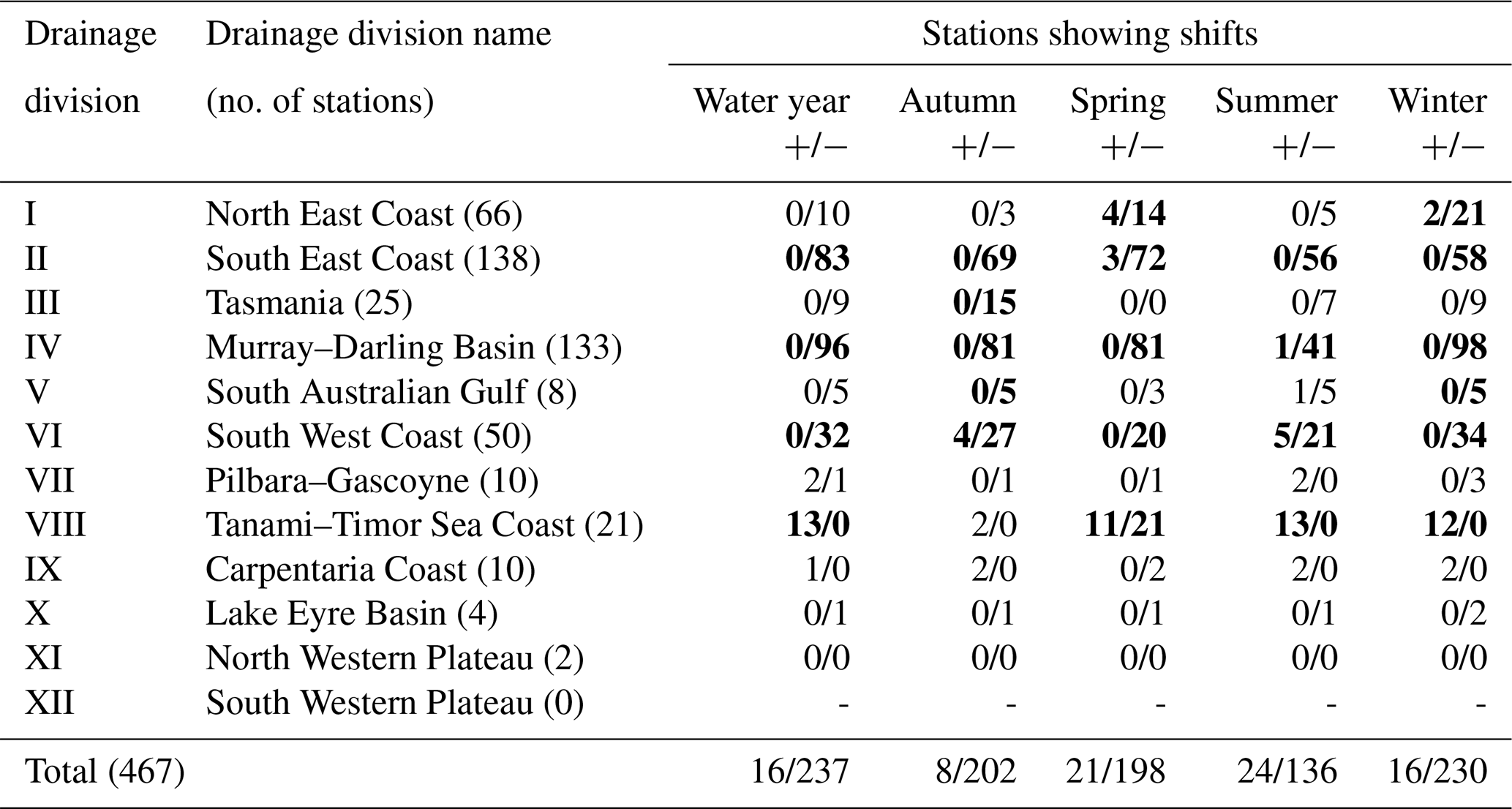
Entries in bold indicate results that are regionally significant at p<0.10.

Figure 9 (a) Map showing stations with step changes in flow across each season and water year (at a significance level of p<0.1). Upward-pointing green triangles and downward-pointing red triangles represent upward and downward step changes respectively, whereas black dots refer to sites without significant shifts. Drainage divisions with positive and negative shifts with regional significance at p<0.1 are coloured blue and yellow respectively. (b) The number of stations with significant step changes in flows (p<0.1) across each season and water year.

For summer (December–February), the lowest proportion of stations had significant step changes in flow compared with the other seasons or with water years (Table 5). The South East Coast (II), Murray–Darling Basin (IV) and South West Coast (VI) divisions had significant step changes at p<0.10 for water years and for all seasons, while the Tanami–Timor Sea Coast (VIII) division had step changes for water years and all seasons except for autumn. Tasmania (III) had significant step changes only in autumn. The North East Coast (I) division had significant step changes in spring and winter. The South Australian Gulf (V) division had significant step changes in autumn and winter (Fig. 9).

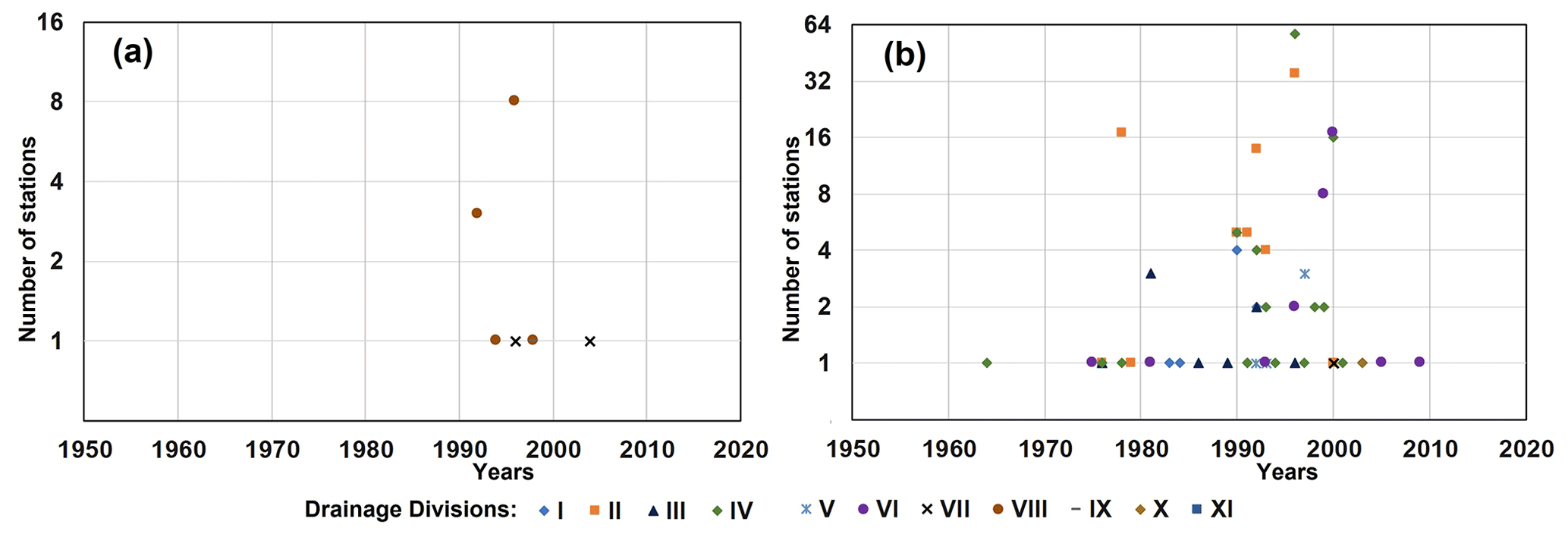
Figure 10 The timing of step changes and the number of stations with step changes for different drainage divisions with (a) increasing and (b) decreasing changes in the water year.

Figure 9 shows the number of stations with step changes in flow, each year between 1950 and 2018, for water years and for each season. The first step change was detected in 1964, and most changes occurred between 1970 and 1999. Of 467 stations, a total of 253 stations showed step changes in flows for water years (p<0.10), 16 of which were increasing and 237 of which were decreasing changes in flows. Water years between 1992 and 2004 showed increasing step changes at 16 stations, with the water-year 1996 having 9 stations with increasing step changes in flow (Fig. 9b). The period from 1975 to 1979 showed decreasing step changes for 24 stations, 18 of which were in the 1978 water year. The period from 1981 to 1989 showed decreasing step changes for 8 stations, and the period from 1990 to 2000 showed decreasing step changes at 190 stations, half of which occurred in the 1996 water year.

Autumn (March–June) had a total of 210 stations with step changes (p<0.10) in flow, 8 of which were increasing and 202 of which were decreasing. The first increasing step change in autumn was detected in 1970 (Fig. 9b), in the Carpentaria Coast (IX) division. Similar to water years, most step changes occurred between 1990 and 2000, with 147 stations showing decreasing step changes in flow (Table 5). About one-quarter of the step changes took place in the 1996 water year.

In winter (June–August) 246 stations showed a step change (p<0.10) in flow, 16 of which were increasing and 230 of which were decreasing. The first step change in winter occurred in 1970 (Fig. 9b). One station showed increasing shifts starting early in the 1970s, and 10 additional stations showed increasing shifts starting between 1996 and 1999. During the period from 1975 to 1982, 10 stations showed decreasing step changes in flows. Between 1990 and 2000, 211 stations (the largest in total) showed decreasing step changes in flows, with 101 of these changes occurring in 1996.

Spring (September–November) had a total of 219 stations with step changes (p<0.10) in flow, 21 of which had an increasing step change and 198 of which had a decreasing shift. The period from 1994 to 1997 saw 11 stations with increasing step changes (Fig. 9b), and 178 stations had decreasing step changes in their spring flows in the period from 1989 to 2001.

Summer had a smaller number of stations (160 out of 467) with step changes (p<0.10) in flows, 24 of which had increasing shifts and 136 of which had decreasing step changes (Fig. 9b, Table 5). The distribution of stations with step changes varied across the period of record: 28 stations had decreasing step changes during 1976–1989, 4 stations had increasing step changes during 1980–1988, 101 stations had decreasing step changes during 1992–2002 and 18 station had increasing step changes during 1990–2000 (Fig. 9b).

Figure 10 shows the timing of step changes for several drainage divisions where the water years mostly range from 1976 to 2009. The period from 1990 to 2000 showed decreasing step changes for 199 stations, mostly in the South East Coast (II), Murray–Darling Basin (IV) and South West Coast (VI) divisions. Most increasing step changes are in the Tanami–Timor Sea Coast (VIII) division during 1992–1998. The South East Coast (II), Murray–Darling Basin (IV), South West Coast (VI) and Tanami–Timor Sea Coast (VIII) divisions showed a greater number of stations with step changes distributed across the study period, indicating a higher association with natural changes and climate variability than for other regions (Table 5).

After the step changes, the distribution of mean monthly streamflow within a water year changed across all drainage divisions. The distribution of mean monthly streamflow at four selected gauging stations from four drainage divisions is shown in Fig. 11. In the northern part of Australia, the increase in streamflow is well distributed over most of the months. However, in south-western Queensland and the southern part of Australia, there seems to be a phase shift as well.

Figure 11 Distribution of mean monthly streamflow before and after step changes at four selected gauging stations representative of the (a) Tanami–Timor Sea Coast (VIII), (b) North East Coast (I), (c) Tasmania (III) and (d) South West Coast (VI) divisions; see Fig. 1 for locations.

4.3 Trend summary of regional significance – drainage divisions

Table 6 summarizes the regional significance of monotonic trends and step changes within each drainage division (at the drainage division scale) for water year and each of the four seasons. The Murray–Darling Basin (IV), South East Coast (I) and South West Coast (VI) divisions experienced decreasing trends for water year as well as for all seasons across all statistical tests. Similarly decreasing trends were also evident in the North East Coast (I), Tasmania (III) and South Australian Gulf (V) divisions with the exception of only a few statistical tests (Figs. 7, 9). In the North East Coast (I) division, only the MK3 test detected no significant annual trends. In the Tasmania (III) division, no step changes (PT) nor monotonic trends (MK4) were detected for spring and summer respectively. In northern Australia, the Tanami–Timor Sea Coast is the only division where most of the statistical tests show increasing trends for water years and for all seasons (Table 6). At annual scales, the MK3bs, MK4 and PT tests showed a significant increasing trend. With the exception of autumn, the MK3 and PT tests detected increasing monotonic trends for the other three seasons. There were no noticeable patterns in divisions in central Australia, including the North Western Plateau (XI) and Lake Eyre Basin (X) divisions. Trends in the Carpentaria Coast (IX) division were varied, and only summer saw a significant decreasing trend in flows (MK3). The lack of streamflow observations and relatively low number of stations, the length of records, or the number of non-zero-flow days in these central Australian divisions may play a role in detecting the trend.

Table 6 Summary of regional significance across different drainage divisions for water year and the four respective seasons.

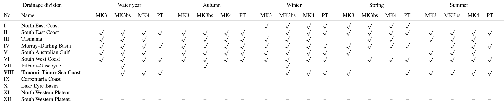
MK3, MK3bs and MK4 correspond to MK tests. PT corresponds to a Pettitt test. Entries in bold and roman font indicate respective positive upward and negative downward trends at p<0.10.

5 Discussion

5.1 Data quality and gap filling

To maintain the quality of streamflow data, only gauging stations with less than 25 % of flow volume above the recorded maximum gauged discharge and less than 10 % of infilled flow volume were included in this study and in the Hydrologic Reference Stations service. A quantitative evaluation of the accuracy of the gap-filling procedure showed that gap filling by interpolation or simple rainfall–runoff modelling is most accurate and effective if the missing record is less than 10 % (Zhang and Post, 2018), which was followed in this study. However, when the percentage of gap-filled data represent the relatively high end of the flow volume, the uncertainty becomes higher. McMahon and Peel (2019) analysed uncertainties associated with streamflow by considering the gauged and extended range of the stage–discharge relationship from 622 rating curves for 171 of the HRS gauging stations. They found that estimated flow volumes beyond the gauged range of the rating curve occurred at many of these gauging stations and caused measurement uncertainty. As our analysis is limited to seasonal and annual totals, implications of the estimated volumes beyond the gauged range may be minimal.

5.2 Comparison of different tests

The MK3 and MK4 tests show that there are strong autocorrelations or short-term persistence (STP) and significant long-term persistence (LTP) respectively in Australian streamflow in most drainage divisions (Fig. 6, Table 3). About 85 % of stations had data with a significant autocorrelation structure (Table 3), and about 40 % of these stations had more than lag-1 autocorrelation (Fig. 3). As such, the MK2 test (Kumar et al., 2009; Su et al., 2018) was not considered in the analysis, as it considers only the lag-1 autocorrelation structure. Around 30 % of stations had significant LTP only (Table 3). Therefore, two variations of MK3, which considers the total autocorrelation structure (STP), and MK4, which considers LTP behaviour, were used in the analysis. Our calculated trends are strongly affected by STP and LTP factors. For water years, there was a clear reduction in the number of stations with significant streamflow trends when the full autocorrelation structure (MK3) and LTP behaviour (MK4) were considered in the analysis: 263 stations with MK1, 226 with MK3 and 210 with MK4. A similar reduction was observed for most of the seasons (Table 4). Around half of stations with STP and only about 12 % of stations with LTP had significant trends for water year as well for all four seasons. The application of these different MK tests helped to differentiate trends that exist under the assumption of serial independence and short- and long-term persistence.

The Pettitt test showed that 54 % of stations experienced an abrupt shift in streamflows across water year. Most of these step changes (51 %) were decreases and were observed at more stations than for monotonic decreasing trends (38 %). Most of the increasing step changes took place in spring (September–November) and summer (December–February), whereas most of the decreasing step changes occurred in winter (June–August). The period from 1970 to 1999 had the largest number of step changes for water-year flows. The greatest number of stations (21 %) with a decreasing step change was found in 1996, whereas most of the increasing shifts (2 %) occurred in 1996. Seasonally, a greater number of stations with significant decreasing step changes in flow occurred in winter (Figs. 9b, 10).

5.3 Attribution of trends

For annual timescales, monotonic trends and step changes were similar in direction across the country; however, slight variation in direction was observed between seasons and different river basins. These results are consistent with previous findings from other studies on Australian streamflows (Zhang et al., 2016), despite having a larger number of gauge locations in all drainage divisions except the South West Plateau, different analyses methods, and different lengths and coverage periods of data (Durrant and Byleveld, 2009; Petrone et al., 2010; Tran and Ng, 2009). These findings are also consistent with the following observed changes in rainfall in different parts of Australia (BoM and CSIRO, 2020): (i) northern Australia has become wetter, particularly in the north-west, with rainfall generally above average in the dry seasons; (ii) Australia's climate has warmed on average by about 1.5 ^∘C since national records began in 1910, leading to an increase in the frequency of extreme heat events and in the length of the fire season across large parts of the country since the 1950s, especially in southern Australia; (iii) for April to October rainfall, there has been a decline of around 16 % in the south-west of Australia since 1970 and a decline of around 12 % in the south-east of Australia since the late 1990s; (iv) rainfall and streamflow have increased across parts of northern Australia since the 1970s (State of the Climate, 2020). In general, observed patterns of rainfall change across the country are expected to continue (BoM and CSIRO, 2020). Research has revealed the association of historical rainfall and soil moisture changes with observed streamflow across different drainage divisions of Australia (Wasko et al., 2021; Wasko and Nathan, 2019). Data from this national network of hydrologic reference stations will be useful for examining and detecting these associations.

Monotonic changes in streamflow may generally occur in response to long-term changes in the flow generation processes, including increases or decreases in rainfall, evapotranspiration, temperature, humidity and changes in vegetation dynamics. Note that the catchments considered here are unimpaired, so the impacts of anthropogenic activities are not significant. For some of the locations, the decreasing step changes coincide with the Millennium Drought between 1997 and 2009, but some catchments underwent changes a few years before that period (Fig. 10). Streamflow deficits in the Murray–Darling Basin were very large during the drought, with an estimated return period of 1 in 1500 years (Gergis et al., 2012), which may be one of the reasons for the largest proportion of stations (96 out of 133) depicting step changes. Sudden and abrupt changes, including step changes in the streamflow generation process, happen due to changes in thresholds, which are most prominent when the filling season begins, which is in autumn (March–June) in the south-west of Australia (Silberstein et al., 2012) including Tasmania (Fig. 9, Table 5). Also evident is a phase shift in the streamflow distribution in south-western Western Australia (Fig. 11d) due to a reduction in rainfall and lateral shift within the year (Silberstein et al., 2012). A reduction in winter rainfall, an increase in temperature and extreme rainfall are projected to continue in the future due to climate change (BoM and CSIRO, 2020). Climate change could make extreme events more frequent, causing an increasing streamflow trend for the wet season, a decreasing trend for the dry season and no trend for the annual basis. An increasing atmospheric CO₂ concentration may reduce evapotranspiration rates, which could lead to increased streamflow in certain climatic and geomorphic settings, and this may offset increased evaporation rates due to global warming (Krakauer and Fung, 2008). Recent studies covering south-eastern Western Australia have suggested that the increase in evapotranspiration per unit of rainfall plays an important role in streamflow reduction (Fowler et al., 2022; Peterson et al., 2021). However, questions still remain regarding how these changes in driving climate forces will interact with each other, and with vegetation, to guide the types and rates of change in the streamflow trend.

5.4 Management and further research

The frequency and magnitude of extreme rainfall events have increased across Australia (Sharma et al., 2018), and further investigation is required to understand how this translates to maximum flow and flood extremes in different parts of the country. Changes in the frequency and duration of low flows are also of interest to water managers, particularly in maintaining environmental water flow requirements. Questions remain in relation to phase shifts in streamflow generation within the year (Fig. 11), in particular in the southern part of Australia. For example, are these shifts related to rainfall distribution alone or are there other contributing factors, such as changes in temperature or secondary changes in vegetation dynamics? The influence of step changes on gradual trends was not considered in this study. Further investigation to identify the conditions and processes that result in these step changes would be of great value. Research into these questions is important to guide better management of water resources, infrastructure development and environmental water allocation. The statistical analysis undertaken in this study depends on the length of the time series available, which varies from one station to the next (Fig. 1). In future analyses, streamflow data obtained before the 1950s should be considered in order to identify decadal persistence, variability and trends. A better understanding of the nature of trends and step changes in seasonal streamflow can support better regional water management to regulate the flows and maintain adequate levels in reservoirs during dry and wet periods.

6 Summary and conclusions

Trends in annual and seasonal streamflow over Australia at 467 high-quality gauging stations listed in the Bureau of Meteorology's Hydrologic Reference Stations service were analysed and presented. The length of the daily streamflow data record ranged from a minimum of 30 years to a maximum of 69 years. Monotonic trend analyses were performed using three different forms of the Mann–Kendall test: a variance correction approach (MK3), a block bootstrap approach (MK3bs) and a long-term persistence approach (MK4). Identification and detection of step changes for seasonal and annual streamflow were accomplished using a nonparametric Pettitt test. The regional significance of these changes was analysed at the drainage division scale for different divisions and synthesized using a Walker test.

Monotonic decreasing trends in annual and seasonal streamflow at most of the gauging stations were detected in the Murray–Darling River basin and other drainage divisions in New South Wales, Victoria and Tasmania. Similar results were observed in south-western Western Australia, South Australia and in north-eastern Queensland. Decreasing trends in annual totals and in totals for all four seasons were also regionally significant at the drainage division scale. Only the Tanami–Timor Sea Coast drainage division in northern Australia showed increasing trends and step changes in annual and seasonal streamflow, and these were regionally significant. There were no significant spatial nor temporal patterns observed in central and mid-west Western Australia. One possible reason for this is the sparse density of streamflow stations and the length of the data record available for analysis.

In general, step changes were similar to the direction of monotonic trends across Australia. Only a handful of stations in northern Australia showed significant step-change increases in streamflow. At regional scales, that increasing trend was only statistically significant in the Tanami–Timor Sea Coast drainage division. Across southern Australia, most step changes occurred during the period from 1970 to the 1990s, with the majority of them being in 1990s, before the onset of the Millennium Drought in 1997. Most of the step changes occurred just at the start of winter when the rainy season begins.

Further investigation and research would assist in understanding the processes that govern the detected changes in flow generation, catchment memory and its interaction with rainfall change, increase in temperature and vegetation growth, and evapotranspiration.