the Creative Commons Attribution 4.0 License.
the Creative Commons Attribution 4.0 License.
 | 03 May 2023
Water and energy budgets over hydrological basins on short and long timescales
Samantha Petch
Tristan Quaife
Robert P. King
Keith Haines
Quantifying regional water and energy fluxes much more accurately from observations is essential for assessing the capability of climate and Earth system models and their ability to simulate future change. This study uses satellite observations to produce monthly flux estimates for each component of the terrestrial water and energy budget over selected large river basins from 2002 to 2013. Prior to optimisation, the water budget residuals vary between 1.5 % and 35 % precipitation by basin, and the magnitude of the imbalance between the net radiation and the corresponding turbulent heat fluxes ranges between 1 and 12 W m−2 in the long-term average. In order to further assess these imbalances, a flux-inferred surface storage (Sfi) is used for both water and energy, based on integrating the flux observations. This exposes mismatches in seasonal water storage in addition to important inter-annual variability between GRACE (Gravity Recovery and Climate Experiment) and the storage suggested by the other flux observations.
Our optimisation ensures that the flux estimates are consistent with the total water storage changes from GRACE on short (monthly) and longer timescales, while also balancing a coupled long-term energy budget by using a sequential approach. All the flux adjustments made during the optimisation are small and within uncertainty estimates, using a χ2 test, and inter-annual variability from observations is retained. The optimisation also reduces formal uncertainties for individual flux components. When compared with results from the previous literature in basins such as the Mississippi, Congo, and Huang He rivers, our results show better agreement with GRACE variability and trends in each case.
- Article
(13850 KB) - Full-text XML
- BibTeX
- EndNote


The terrestrial water cycle largely determines the Earth's climate and causes much of the natural climate variability. Variations in and long-term changes to the water cycle can have profound impacts on regional agriculture, ecosystems, and society. The surface energy budget is a key driver of the global water cycle, in addition to having a large influence over atmosphere and ocean dynamics and a variety of surface processes. Despite the fundamental importance to our understanding of climate and climate change, there remain some key challenges to quantifying the regional water and energy cycling rates. In particular, observations of the flux and storage terms tend to have large uncertainties and are inconsistent with budget considerations, while model estimates are internally consistent but usually show some mismatches to observations (e.g. Dong et al., 2020).
We assume the water balance by the following:
This states that the precipitation (P) falling over an area, combined with the loss of water to the atmosphere through evaporation (E) and the horizontal loss of water through runoff (Q), is balanced by the change in water storage in the area. The availability of GRACE (Gravity Recovery and Climate Experiment) satellite gravitational measurements of total water storage anomalies (S) since 2002 Tapley et al. (2019) has provided a valuable constraint to aid our understanding of the other water budget components. The previous literature has used the budget equation to test the accuracy of observations (Reeves Eyre and Zeng, 2021) and to validate model estimates (Long et al., 2015). Several studies also exist which use the budget equation to estimate one component while using observations for the other terms (Chen et al., 2020; Wang et al., 2015; Sheffield et al., 2009). For instance, Chen et al. (2020) provide a new estimate of seasonal and yearly river runoff changes for the Amazon basin by using the water budget closure method, and Rodell et al. (2011) use budget closure to estimate evaporation.
Recent developments in satellite retrievals have meant that budget closure can be assessed purely from remotely sensed data sources (Sheffield et al., 2009). However, water fluxes are still affected by considerable uncertainties, which have been highlighted in many water budget studies when independent products are combined. For example, Sheffield et al. (2009) used the budget equation, taking Q as a reference variable, and found significant errors that were larger than the observed Q taken from in situ measurements. A common approach among previous water budget assessments is to use a range of products for each flux component and evaluate the ability of different combinations to close the water budget. For example, Lehmann et al. (2022) investigated the budget closure at catchment scales using 11 precipitation, 14 evaporation, and 11 runoff datasets together with GRACE. The study concluded that no single combination of data sources can close the budget well for all regions. It was also highlighted that, in regions for which selected data sources did close the budget reasonably well, this could be as a result of the cancellation of errors. The multi-source strategy has the potential to compensate for the limitations of each individual estimation method in terms of its accuracy and spatiotemporal coverage. However, combining multiple sources can introduce a new challenge of how to allow for discrepancies between the different data products. Lehmann et al. (2022) determined uncertainties for each flux based on the inter-product spreads, which is the common way to treat uncertainties when multiple products have been used (e.g. Abolafia-Rosenzweig et al., 2021). Resolving the uncertainty among the various estimates for a specific variable remains an underlying challenge when using both in situ measurements and remote sensing observations (Pan et al., 2012).
Non-closure errors can come from the complexities of deriving energy and water fluxes from remote measurements. This process involves independent algorithms that use distinct observations and assumptions which can be subject to both random and systematic errors (L'Ecuyer et al., 2015). Since each flux dataset may be developed in isolation, valuable energy budget and water cycle closure information is lost. Then, reintroducing budget closure as a constraint may help to reduce biases in these datasets.
There are several studies in existence which produce best estimates for all components in order to close the budget (e.g. Sahoo et al., 2011). Different techniques are seen to impose closure constraints, such as Kalman filters (Pan et al., 2012; Zhang et al., 2018), post-filtering (Munier et al., 2014; Aires, 2014), and variational methods (Rodell et al., 2015; Hobeichi et al., 2020). Abolafia-Rosenzweig et al. (2021) focused on the human impacts on the water cycle and produced a remotely sensed ensemble of the terrestrial water budget (REESEN) containing 60 unique realisations of the water budget for basins between 50∘ N and 50∘ S, over October 2002–December 2014. Three different closure techniques were applied to all ensemble members in order to produce three ensembles of corrected budget estimates. Zhang et al. (2018) produced a climate data record (CDR) for the period 1984–2010, which provides monthly 0.5∘ resolution global estimates of each flux component, while closing the budget using a constrained Kalman filter.
Typically, these methods produce new monthly estimates for each flux by adjusting input observations according to defined errors either in order to achieve complete budget closure (Aires, 2014) or to achieve a budget residual within allowed errors (Hobeichi et al., 2020). Errors are often based on inter-product spread (Abolafia-Rosenzweig et al., 2021) or based on discrepancies with non-satellite data (Sahoo et al., 2011). Crude approximations are also sometimes used when representing errors; for example, Munier et al. (2014) supposed constant errors for P and E of 10 cm and 10 % of the mean discharge for Q. Such assumptions are made due to the absence of any comprehensive study that quantifies errors at the global or regional scales for each of the datasets used (Munier and Aires, 2018).
Zhang et al. (2018) adjust fluxes according to the deviation from the ensemble mean of all data sources for the same budget variable. In a post hoc adjustment, Zhang et al. (2018) also remove any long-term storage trend by redistributing the non zero mean between the precipitation and the evaporation in a way that maintains budget closure. However, most other studies that close the water budget on a monthly timescale fail to consider total water storage over longer timescales. The GRACE time series does provide water storage information on all timescales longer than 1 month, and so, when only using monthly changes as input, information can be lost. Post hoc detrending (Zhang et al., 2018) is also incorrect for regions where GRACE does detect a trend in storage; for example, Wang et al. (2015) found significant trends in water storage in 11 out of the 19 basins studied. In addition, GRACE data often reveal interesting inter-annual variations in basin water storage which will not necessarily be reproduced by most previous approaches (examples will be shown later). One key aim of this study will be to produce balanced water budgets which agree with the inter-annual variability and long-term trends observed by GRACE. Since the other fluxes of P, E, and Q are linked to via Eq. (1), the use of the additional information given by GRACE storage should also provide more accurate constraints on these fluxes. The problem considered here involves only linear budget equations, which means that there will always be a unique monthly solution that will not depend on the choice of the optimisation algorithm. The advance we present comes from the constraints imposed, and alternative optimisation algorithms should give the same results. To the authors' knowledge, no previous efforts have been made to fully fit flux estimates to GRACE during budget closure.
The surface energy balance can be described by the incoming energy from downwelling shortwave and longwave radiation (DSR and DLR, respectively), the outgoing energy from the longwave flux (ULW), and reflected shortwave flux (USW) and the turbulent heat fluxes latent and sensible heat (LE and SH, respectively). Fluxes are taken to be positive when directed towards the surface. Therefore, the energy budget can be written as follows:
where NET is the total energy absorbed by the surface.
The water and energy cycles are coupled due to the exchanges of latent heat that occur during precipitation and evaporation, and so we will also include a regional coupled energy budget closure in our analysis, with a particular focus on seasonal to inter-annual variability, and the interactions with the water cycle.
Without limitations on water availability, evaporation increases with increasing temperature which must be balanced by an increase in precipitation. Additionally, warmer air can hold more moisture, about 7 % more water vapour for each degree Celsius of warming, and so evaporation and precipitation are projected to intensify as a consequence of the changes in the Earth's energy balance (IPCC, 2013).
The coupling between the water and energy budgets enables them to provide constraints on one another; however, most previous studies have performed water or energy budget analyses independently. The NASA Energy and Water cycle Study (NEWS) derived an optimised coupled global–continental-scale budget, with Rodell et al. (2015) focusing on the water and parallel energy budget (L'Ecuyer et al., 2015), for the period 2000–2010, focusing on satellite-derived data as far as possible. Thomas et al. (2020) extended the NEWS coupled approach, focusing on improving ocean basin fluxes. Hobeichi et al. (2020) then developed a regional coupled approach over land areas, producing the Conserving Land–Atmosphere Synthesis Suite (CLASS), which solves for monthly water and energy budgets at 0.5∘ grid scale from 2003–2009.
Data-driven global flux estimates are subject to uncertainty due to the lack of energy balance closure. In order to mitigate this, some data sources look to account for energy balance within their products. For example, FLUXCOM products undergo three different energy balance closure corrections for LE and SH (Jung et al., 2019).
This study aimed to produce a new optimisation methodology which is able to account for both short and long timescales. Using this new methodology, this study produces optimised estimates for each of the water and energy budget components, based on observations. It aims to ensure that the estimates are consistent with GRACE on a monthly timescale, in addition to being in agreement with any inter-annual and long-term storage trends, and that the total energy lost or absorbed by the ground over this time period is small. The estimates are also constrained to close the monthly water budget, while accounting for the uncertainties in the observations. The paper is organised as follows: Sect. 2 describes the data used as input for the optimisation, Sect. 3 describes the methodology used in the study, and results are shown in Sect. 4. Optimisation uncertainties are included in Sect. 5, and a discussion is included in Sect. 6, before concluding in Sect. 7.
Each of the datasets described in this section has a monthly resolution and has been interpolated at a 0.5∘ spatial resolution and then masked and spatially averaged over different basins chosen in this study. Flux datasets represent the average flux over each calendar month and therefore are considered to represent the flux mid-month. The input data sources used are summarised in Table 1. For this study, data for each variable were downloaded for each month between October 2001 and December 2013.
Wielicki et al. (1996)Wiese et al. (2016)Jung et al. (2019)Adler et al. (2003)Ghiggi et al. (2019)
Other water budget studies have often used an ensemble of products to represent input observations in the absence of any widely accepted “best dataset”. In this study, we use only a single data product for each component, which we account for in our uncertainty calculations. We aimed to use Earth observation data where possible and sought global gridded products to ensure the uniformity of the uncertainties across all basins. Overall, the specific datasets chosen were not critical, as our primary goal was to evaluate our new optimisation methodology and its ability to bring independent products into consistency.
2.1 GRACE
Water storage data are taken from the Gravity Recovery and Climate Experiment (GRACE). GRACE measures changes in the Earth's gravity field, which is directly correlated to the change in surface mass and is indicative of water storage change. The water mass anomalies are expressed in terms of equivalent water thickness and represent the deviations of mass in terms of vertical extent of water in centimetres. All water storage compartments, including snow, surface water, soil moisture, and deep groundwater, are accounted for (GravIS, 2021).
The GRACE data were processed using an advanced mass concentration (mascon) approach that enables improved signal resolution relative to the standard spherical harmonic technique (Rodell et al., 2018). It acts across coarse spatial and temporal scales and requires filtering prior to being interpreted. The processing chain of GRACE data involves a large number of corrections and uncertainties that introduce errors and impose restrictions on its use (Swenson and Wahr, 2006). One of the most important errors is the signal leakage between neighbouring grid cells caused by the truncation of spherical harmonics and Gaussian filtering (Landerer and Swenson, 2012). The version used here is the Jet Propulsion Laboratory (JPL) Mascon RL06_v2, which uses a coastline-resolution improvement (CRI) filter applied to separate the land and ocean portions of mass within each land or ocean mascon in a post-processing step. The relative magnitude of ocean and land leakage errors is primarily a function of how the mascon placement conforms to the coastline. The CRI filter acts to reduces leakage errors across coastlines. Wiese et al. (2016) quantify the associated errors in determining mass variations for different basins. On average, measurement errors dominate leakage errors (mean error of 8.3 mm versus 5.1 mm), particularly for larger basins, as the fraction of fully contained mascons in the basins increases.
The data are provided with 0.5∘ resolution grids and time given as days since 1 January 2002 (00:00:00 Z). Storage values are provided per calendar month, but these must be converted into storage changes, dS, over each month. In the literature, several different methods have been used, such as centred difference schemes (Zhang et al., 2018), backwards difference schemes (Hobeichi et al., 2020), and fourth difference schemes (Reeves Eyre and Zeng, 2021). Here we use simple centred differences, , for month i.
There were a small number of months with missing data which were filled with monthly climatology plus the temporal interpolation of monthly storage anomalies.
2.2 GPCPv2.3
Precipitation data are taken from the Global Precipitation Climatology Project (GPCP) version 2.3 (see Adler et al., 2016a). GPCP provides monthly precipitation data from 1979–present and aims to provide a globally coherent dataset of precipitation (Adler et al., 2003). It combines observations and satellite precipitation data into 2.5∘ global grids. The product employs precipitation estimates from the 06:00 and 18:00 LT low-orbit satellite Special Sensor Microwave Imager (SSM/I) and Special Sensor Microwave Imager/Sounder (SSMIS) passive microwave data to perform a calibration of infrared data from the international collection of geostationary satellites in the latitude band 40∘ N–40∘ S. The satellites include the Geostationary Operational Environmental Satellites (GOES) from the National Oceanic and Atmospheric Administration (NOAA), and the calibration varies by month and location (Adler et al., 2016a). Absolute magnitudes are considered reliable, and inter-annual changes are robust. Precipitation may be underestimated in mountainous areas; however, version 2.3 has improved on this compared to previous versions (Adler et al., 2016a).
2.3 GRUNv1
Runoff data are taken from the Global Runoff Reconstruction (GRUN) dataset. GRUN provides a global gridded reconstruction of monthly runoff, covering the period 1902–2014 at a 0.5∘ spatial resolution (Ghiggi et al., 2019). The dataset uses a global collection of in situ streamflow observations to train a machine learning algorithm that predicts monthly runoff rates based on antecedent precipitation and temperature from an atmospheric reanalysis. The precipitation and temperature data are obtained from the Global Soil Wetness Project Phase 3 (GSWP3) dataset version 1.05 (Kim et al., 2017). The in situ runoff observations are derived from the Global Streamflow Indices and Metadata archive (GSIM; Do et al., 2018), which consists of 35 002 streamflow stations. Model validation is based on cross-validation experiments, using datasets such as the Global Runoff Data Centre (GDRC) reference dataset (GRDC, 2020) and runoff simulations from the Inter-Sectoral Impact Model Intercomparison Project (ISIMIP; Warszawski et al., 2014). Different metrics are used to assess the skill of the runoff reconstruction. For large GDRC river basins, the relative bias (which has an optimal value of 0) had a median of 0.047, the squared correlation coefficient, R2, had a median of 0.738, and the ratio of the standard deviations (optimal value of 1) had a median of 1.004. Overall, the agreement is said to be satisfactory, although there is a tendency to underestimate runoff rates when the magnitude increases (Ghiggi et al., 2019).
2.4 FLUXCOM
Latent and sensible heat data come from FLUXCOM, using the remote sensing plus meteorological/climate forcing (RS+METEO) setup. FLUXCOM uses machine learning to merge energy flux measurements from FLUXNET eddy covariance towers with remote sensing and meteorological data to estimate net radiation, latent and sensible heat, and their uncertainties. Using three different machine learning algorithms, energy balance closure correction constraints, and climate forcing data from various sources as predictors, a large ensemble of gridded flux products is generated (FluxCom, 2021). A lack of energy balance closure of around 20 % was observed across FLUXNET sites, which was addressed using three different approaches based on hypotheses regarding the primary cause of the energy balance closure gap. Closure corrections include the Bowen ratio correction, which assumes that the ratio of sensible and latent heat is accurately measured, and a residual approach, which reallocates missing energy to other flux components (Jung et al., 2019). The data are provided on 0.5∘ global grids. FLUXCOM ensemble products provide uncertainties per grid cell and time step. Uncertainties can arise from empirical upscaling, the choice of machine learning algorithm, and the predictor variables.
2.5 CERES
This study takes radiative flux data from the Clouds and Earth Radiative Energy System (CERES), a multi-satellite measurement programme for monitoring radiation. CERES instruments were designed to provide accurate measurements for the long-term monitoring of Earth's reflected shortwave and emitted longwave radiances, as part of its radiation energy budget (Loeb et al., 2016). Seven CERES instruments on five satellites have been launched (TRMM, Terra, Aqua, S-NPP, NOAA-20). Each CERES instrument has three channels, namely a shortwave channel to measure reflected sunlight, a longwave channel to measure Earth-emitted thermal radiation in the 8 to 12 µm window region, and a total channel to measure all wavelengths of radiation. Calibration sources on board include a solar diffuser, a tungsten lamp system with a stability monitor, and a pair of blackbodies that can be controlled at different temperatures (Wielicki et al., 1996). The CERES record is highly stable and has twice the spatial resolution and improved instrument calibration compared to the Earth Radiation Budget Experiment (ERBE) record (Acker et al., 2014). Here we use the latest version (CERES Energy Balanced and Filled (EBAF) Ed4.1). This version uses new clear-sky fluxes determined for the total region to determine top-of-atmosphere (TOA) and surface cloud radiative effects (CREs). Uncertainties are primarily determined by comparing EBAF surface fluxes with observations at surface sites over land and buoys over ocean (Kato et al., 2018).
2.6 Initial uncertainties
Many previous water budget studies have dealt with uncertainties by solving for multiple data products for each component and using the spreads as a measure of uncertainty. We have only used single data products here, although the uncertainties applied are based on prior studies that have taken multiple products to estimate uncertainties, in particular the NEWS analysis (L'Ecuyer et al., 2015; Rodell et al., 2015). Product uncertainties are very hard to estimate on regional scales because of unknown spatial error covariances. In situ, calibration-based errors may be correlated on small spatial scales but are likely to be uncorrelated on larger spatial scales. In addition, many product errors may scale with flux amplitudes, and some previous studies have therefore assigned uncertainties as a percentage of flux amplitudes.
Here, in order to give a traceable method, we have taken the continental-scale uncertainty estimates from the NEWS papers above and downscaled them to river basin scales, while assuming that errors are uncorrelated between river basin scales and continental scales. This leads to the following relationship between basin-scale and continental-scale flux uncertainties:
where σf is the basin-scale uncertainty for flux f over basin area a, and ΣF is the continental-scale uncertainty for flux F over continental area A. If the errors were assumed to correlate between scales, then the simpler uncertainty scaling as a percent of flux amplitudes would apply.
However, GRACE does not measure a flux but rather the strength of the gravitational field anomaly. To calculate the dS uncertainties, we use the basin values proposed by Wiese et al. (2016) for the JPL GRACE Mascon RL05M solution. Their method combines measurement uncertainty (ϵm) and leakage uncertainty (ϵl) to produce an uncertainty for storage (σS). We then calculate uncertainty in storage change between any 2 months (σdS), assuming errors are uncorrelated from 1 month to another, as follows:
We show examples of both input and optimised uncertainties later in the paper.
2.7 Study area and period
For this study, we focus on large river basins (see Fig. 1). The Mississippi, the Amazon, the Huang He (Yellow River), the Congo, and the Amur river basins are selected for more detailed analyses in this paper, based on storage trends seen in GRACE and overlapping regions with other studies to enable comparisons. Additional results for a larger range of basins are shown in the Appendix. This study is carried out for 2002–2013, due to the availability of the selected data products.
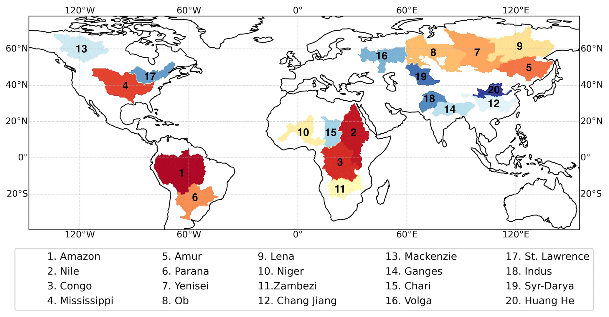
Figure 1Location of 20 selected large basins. Colouring is associated with basin size.
The basins selected capture a range of imbalances in their observed budgets from the initial data, including basins with strong inter-annual variability, basins from a variety of latitudes, and basins that have other optimised flux products already mentioned in the literature. We are also restricted to larger basins, preferably with simple basin boundaries, as these will have smaller GRACE storage errors, as described in Wiese et al. (2016).
3.1 Inferred storage from observations
For both water and energy budgets, we find it useful to calculate a surface storage anomaly, which we call the flux-inferred storage (Sfi), which is a time integral of the total fluxes in and out of a region. This quantity highlights flux imbalances, seasonal cycles, inter-annual variability, and trends very clearly and will also be used for developing the optimisations. For example, for water, we generate Sfi,w, using observations from the right-hand side of Eq. (1).
If we have an initial storage anomaly, then we can generate a storage by integrating with respect to time. For water, we take S[0] to be equal to the GRACE storage anomaly from 1 January 2002 and use this to initialise the Sfi,w time series.
If the initial fluxes were consistent with GRACE, then this should produce the GRACE time series, which prior to optimisation it does not. Also, if there are any persistent imbalances in the fluxes, then this shows up as a strong trend in Sfi,w. We also produce a detrended flux-inferred storage () in order to help emphasise imbalances in the seasonal storage cycle relative to GRACE.
A similar energy flux-inferred storage anomaly can also be generated from the energy balance (Eq. 2).
Again the Sfi,e will show up any seasonal cycle in surface warming, inter-annual variations, and long-term imbalances very clearly. A detrended flux-inferred energy storage (), which assumes the long-term NET to be zero, is also used in the optimisation to implement the long-term constraint.
3.2 Optimisation
Through an optimisation approach, we produce monthly estimates of the water and energy budget components aiming to satisfy the following: (1) minimise the distance from observed fluxes according to their relative uncertainties, (2) close the monthly water budget and long-term energy budget, (3) ensure the water and energy components are consistent, and (4) ensure the total water storage implied from our optimised fluxes has good agreement with the total water storage from GRACE. The reasoning behind step (4) and methods to achieve this are described in detail in Sect. 3.2.1.
When combining observations from independent data products described in Sect. 2, we see an imbalance in the monthly water budget (Eq. 1). For the energy budget (Eq. 2), we generally do not have a monthly estimate of NET against which to assess imbalances, although we do have an expectation that the long-term mean NET = 0; however, consider for the moment that monthly NET is also constrained. If we write the monthly water and energy budget variables in a column vector Fobs, where subscript “obs” denotes observed values, then Eqs. (1) and (2) can be expressed as a linear function of Fobs. Let A and B represent the water and energy budgets, respectively.
rw represents the water budget residual, and re represents the energy budget residual, which we will also write together as the residual vector R (appearing later). The optimisation acts to adjust the observed fluxes to close the budgets by redistributing rw and re to obtain R=0. We aim to find a new column vector F containing the optimised estimates we seek.
where a is a vector of the same size as F containing adjustments, such that and . In order to calculate F for month k, a cost function is set up as follows:
Closure constraints are imposed via the Lagrangian multipliers (λ and μ). Sobs is a covariance matrix containing flux variances on the diagonals. The off-diagonal elements would represent error covariance between input fluxes. In nearly all of the previous literature (Sheffield et al., 2009; Abolafia-Rosenzweig et al., 2021; Hobeichi et al., 2020), the covariance matrix is assumed to be diagonal (as shown in Eq. 11), although correlated errors may well be present due to the structural assumptions used for deriving Earth observation (EO)-based surface fluxes. We will discuss the potential impact of such error covariances in Sect. 6.
The cost function is minimised by setting the derivative with respect to each variable (F, λ, and μ) to zero. This results in the following constraints:
These constraints are then used to calculate values for μ and λ and solve for F via the least squares method.
The equations above allow us to balance water and energy budgets each month and can be solved independently every month, as has been done in the previous literature (Pan et al., 2012; Abolafia-Rosenzweig et al., 2021; Hobeichi et al., 2020). However, the resulting solutions will not necessarily give sensible longer timescale water or energy budgets. The optimised values of dS would not integrate to give a sensible trend or follow the observed variations in GRACE on longer timescales. Similarly, there is nothing to ensure that the integrated NET energy flux would remain realistically small, even if a monthly NET flux prior were available to use in the optimisation.
3.2.1 Sequential method for water budgets
One approach to imposing longer timescale constraints on the solution would be to make a single optimisation over all months together, simply by extending the F vector and including additional constraints on the sum of all the monthly water and energy storage changes. This may work well for energy where the only long-term constraint is on the NET energy flux, and this is the approach used by NEWS (L'Ecuyer et al., 2015); however, it would still not allow us to follow seasonal to inter-annual water storage information present in the GRACE data.
Instead, we opt for a sequential monthly approach. The monthly budget solutions are then not independent but take stock of previous optimisations in addition to the observed GRACE storage change from the start of the period up to the present time. The optimisation acts to minimise the distance of the Sfi,w generated from optimised fluxes with GRACE storage change at the end of each month, according to GRACE uncertainties. This constraint requires a term in the cost function of the following form:
which must be adapted in order to solve for . For an arbitrary month k, the optimised Sfi,w will be equal to the optimised Sfi,w for month k−1 plus the optimised for month k, as follows:
By using Eq. (16)to rewrite Sfi,w[k], we produce a term compatible with our cost function (Eq. 10) in order to impose the constraint described by Eq. (15), while solving for , as follows:
Note that implementing this constraint only requires adapting the Fobs vector in the cost function. This requires to be known when solving for month k, which is only possible when solving sequentially. The optimisation is performed for all months between January 2002 and October 2013. Figure 2 gives an overview of these steps.
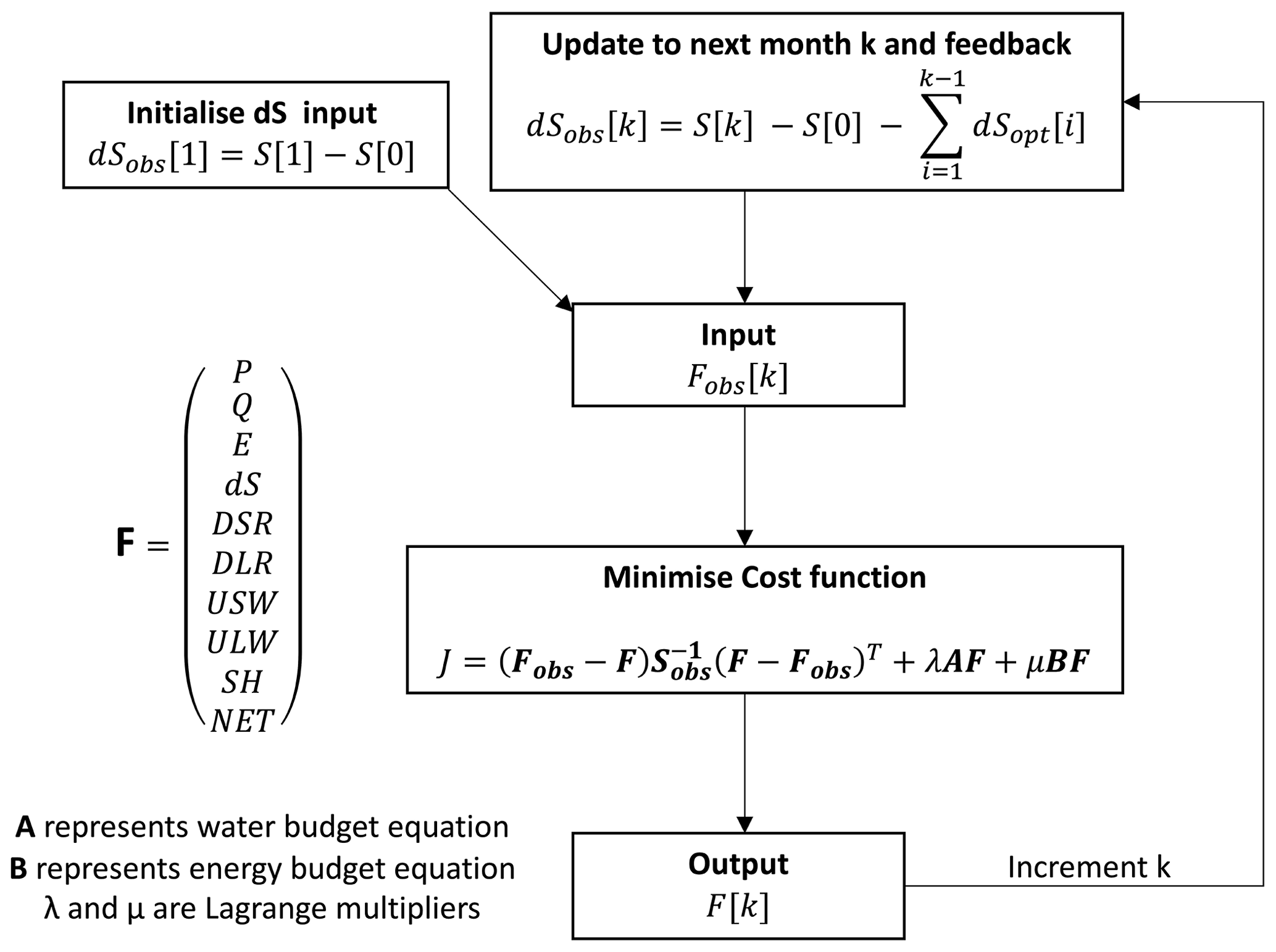
Figure 2Overview figure of the methodological steps.
The optimised fluxes are then integrated to produce the surface storage anomalies that they would imply, as described in Sect. 3.1, and are labelled as our “Optimised Storage” in the figures below.
3.2.2 Sequential method for energy budgets
Returning to Eq. (2), we note that, generally, we have no monthly constraints on either the surface energy storage or on the NET energy flux that could be used in a monthly optimisation. Although local measurements of ground heat flux are available from some flux tower sites which have been used in previous energy budget studies (Hobeichi et al., 2020), these NET fluxes are very poorly observed, associated with large uncertainties (even locally), and not available at basin scales. We have chosen not to use any independent NET prior and will comment on the consequent variability in the surface energy storage results.
We do apply a minimal constraint to the prior monthly energy fluxes, which aims only to give a small, long-term NET energy storage change during optimisation. To do this, we make use of the Sfi,e. When combining the observed energy fluxes to obtain NET and averaging over the whole time period, we see large imbalances, varying by basin (shown in Fig. 3). Therefore, when integrating NET over time to infer the Sfi,e, large trends are generally found (see Fig. 9).
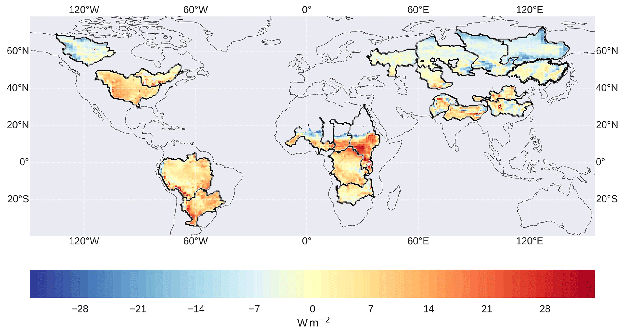
Figure 3NET downward energy flux derived from CERES radiative fluxes and latent and sensible heat fluxes from FLUXCOM, averaged over 2002–2013.
First, we detrend the Sfi,e, which is equivalent to removing the mean NET flux, to close the long-term energy budget, while preserving any inter-annual and seasonal variability. This detrended Sfi,e () is then used as a sequential monthly energy storage constraint in the same approach used to constrain the long-term water storage changes to GRACE in the previous section, using a cost function term during month k on NET[k], as follows:
This , based on the original fluxes, plays a similar role to the GRACE water storage change observations from the start to the current month and ensures that the optimisation removes the NET energy trend over 2002–2013 without providing any further constraints on monthly to inter-annual variability for any of the component fluxes. The σNET uncertainty we use here can be large, and we chose a value equivalent to the combined component flux uncertainties expressed in Eq. (2). This has the advantage of ensuring that the optimised energy fluxes do not lead to any divergence in surface energy storage. However, it does assume that there is no change in energy storage in this time period, which is not backed by any additional data, such as land surface temperature, that might give more information about energy storage anomalies.
3.2.3 Goodness of fit
The consistency of the optimisations with the uncertainties provided is expressed by the χ2 measure. This represents the value of the cost function (Eq. 10) and is calculated using the following formula:
where n is the number of fluxes contained in vector F. Generally, χ2 should be smaller than the number of independent variables being constrained (n).
3.2.4 Temporal smoothing
Tight closure constraints imposed during the optimisation can result in high-frequency oscillations in the optimised flux solutions (Pellet et al., 2019), particularly for the water budget. Therefore, we applied some temporal smoothing to the input observations to denoise the time series, although this may also suppress some information. Pellet et al. (2019) use a similar (although slightly smoother), filter and conclude, after comparison with other filters, that it is a good compromise between these two effects of smoothing.
GRACE and energy storage are smoothed with weights , , , and , which is equivalent to smoothing monthly changes, dS, NET, with the central weights (, , , and ) used by Eicker et al. (2015). P, Q, E, and energy fluxes are smoothed using weights , , , , and . This choice of weights ensures that the amplitude of a sinusoidal signal would be damped in exactly the same way as if being applied to storage changes, so that the right and left sides of Eqs. (1) and (2) would be treated the same (Eicker et al., 2015).
At the time of this study, all data were available to us from January 2001 until December 2013. As this selected method of smoothing requires values from 2 preceding and 2 following months, our smoothed time series ends in October 2013. Averages seen later in Sect. 4 include only complete years (January 2002–December 2012).
4.1 Water fluxes
Figure 4 shows both the input and optimised water fluxes over three large basins, namely the Amazon, Congo, and Mississippi, on a monthly (right) and as a mean seasonal cycle (left). The adjustments made by the optimisation in order to balance the water budget are always small and usually within 1 SD (standard deviation) of initial uncertainties. To give an idea of the imbalance, monthly residuals are also shown, and the root mean square (rms) of these residuals is around 40 %–45 % of the rms of the GRACE storage changes and around 5 %–15 % of the rms of precipitation for each basin. Any inter-annual variability present in the observations is retained by the optimised fluxes.
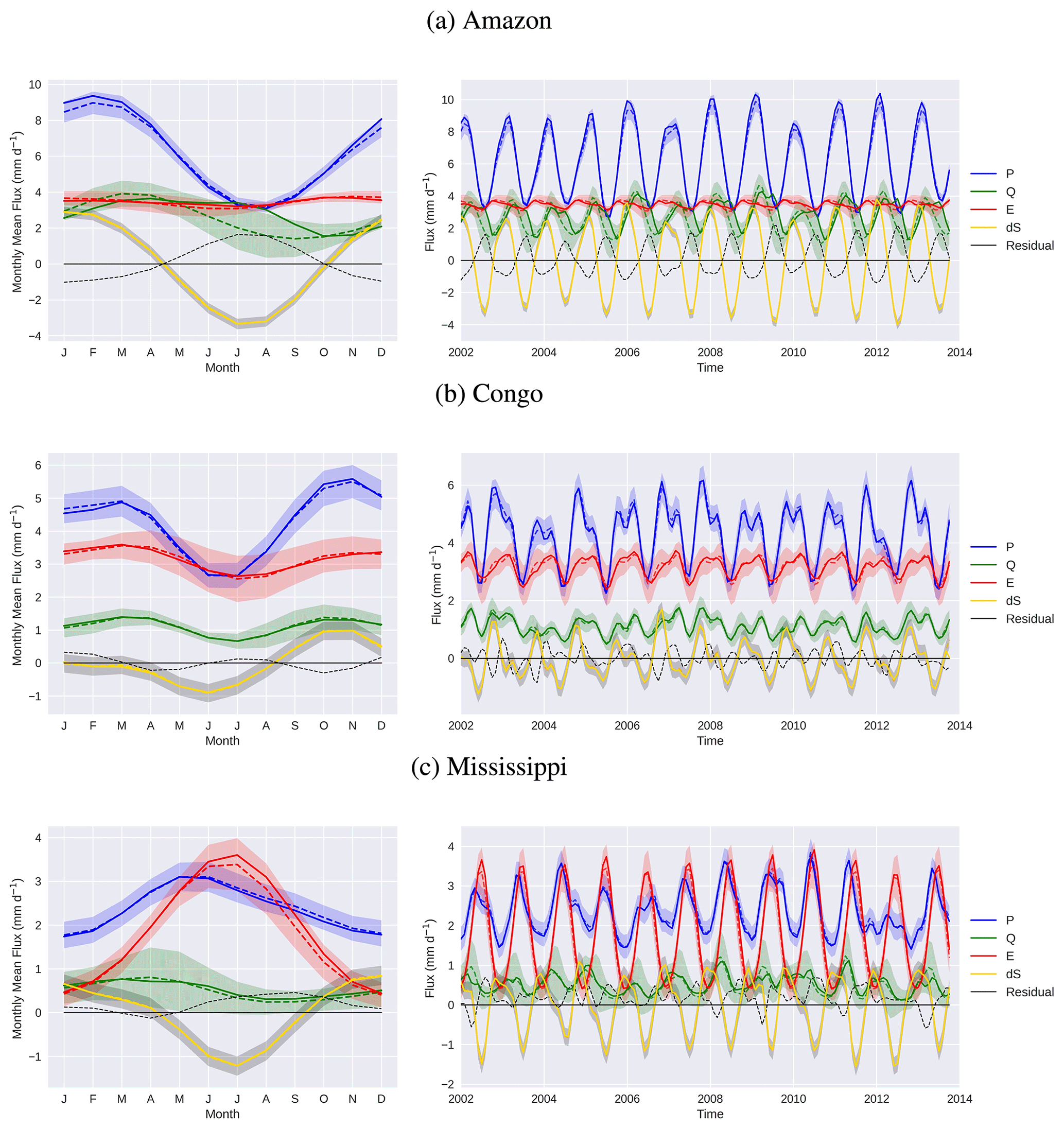
Figure 4Water budget fluxes. Observed values are shown by the dashed lines, and optimised values from our study are shown by the solid lines. The shaded regions show uncertainty in the observed values. Observed fluxes and derived products shown here (and the plots in the figures that follow) are all temporally smoothed, as described in Sect. 3.2.4. Mean seasonal cycles are shown on the left.
Over the Amazon, the seasonal cycle in precipitation largely converts directly into storage variations, with a smaller seasonal runoff signal lagging by around 3 months, reflecting the large basin size and slow runoff. Evaporation is almost constant through the year, reflecting the constantly moist rainforest conditions, with the very small adjustments making E even more uniform. The residual in the water budget also shows a regular seasonal cycle but is anti-correlated to precipitation. The optimisation acts to increased P and decreased Q from November–March when precipitation peaks, while the adjustment is mainly an increase in Q from June–August, which has the effect of prolonging the runoff peak, where the adjustment occasionally exceeds 1 SD. For these months, there are lower uncertainties for P and E; hence, most of the residual has been distributed to Q.
The Congo's precipitation is characterised by biannual peaks as the Intertropical Convergence Zone (ITCZ) migrates across the Equator. The primary maxima occur towards the end of the year, and the secondary maxima occur in May. The bimodal peaks are also seen in the Q and E fluxes. There is also considerable inter-annual variability in the precipitation. The small optimisation adjustments are not easily summarised in a regular seasonal pattern.
Unlike the other two basins, over the Mississippi the storage changes are almost out of phase with the precipitation. This reflects the dominance of storage in snow as a key controlling mechanism. The maximum runoff then occurs before the peak precipitation, indicative of snowmelt followed by early summer rains. Much of the seasonal precipitation peak is balanced by evaporation, which exceeds precipitation in July and also coincides with the largest reductions in storage. There are some very low precipitation years, such as 2006 and 2012. Due to the larger role of evaporation in this basin, the optimisation also shows a consistent E increase from July–December in each year. We will look at this in more detail when considering the coupling to the energy budget.
It can be seen that monthly adjustments remain small relative to the uncertainties, and these flux products are not therefore being independently validated on these timescales. Any validation of our products would require comparison with independent data that could be regarded as less uncertain than the datasets we have used. However, the benefit of our approach is shown over longer timescales below.
4.2 Total water storage
Greater insight into the fitting process and the changes involved are illustrated best by plotting the time history of surface water storage for a number of basins (Fig. 5). This quantity is very sensitive to flux imbalances, as small monthly imbalances accumulate and can cause unrealistic long-term storage changes. The left-hand plots show the GRACE storage target variability (in orange) and the flux-inferred storage (Sfi,w) from raw observations (dashed purple). For some basins, these already match reasonably well (e.g. Congo), but for others, the raw observations show large trends, and the (Sfi,w) disappears off the plot. Further details can be seen when looking at the () (solid purple). Here, the NET water fluxes have been detrended (D) to be consistent with the GRACE changes over the whole period but are otherwise unaltered, which allows the plot to show differences in the seasonal storage cycles. Over the Amazon, it is clear that the seasonal storage cycle from the original fluxes is too weak when compared with GRACE. Over the Amur, the flux-derived seasonal cycle is, in contrast, too large compared to GRACE. Several of the basins also show significantly different inter-annual variability. A larger set of basin imbalances can be seen in Fig. A1.
The plots on the right show that the storages based on the optimised fluxes (our Optimised Storage) now sit very clearly on top of the GRACE storage anomaly data, fitting both seasonal amplitudes and inter-annual variability in all basins very well. The storage differences compared to GRACE data are also shown, and these are always smaller than the 1 SD uncertainties applied to GRACE during optimisation. The associated optimised fluxes in Fig. 4 are also consistently within the uncertainty limits of the original flux data and therefore can be considered an improved, GRACE-consistent, product for describing water cycle variability on both short and longer timescales.

Figure 5GRACE storage compared with flux-inferred storage. On the left is the unadjusted Sfi,w (dashed red line) and the detrended (solid purple line), which is generated directly from observed fluxes. On the right, the “Optimised Storage”, based on the new fluxes from our study, is seen to closely follow the GRACE storage, which is shown in orange on the same axes in both plots.
4.3 Storage comparison with other products
We found that the total water storage anomaly is also a useful metric to compare against other products from the literature because it brings out low-frequency variations that would not be seen by comparing monthly fluxes, which will all lie within the uncertainty bounds of each other. We take the monthly water storage change products from three different recent budget closure studies and calculate the total water storage anomaly that these imply. The CLASS product (Hobeichi et al., 2020) provides a complete set of balanced coupled water and energy budget components on a global grid for the period 2003–2009, and we will later also compare with the energy budget from this solution. The CDR (Zhang et al., 2018), provides grid point estimates of monthly closed water budget components from 1984–2010, which includes a GRACE constraint over the later period. The REESEN product (Abolafia-Rosenzweig et al., 2021) used three different closure methods, and for this comparison, we take the ensemble mean from the combined proportional distribution (PR) method, which was described to give the best results. Each of these three products consists of optimised estimates which are consistent with GRACE on a monthly timescale, but in this section, we aim to assess consistency with GRACE over longer timescales. Hence, we do not show a comparison of monthly P, E, and Q fluxes but rather show the storage anomalies inferred from the fluxes.
We calculate the total water storage anomaly for the period 2003–2009, based on the overlap of these three products, and plot these against GRACE and our optimised solution in Fig. 6. Each storage has been initialised with GRACE for January 2003. It is clear that, while the other products have quite similar storage variability over each year, they all show some degree of divergence from GRACE storage over longer timescales. In the corrected REESEN dataset, mean product corrections show that the closure constraints act to increase observed by around 3 m per month on average. This adjustment may result in an upward trend in storage not observed by GRACE in some regions. For example, the REESEN product shows an upward storage trend over the Mississippi and Huang He basins, although over the Congo the storage fits GRACE quite well. The CLASS product shows an upward trend in water storage in all three basins and therefore shows storage differences at the end, reaching 14 cm equivalent over the Congo. The CDR product probably does best in fitting the 7-year trends for all three basins, as a long period water balancing correction is applied (Zhang et al., 2018); however, it shows anomalously weak seasonal variability in some years over the Mississippi and the Huang He and also misses some of the inter-annual variability over the Congo. The constraint we apply of fitting GRACE storage on all timescales can again be clearly seen. Although these other studies may have used different versions of the GRACE product as constraints, after comparison, we find that all GRACE products are very similar, and the differences shown here are coming from the optimisation approach.
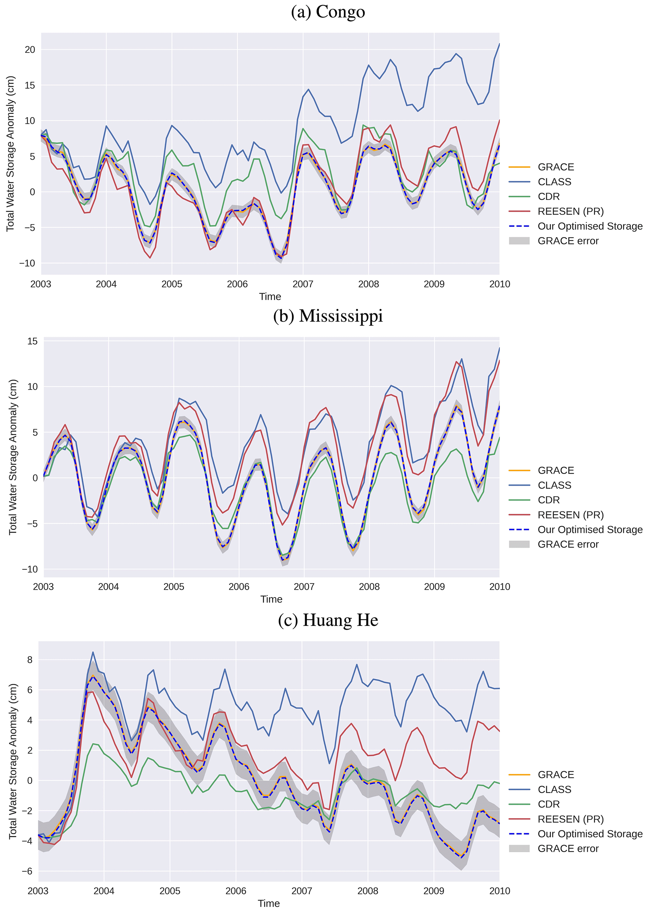
Figure 6Water storage product comparisons from 2003–2009 inclusive. The “Optimised Storage” line is the result from our study.
For the Mississippi, the CDR shows good agreement with GRACE, although it shows reduced seasonal cycles after 2008. CLASS and REESEN show a slightly positive bias compared to GRACE after 2005 but generally agree well with the size of the seasonal cycle. Over the Huang He, GRACE shows a large peak in water storage, followed by a decrease in storage, amounting to around 10 cm of water loss by 2009 (since the peak in 2003). All products capture the initial peak to some extent but fail to detect the downwards trend. The inter-annual variability in the seasonal cycle observed by GRACE is represented well by the REESEN product (such as the reduced seasonal cycle between 2006 and 2007 and the larger seasonal cycle in 2003). The timing of the seasonal cycle also shows good agreement. REESEN is able to detect the decline in storage 2004–2007 well; however, it does not capture the decline during 2008–2009. The CLASS product does not show good agreement with the overall trend in water storage. By 2009, there is over 6 cm difference between GRACE and the CLASS storage, since the downwards trend of GRACE was neither captured nor accounted for. The CDR consistently shows reduced seasonal cycles. Some of the inter-annual variability is captured, but it does not agree with the long-term trend. Since the CDR imposes a constraint which ensures dS=0 over 1984–2010, it means that the storage in 2010 must be the same as 1984, hence limiting the ability to detect trends.
Overall, from Fig. 6 we can conclude that although each of the other products are consistent with GRACE on a monthly timescale, all products show inconsistencies with GRACE storage anomalies on longer timescales, whereas our optimisation approach is able to guarantee consistency on all timescales.
4.4 Energy fluxes
The optimised energy components in Fig. 7 show only small differences from the observed fluxes used as input, although the long-term NET energy budget is now closed through the constraint coming from . To see the adjustments more clearly, Fig. 8 shows the seasonal mean adjustments to the NET downward flux and the component fluxes in three of the basins. The energy closure clearly requires a reduction in the NET downward energy flux in each of these basins in all months. Most flux components contribute fairly uniformly to the NET change, except for some variations responding to LE adjustments imposed through the water cycle. In all three basins, the adjustments to LE modulate NET changes through the year. In both the Amazon and the Mississippi, the adjustments through the water cycle are having a small dampening effect on the seasonal cycle in NET flux, as can be seen in Fig. 7. If any independent data on monthly NET flux or storage were to be available, then this would potentially change these monthly flux adjustments considerably, as we will discuss later.
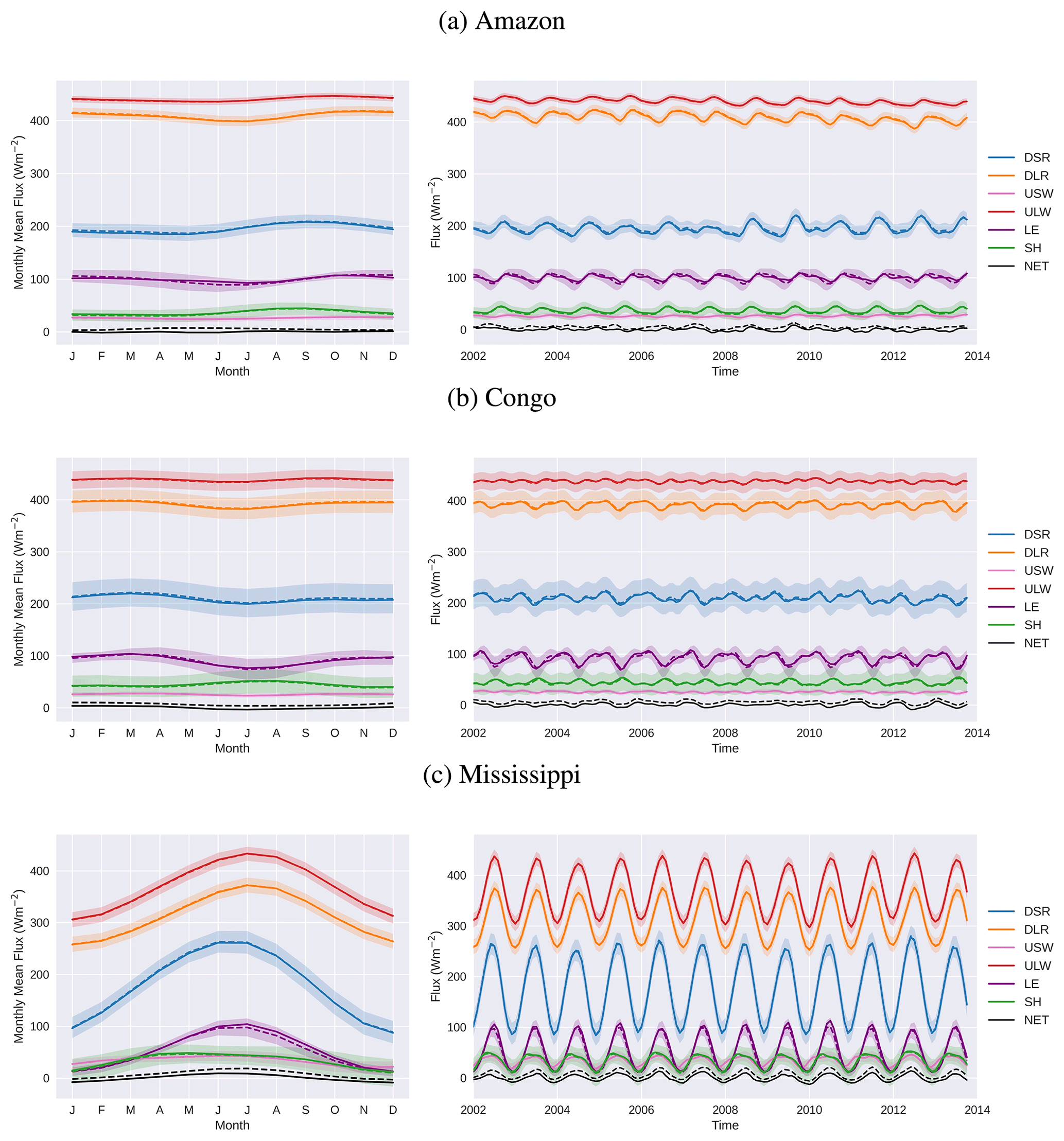
Figure 7Energy budget fluxes. Observed values are shown by the dashed lines and optimised values are shown by the solid lines. The shaded regions show uncertainty in the observed values. Mean seasonal cycles are shown on the left.
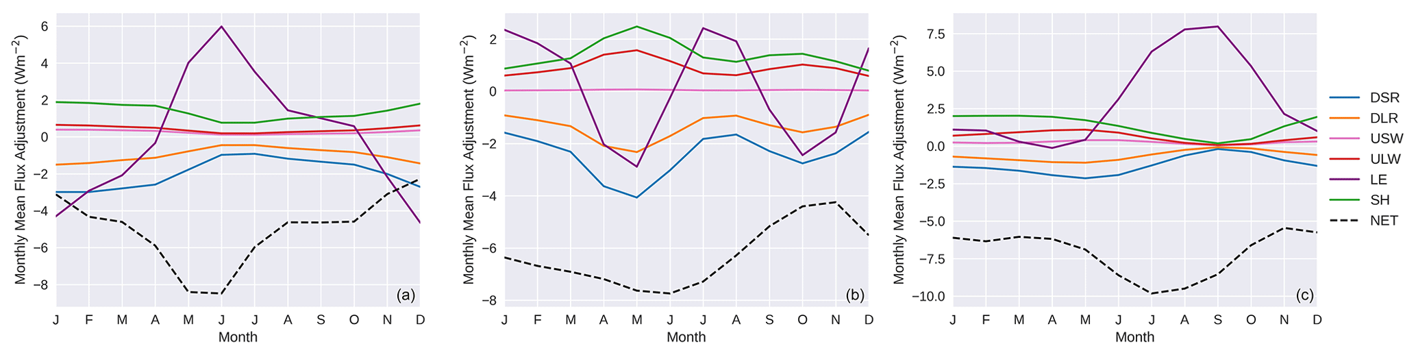
Figure 8Optimisation adjustments for the energy components. Optimised values minus observed values are shown for the Amazon (a), Congo (b), and Mississippi (c) river basins.
4.5 Total energy storage
Total energy storage anomalies are used to demonstrate the impact of our long-term constraint. We found, similar to the case for water storage, that this is a useful metric because small imbalances are not apparent when looking the monthly NET fluxes. But over longer periods, these small imbalances can be significant, which is captured by the total energy storage metric. For comparison, we use results from the CLASS product (Hobeichi et al., 2020), which is the only other study to provide coupled regional water and energy budgets at a monthly timescale. We compare both the inter-annual NET ground heat flux and the implied surface energy storage for several basins in Fig. 9. The assessment period covers January 2003 to December 2009, which is the time frame used in the CLASS study. The energy storage plots (Fig. 9, right) include the Sfi,e before the fluxes were detrended, in addition to our optimised solution and the CLASS solution. One key difference between our optimisation method and the method used in CLASS is that CLASS enforces monthly closure by using estimates of ground heat flux (equivalent to NET) as input, whereas, in our optimisation, we choose only to implement a long-term closure constraint which avoids using ground heat flux observations as input.
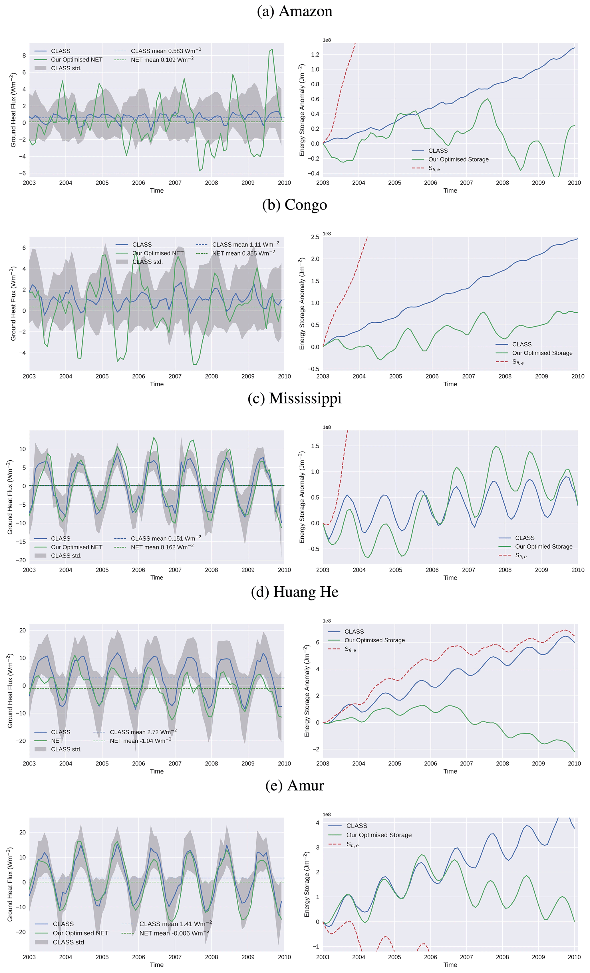
Figure 9NET fluxes (left) and total energy storage Sfi,e anomalies (right) during 2003–2009. The CLASS solutions are compared with our optimised solutions, with the Sfi,e also shown prior to optimisation (right).
In all basins, our initial NET energy fluxes are unbalanced and result in a strong storage trend (also seen in a wider range of basins in Fig. A2). The CLASS solutions also show smaller, but still potentially unrealistic, energy storage trends in all basins, apart from the Mississippi, because CLASS does not account for energy imbalances on timescales longer than 1 month. Both CLASS and our optimised fluxes show clear seasonal cycles of warming and cooling in the mid-latitude basins of the Mississippi, Amur, and Huang He rivers. There is much more variability in our NET fluxes, while the CLASS fluxes are similar every year, presumably reflecting the dampening effect of a ground heat flux constraint in CLASS. Our optimised solutions show more inter-annual flux and storage variability than CLASS, although this does not amount to any trend when the time series are extended to 2013 (over which time we have used the detrending energy constraint). This inter-annual variability is inherent in the initial energy fluxes, in particular from the radiation components, and is not in general being introduced through water cycle coupling. We will return to discuss this seasonal and inter-annual energy storage variability later.
5.1 Goodness of fit
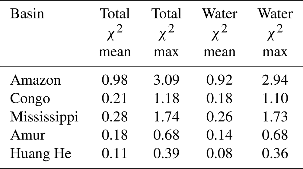
The χ2 values are summarised in Table 2. Each month, the four water variables expressed in Eq. (1) are required to balance. Although the energy budget in Eq. (2) is coupled and must also balance in the long-term, without an independent constraint on the NET monthly flux or energy storage change, these variables contribute very little to χ2, and the total χ2 values are only marginally larger than the water-only values. It can be seen that the average values are always much lower than 4 and remain smaller for the maximum value in any individual month. We conclude that all the sequential optimisations are providing solutions that are consistent and well within the given uncertainties.
Table 2The χ2 values for the optimisation include the total values, including all the water and energy flux terms, and with only the four water adjustment terms which are more strongly constrained at monthly timescales. The time mean χ2 over all months and the largest value for any individual month are also shown.
5.2 Uncertainty estimates
By using multiple datasets to constrain each other through budget closure, the uncertainty for the optimised estimates will be less than the uncertainty for the raw observations. The uncertainties for the new estimates are calculated using the same methods as the NEWS study, given by , where K is the Jacobian of R with respect to F, and SR is the uncertainty for the residual constraint R=0. Since we use a strong constraint to impose budget closure, the uncertainty SR is small. The uncertainties in the water budget terms before and after optimisation are shown in Table 3.
Table 3Average monthly water budget component uncertainties (mm d−1) before (obs) and after the optimisation.

It can be seen that uncertainties typically reduce by 10 % for precipitation but by substantially larger amounts for runoff and evaporation, where initial errors are larger. The uncertainties in storage change are only marginally affected. Of course, formally, post-optimisation uncertainties are correlated to reflect a closed water budget with no residual.
The initial imbalances in the water and energy budgets vary by basin. We found water budget residuals ranging between 1.5 % and 35 % of precipitation, which is comparable to Abolafia-Rosenzweig et al. (2021), who found that residual errors varied between 0.7 % and 30 % of precipitation. These initial imbalances are dependent on the quality of the input data, which differ according to the geophysical characteristics of the basins.
The Amazon has the largest absolute water budget residual prior to optimisation, averaging 0.86 mm d−1, which is equivalent to 14 % when expressed as a percentage of precipitation. Sahoo et al. (2011) also identified the Amazon as having the largest non-closure error and suggested that this could be as a result of the sparseness of in situ precipitation measurements over the basin which are required for the calibration of satellite estimates. The Congo showed the lowest initial imbalance of these basins, normalised with respect to P, with a monthly average of 6 %. However, this result is not necessarily due to good measurement coverage in this region. Low water budget residuals can also occur from the cancellation of errors or other characteristics of the basin. Further investigation would be required to better understand the factors determining these imbalances.
The similarities in our results compared to previous budget studies emphasise that our adjustments are of a similar size to other studies and within the observational errors. However, our results achieve an improved long-term consistency for water storage changes with GRACE, and therein lies the difference in our results. In previous budget closure studies, longer timescale constraints on the water budget have often been applied (e.g. Abolafia-Rosenzweig et al., 2021; Hobeichi et al., 2020), or generalised assumptions about total water storage anomalies have been made (Zhang et al., 2018). This can result in substantial misfits against the GRACE storage time series, particularly for regions which show significant trends and inter-annual variability. These previous studies have failed to match the low-frequency variations in GRACE storage anomalies, which are important to understand through hydrological modelling. The sequential optimisation approach used here is beneficial, as it enables to be constrained by GRACE on all timescales and guarantees that the total water storage anomaly implied from the optimised fluxes will track the inter-annual variability in GRACE, in addition to avoiding any unrealistic trends.
However, the sequential solution method does not permit flux adjustments across more than 1 month at a time. It is possible to make a whole period adjustment by closing the water budget every month while imposing a small or zero trend in the water storage from beginning to end of the time series. This would allow adjustments across months to fit longer-term changes, and this has been used for solving the seasonal cycle in the NEWS solution of Rodell et al. (2015), for example. However, this still does not guarantee a fit to the inter-annual variability information present in the GRACE time series. We made some comparisons, optimising for all months together (results not shown), and this worked well for some basins (e.g. Mississippi) and is then very similar to the sequential solution results, but it works much less well for other basins (e.g. Congo) when inter-annual variations are seen in the GRACE time series.
Our method also allows the optimised energy fluxes to be in good agreement with the initial energy flux observations, while also balancing the monthly water budget and removing long-term energy trends. However, the lack of a monthly NET energy constraint means that the energy budget is only very weakly constrained on short timescales. Further observational information, such as land surface temperatures, along with a heat capacity, could be used to constrain the energy storage on these timescales. Liu et al. (2017) propose NET heat flux estimates from ECMWF reanalyses, based on surface temperatures and some land surface modelling. Alternatively, some estimate of monthly NET ground heat flux upscaled from flux tower measurements could be imposed, as in Hobeichi et al. (2020). While we made some comparisons here, we have preferred to leave the monthly energy budget fairly unconstrained, as other monthly NET energy flux products have not been adequately validated for use as independent data. This also allows the surface variability inferred from other flux products to be clearly seen, such as in Fig. 9.
We have noted above that the differences between our NET energy fluxes and those reported by the CLASS product are likely due to the CLASS product including a ground heat flux product, G, in its formulation. G is the least well observed of all the energy balance fluxes, with typical measurements covering only very small areas. Consequently, large-scale gridded products tend to contain high levels of uncertainty due to errors in the representativity in the underlying data and hence rely on modelling assumptions that can have a strong influence on the resulting flux estimates. Consequently, we chose not to include a dataset of G in our budget modelling.
The results shown have all assumed that the initial errors are uncorrelated. However, due to the procedures required to derive some of the flux products, it is likely that not all fluxes are fully independent. For example, the GRUN product partly predicts runoff based on antecedent precipitation conditions, and so any error in P may also be present in Q. Specifying an error covariance (off-diagonal elements in Eq. 11) impacts how the fluxes are adjusted during the optimisation and also reduces the effective number of independent variables. We performed some sensitivity tests, applying error covariances through the covariance matrix (Sobs). To give an example, consider the P and Q errors to be correlated. Adjustments needed to close the water budget in Eq. (1) would normally require P and Q to be adjusted in opposite directions; for example, a smaller P and larger Q would both reduce a positive budget residual. However, correlated P and Q errors would tend to inhibit an opposite adjustment of this sort. As a consequence, imposing correlated P and Q errors will lead to smaller adjustments in both P and Q and require the other budget terms, E and , to have larger adjustments in order to close the budget. This is demonstrated in Sect. 4.
The same arguments apply for correlated errors in the energy fluxes. If upward and downward radiation flux errors are positively correlated, then this will reduce the degrees of freedom, reduce the adjustments in those fluxes, and increase budget balancing adjustments to other fluxes. Correlating sensible and latent flux errors (both upward fluxes), however, as implied by eddy covariance studies, e.g. Twine et al. (2000), will increase their adjustment contributions by reducing their joint cost function impacts. As all adjustments we found were well within error bounds in these regional solutions, we did not find any inconsistencies when imposing realistically correlated initial errors. However, it is worth commenting that if flux component error correlations are present, then they may be quite pervasive and would then imply larger or smaller adjustments to large-scale energy fluxes. This would end up changing, for example, the relative adjustments to radiation compared with turbulent fluxes in global inverse budgets (as described in L'Ecuyer et al., 2015).
This study has introduced a sequential optimisation approach which is used to produce coupled estimates for the components of the terrestrial water and energy budgets based on observations. The focus has been on several large river basins over the period 2002 to 2013. The optimisation approach differs from other studies which have used GRACE to constrain hydrological models, as it acts to close the monthly water budget while at the same time matching the water budget on longer timescales. This then achieves a good fit with the GRACE surface water storage time series in each basin when the optimised fluxes are integrated, whereas previous studies have failed to match low-frequency variations in GRACE, which are important to understand through hydrological modelling. The coupled energy budget is also solved sequentially, while still guaranteeing a long-term energy balance. This is achieved using a detrended monthly energy storage target , based on the original fluxes, as a weak constraint. Solving for the water and energy budgets simultaneously has allowed us to provide more observational constraints and ensure consistency in our final estimates, which has only been done in a limited number of studies. All the flux adjustments made during the optimisation are small and within uncertainty estimates, and the inter-annual variability from observations is retained. The optimisation also has the benefit of reducing formal uncertainties for the individual flux components.
We produce Sfi by using the observed fluxes in and out of a region to infer the water and energy storage over time. This gives a sensitive measure of the imbalances, seasonal cycles, and inter-annual variability amplitudes implied by the fluxes that can then also be compared with GRACE and with several other products from the literature. For several basins, the input water fluxes show weaker or stronger seasonal amplitudes than suggested by GRACE, which are then corrected during the optimisations.
The current study has focused on methods for budget-balancing adjustments. We have not used a selection of different input data products to test the relative imbalance from different choices. Also budgets are only balanced on a selection of larger land hydrological basins. Figures relevant to more basins are included in the Appendix. We have not produced a gridded product of optimised fields, although this could be done at some resolution consistent with the resolution of the input products, in particular the GRACE data.
Although the energy budget is coupled, the current solutions are only constrained on long timescales. Flux components adjust to a long-term surface energy balance, accounting for any mean changes in latent losses imposed through the water cycle; otherwise, monthly energy components are relatively unconstrained. Further work could seek to constrain the surface energy fluxes on shorter timescales by introducing additional energy storage data, e.g. using land surface temperatures either from EO or reanalysis products (Liu et al., 2017).
Another direction of work could seek to include a coupled water and energy budget for the atmosphere. This could be built into a global solution, as in NEWS (Rodell et al., 2015; L'Ecuyer et al., 2015), or else would need to include regional boundary transport estimates in the atmosphere for both energy and water (Mayer et al., 2022).
Overall, this study has presented a methodological advancement in fully utilising the GRACE water storage observations to constrain regional water fluxes from monthly to decadal timescales. The constraints imposed as part of this study and the direction of future work are aimed at improving the accuracy of water and energy cycle components, which can ultimately help us gain a better understanding of climate processes and improve the skill of climate models in predicting future change.
The following figures illustrate the results for a wider selection of basins across the globe, with varying initial imbalances.
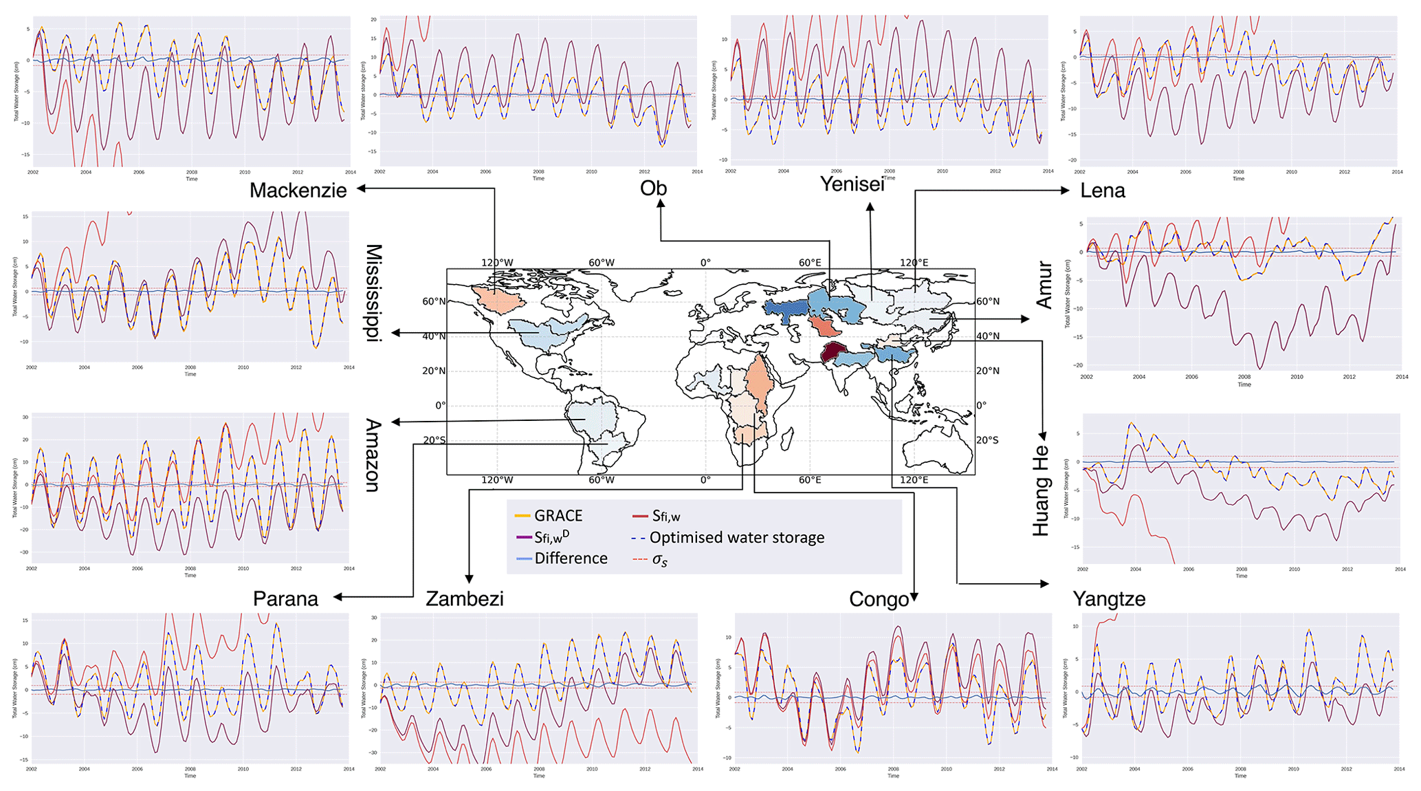
Figure A1Monthly water storage variability in a selection of basins for January 2002–October 2013. GRACE data are shown (orange), with the optimised water storage solution (dashed blue) overlaying it closely. The optimised differences to GRACE are also shown along with the GRACE uncertainties, σS, varying near 0. The figure also shows two versions of flux-inferred storage (Sfi,w) from the input data. The original Sfi,w (red) is the storage implied by integrating the input () in time. This often diverges rapidly, demonstrating strong initial imbalances (the basins are coloured according to this initial imbalance). The detrended (mauve) simply detrends those original fluxes to fit the mean GRACE storage trend. This reveals interesting details about the initial mismatch between water fluxes and GRACE, for example, by showing an underestimate in seasonal in the Amazon and a strong overestimate in seasonal storage in the high-latitude rivers. Many basins also show mismatches in the inter-annual variations compared to GRACE, which are all removed in the optimisation process.

Figure A2Monthly surface energy storage variability in a selection of basins for January 2002–October 2013. The original flux-inferred storage Sfi,e (in red) is the storage implied by integrating the input (NET) in time. This always diverges rapidly, demonstrating strong initial energy imbalances (the basin map is coloured according to these initial imbalances). The detrended (green line) simply detrends the original NET flux to give a 0 energy storage trend. This retains the details of both the seasonal and inter-annual surface energy variability. The implied inter-annual variability in surface storage is large compared to seasonal variations and can mostly be traced to variations in surface radiation fields. Such inter-annual variability may be unrealistic, but without the reliable observations of ground NET heat flux or a measure of surface storage (e.g. from land surface temperatures), we have chosen to retain it during optimisation (see the text for details). The optimised energy storage is also shown (dashed blue), and this broadly tracks the , which is used as a monthly constraint. Any divergence is confined to the first few months so that the energy budget is closely balanced throughout the period. The difference in the optimised storage is also shown, along with the large uncertainty limits used σe (see text for details).
The observational data used as input are available from several different sources. GRUNv1 runoff data can be obtained from https://www.bafg.de/GRDC/EN/04_spcldtbss/43_GRfN/refDataset_node.html (GRDC, 2020), GPCPv2.3 precipitation data can be obtained from https://doi.org/10.7289/V56971M6 (Adler et al., 2016b), turbulent heat flux data from FLUXCOM can be obtained from https://doi.org/10.17871/FLUXCOM_EnergyFluxes_v1 (Jung, 2018), and CERES radiative flux data are available at https://ceres-tool.larc.nasa.gov/ord-tool/jsp/EBAFTOA42Selection.jsp (Loeb et al., 2018). The CLASS product used as comparison in this study is available from https://doi.org/10.25914/5c872258dc183 (Hobeichi et al., 2019), and the REESEN and basin-scale CDR products are archived on Mendeley Data and available at https://doi.org/10.17632/r24rdxt73j.3 (Abolafia-Rosenzweig and Livneh, 2020).
The optimisation code developed in this study and optimised data for several basins are available at https://doi.org/10.5281/zenodo.7682197 (Petch, 2023). Data for additional basins can be made available upon request to the corresponding author.
This work was carried out by SP, initially as part of her Masters degree and subsequently as a contribution to her doctoral degree. All the analysis and figures were generated by SP, in addition to a first draft of the text. KH, TQ, and RK acted as supervisors for SP's doctorate, and BD helped with data acquisition and analysis. All co-authors contributed edits to the text.
The contact author has declared that none of the authors has any competing interests.
Publisher's note: Copernicus Publications remains neutral with regard to jurisdictional claims in published maps and institutional affiliations.
This work was performed as part of the PhD project of Samantha Petch.
This research has been supported by the NERC DTP SCENARIO programme and NERC NCEO International Programme (grant no. NE/X006328/1).
This paper was edited by Hubert H. G. Savenije and reviewed by three anonymous referees.
Abolafia-Rosenzweig, R. and Livneh, B.: Remotely sensed ensemble of the water cycle, Mendeley Data [data set], https://doi.org/10.17632/r24rdxt73j.3, 2020. a
Abolafia-Rosenzweig, R., Pan, M., Zeng, J., and Livneh, B.: Remotely sensed ensembles of the terrestrial water budget over major global river basins: An assessment of three closure techniques, Remote Sens. Environ., 252, 112191, https://doi.org/10.1016/j.rse.2020.112191, 2021. a, b, c, d, e, f, g, h
Acker, J., Williams, R., Chiu, L., Ardanuy, P., Miller, S., Schueler, C., Vachon, P., and Manore, M.: Remote Sensing from Satellites, in: Reference Module in Earth Systems and Environmental Sciences, Elsevier, https://doi.org/10.1016/B978-0-12-409548-9.09440-9, 2014. a
Adler, R. F., Huffman, G. J., Chang, A., Ferraro, R., Xie, P., Janowiak, J., Rudolf, B., Schneider, U., Curtis, S., Bolvin, D., Gruber, A., Susskind, J., P. Arkin, P., and Nelkin, E.: The version-2 Global Precipitation Climatology Project (GPCP) monthly precipitation analysis (1979–present), J. Hydrometeorol., 4, 1147–1167, https://doi.org/10.1175/1525-7541(2003)004<1147:TVGPCP>2.0.CO;2, 2003. a, b
Adler, R., Huffman, G., Arkin, P., Chang, A., Ferraro, R., Gruber, A., Janowiak, J., McNab, A., Rudolf, B., and Schneider, U.: An Update (Version 2.3) of the GPCP Monthly Analysis, B. Am. Meteorol. Soc., 78, 5–20, 2016a. a, b, c
Adler, R., Wang, J.-J., Sapiano, M., Huffman, G., Chiu, L., Xie, P. P., Ferraro, R., Schneider, U., Becker, A., Bolvin, D., Nelkin, E., Gu, G., and NOAA CDR Program: Global Precipitation Climatology Project (GPCP) Climate Data Record (CDR), Version 2.3 (Monthly), National Centers for Environmental Information [data set], https://doi.org/10.7289/V56971M6, 2016b. a
Aires, F.: Combining Datasets of Satellite-Retrieved Products. Part I: Methodology and Water Budget Closure, J. Hydrometeorol., 15, 1677–1691, https://doi.org/10.1175/JHM-D-13-0148.1, 2014. a, b
Chen, J., Tapley, B., Rodell, M., Seo, K., Wilson, C., Scanlon, B., and Pokhrel, Y.: Basin-Scale River Runoff Estimation from GRACE Gravity Satellites, Climate Models and In Situ Observations: a Case Study in the Amazon Basin, Water Resour. Res., 56, e2020WR028032, https://doi.org/10.1029/2020WR028032, 2020. a, b
Do, H. X., Gudmundsson, L., Leonard, M., and Westra, S.: The Global Streamflow Indices and Metadata Archive (GSIM) – Part 1: The production of a daily streamflow archive and metadata, Earth Syst. Sci. Data., 10, 765–785, https://doi.org/10.5194/essd-10-765-2018, 2018. a
Dong, B., Lenters, J. D., Hu, Q., Kucharik, C. J., Wang, T., Soylu, M. E., and Mykleby, P. M.: Decadal-Scale Changes in the Seasonal Surface Water Balance of the Central United States from 1984 to 2007, J. Hydrometeorol., 21, 1905–1927, 2020. a
Eicker, A., Forootan, E., Springer, A., and Longuevergne, L.: Supporting Information for “Does GRACE see the terrestrial water cycle intensifying”?, J. Geophys. Res., 121, 733–745, https://doi.org/10.1002/2015JD023808, 2015. a, b
FluxCom: Energy fluxes, http://fluxcom.org/, last access: 28 July 2021. a
Ghiggi, G., Humphrey, V., Seneviratne, S. I., and Gudmundsson, L.: GRUN: an observation-based global gridded runoff dataset from 1902 to 2014, Earth Syst. Sci. Data, 11, 1655–1674, https://doi.org/10.5194/essd-11-1655-2019, 2019. a, b, c
GravIS: Gravity Information Service: Terrestrial water storage anomalies, Helmholtz Centre, Potsdam, http://gravis.gfz-potsdam.de/land, last access: 1 August 2021. a
GRDC: GRDC Reference Dataset, GRDC [data set], https://www.bafg.de/GRDC/EN/04_spcldtbss/43_GRfN/refDataset_node.html (last access: 31 October 2019), 2020. a, b
Hobeichi, S., Abramowitz, G., and Evans, J.: Conserving Land-Atmosphere Synthesis Suite (CLASS) v 1.1 (2019), NCI Data Catalogue [data set], https://doi.org/10.25914/5c872258dc183, 2019. a
Hobeichi, S., Abramowitz, G., and Evans, J.: Conserving Land–Atmosphere Synthesis Suite (CLASS), J. Climate, 33, 1821–1855, 2020. a, b, c, d, e, f, g, h, i, j, k
IPCC: Intergovernmental Panel on Climate Change: The physical science basis, in: Working Group I contribution to the IPCC Fifth Assessment Report, Cambridge University Press, Cambridge, UK, https://www.ipcc.ch/report/ar5/wg1/ (last access: 12 October 2022), 2013. a
Jung, M.: FLUXCOM Global Land Energy Fluxes, FluxCom Data Portal [data set], https://doi.org/10.17871/FLUXCOM_EnergyFluxes_v1, 2018. a
Jung, M., Koirala, S., Weber, U., and Coauthors: The FLUXCOM ensemble of global land-atmosphere energy fluxes, Sci. Data, 6, 74, https://doi.org/10.1038/s41597-019-0076-8, 2019. a, b, c
Kato, S., Rose, F. G., Rutan, D. A., Thorsen, T. E., Loeb, N. G., Doelling, D. R., Huang, X., Smith, W. L., S, W., and Ham, S.-H.: Surface irradiances of Edition 4.0 Clouds and the Earth's Radiant Energy System (CERES) Energy Balanced and Filled (EBAF) data product, J. Climate, 31, 4501–4527, https://doi.org/10.1175/JCLI-D-17-0523.1, 2018. a
Kim, H., Watanabe, S., Chang, E. C., Yoshimura, K., Hirabayashi, J., Famiglietti, J., and Oki, T.: Global Soil Wetness Project Phase 3 Atmospheric Boundary Conditions (Experiment 1), DIAS – Data set, Data Integration and Analysis System [data set], https://doi.org/10.20783/DIAS.501, 2017. a
Landerer, F. and Swenson, S.: Accuracy of scaled GRACE terrestrial water storage estimates, Water Resour. Res., 48, 1–11, 2012. a
L'Ecuyer, T., Beaudoing, H. K., Rodell, M., Olson, W., Lin, B., Kato, S., Clayson, C., Wood, E., Sheffield, J., Adler, R., Huffman, G., Bosilovich, M., Gu, G., Robertson, F., Houser, P. R., Chambers, D., Famiglietti, J. S., Fetzer, E., Liu, W. T., Gao, X., Schlosser, C., Clark, E., Lettenmaier, D. P., and Hilburn, K.: The Observed State of the Energy Budget in the Early Twenty-First Century, J. Climate, 28, 8319–8346, 2015. a, b, c, d, e, f
Lehmann, F., Vishwakarma, B. D., and Bamber, J.: How well are we able to close the water budget at the global scale?, Hydrol. Earth Syst. Sci., 26, 35–54, https://doi.org/10.5194/hess-26-35-2022, 2022. a, b
Liu, C., Allan, R. P., Mayer, M., Hyder, P., Loeb, N. G., Roberts, C. D., Valdivieso, M., Edwards, J. M., and Vidale, P.-L.: Evaluation of satellite and reanalysis-based global net surface energy flux and uncertainty estimates, J. Geophys. Res.-Atmos., 122, 6250–6272, https://doi.org/10.1002/2017JD026616, 2017. a, b
Loeb, N. G., Su, W., Doelling, D., Wong, T., Minnis, P., Thomas, S., and Miller, W.: Earth's top-of-atmosphere radiation budget, Comprehens. Remote Sens., 5, 67–84, https://doi.org/10.1016/B978-0-12-409548-9.10367-7, 2016. a
Loeb, N., Doelling, D., Wang, H., Su, W., Nguyen, C., Corbett, J., Liang, L., Mitrescu, C., Rose, F., and Kato, S.: Clouds and the Earth's Radiant Energy System (CERES) Energy Balanced and Filled (EBAF) Top-of-Atmosphere (TOA) Edition-4.0 Data Product (2018), NASA [data set], https://ceres-tool.larc.nasa.gov/ord-tool/jsp/EBAFTOA42Selection.jsp (last access: 18 February 2022), 2018. a
Long, D., Yang, Y., Wada, Y., Hong, Y., Liang, W., Chen, Y., Yong, B., Hou, A., Wei, J., and Chen, L.: Deriving scaling factors using a global hydrological model to restore GRACE total water storage changes for China's Yangtze River Basin, Remote Sens. Environ., 168, 177–193, 2015. a
Mayer, J., Mayer, M., Haimberger, L., and Liu., C.: Comparison of Surface Energy Fluxes from Global to Local Scale, J. Climate, 35, 4551–4569, 2022. a
Munier, S. and Aires, F.: A new global method of satellite dataset merging and quality characterization constrained by the terrestrial water budget, Remote Sens. Environ., 205, 19–130, 2018. a
Munier, S., Aires, F., Schlaffer, S., Prigent, C., Papa, F., Maisongrande, P., and Pan, M.: Combining data sets of satellite-retrieved products for basin-scale water balance study: 2. Evaluation on the Mississippi Basin and closure correction model, J. Geophys. Res.-Atmos., 119, 12100–12116, 2014. a, b
Pan, M., Sahoo, A., Troy, T., Vinukollu, R., Sheffield, J., and Wood, E.: Multisource Estimation of Long-Term Terrestrial Water Budget for Major Global River Basins, J. Climate, 25, 3191–3206, 2012. a, b, c
Pellet, V., Aires, F., Munier, S., Prieto, D., Jordá, G., Dorigo, W. A., Polcher, J., and Brocca, L.: Integrating multiple satellite observations into a coherent dataset to monitor the full water cycle – Application to the Mediterranean region, Hydrol. Earth Syst. Sci., 23, 465–491, https://doi.org/10.5194/hess-23-465-2019, 2019. a, b
Petch, S.: sammypetch/Water-and-energy-budgets: v2, Zenodo [code], https://doi.org/10.5281/zenodo.7682197, 2023. a
Reeves Eyre, J. and Zeng, X.: The Amazon Water Cycle: Perspectives from Water Budget Closure and Ocean Salinity, J. Climate, 34, 1439–1451, 2021. a, b
Rodell, M., McWilliams, E. B., Famiglietti, J. S., Beaudoing, H. K., and Nigro, J.: Estimating evapotranspiration using an observation based terrestrial water budget, Hydrol. Process., 25, 4082–4092, https://doi.org/10.1002/hyp.8369, 2011. a
Rodell, M., Beaudoing, H., L'Ecuyer, T., Olson, W., Famiglietti, J., Houser, P., Adler, R., Bosilovich, M., Clayson, C., Chambers, D., Clark, E., Fetzer, E., Gao, X., Gu, G., Hilburn, K., Huffman, G., Lettenmaier, D., Liu, W., Robertson, F., Schlosser, C., Sheffield, J., and Wood, E.: The observed state of the water cycle in the early twenty-first century, J. Climate, 28, 8289–8318, 2015. a, b, c, d, e
Rodell, M., Famiglietti, J. S., Wiese, D. N., Reager, J. T., Beaudoing, H. K., Landerer, F. W., and Lo, M.-H.: Emerging trends in global freshwater availability, Nature, 557, 651–659, 2018. a
Sahoo, A., Pan, M., Troy, T., Vinukollu, R., Sheffield, J., and Wood, E.: Reconciling the global terrestrial water budget using satellite remote sensing, Remote Sens. Environ., 115, 1850–1865, 2011. a, b, c
Sheffield, J., Ferguson, C., Troy, T., Wood, E., and McCabe, M.: Closing the terrestrial water budget from satellite remote sensing, Geophys. Res. Lett., 36, L07403, https://doi.org/10.1029/2009GL037338, 2009. a, b, c, d
Swenson, S. and Wahr, J.: Post-processing removal of correlated errors in GRACE data, Geophys. Res. Lett., 33, 8402, https://doi.org/10.1029/2005GL025285, 2006. a
Tapley, B. D., Watkins, M. M., Flechtner, F., Reigber, C., Bettadpur, S., Rodell, M., Sasgen, I., Famiglietti, J. S., Landerer, F. W., Chambers, D. P., Reager, J. T., Gardner, A. S., Save, H., Ivins, E. R., Swenson, S. C., Boening, C., Dahle, C., Wiese, D. N., Dobslaw, H., Tamisiea, M. E., and Velicogna, I.: Contributions of GRACE to understanding climate change, Nat. Clim. Change, 9, 358–369, https://doi.org/10.1038/s41558-019-0456-2, 2019. a
Thomas, C., Dong, B., and Haines, K.: Inverse modeling of global and regional energy and water cycle fluxes using earth observation data, J. Climate, 33, 1707–1723, 2020. a
Twine, T. E., Kustas, W. P., Norman, J. M., Cook, D. R., Houser, P. R., Meyers, T. P., Prueger, J. H., P. J, S., and Wesely, M. L.: Correcting eddy-covariance flux underestimates over a grassland, Agr. Forest Meteorol., 103, 279–300, https://doi.org/10.1016/S0168-1923(00)00123-4, 2000. a
Wang, S., Huang, J., Yang, D., Pavlic, G., and Li, J.: Long-term water budget imbalances and error sources for cold region drainage basins, Hydrol. Process., 29, 2125–2136, 2015. a, b
Warszawski, L., Frieler, K., Huber, V., Piontek, F., Serdeczny, O., and Schewe, J.: The Inter-Sectoral Impact Model Intercomparison Project (ISI–MIP): Project framework, P. Natl. Acad. Sci. USA, 111, 3228–3232, https://doi.org/10.1073/pnas.1312330110, 2014. a
Wielicki, B. A., Barkstrom, B. R., Harrison, E. F., Lee, R. B., Smith, G. L., and Cooper, J. E.: Clouds and the Earth's RadiantEnergy System (CERES): An Earth Observing System exper-iment, B. Am. Meteorol. Soc., 77, 853–868, 1996. a, b
Wiese, D., Landerer, F. W., and Watkins, M. M.: Quantifying and reducing leakage errors in the JPL RL05M GRACE mascon solution, Water Resour. Res., 52, 7490–7502, 2016. a, b, c, d
Zhang, Y., Pan, M., Sheffield, J., Siemann, A. L., Fisher, C. K., Liang, M., Beck, H. E., Wanders, N., MacCracken, R. F., Houser, P. R., Zhou, T., Lettenmaier, D. P., Pinker, R. T., Bytheway, J., Kummerow, C. D., and Wood, E. F.: A Climate Data Record (CDR) for the global terrestrial water budget: 1984–2010, Hydrol. Earth Syst. Sci., 22, 241–263, https://doi.org/10.5194/hess-22-241-2018, 2018. a, b, c, d, e, f, g, h, i