the Creative Commons Attribution 4.0 License.
the Creative Commons Attribution 4.0 License.
 | 14 Apr 2023
Diagnosing modeling errors in global terrestrial water storage interannual variability
Martin Jung
Nuno Carvalhais
Tina Trautmann
Basil Kraft
Markus Reichstein
Matthias Forkel
Sujan Koirala
Terrestrial water storage (TWS) is an integrative hydrological state that is key for our understanding of the global water cycle. The TWS observation from the GRACE missions has, therefore, been instrumental in the calibration and validation of hydrological models and understanding the variations in the hydrological storage. The models, however, still show significant uncertainties in reproducing observed TWS variations, especially for the interannual variability (IAV) at the global scale. Here, we diagnose the regions dominating the variance in globally integrated TWS IAV and the sources of the errors in two data-driven hydrological models that were calibrated against global TWS, snow water equivalent, evapotranspiration, and runoff data. We used (1) a parsimonious process-based hydrological model, the Strategies to INtegrate Data and BiogeochemicAl moDels (SINDBAD) framework and (2) a machine learning, physically based hybrid hydrological model (H2M) that combines a dynamic neural network with a water balance concept.
While both models agree with the Gravity Recovery and Climate Experiment (GRACE) that global TWS IAV is largely driven by the semi-arid regions of southern Africa, the Indian subcontinent and northern Australia, and the humid regions of northern South America and the Mekong River basin, the models still show errors such as the overestimation of the observed magnitude of TWS IAV at the global scale. Our analysis identifies modeling error hotspots of the global TWS IAV, mostly in the tropical regions including the Amazon, sub-Saharan regions, and Southeast Asia, indicating that the regions that dominate global TWS IAV are not necessarily the same as those that dominate the error in global TWS IAV. Excluding those error hotspot regions in the global integration yields large improvements in the simulated global TWS IAV, which implies that model improvements can focus on improving processes in these hotspot regions. Further analysis indicates that error hotspot regions are associated with lateral flow dynamics, including both sub-pixel moisture convergence and across-pixel lateral river flow, or with interactions between surface processes and groundwater. The association of model deficiencies with land processes that delay the TWS variation could, in part, explain why the models cannot represent the observed lagged response of TWS IAV to precipitation IAV in hotspot regions that manifest as errors in global TWS IAV. Our approach presents a general avenue to better diagnose model simulation errors for global data streams to guide efficient and focused model development for regions and processes that matter the most.
- Article
(19341 KB) - Full-text XML
- BibTeX
- EndNote


Terrestrial water storage (TWS) encompasses all storage of water over the land surface and in the subsurface, including groundwater, soil moisture, vegetation water, surface water, snow, and ice. As a major component of the global hydrological cycle, it controls the energy and biogeochemical fluxes (Famiglietti, 2004; Pokhrel et al., 2021). Furthermore, TWS is linked to occurrences of droughts, floods, and food production and human security over land (Tapley et al., 2019). In terms of processes, TWS buffers the drainage of precipitation and partly supports transpiration and vegetation photosynthesis during the dry season (Chapin et al., 2011; Guan et al., 2014; Madani et al., 2020; Miguez-Macho and Fan, 2021), which in turn affects the land–atmosphere feedbacks. Globally, TWS is associated with the rate or amount of carbon exchange between the land and atmosphere (e.g., Jung et al., 2017; Humphrey et al., 2018; Luo and Keenan, 2022; Wang et al., 2022). The TWS is, thus, a key variable for understanding the global energy, water, and carbon cycles and their interactions with climate change.
As TWS controls several mechanisms and processes over land, the TWS observations from the Gravity Recovery and Climate Experiment (GRACE) satellite missions, launched in March 2002, have been extremely valuable for understanding global hydrological processes and storage (e.g., Kim et al., 2009) and evaluating and improving hydrological models (e.g., Lo et al., 2010; Schellekens et al., 2017; Zhang et al., 2017; Trautmann et al., 2018). For example, GRACE TWS was used to study the effect of global climate change on sea level rise (e.g., Reager et al., 2016; Scanlon et al., 2018), estimate continental discharge using a data assimilation framework (e.g., Syed et al., 2009), predict floods (e.g., Reager and Famiglietti, 2009), and quantify the anthropogenic influence in the global hydrological cycle such as groundwater depletion (e.g., Rodell et al., 2009; Felfelani et al., 2017; Meghwal et al., 2019; Hosseini-Moghari et al., 2020; Liu et al., 2021) and dam construction (e.g., Awange et al., 2019). In relation to hydrological model evaluations and improvements, GRACE observations have been used to estimate model parameters and evaluate model simulations at regional (e.g., Lo et al., 2010), continental (e.g., Trautmann et al., 2018), and global (e.g., Kraft et al., 2022; Trautmann et al., 2022) scales. Constrained by GRACE observations, the uncertainties in model predictions are reduced, and the same model simulations have contributed to better understanding of the global TWS variations (e.g., Kraft et al., 2022; Trautmann et al., 2022). For instance, Trautmann et al. (2018) calibrated a process-based hydrological model with multiple observation products, including GRACE TWS, to show that snow dominates the mean seasonal TWS variability, while liquid water dominates the interannual TWS variability over northern mid-to-high latitudes.
Despite the advances in modeling TWS, the errors in TWS simulations are not fully understood and addressed. For example, Zhang et al. (2017) evaluated TWS estimates in four different global hydrological models against GRACE and revealed that the model performance varied significantly across basins, even within the same climate zone. Scanlon et al. (2018) also reported that TWS trends by global hydrological models were underestimated or had the opposite sign over basins across the globe, compared to GRACE-derived TWS trends. Particularly, a notable mismatch in TWS between models and GRACE is at the interannual temporal scale, which is relatively less understood compared to the long-term trend which has been extensively studied to quantify the impact of anthropogenic activities on the water cycle (e.g., Rodell et al., 2009; Scanlon et al., 2018; Meghwal et al., 2019). Studies have reported that global hydrological models performed relatively worse when reproducing observed global TWS interannual variability (IAV) compared to other temporal scales (e.g., Zhang et al., 2017; Kraft et al., 2022). Jensen et al. (2020) showed that the longer-term variability in TWS is dominant in GRACE compared to seasonal variations in Earth system models and suggested that the models are less reliable for reproducing the timing of peaks of TWS IAV across years, compared to the magnitude and frequency.
It is, nonetheless, imperative to understand the sources of modeling errors in the global TWS IAV, as they may lead to the misunderstanding of Earth's hydrological change, such as the trend of water availability (e.g., Jensen et al., 2019; Scanlon et al., 2018), extreme events such as droughts and floods (e.g., Chen et al., 2010; Humphrey et al., 2016), and even the observed global water–carbon interactions (e.g., Jung et al., 2017; Humphrey et al., 2018, 2021) and land–atmosphere–climate interactions (e.g., Jensen et al., 2019). Despite findings that the global TWS variability is dominated by the humid tropical regions (e.g., Syed et al., 2008, 2009; Humphrey et al., 2016), there are obstacles to understanding the global modeling errors and attributing them to regions or specific processes. The spatial pattern of errors largely varies among models and even varies with the climate zone for the same model (Zhang et al., 2017). In addition, hydrological mechanisms underlying the TWS IAV modeling error are relatively unclear due to differences in the modeling structure. As TWS variations emerge from complex water cycle dynamics and interactions among storage and water–carbon cycle linkages, the model errors may be due to different inherent assumptions and processes. Therefore, understanding the spatiotemporal contribution of global TWS IAV and its errors is necessary before effective model improvements can be implemented.
In this study, we first present a quantitative and consistent analysis of global TWS IAV from GRACE observations and two different data-intensive modeling frameworks, namely (1) a parsimonious process-based hydrological model, the Strategies to INtegrate Data and BiogeochemicAl moDels (SINDBAD) framework, and (2) a machine learning, physically based hybrid hydrological model (H2M) that combines a dynamic neural network with a water balance concept (see Sect. 2.2.2 for details). Both modeling frameworks are heavily rooted in using observations and include GRACE observations in the model parameter estimation and evaluation. As such, under ideal conditions, the models provide the simulations that agree the most with observations, and the model errors, if any, could be attributed to either model structure (e.g., missing model processes or the differences in model formulations) or observational uncertainties. As we employ a covariance matrix analysis (see Sect. 2.1.2), we not only evaluate the global IAV but also identify the regions that are most relevant to the IAV of global TWS in GRACE observations and the two models. The SINDBAD and H2M models are appropriate for this purpose, as we ensure that the models are forced by identical data and are given a fair opportunity to learn from the observation. In addition, as the two models cover different aspects of the modeling approach (i.e., process-based vs. physics-guided machine learning), the differences between them are indicative of the uncertainties due to differences in the model structure.
After analyzing the global TWS IAV, we apply the same method to TWS IAV modeling errors to identify the regions that contribute the largest to the errors in global TWS IAV and to demonstrate which local-scale mismatches lead to the errors (see Sect. 2.1.3). Last, we characterize the error regions by evaluating their associations with hydrometeorological variables, with the aim of identifying the potential missing mechanisms and/or processes that may lead to the modeling errors (see Sect. 2.1.4). We specifically address the following questions:
-
Which regions contribute the most to the global TWS IAV in observation- and data-driven model simulations?
-
Which regions contribute the most to the modeling error for global TWS IAV?
-
What are the potential hydrological processes associated with the model errors?
To characterize the observed and modeled TWS variability and the associated modeling errors, we use GRACE TWS observations and two hydrological model simulations. An overview of the methodology and data used in this study is provided in Fig. 1. In this section, we present the details of the methods followed and data used.
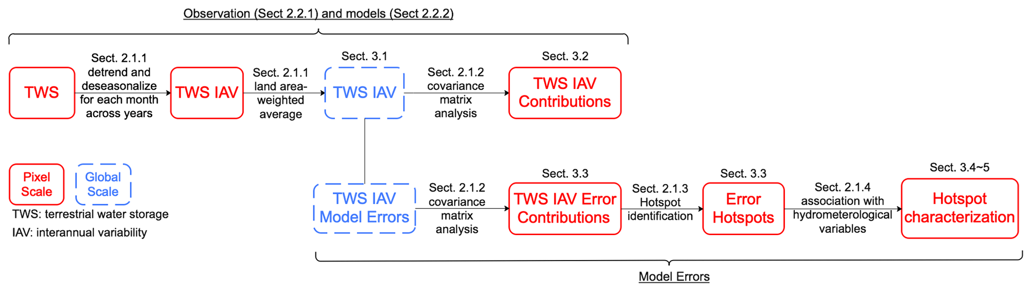
Figure 1Schematic overview of the methodology to diagnose modeling errors in the simulation of the global TWS IAV. The sections of the paper that cover different aspects of the analysis are provided with section headings.
2.1 Methods
2.1.1 Calculation of interannual variability
In this study, the IAV metric quantifies how much a certain data value (e.g., TWS) deviates from the long-term (i.e., trend) and mean seasonal variation. Accordingly, we calculated TWS IAV of each pixel as follows:
where X is a time series of TWS anomalies after removing the pixel mean, i is a pixel, m is a month of the year, and fit( ) is the fitted values of a linear regression model over a time series of a month across years. In other words, the linear trend is fitted across all years for each month (see Fig. B1 for an illustration). The mean for the study period (April 2002–June 2017) was removed from the GRACE TWS anomalies or model TWS estimates for each pixel. This was done (1) to convert model TWS estimates to TWS anomaly estimates and (2) to align different TWS anomaly products with the same baseline period.
Using the TWS IAV of each pixel, we calculated the globally integrated GRACE TWS IAV scaled by the area of each pixel as follows:
where IAVglobal,m is the global IAV for each month (m), which is calculated for both observation () and model simulations (), i is a pixel, and Ai is the area of pixel i. We multiplied TWS by the pixel area so that the resulting TWS IAV is independent of the area of the pixel which is dependent on the map projection. Then, the modeled error is calculated as a residual of global TWS from observations and models as follows:
where “err” indicates errors. A positive error therefore stands for an overestimation by a model.
2.1.2 Spatial attribution of the globally integrated signal
The variance in globally integrated TWS IAV and its error was attributed to each land pixel using a covariance matrix method. A covariance matrix calculated using the time series of land pixels contains the covariance of TWS IAV between a pair of pixels as the off-diagonal elements (for each combination of two different pixels) and the variance in TWS IAV in each pixel as the diagonal elements. By calculating the row (or column) sum of the covariance matrix scaled by the total sum, the contribution of a pixel to the variance in the globally integrated value can be quantified as follows:
where fi is the relative contribution of pixel i, Xi is a random variable (i.e., TWS IAV or TWS IAV error) of the pixel i, Var(Xi) is the variance for pixel i, and Cov(Xi,Xj) is the off-diagonal element at the ith row and jth column in a n×n covariance matrix, where n is the number of land pixels in the globe. On the right-hand side of the equation, the numerator is the sum of the elements of the ith row (or column); the denominator is the sum of all the elements of the covariance matrix. This method quantifies the contribution of each pixel in a relative and normalized term; by definition, the sum of the contributions of all pixels becomes one. It also considers the sign of the contribution. A large positive covariance for a pixel means that the pixel increases the global variance, implying that the pixel has a similar temporal pattern to the global one. In contrast, a large negative covariance means that the pixel compensates with the global variability. The calculated fi is mathematically additive.
2.1.3 Hotspot identification
We calculated the R2 between the globally integrated time series of GRACE and the models (Sect. 2.1.1) to evaluate the model performance of TWS. The R2 values were iteratively calculated after trimming out pixels that have large positive contributions to the variance in global TWS IAV errors (fi in Eq. 4). The large positive covariances were trimmed because the purpose of this study is to identify pixels that contributed to the emerging global variability in TWS errors; in this method, pixels with positive contributions shape the global signal, while pixels with negative contributions partly compensate for the signal. For the trimming percentile, 0.0 % (i.e., no trimming), 0.1 %, 0.3 %, 0.5 %, 1 %, 2 %, 3 %, 5 %, and 7 % and from 10 % to 50 % with 5% intervals were used. An increase in R2 after trimming suggests that the pixels of large positive contributions negatively affect the model performance in simulating the TWS IAV. In other words, correcting simulations in those pixels can improve the model performance at the global scale.
2.1.4 Association with hydrometeorological variables
After the error hotspots are identified, we compare the time series of TWS and precipitation IAVs at the regional scale for error hotspots within selected Intergovernmental Panel on Climate Change (IPCC) Special Report on Managing the Risks of Extreme Events and Disasters to Advance Climate Change Adaptation (SREX) regions (Sect. 3.4; see Fig. B2 for the SREX regions) to diagnose TWS IAV errors. This association is simply quantified using the correlation coefficient between TWS and precipitation IAVs. Note that the SREX regional classification has been extensively used to diagnose the regional variation in the global climate model simulations (e.g., Seneviratne et al., 2012; Pokhrel et al., 2021).
In addition, we associate the error with selected hydrological variables, and we test if the variable can characterize hotspots from non-hotspots. As both the models were forced by the climate variables, we assume that the model errors are less likely to be associated with climate characteristics and select variables that are related to missing model processes (see Sect. 2.2.3).
The association between the hotspots and the selected variables is inferred by comparing the histograms of hydrometeorological variables in hotspot and non-hotspot (see Sect. 2.1.3 for the hotspot identification) regions. The histograms, for hotspots and non-hotspots, of the different variables were computed across equal-sized bins. We additionally provide the probability density curve that was estimated using the Gaussian kernel whose bandwidth was determined with Scott's (https://doi.org/10.1002/9780470316849) rule of thumb. We then calculated the difference in the bin heights of the two histograms (hotspots minus non-hotspots) to find if the variable characterizes hotspots from non-hotspots. Positive (negative) differences mean that error hotspots have a higher (lower) probability density than non-hotspots for the given values of a selected variable. Based on the differences, we assume that a variable which shows a clear positive difference in the histograms of hotspots and non-hotspots are influential in and potentially the source of error in the models.
2.2 Data
In this section, we introduce the data sets used in the analysis. First, we introduce the GRACE TWS observation data. This is followed by brief descriptions of two hydrological model simulations used to compare against GRACE. Last, we summarize the ancillary hydrometeorological data used for characterizing error hotspots.
2.2.1 GRACE TWS observation
For the TWS observation, we used a release 6 (RL06) mass conservation (mascon) solution Level-3 monthly TWS anomaly product provided by the Jet Propulsion Laboratory (JPL; Wiese et al., 2016). The mascon solution is known to have lower leakage errors compared to the traditional spherical harmonic solution (Scanlon et al., 2016). The product is provided at spatial resolution, even though the native observational resolution of GRACE satellites is 3∘ (Wiese et al., 2016). The data are available for the period of April 2002 to June 2017. GRACE provides a vertically integrated estimate of TWS variations as anomalies relative to the observations from January 2004 to December 2009. A glacial isostatic adjustment has been applied using the ICE6G-D model from Peltier et al. (2018) to exclude signals due to solid-Earth deformation. The coastline resolution improvement filter and a set of scaling factors were applied to reduce leakage errors between land and ocean (Wiese et al., 2016). Nevertheless, GRACE TWS still contains errors from measurement and leakage. Generally, GRACE errors (1) increase with decreasing latitudes toward the Equator due to the polar orbit of the twin satellites (Frappart and Ramillien, 2018) and (2) are large at land–ocean boundaries due to the signal leakage (Wiese et al., 2016). The scaling factors are also incomplete in ice-covered regions and near inland waterbodies, where the land-surface-model-derived scaling factors are less reliable (Wiese et al., 2016).
2.2.2 Global hydrological model simulations
We analyzed simulations of TWS variations from two data-driven global hydrological modeling approaches, including (a) a conceptual hydrological process-based model configured using a model–data integration framework, strategies to integrate data and biogeochemical models (SINDBAD), and (b) the hybrid hydrological model (H2M), using a hybrid approach that fuses hydrological balance equations with a dynamic neural network. Both models were calibrated to hydrological data streams, including TWS observations from GRACE. This makes the model errors less likely to be caused by parameter values, allowing us to focus more on the model structure and represented processes, while analyzing errors. Owing to the use of observational data, SINDBAD shows a similar or better performance in simulating TWS seasonality and IAV compared to an ensemble of global hydrological and land surface models (Trautmann et al., 2018). H2M has also been applied for different climatic regions over the globe to simulate TWS seasonality and interannual variability, where it is shown that H2M is capable of learning key patterns of the global water cycle components and has a comparable performance and better local adaptivity, compared to four state-of-the-art global hydrological models (Kraft et al., 2022). In summary, the two model simulations used here provide state-of-the-art hydrological models, where the model parameters and processes are partly learned from GRACE observations and are comparable to the state-of-the-art hydrological models commonly used.
SINDBAD, constrained with multiple observational data streams, has been successfully applied over northern mid-to-high latitudes (e.g., Trautmann et al., 2018) and over the globe (Trautmann et al., 2022) to simulate the seasonality and interannual variability in TWS and its components. SINDBAD is a simple, conceptual, four-pool water balance model with spatial variations in hydrological parameters, depending on remote sensing and statistical estimates of vegetation fraction and soil water capacity (Trautmann et al., 2022). SINDBAD TWS consists of snow, soil moisture divided into shallow and deep components, and delayed moisture storage. Model parameters were constrained using TWS, snow water equivalent, evapotranspiration (ET), and runoff observations, as well as vegetation characteristics including vegetative activity and maximum rooting depth.
The hybrid hydrological model (H2M; Kraft et al., 2020, 2022), on the other hand, uses a hybrid approach that fuses the hydrological balance equations and a neural network and provides an even stronger data-driven estimate of TWS variations. In H2M, the hydrological balance equations define three types of storage, namely snow water equivalent, soil water deficit (storage is represented as the additive inverse/opposite of the deficit), and groundwater. The model is driven by data of the time-varying meteorological forcing and time-static soil and land characteristics. Five parameters (soil recharge fraction, groundwater recharge fraction, fast runoff fraction, snowmelt coefficient, and evaporative fraction) are estimated by a dynamic neural network and used as the time-varying parameters in the balance equations. The first three parameters partition the incoming moisture fluxes, and the last two quantify snowmelt and evapotranspiration, respectively. The dynamic neural network updates each parameter value as a function of the storage status of the previous time step, meteorological forcings of the present time step, and static variables for each pixel globally, resulting in spatiotemporally varying hydrological parameters that enable a large data adaptability of the hybrid approach. Observational constraints of TWS, snow water equivalent, evapotranspiration, and runoff were used for model tuning, and some static variables such as elevation, soil property, and land cover type were used as additional model inputs.
While both modeling frameworks are predominantly data-driven, there are some key differences between them. First, H2M is more flexible and adaptive to the data used, as H2M deploys the dynamic neural network to partition fluxes. Second, two models use additional data sets for the parameter estimation in addition to hydrological pools and fluxes that are used as constraints. SINDBAD uses vegetation-related input such as the vegetation greenness index and rooting depth, although the vegetation variables do not vary spatially and interannually. H2M additionally uses some static variables related to soil properties, topography, and land cover. Last, the structure of the water pools is different. SINDBAD has two soil layers, namely an upper one with a fixed moisture capacity (4 mm) and a deeper one with a moisture capacity estimated from different data sets during the calibration process. H2M, on the other hand, approximates soil moisture as a cumulative deficit via a data-driven approach that does not require a prescription of the soil moisture storage capacity. Moreover, H2M implicitly learns the layering of soil moisture to a certain extent (Kraft et al., 2022). In SINDBAD, the transpiration supply has access to the deeper soil moisture layer. H2M implicitly represents it as a function of soil water deficit. SINDBAD represents groundwater storage via deep and delayed storage, which are interacting through the drainage flux and capillary rise, while H2M directly represents a single groundwater storage that is fed by a drainage flux without a capillary rise. The delayed moisture storage of SINDBAD implicitly represents all water storage components that may delay the loss of moisture from the system, and that includes surface water variations as well, while H2M does not account for surface water storage. In both models, part of the excess throughfall forms fast direct runoff, while baseflow (or slow runoff) is generated from delayed moisture storage in SINDBAD but groundwater in H2M. Finally, the TWS is a sum of snow, soil, and deep and delayed storage for SINDBAD and snow, soil, and groundwater for H2M.
For consistency, a common set of forcings and constraints were used to force the models and calibrate the model parameters at spatial and daily temporal resolutions (see Appendix A).
2.2.3 Ancillary data
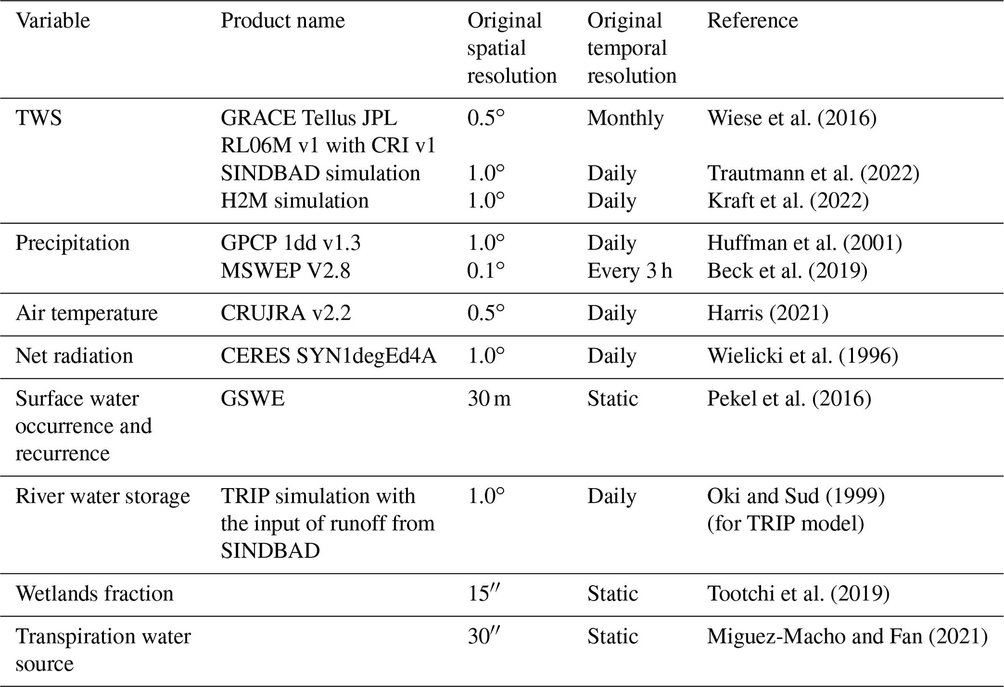
The ancillary data were used to explore the potential association of the modeled TWS errors with hydrometeorological variables (Table 1). All variables were aggregated into the 1∘ spatial and monthly temporal (for temporally varying variables) resolutions using the land area of each pixel. In this section, we briefly summarize the data set used.
Wiese et al. (2016)Trautmann et al. (2022)Kraft et al. (2022)Huffman et al. (2001)Beck et al. (2019)Harris (2021)Wielicki et al. (1996)Pekel et al. (2016)Oki and Sud (1999)Tootchi et al. (2019)Miguez-Macho and Fan (2021)Table 1Data used to associate with modeled terrestrial water storage (TWS) errors.
2.2.4 Climate variables
As the main drivers of TWS variability over land, we compared the IAV (i.e., Eq. 1) of the three forcing variables (precipitation, air temperature, and net radiation) with TWS IAV (Sect. 3.4). We also calculated the standard deviation of IAV of the forcing variables of each pixel and compared the distribution of the standard deviation between error hotspots and non-hotspots to characterize the error hotspots. An additional observation-based precipitation product was used to check if the patterns vary across different precipitation products. For that, we used the Multi-Source Weighted-Ensemble Precipitation, version 2.8 (MSWEP V2.8; Beck et al., 2019), product that merges rain gauge, satellite, and reanalysis precipitation estimates.
2.2.5 River water storage
The river water storage wRiver is considered to be a proxy for the surface water quantity. We assume that the regions with a large wRiver have a significant contribution of the surface water component to the total TWS. For this analysis, wRiver was calculated using the Total Runoff Integrating Pathways (TRIP) river routing model (Oki and Sud, 1999), with the input of runoff from SINDBAD model simulations. Daily wRiver was averaged to monthly values, and then monthly wRiver was converted to the absolute storage by multiplying the area of each pixel. The volumetric unit was used because the absolute storage, not the equivalent height, was used to calculate the model biases (see Sect. 2.1.1). The maximum wRiver of a pixel (wRivermax) during the study period (April 2002–June 2017) was used for comparing its probability density distribution between error hotspots and non-hotspots. We applied log transformation to wRivermax before comparing the probability density distribution to alleviate its skewed distribution.
2.2.6 Wetlands fraction
To distinguish different surface water dynamics that are either associated with permanent river waterbodies or seasonally dynamic storage interactions, we consider the wetland fractions data set from Tootchi et al. (2019). The data set contains seven composite maps that include wetlands of two classes, namely (1) regularly flooded wetlands created from three satellite-derived data sets of open water and inundation and (2) groundwater-driven wetlands from water table depth estimations of Fan et al. (2013) and three topographic indices with two thresholds. Among the seven composite maps, Tootchi et al. (2019) provide two composite maps that showed the best similarity scores to the reference data sets. The two composite maps have many similarities, such as the spatial distribution and extent of wetlands (Tootchi et al., 2019), and the one using the topographic index (CW-TCI15) was used in this study. The data set was averaged into 1∘ spatial resolution. The probability density distribution of each class of wetlands, excluding their intersection, was compared between error hotspots and non-hotspots. Regularly flooded wetlands represent the river storage dynamics, while groundwater-driven wetlands indicate the propensity for interactions among soil water, groundwater, and surface water due to the shallow water table depth.
2.2.7 Groundwater usage by vegetation
We evaluate the relevance of different moisture sources in the evaporative process, which in turn affects the TWS dynamics, by evaluating the associations of moisture sources for transpiration with occurrences of hotspots. In order to do so, we used the transpiration source partitioning data set by Miguez-Macho and Fan (2021). The data set considers four sources of transpiration, such as (1) precipitation in the current month, (2) past precipitation stored in unsaturated soils, (3) locally recharged groundwater via capillary flow, and (4) remotely recharged groundwater from uplands to lowlands. Note that the remotely recharged groundwater indicates the groundwater converged topographically (Miguez-Macho and Fan, 2021), which was originally estimated at a high spatial resolution of 30 arcsec. Using the map of the annual mean contribution aggregated to 1∘ (one was used for Fig. 2 in Miguez-Macho and Fan, 2021), we compared the probability density of the contributions of capillary flow and converged groundwater from uplands between error hotspots and non-hotspots.
2.2.8 Surface water existence
To investigate the relationship between TWS IAV error and the propensity of the existence of surface water, we used Landsat-based data for surface water existence from the Global Surface Water Explorer (GSWE; Pekel et al., 2016). Among the set of GSWE variables, we used two static variables, i.e., occurrence and recurrence. Briefly, the occurrence is calculated with the following steps: (1) calculate the ratio of the number of valid observations with surface water detected to the total number of valid observations for each month of the year (i.e., 12 values in total) and (2) average the 12 values. This two-step calculation normalizes the occurrence against the seasonal variation in the number of observations, otherwise the occurrence is biased by the temporal variation in the valid observations of the pixel (Pekel et al., 2016). Recurrence is calculated as the number of years with at least one valid observation with surface water detected divided by the number of years with at least one valid image collected. The occurrence thereby provides a general overview of the frequency of surface water existence, while recurrence represents the interannual fraction of the surface water.
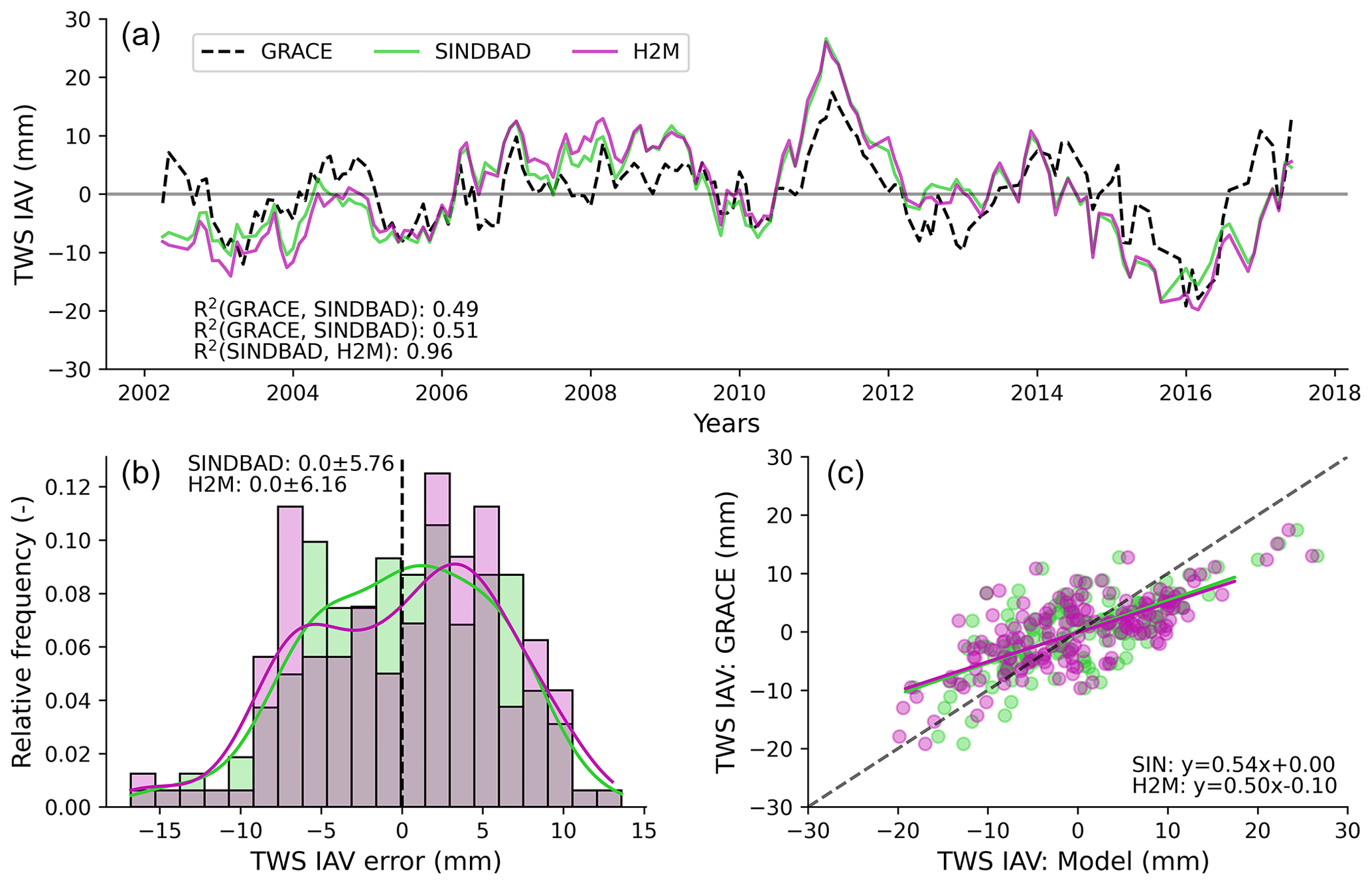
Figure 2Comparison of monthly global terrestrial water storage (TWS) interannual variability (IAV) from GRACE observations and two data-driven hydrological models (SINDBAD and H2M). (a) Time series comparison of monthly global TWS IAV. R2 statistics in the bottom left are calculated as the square of the Pearson correlation coefficient. (b) Histogram of errors in the global TWS IAV (Eq. 3), with smoothed kernel density curves estimated using the Gaussian kernel and Scott's rule of thumb to determine the bandwidth of the kernel. The sum of all bar heights (different models in different colors) equals unity. The text shown in the upper left is the mean ± standard deviation of the distribution of each model. (c) Scatterplot of monthly TWS IAV by GRACE and models. Equations in the bottom right are from a robust linear regression using Huber's (https://doi.org/10.1002/0471725250) T estimation for down-weighting outliers.
For occurrence, to calculate the spatial fraction of surface water domination, we first assigned a value of 1 for the raster of 30 arcsec when the occurrence value is larger than a threshold value (50 %) and 0 otherwise. We then spatially averaged the raster of 30 arcsec to 1∘ spatial resolution using valid observations only. For recurrence, we spatially averaged the raster of 30 arcsec to 1∘ spatial resolution, as the data are already suitable for representing temporal fraction of surface water presence. A coastline mask (Sayre et al., 2019) was applied to occurrence and recurrence data sets before the aggregation to exclude possible biases of high occurrence and recurrence in coastal regions. We used the derived occurrence as a proxy for spatial existence. For the temporal existence of surface water, we used a product of occurrence and recurrence (i.e., recurrence multiplied by 1 occurrence). The product accounts for the interaction between occurrence and recurrence and excludes pixels dominated by permanent existence or a complete lack of surface waterbodies (i.e., either recurrence or 1 occurrence becomes 0). This assigns larger values to the regions where the presence of surface water is temporally erratic (high recurrence and low occurrence) but significant, which may lead to a large IAV of TWS.
In this section, we first compare modeled and GRACE global TWS IAV to obtain a glimpse of the model performance and errors (Sect. 3.1). We continue to introduce pixel-wise contributions to the variance in global TWS IAV in GRACE and models (Sect. 3.2) and model errors (Sect. 3.3), followed by an inspection of the time series of TWS IAV and precipitation IAV for selected regions (Sect. 3.4). We finally investigated the association of the global TWS IAV errors to hydrological variables, including surface water dynamics and groundwater usage by vegetation (Sect. 3.5).
3.1 Global TWS interannual variations
SINDBAD and H2M reasonably reproduce the observed time series of global TWS IAV by GRACE (R2 of 0.49 and 0.51 for SINDBAD and H2M, respectively; Fig. 2) in addition to the spatial patterns of TWS anomaly and TWS IAV (Figs. B3 and B4). The modeled and observed variations are generally similar in the sign of the variations (positive or negative anomalies). Interestingly, the two models show similar temporal variations (Fig. 2a) with R2 of 0.96, despite differences in the modeling perspectives (i.e., process based with calibrations against observations vs. machine-learning-based estimates with only mass balance principles). Regarding the distribution of errors, the differences between estimates and observations are mostly <10 mm and normally distributed with a mean of 0, suggesting that models generally perform well (Fig. 2b).
Despite the overall good performance, the models overestimate the observed magnitude of GRACE in both tails. For instance, the models overestimated the magnitude of globally wet conditions in 2011 and dry conditions in 2015–2016 (Fig. 2a). This pattern of the overestimation of magnitude is also prevalent in non-extreme years, such as 2002 and 2006 to 2009, which results in the lower R2. The scatterplot between estimates and observations shows a cluster in a TWS IAV from −10 to 10 mm (Fig. 2c). The cluster is positioned around the one-to-one line but is rather less constrained, resulting in regression slopes of 0.54 for SINDBAD and 0.50 for H2M. These slopes mean that the models overestimate (i.e., more positive) wet conditions, while they underestimate (i.e., more negative) dry conditions. The overestimation is probably due to the fact that the models lack interactions between water storage that reduce TWS IAV. For example, surplus runoff can be redistributed within and across pixels via lateral flow to replenish rather dry regions, which is not simulated by the models.
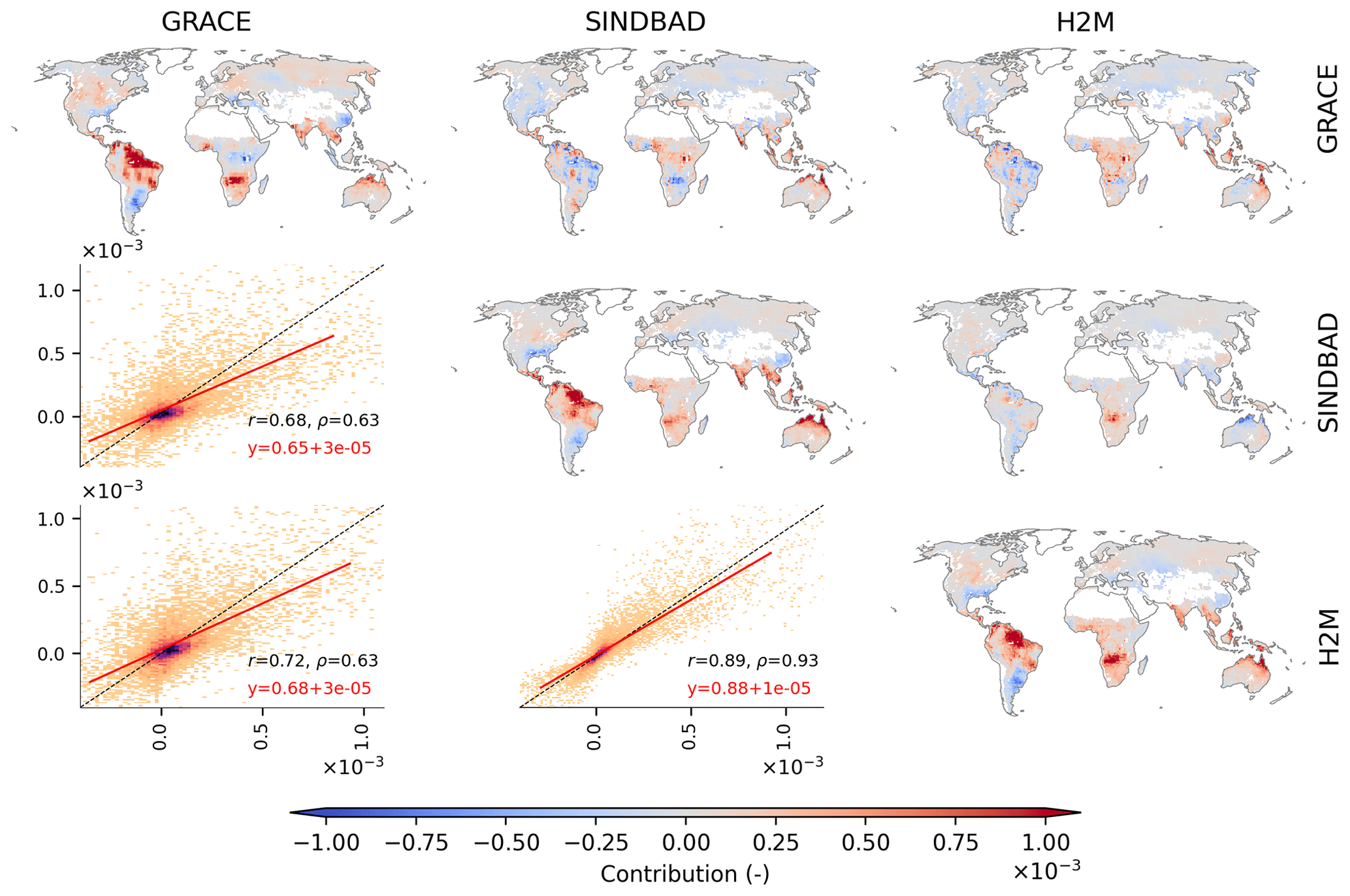
Figure 3Global distribution of pixel-wise contributions to the variance in the global terrestrial water storage (TWS) IAV. Along the diagonal, maps of the pixel-wise contribution in GRACE, SINDBAD, and H2M are shown (indicated by the label of the row or column). Above the diagonal, maps of the difference (i.e., column−row) are shown. For example, the map of the first row and the second column is for SINDBAD (column) minus GRACE (row). Below the diagonal, scatterplots comparing the pixel-wise contributions of the corresponding column (x axis) versus row (y axis) are shown. In the scatterplots, colors indicate the density of point, r is the Pearson correlation coefficient, and ρ is the Spearman correlation coefficient. Red lines are the linear regression fit, and red text refers to the corresponding equations. White pixels within land boundaries are the regions masked out in this study (see Appendix A).
3.2 Spatial contributions to the global TWS IAV
While the models perform generally well in terms of reproducing the global TWS IAV, the differences in amplitude are significant. We conduct a covariance matrix analysis to quantify the spatial contributions of each pixel to the variance in the global TWS IAV.
The modeled TWS IAV generally agrees with the pattern from GRACE (maps along the diagonal in Fig. 3), with correlation coefficients of 0.68 and 0.73 for SINDBAD and H2M, respectively. The spatial patterns are also consistent among two models (r=0.89). GRACE and the models agree that the strongest positive contributions appear in the humid regions of northern South America and the Mekong River basin in addition to the semi-arid regions of southern Africa, the Indian subcontinent, and northern Australia (Fig. 3). On the contrary, strong negative contributions are from southeastern South America, central Africa, and southeastern China.
Despite the broad similarity, there are some differences between GRACE and the models. For instance, the negative contribution of sub-Saharan regions in GRACE is not prominent in the models, and positive contributions in humid regions of Southeast Asia and northern Australia are stronger in the models (maps above the diagonal in Fig. 3). The models tend to underestimate the lowermost contributions and overestimate the largest contribution, which results in a slope < 0.68 and intercept > 0 for the fitted lines (Fig. 3). There are also subtle differences between SINDBAD and H2M, with H2M showing a larger contribution from the Okavango region and a smaller contribution from northern Australia, which results in a slightly better comparison between GRACE and H2M. In summary, GRACE and both models show a globally spread out pattern of contributions to the global TWS IAV. The difference in patterns between GRACE and the models is not coherent with climate alone, as the differences are clear in both humid and semi-arid regions.
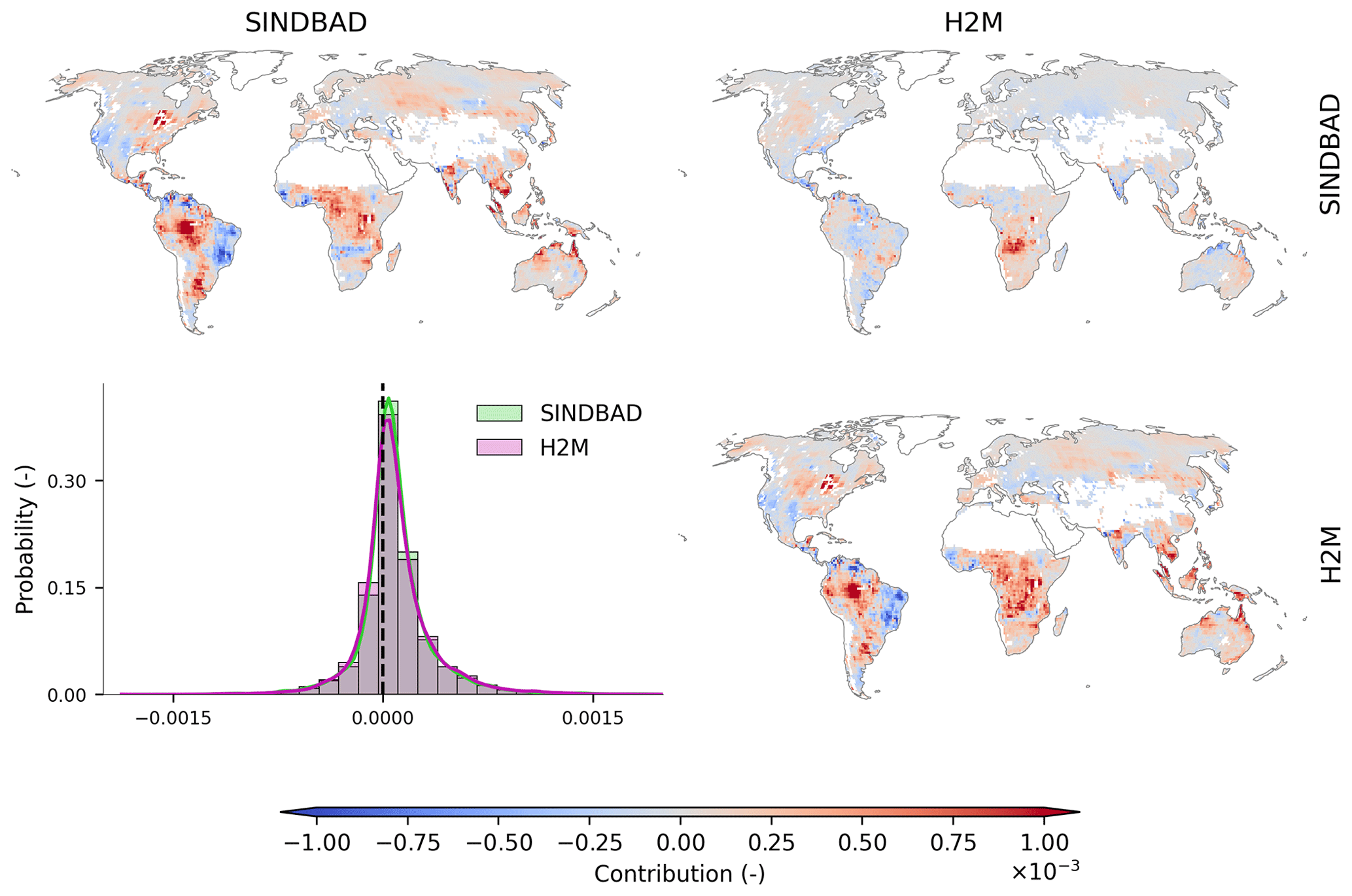
Figure 4Global distribution of pixel-wise contributions to the variance in the modeling error in the global terrestrial water storage interannual variability. Along the diagonal, maps of the pixel-wise contribution to the global TWS IAV modeling errors in SINDBAD and H2M are shown. Above the diagonal, a map of the difference (i.e., H2M−SINDBAD) is shown. Below the diagonal, a histogram comparing the corresponding column (x axis) versus row (y axis) is shown. The probability density curves were estimated using the Gaussian kernel and Scott's rule of thumb to determine the bandwidth of the kernel. White pixels within land boundaries are the regions masked out in this study (see Appendix A).
3.3 Spatial contributions to the global TWS IAV error
We showed that the patterns of the contributions of each pixel to the global TWS IAV are largely consistent among the models and GRACE, but the question remains as to whether these regions also contribute to the error in global TWS IAV. We, therefore, apply the same covariance matrix analysis to the globally integrated TWS IAV errors (Eq. 3) to identify the regions which contribute to the variance in the error and identify the global error hotspots.
Despite the differences in the model processes and how data were used, the two models generally agree on the distribution of the error contributions (Fig. 4). The strongest positive contributions to the variance in the error appear in the Laurentian Great Lakes basin, the Amazon, the Paraná River lowlands, sub-Saharan regions, the Indian subcontinent (Narmada, Tapi, and Godavari river basins), Southeast Asia, and northern Australia. For H2M, areas of positive contributions mostly coincide with areas showing strong errors in the TWS IAV simulation reported by Kraft et al. (2022). Negative contributions appear in the semi-arid regions of northeastern South America, western North America, and Eastern Europe. The contribution of a pixel is barely related to the relative uncertainty in GRACE observations (Fig. B5), implying other causes of the modeling error. The distribution of contributions is centered around 0 but with a longer positive tail (histogram of Fig. 4). This suggests that a few pixels have a relatively larger positive contribution to the variance in the global TWS IAV errors. We, therefore, identify these influential pixels (hereafter the error hotspots) which have the largest influence on the change in (1) the contributions to the variance in global TWS IAV errors and (2) R2 between the models and GRACE.
When the hotspot pixels are trimmed, we indeed find that the model performance improves and the error contribution to the variance in the global TWS IAV error reduces (Fig. 5). For example, the pixels with the largest 10 % error contribution explain 70 % of the variance in the global TWS IAV error. At the same 10 % trimming, R2 for global TWS IAV improves from 0.49 to 0.70 for SINDBAD and from 0.51 to 0.77 for H2M. Note that the model improvement seizes or reverses when larger percentiles are trimmed because of the loss of variance signal in the data. The results, though, confirm that a small portion of pixels (10 %) is highly influential for modeling simulation errors at the global scale, and thereby, those pixels can be regarded as hotspots of the global TWS IAV errors. In fact, models perform much worse in error hotspots (R2 ranges from 0.00 to 0.52 across model–region combinations; Fig. 6) than they perform at the global scale (Fig. 2); models show much better performances in non-hotspots (R2 ranges from 0.54 to 0.95 across model-region combinations; Fig. B6) than they do in error hotspots. On a broad scale, the error hotspots, mostly in tropical regions (Fig. B7), are common between the two models, suggesting common, potentially missing, mechanisms. At the regional scale, the error hotspots of each model (and their intersection) may differ slightly.
Note that the hotspot regions for error are not necessarily fully consistent with regions with the largest contribution to the global TWS IAV, as the contributions have a low spatial correlation (Fig. B8). While the global TWS IAV signal is mainly dominated by moisture-limited semi-arid regions (Fig. 3), most of the error hotspots are identified in tropical regions, which means that the regions with large contributions to the variance in global TWS IAV are not necessarily the same as those that contribute to the error in the variance in global TWS IAV (Fig. B8). In addition, the error hotspots are located over large river networks, wetlands, or around lakes, which suggests the possible role of surface water dynamics in TWS variability.
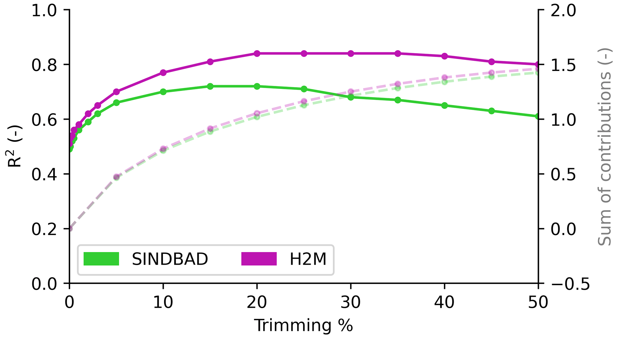
Figure 5Changes in model performance and errors when pixels with the largest contribution to the variance in global TWS IAV errors are trimmed. Solid lines show changes in R2; dashed lines show the sum of the contributions of the corresponding trimmed-out pixels.
3.4 Temporal variation in TWS and climate in error hotspots
To characterize the hotspot regions and evaluate if TWS errors are systematic across time, we present the temporal variation in TWS IAV and precipitation IAV at the regional scale for different error hotspots within selected SREX regions (see Fig. B2 for the SREX regions). Note that the temporal variations in other climatic variables for the same regions are shown in the Appendix (Figs. B9 and B10).
Across the error hotspots of all selected SREX regions, modeled TWS IAV shows stronger correlations with precipitation than GRACE, suggesting that the processes, such as lagged storage variations that are not directly related to annual precipitation, play a key role in TWS IAV. The pattern is consistent even when an independent precipitation product is used (Fig. B11). In addition, while models overestimate the range (or amplitude) of global TWS IAV (Fig. 2), the regional-scale errors are bidirectional. For example, in the Laurentian Great Lakes (Fig. 6a), both positive and negative peaks (e.g., 2005–2006 and 2010–2014) are underestimated by the models. Moreover, in the Amazon (Fig. 6b), the peaks of TWS in drought (2010) and floods (e.g., 2009) (Chen et al., 2010) are not well captured.
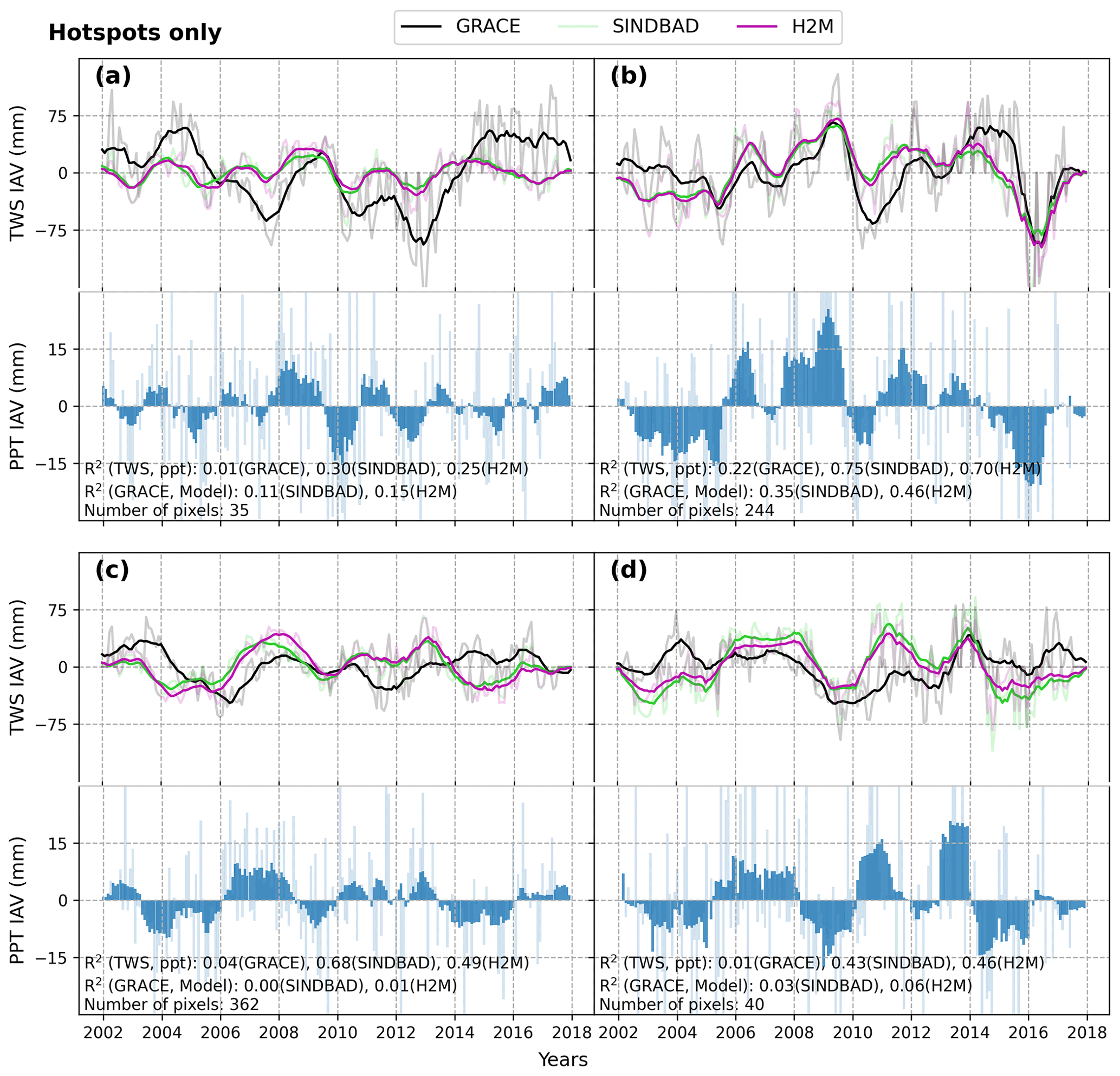
Figure 6Time series of 12-month moving averages of GRACE and modeled terrestrial water storage (TWS) interannual variability (IAV) in error hotspots that are commonly identified by SINDBAD and H2M (Fig. B7) within each selected region. The Laurentian Great Lakes (a; region 5), the Amazon (b; region 7), eastern and western Africa (c; regions 15 and 16), and South Asia (d; region 23) are shown. SREX regions are shown in Fig. B2. Monthly values are shown with faded colors.
3.5 Association with hydrological variables
While we have identified the hotspots of global TWS IAV errors, the potential reasons and sources of the errors in these regions are yet not clear. To further understand how the models, which were actually forced by climate variables, could not simulate the TWS IAV well in these regions, we contrast the distribution of hydrological variables in error hotspots and non-hotspots to infer the possible hydrological mechanisms behind the errors. As the model simulations were forced with climate, and parameters were constrained with the evapotranspiration and runoff data (see Appendix A), we focus on the variables that are reflective of the missing processes in the selected models. In particular, we focus on the missing processes of surface water dynamics and local- and regional-scale lateral moisture convergence, which may result in biases in runoff and ET processes and consequently affect the TWS variability. Note that the association with the climate variables, which form the necessary predicate for TWS variability in the model simulations, are presented in Fig. B12.
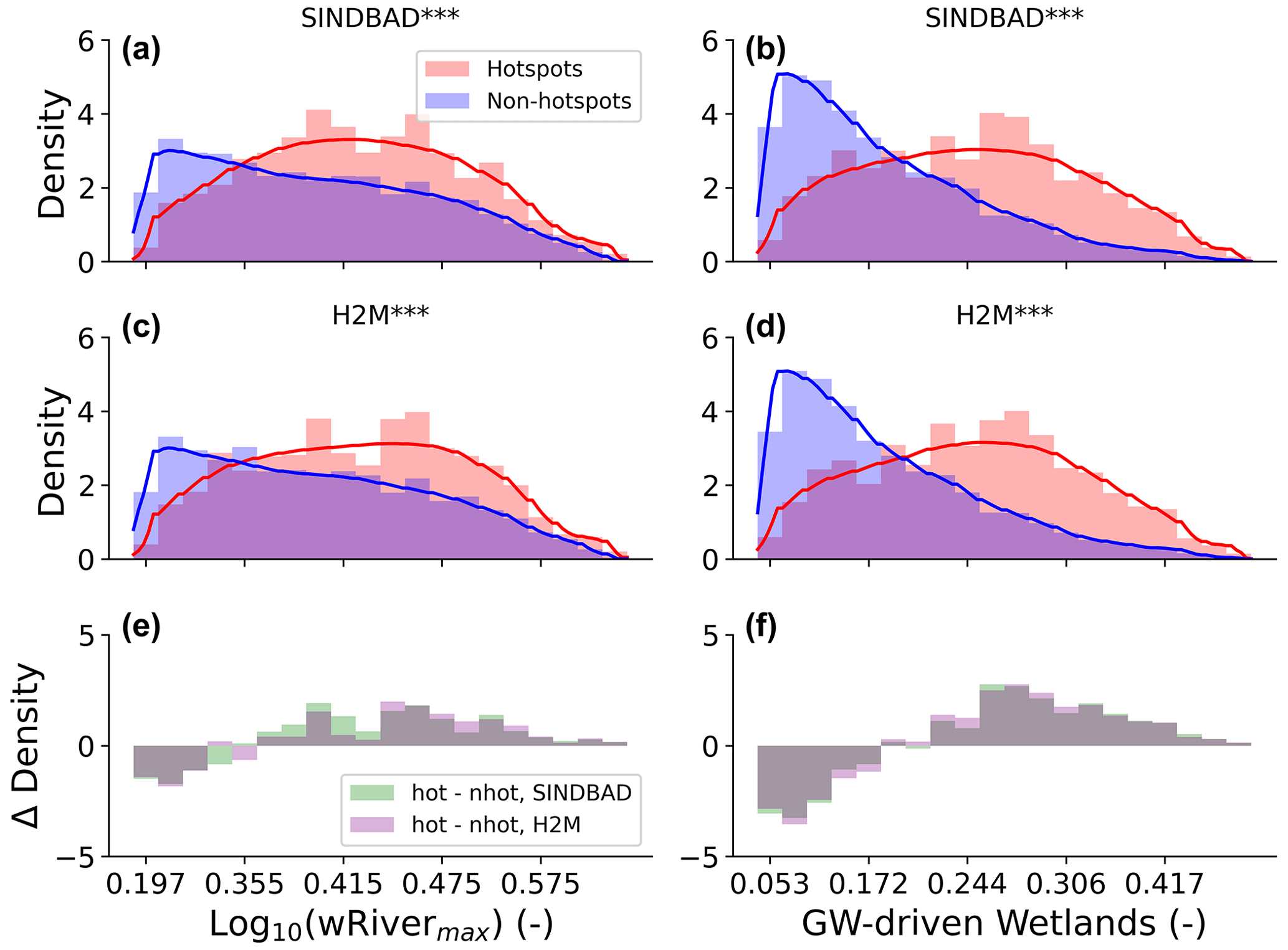
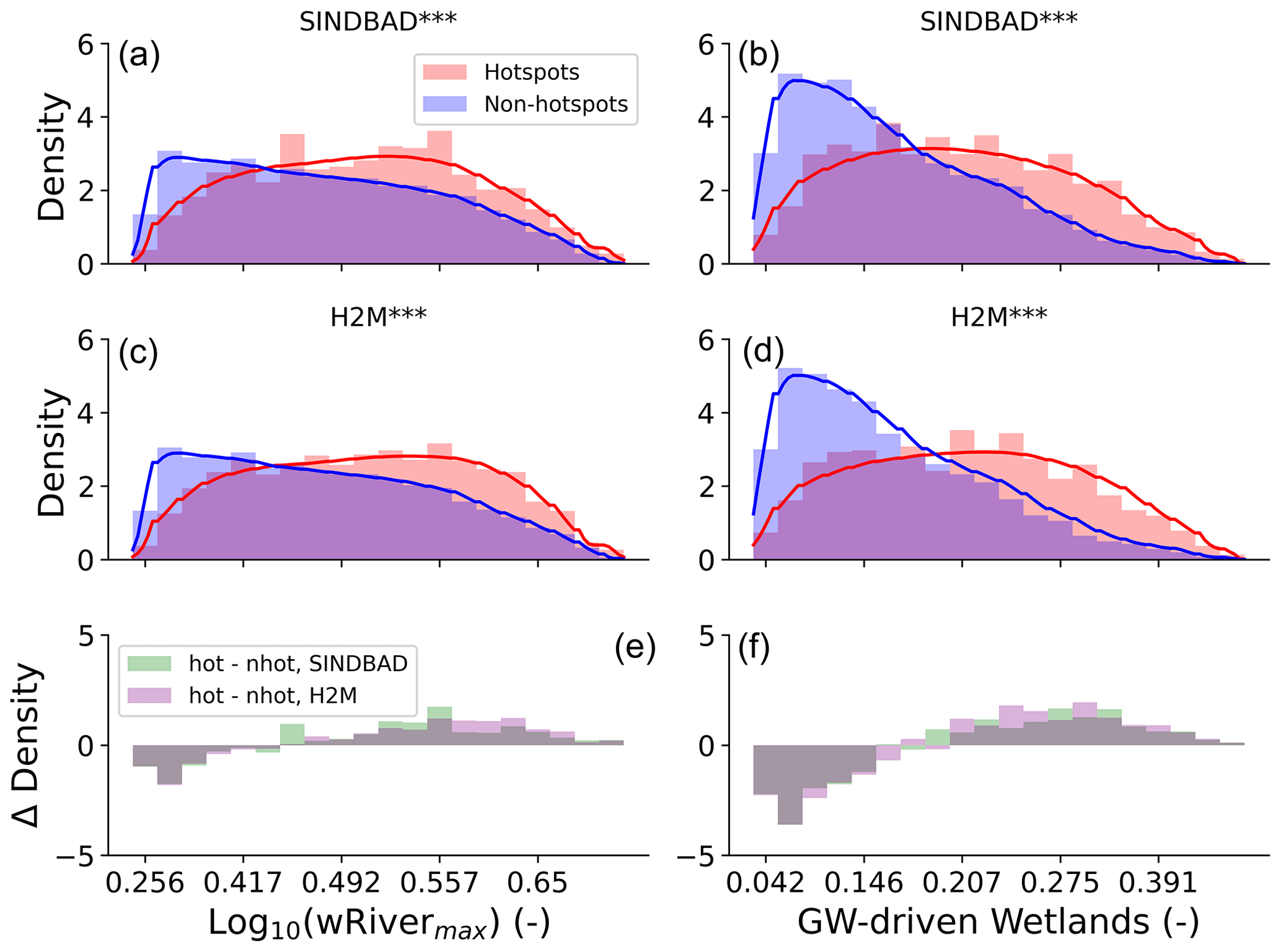
Figure 7Comparison of probability density distributions of the log-transformed maximum river water storage (a, c, e) and wetland fraction (b, d, f) between the error hotspot pixels and non-hotspot pixels. Panels (a)–(d) are the distributions of each model; panels (e) and (f) show the difference in the bar heights between the hotspots and non-hotspots (positive means occurrences are larger in error hotspots). The probability density curves were estimated using the Gaussian kernel and Scott's rule of thumb to determine the bandwidth of the kernel. Asterisks (*) beside the model names show the significance of the difference in the distributions between the error hotspots and non-hotspots using the Kolmogorov–Smirnov two-sample test; all results show the significant difference in the distributions (; p value < 0.001). Note that the x axis is normalized using the maximum and minimum of variables so that the range becomes 0 to 1 and comparisons can be made across variables. The river water storage (wRivermax) was calculated using the Total Runoff Integrating Pathways (TRIP) river routing model (Oki and Sud, 1999) with the input of runoff from SINDBAD. The maximum wRiver of a pixel (wRivermax) during the entire period (April 2002–June 2017) was used with log transformation to use the skewed distribution of (wRivermax) for comparison. The fraction of groundwater-driven (GW-driven) wetlands was provided by Tootchi et al. (2019).
The error hotspots show a systematic larger probability density of larger maximum river storage (Fig. 7), which indicates the possible relevance and significance of river storage for the TWS interannual variability in the error hotspots. The two selected models do not explicitly account for the river or floodplain storage that accumulates large amounts of lateral flow of flood water. This means that the model would not account for the runoff loss that is included in the delayed TWS variation, as one would expect in large river basins. Furthermore, error hotspots show larger fractions of groundwater-driven wetlands (Fig. 7), while they show smaller fractions of regularly flooded wetlands (Fig. B13), suggesting a role of surface water–groundwater dynamics as well. The dominance of groundwater-driven wetlands in error hotspots indicates that the water table depth in error hotspots is rather shallow, which forms the necessary conditions for a strong interaction among soil water, groundwater, and surface water. On the other hand, the spatial and temporal fractions of the surface water existence do not characterize error hotspots from non-hotspots (Fig. B14). This rather unclear difference in surface water existence compared to river water storage may be related to (1) very local occurrences (compared to large global area) of surface water and/or (2) a lack of quantitative measurements of water storage in the patterns of surface water existence. For example, the surface water may exist in most years in both the hotspots and non-hotspots, whereas the magnitude of existence (e.g., the number of months) can still be different, but this cannot be distinguished from the given data.
The error hotspots are also common in monsoon regions, where a clear seasonal variation in precipitation amplifies the role of secondary moisture sources on evapotranspiration processes (Koirala et al., 2014) that consequently determine the TWS dynamics. In such regions, the moisture supplied from both local and remote groundwater sources has been identified as being an important secondary source for vegetation transpiration during dry seasons (Miguez-Macho and Fan, 2021). Therefore, we hypothesize that the error hotspots are more prevalent in regions where the contribution of secondary moisture sources is significant. To test this hypothesis, we evaluate the associations of global TWS IAV error hotspots with groundwater uptake by vegetation using an existing data set of transpiration sources (Miguez-Macho and Fan, 2021).
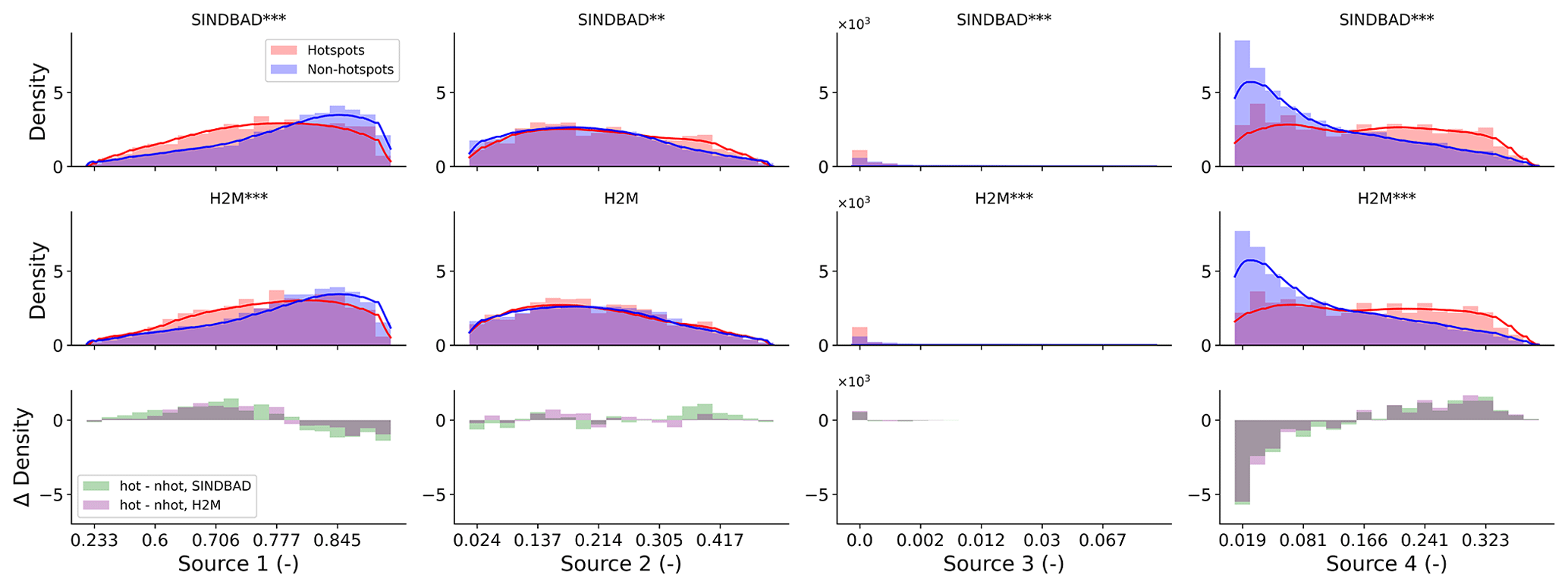
We find that the probability of vegetation accessing the secondary moisture is much larger in the error hotspots of TWS IAV. In particular, this association is stronger when the secondary groundwater moisture is coming from the upstream regions (source 4; Fig. 8). The hotspot occurrences are larger in regions where the primary source of moisture only supports a relatively smaller fraction of transpiration (source 1; Fig. 8). A larger fraction of transpiration here, therefore, may be supported by secondary and non-trivial sources. We find that the difference between the occurrences of error hotspots and non-hotspots is small in regions where transpiration is dependent on locally recharged groundwater (i.e., source 3). On the other hand, the difference is clearer in the regions where transpiration is supplied by remotely recharged groundwater (i.e., source 4).

Figure 8Same as Fig. 7 but for the contribution of four water sources to the water usage by vegetation. Data by Miguez-Macho and Fan (2021) were used for the four sources. Source 1 is soil water from recent (<1 month) precipitation, source 2 is soil water from past precipitation, source 3 is locally recharged groundwater via capillary flow, and source 4 is remotely recharged groundwater from uplands to lowlands.
Getting back to the three research questions, we first discuss the regions contributing most to the global TWS IAV and its modeling error (Sect. 4.1), and then, finally, we discuss potential sources of the error (Sect. 4.2).
4.1 Spatial contributions to the global TWS IAV and its error
The semi-arid regions are the main contributors to the variance in the global TWS IAV (Fig. 3), which agrees with the findings of previous studies. For example, Humphrey et al. (2018) showed a similarly large role of semi-arid regions in the global TWS IAV but found that only GRACE shows a large contribution from tropical regions. In that regard, the use of GRACE data in SINDBAD and H2M, perhaps, helps produce a regional and global pattern of TWS that is more consistent with GRACE than previously reported. As the semi-arid regions also have a dominant role in the IAV of the global terrestrial carbon sink (Poulter et al., 2014; Ahlstrom et al., 2015; Jung et al., 2017; Humphrey et al., 2018), the large contributions of semi-arid regions to the global TWS IAV imply a strong global-scale linkage between the water and carbon cycles (Law et al., 2002), as shown in Humphrey et al. (2018). But the role of the large TWS IAV contribution from humid tropical regions, which is prevalent in GRACE and the two data-driven models selected here, and its effect on the linkages of global water and carbon cycle still remains to be understood.
On the other hand, tropical regions come out as the dominant contributor to the variance in the global TWS IAV modeling errors (Fig. 4). Tropical regions were reported as being one significant contributor to the global TWS IAV but with a large disparity between the models and GRACE, (Humphrey et al., 2018) due, possibly, to the characteristics of the regions that the used models do not properly account for, e.g., artificial reservoirs, complex topography, or wetlands (Bolaños et al., 2021; Bolaños Chavarría et al., 2022). While SINDBAD and H2M mostly agree on the distribution of contributions, the two models show differences particularly in the semi-arid regions of southern Africa, where SINDBAD shows a negative contribution, while H2M shows a mostly positive contribution, resulting in a large positive difference between the models. The difference could possibly be attributable to whether a model considers the capillary rise (SINDBAD does and H2M does not) which changes the TWS dynamics, as vegetation can access and lose water as transpiration in the dry season (Guan et al., 2014; Madani et al., 2020; Miguez-Macho and Fan, 2021). In SINDBAD, vegetation indirectly accesses the secondary water storage with capillary rise, which contributes to a larger evapotranspiration over some regions, including the regions in Africa (Fig. 9 in Trautmann et al., 2022).
Generally, the model structure is an influential source of uncertainty in the distribution of hotspots. While SINDBAD and H2M cover the range of the model structure to a certain extent, other hydrological models may have a different distribution of hotspots and sources of errors. Following Kraft et al. (2022), among 10 global hydrological models (GHMs) in the eartH2Observe ensemble (Schellekens et al., 2017), we selected four GHMs with groundwater storage in the structure to identify the hotspots of TWS IAV modeling error, namely W3RA (Van Dijk and Warren, 2010), LISFLOOD (Van Der Knijff et al., 2010), SURFEX-TRIP (Decharme et al., 2010, 2013), and PCR-GLOBWB (van Beek et al., 2011; Wada et al., 2014). In Fig. B15, the four GHMs show strong positive contributions in the humid regions of northern South America (as SINDBAD and H2M do), but the four models disagree with SINDBAD and H2M for some regions like hotspots in central Africa. However, as different sets of forcing and constraints with different spatiotemporal domains were used for the simulation of the four GHMs and given the more complex structure of GHMs, further research will be required to investigate the hotspots and identify sources of TWS IAV modeling errors in each GHM.
4.2 Potential sources of errors
In the comparison of the TWS IAV and precipitation IAV time series within selected SREX regions in error hotspots, we find that modeled TWS IAV is more tightly correlated with precipitation IAV than GRACE TWS IAV is (Fig. 6). The consistently quicker response of the TWS IAV in the models points to either a lack of (1) sub-pixel and across-pixel moisture convergences or (2) insufficient representation of delayed storage, which is either simply represented in SINDBAD or ignored in H2M. The inferences were well supported by the characteristics of the error hotspots such as a larger river water storage, frequent occurrences of groundwater-driven wetlands, and a stronger contribution of groundwater recharged via the uplands-to-lowlands to transpiration (Figs. 7 and 8). The error hotspots are located in regions with a large potential for the lateral flow of surface water, e.g., regions with a well-developed river network (e.g., Amazon; as shown in Jung et al., 2010), or with a large accumulation of snowmelt in spring (e.g., Laurentian Great Lakes basin; as shown in Xiao et al., 2016; Huziy and Sushama, 2017). In these regions, the lateral flow delays the responses of the TWS to precipitation (Soni and Syed, 2015), effectively nullifying their correlation, as seen in the GRACE observation. The lack or underrepresentation of surface or delayed water dynamics is pointed out as being a critical improvement needed for the future (Kraft et al., 2022). SINDBAD represents a conceptually lumped delayed water storage (i.e., groundwater and surface water) using a state variable, wSlow. The wSlow variable has an unlimited storage capacity that depends on a globally constant model parameter, but it does not have spatiotemporal variability. Therefore, the lumped wSlow representation may not be sufficient to reproduce the globally varying but locally relevant large contribution of surface water storage to TWS IAV (e.g., Kim et al., 2009; Frappart et al., 2012; Getirana et al., 2017; Pokhrel et al., 2018; Schrapffer et al., 2020).
It has been reported that the water storage with delaying processes is relevant to the regional and global hydrology. River storage explains up to 73 % of the TWS variability in the Amazon (Kim et al., 2009). River routing affects the water flow patterns (Jung et al., 2010) and variability in simulated runoff (Jin et al., 2022). Improvements in the TWS simulations have been reported in the Amazon, Africa, and India when river routing is considered in the model (Getirana et al., 2017). Humphrey et al. (2018) pointed out that models are limited in representing groundwater–surface water dynamics, e.g., in wetlands, which may have a slower or no response to climatic forcings. The lack of slow water processes such as lateral flow will cause errors in simulating the hydrological cycle and will furthermore result in errors in simulating interactions among cycles, such as the water–carbon cycle interactions (Humphrey et al., 2018; Madani et al., 2020).
Other than the difference in the strength of correlation, models also do not capture some peaks of TWS IAV in the error hotspots. When there is missing water storage in the models, for example, the floodplain storage may be related to a smaller accumulation and lower positive anomaly than seen in GRACE, as also reported previously (Scanlon et al., 2018) and as the error hotspots have larger river water storage than non-hotspots (Fig. 7). The underestimation of the negative peaks may also be related to the use of a small soil water storage capacity in the models, which would not allow for a depletion of deeper moisture storage in infrequent but significant drought years. The soil water storage capacity in SINDBAD is mostly less than 2 m (Fig. B16), and Swenson and Lawrence (2015) reported that soil water storage capacity of 8–10 m is required to replicate the TWS variability over tropical regions observed by GRACE. However, the storage capacity is probably not the only reason, as H2M, which does not predefine soil water storage capacity, shows similar underestimations.
The error hotspots were also more prevalent in regions where the transpiration is significantly supported by the secondary moisture sources, especially the one from non-local groundwater recharge (Miguez-Macho and Fan, 2021). Even though SINDBAD accounts for the groundwater usage by vegetation, both the selected models show very similar distributions of the reliance, probably because SINDBAD also only represents the local recharge process. As the local distribution of groundwater recharge is prevalent at the hillslope scale, the remotely recharged groundwater, calculated at 30 arcsec resolution, can be interpreted as a sub-pixel-scale process for the spatial resolution of 1∘ used in the selected models. The missing sub-pixel convergence of moisture and its effect on water availability and on supporting ET would result in a bias in the ET simulations in the selected models, which would consequently translate to erroneous TWS. Indeed, we find that the selected models underestimate the ET compared to FLUXCOM observations (Fig. B17). On the other hand, the two models do not show a clear pattern with biases in the runoff (i.e., sub-pixel lateral flow) simulation. This suggests that, in some regions, the local redistribution of moisture and its effect on TWS variability is modulated by evapotranspiration rather than runoff processes.
Last, the additional sources of errors include (1) anthropogenic influence, (2) uncertainties in the GRACE and forcing data, and (3) model structure. Though the analysis excludes pixels with a large anthropogenic influence on TWS, such as northern India, following Rodell et al. (2018), some regions may still include the anthropogenic influence. In Africa, a decrease in TWS IAV in 2003–2006 (Fig. 6c) was due to the expansion of the Nalubaale Dam and La Niña (Stager et al., 2007; Awange et al., 2013, 2019). In the Indian subcontinent (Fig. 6d), the TWS changes have been reported due to human impacts such as reducing groundwater abstraction and surging reservoirs in addition to increased precipitation (Meghwal et al., 2019; Munagapati et al., 2021). Furthermore, the error hotspots include regions around typical irrigation-dominated areas such as the Corn Belt in the USA and northern India (Fig. 4). Note that most of these regions were excluded in the analysis of model simulations (Kraft et al., 2022; Trautmann et al., 2022), and trends were removed from all data and simulations to focus on the interannual variability in TWS under natural conditions. Regarding the GRACE errors, the GRACE mascon solution has the leakage error created during spatial interpolation from the original spatial resolution (3∘) to a higher resolution (0.5∘) (Wiese et al., 2016). Additionally, the Laurentian Great Lakes, which are visible as error hotspots, are also known to be in the effect of the post-glacial rebound (Peltier et al., 2015). The glacial isostatic adjustment is the major source of error in GRACE signal processing (Rodell et al., 2018). In addition, we note that the main findings of our study do not change even if a different GRACE mascon product was used, e.g., one from the Center for Space Research (CSR) (Save et al., 2016). JPL GRACE mascon and CSR GRACE mascon are qualitatively comparable to each other across global basins and at the interannual scale in addition to longer-term temporal scales (Scanlon et al., 2016). The two GRACE products are also largely consistent with each other in terms of the hotspots of the dynamics of global TWS IAV (Fig. B18).
With respect to the uncertainty from forcing and the model structure, we show that the use of different precipitation products does not significantly alter the main results and findings of the study (Figs. B19–B23), which was shown in Kraft et al. (2022) as well. In addition, the potential effect of the model structure is large. We assume that the two different models used in this study cover that source of uncertainty to a certain extent. Interestingly, we found that both models, which have vastly different model structures, showed a large consistency in the findings. Despite showing and presenting the effects of each of these factors separately, we cannot pinpoint and directly compare the uncertainty due to the input and the model structure, especially based on what is presented in the current work. For such an analysis, one would envisage a comprehensive factorial analysis of different modeling structures and the use of different input data but within a consistent model–data integration framework.
We provide a comprehensive application of a covariance matrix method that is effective for attributing global variability to each pixel. The method provides a platform to compare the magnitude and direction of the contribution of a single pixel or regions comprising arbitrary groups of pixels, owing to the normality and additive properties of the resulting statistic. Using this method, we quantified the contribution of each pixel to the global TWS IAV of GRACE observations and two selected predominantly data-driven models, SINDBAD and H2M, in addition to the modeling errors.
We found that the global TWS IAV is mainly driven by humid tropical and semi-arid regions. On the other hand, we identified the hotspots of the modeling errors in the global TWS IAV as being mainly in tropical regions that span across climatic regions. These different driving regions for the global TWS IAV and its errors show that the regions that dominate global TWS IAV are not necessarily the same as those that dominate the error in global TWS IAV. This allowed for a further analysis to identify the error hotspots and potential missing mechanisms in the models. Interestingly, we found that the largest 10 % error contributors explain 70 % of the global error, showing a disproportionately large significance of a small region in influencing the global mismatch with the observations.
Using the error hotspots as the basis for comparison, the TWS precipitation IAVs have a stronger correlation in the models than in the observation. This suggests different temporal dynamics of TWS and precipitation in the observations that are not captured by the models due to missing representations of key hydrological processes in some regions, which are congregated locally across different climates but still have a large influence on global errors. In fact, by associating them with hydrological variables, we found that the error hotspots are regions with larger river storage, lateral flow, and greater contribution of lateral flow to transpiration via recharging groundwater, which points to critical but missing processes of runoff accumulation, storage dynamics, and roles of secondary moisture in evaporative processes.
Our findings provide an improved understanding of the global TWS IAV and its modeling error. The models can be improved for global TWS IAV by focusing on the subgrid heterogeneity of moisture convergence and lateral flow processes that dominate the error hotspot regions. We also highlight the risk of inferring general process attributions and causations using global associations between variables, as only a small fraction of pixels may have significant implications of interannual variabilities at the global scale.
The forcing variables included precipitation, air temperature, and net radiation, and these were retrieved from GPCP V1DD V1.3 (Huffman et al., 2001), CRU JRA V2.2 (Harris, 2021), and CERES SYN1deg(Ed4A) (Wielicki et al., 1996), respectively. Four observational data streams were used to constrain both models, including (1) TWS from the Gravity Recovery and Climate Experiment (GRACE) Mascon Ocean, Ice, and Hydrology Equivalent Water Height Release 06 Coastal Resolution Improvement (CRI) Filtered Version 1.0 (Wiese et al., 2016), (2) snow water equivalent (SWE) from the GlobSnow v3 (Luojus et al., 2021), (3) evapotranspiration from the FLUXCOM v1 RS ensemble (Jung et al., 2019), and (4) runoff from the Global RUNoff ENSEMBLE (G‐RUN ENSEMBLE) v1 (Ghiggi et al., 2021). Note that vegetation characteristics such as the vegetation index and maximum rooting depth were only used for SINDBAD, while time-static land surface characteristics such as soil properties and wetland fractions were only used for H2M. See Trautmann et al. (2022) and Kraft et al. (2022) for the details of SINDBAD and H2M, respectively.
All forcing and constraints were aggregated into the 1∘ spatial resolution using the land area of each pixel; SWE was aggregated to the monthly scale. For GRACE, the original data have an irregular time step and occasionally have two observations within a month, with a missing value for the previous or next month. There are 2 months (January 2012 and April 2015) that have two observations for the study period (April 2002–June 2017), matching that of GRACE data. The earlier observation in January 2012 was regarded as an observation in December 2011, and the later observation in April 2015 was regarded as an observation in May 2015. The scaling factor was applied before the spatial aggregation. Gaps in the time series of each pixel were not filled, and all extrema were assumed to be a reasonable signal and included in the analysis. The GlobSnow SWE was spatially gap-filled to zero values in non-snow regions to obtain the global coverage, following Kraft et al. (2022). For the FLUXCOM ET, only a part of the study period was available (2002–2015). Last, the two models covered different land pixels due to independent data filtering (Kraft et al., 2022; Trautmann et al., 2022). The data filtering excludes land pixels with (1) a significant fraction of ice, snow, waterbody, bare land surface, or artificial land cover or (2) a large human influence on the trend in GRACE TWS, mainly by groundwater extraction, to reduce biases during calibration due to processes that models do not properly consider. For example, pixels with significant ice cover were excluded, as glacier changes considerably contribute to TWS, and especially its trend (Rodell et al., 2018; Scanlon et al., 2018), in the high latitudes of the Northern Hemisphere. Only the common land pixels between two model simulations were used in this analysis, and the same land mask was applied to all forcing and constraints.
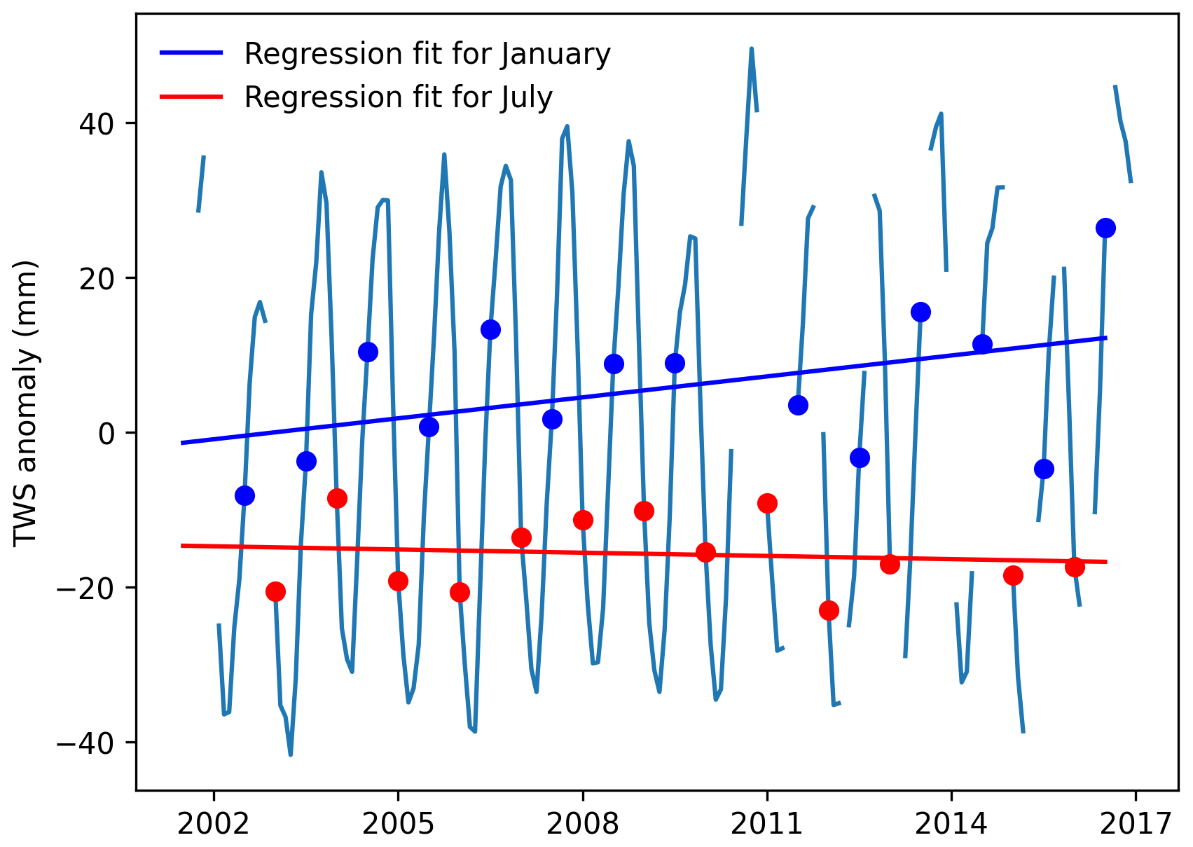
Figure B1Illustration of the calculation of interannual variability for the global terrestrial water storage (TWS) anomalies.
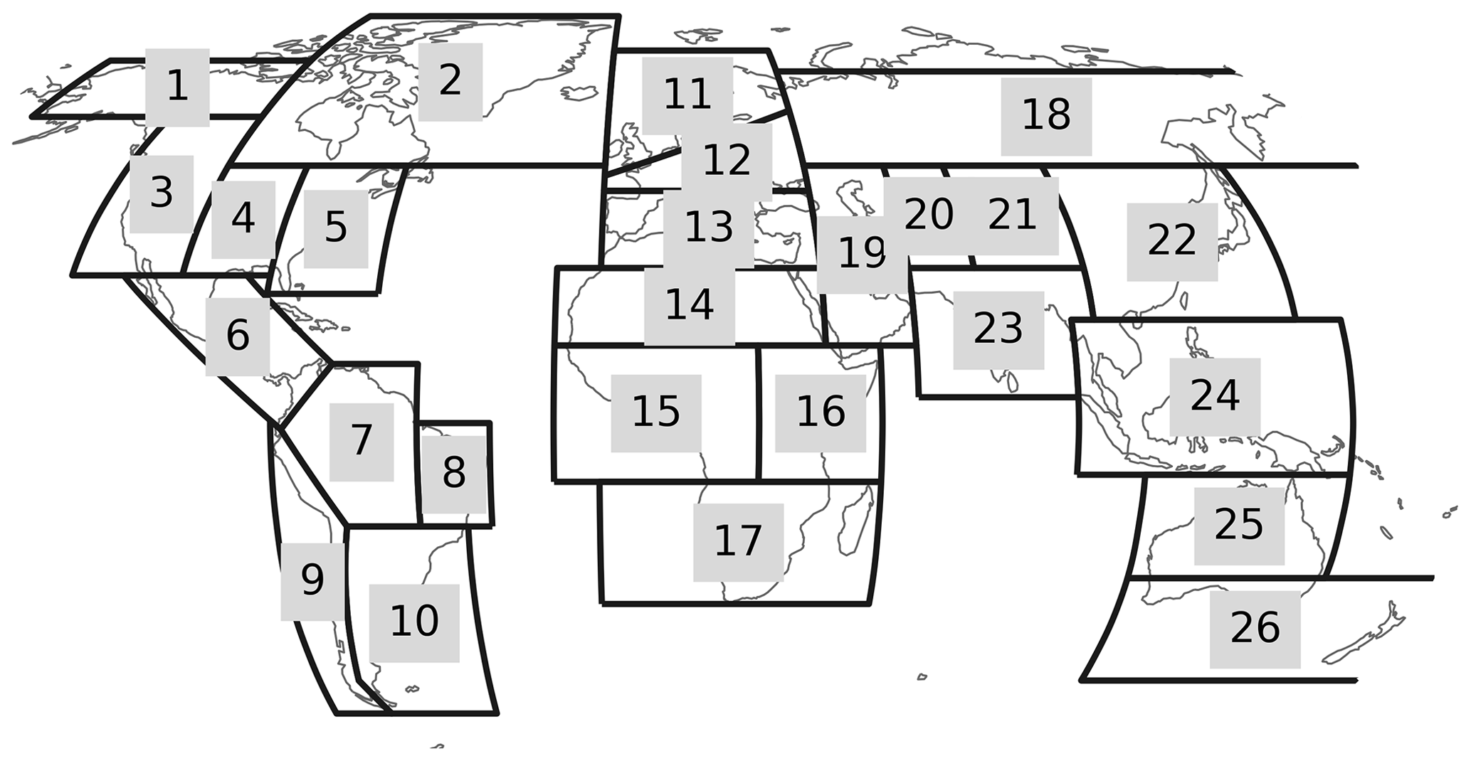
Figure B2The Intergovernmental Panel on Climate Change (IPCC) Special Report on Extremes (SREX) regions (Seneviratne et al., 2012), which were used in the figures (Figs. 6, B6, and B9–B11) to spatially average the global terrestrial water storage interannual variability time series into four selected regions. These include the Laurentian Great Lakes (SREX regions 5), the Amazon (SREX regions 7), eastern and western Africa (SREX regions 15 and 16), and South Asia (SREX regions 23).
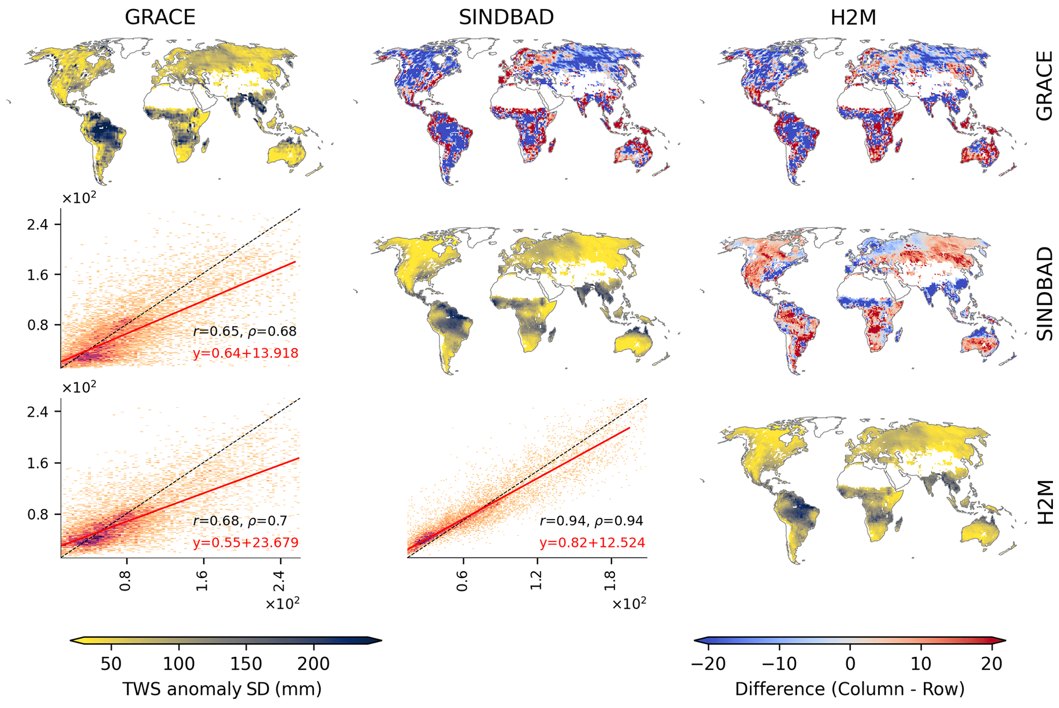
Figure B3Same as Fig. 3 but for the standard deviation (SD) of the global terrestrial water storage (TWS) anomalies instead of the pixel-wise contributions to the variance in the global TWS interannual variability.
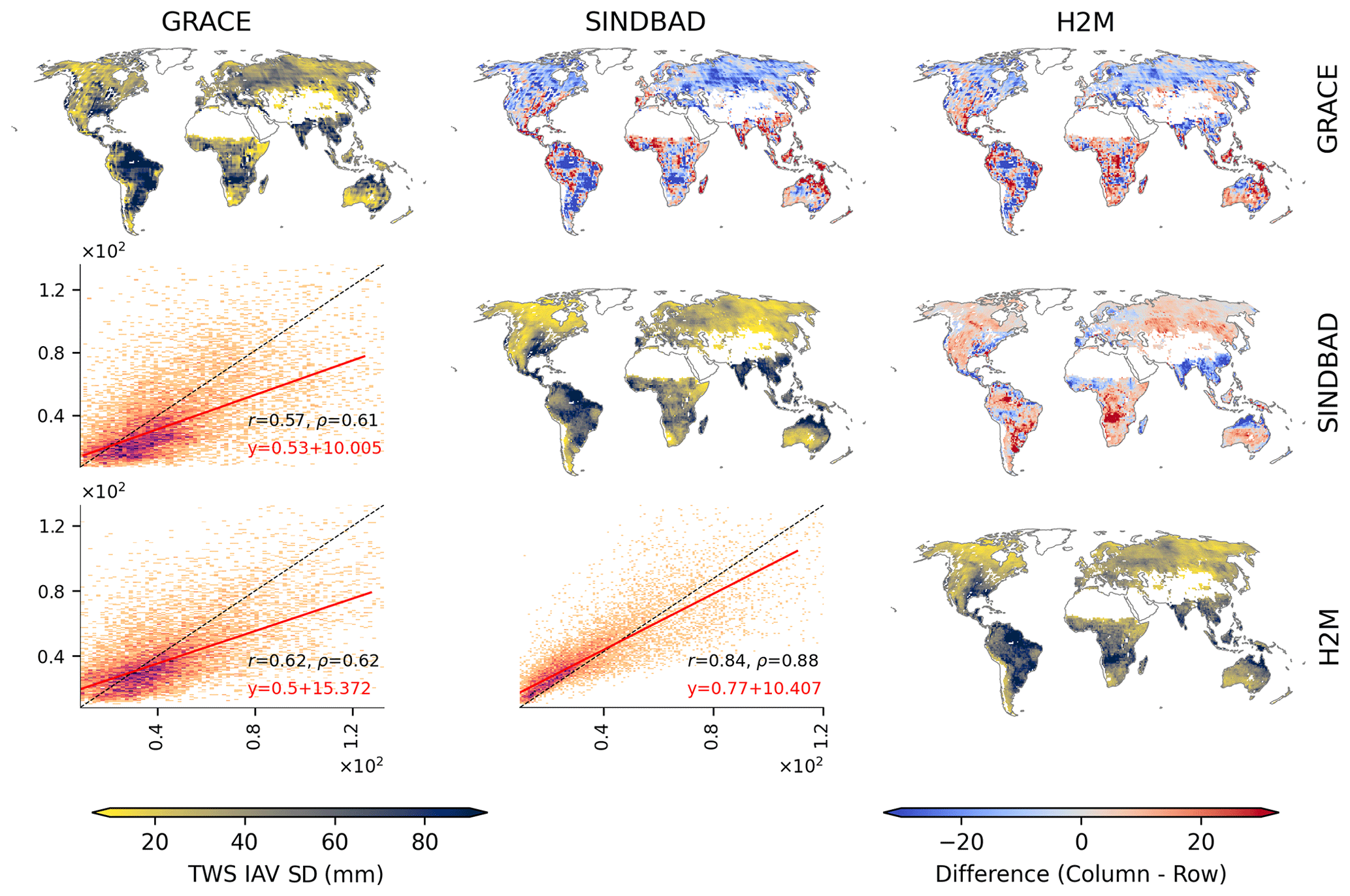
Figure B4Same as Fig. 3 but for the standard deviation (SD) of the global terrestrial water storage (TWS) interannual variability (IAV) instead of the pixel-wise contributions to the variance in the global TWS IAV.
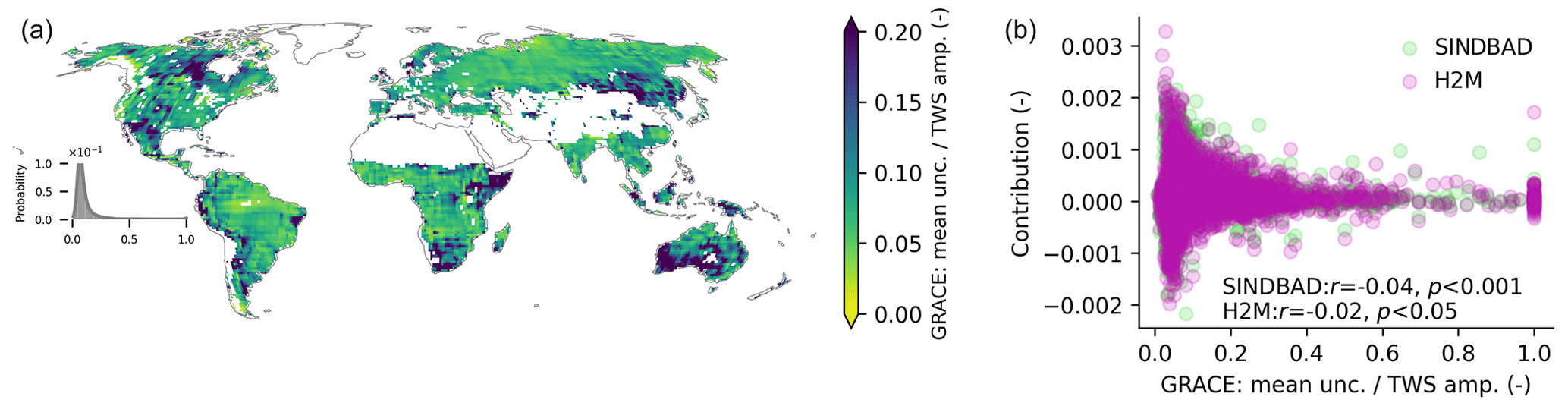
Figure B5(a) Spatial distribution of the relative uncertainty in GRACE terrestrial water storage (TWS) observations. The relative uncertainty in each pixel is calculated as the mean uncertainty divided by the amplitude of TWS. (b) Scatterplots comparing the relative uncertainty in GRACE TWS (x axis) versus pixel-wise contributions to the global TWS IAV modeling error (y axis). Shown below as text is the Pearson correlation coefficient with the p value of each model.
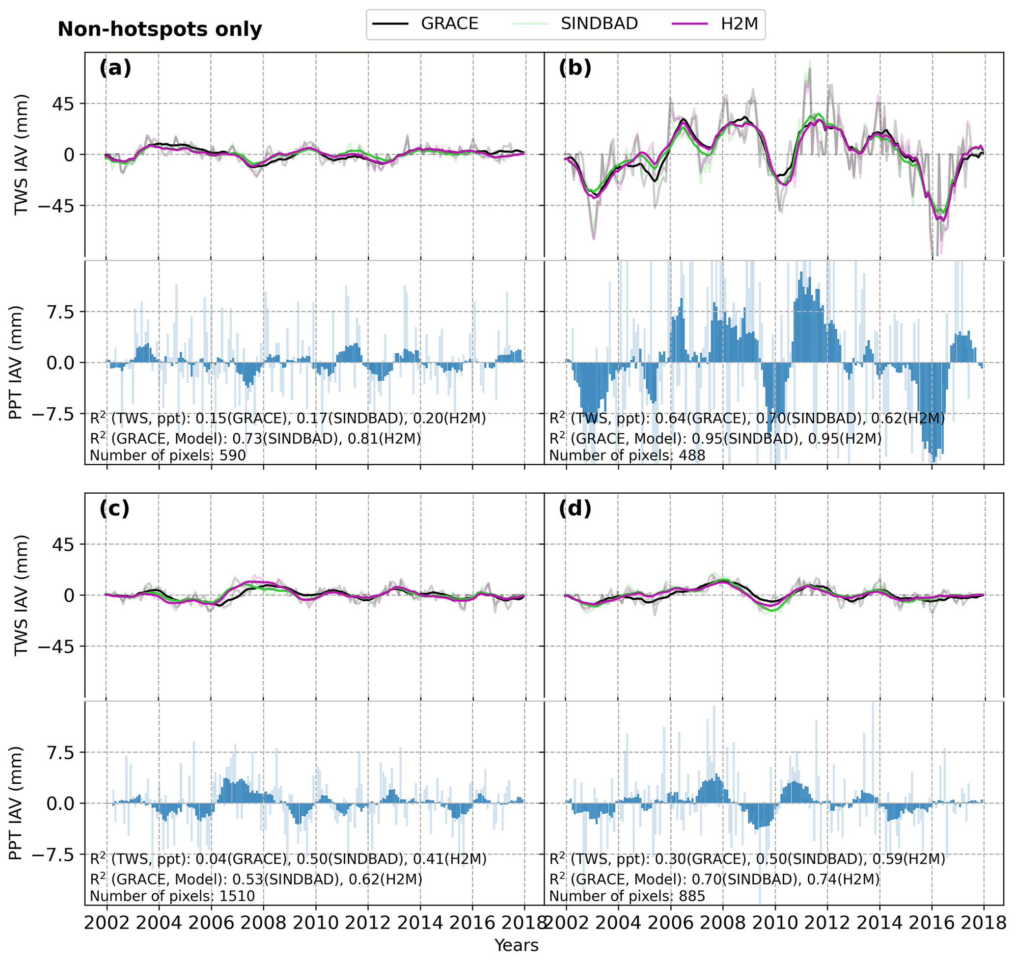
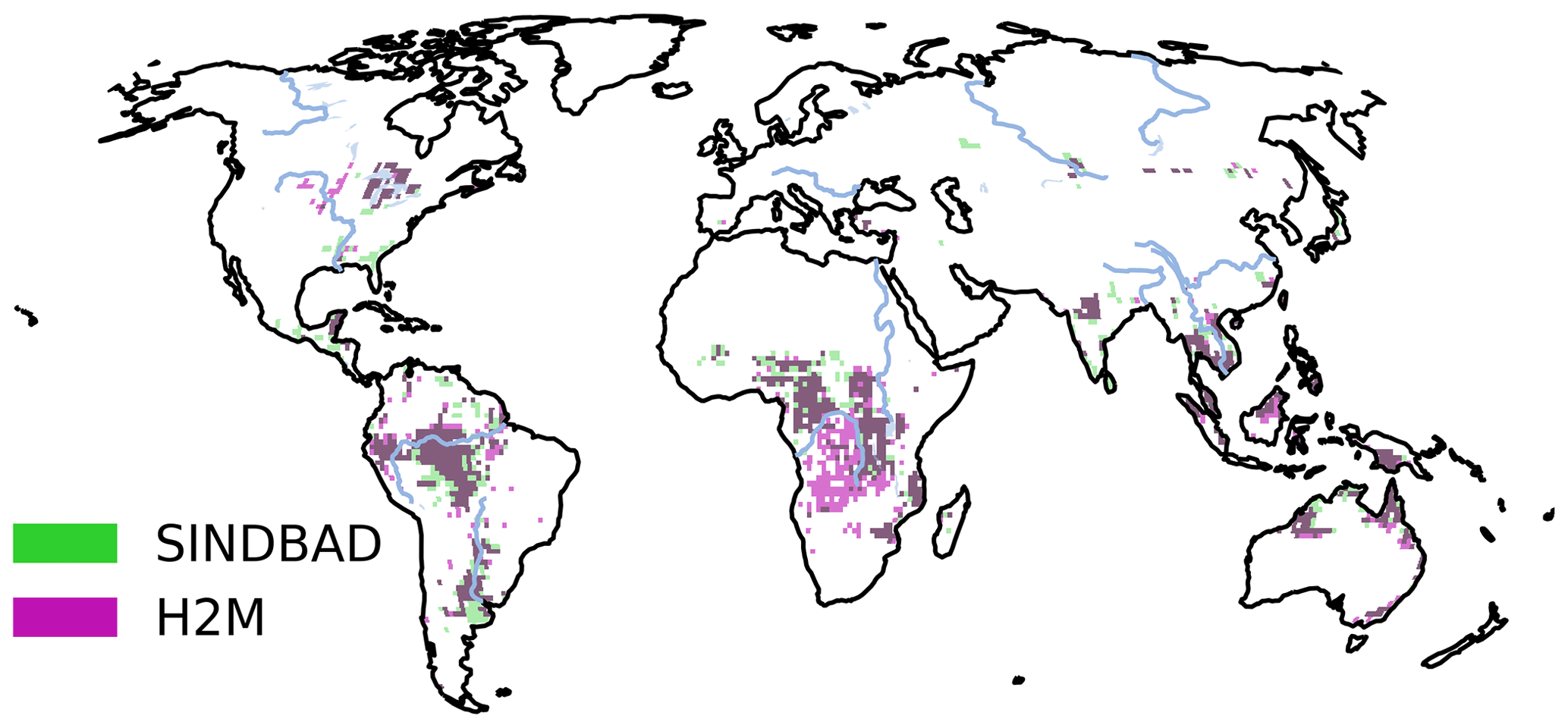
Figure B7Spatial patterns of error hotspots of modeling errors in terrestrial water storage (TWS) interannual variability (IAV). Error hotspots mean pixels with 10 % of the largest positive contributions to the global TWS IAV modeling errors (Fig. 4). Red pixels are error hotspots identified using SINDBAD, light purple pixels are error hotspots identified using H2M, and dark purple pixels are commonly identified error hotspots by the two models.
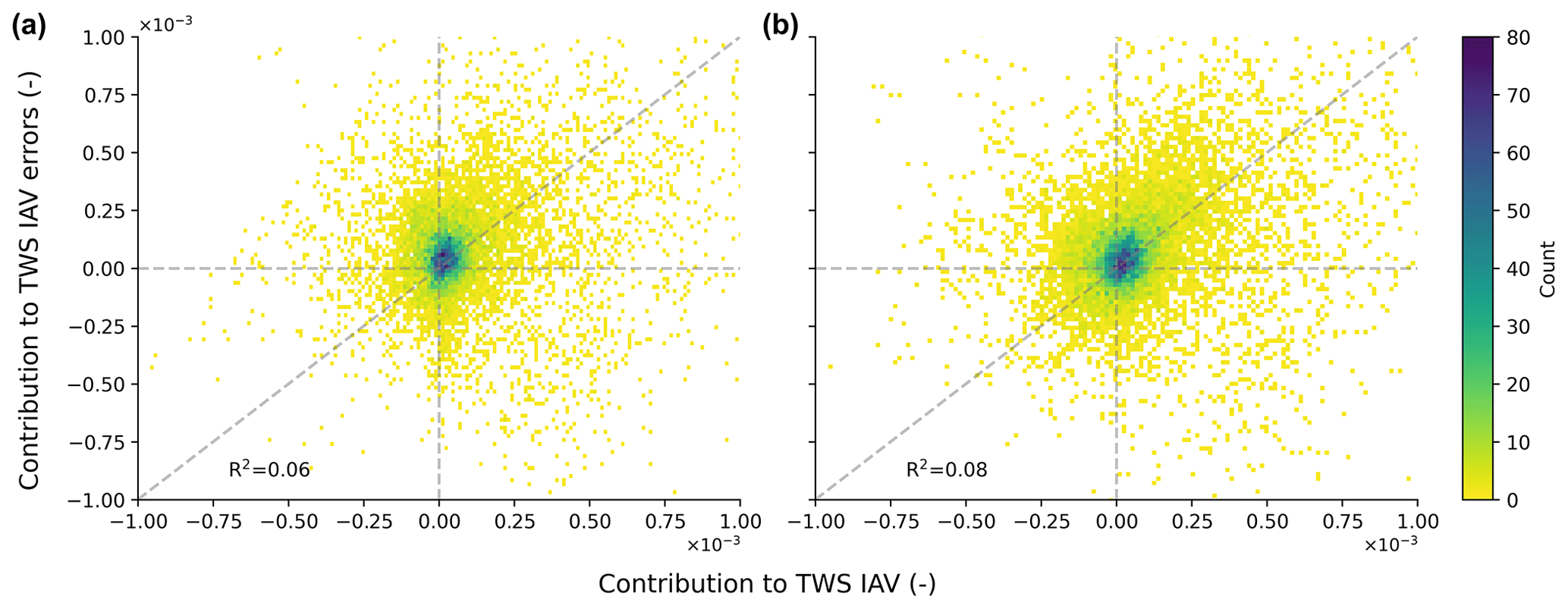
Figure B8Bivariate histograms that compare the pixel-wise contribution to the global terrestrial water storage (TWS) interannual variability (IAV) versus pixel-wise contributions to the global TWS IAV modeling error in SINDBAD (a) and H2M (b). The pixel-wise contribution is quantified using Eq. (4) (see Sect. 2.1.2). Colors mean the number of cases with corresponding ranges of contribution to TWS IAV and contribution to TWS IAV errors. R2 at the bottom left is calculated as the square of the Pearson correlation coefficient.
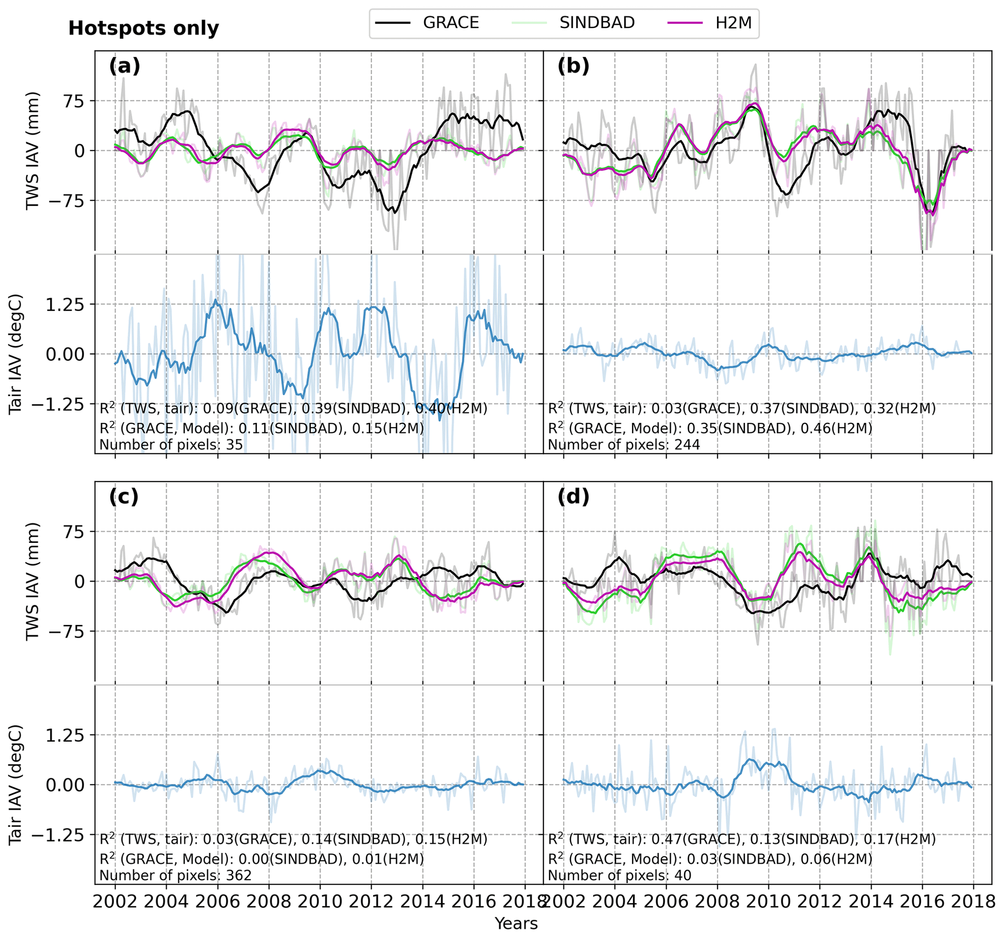
Figure B9Same as Fig. 6 but using air temperature (Tair) IAV instead of precipitation (PPT) IAV.
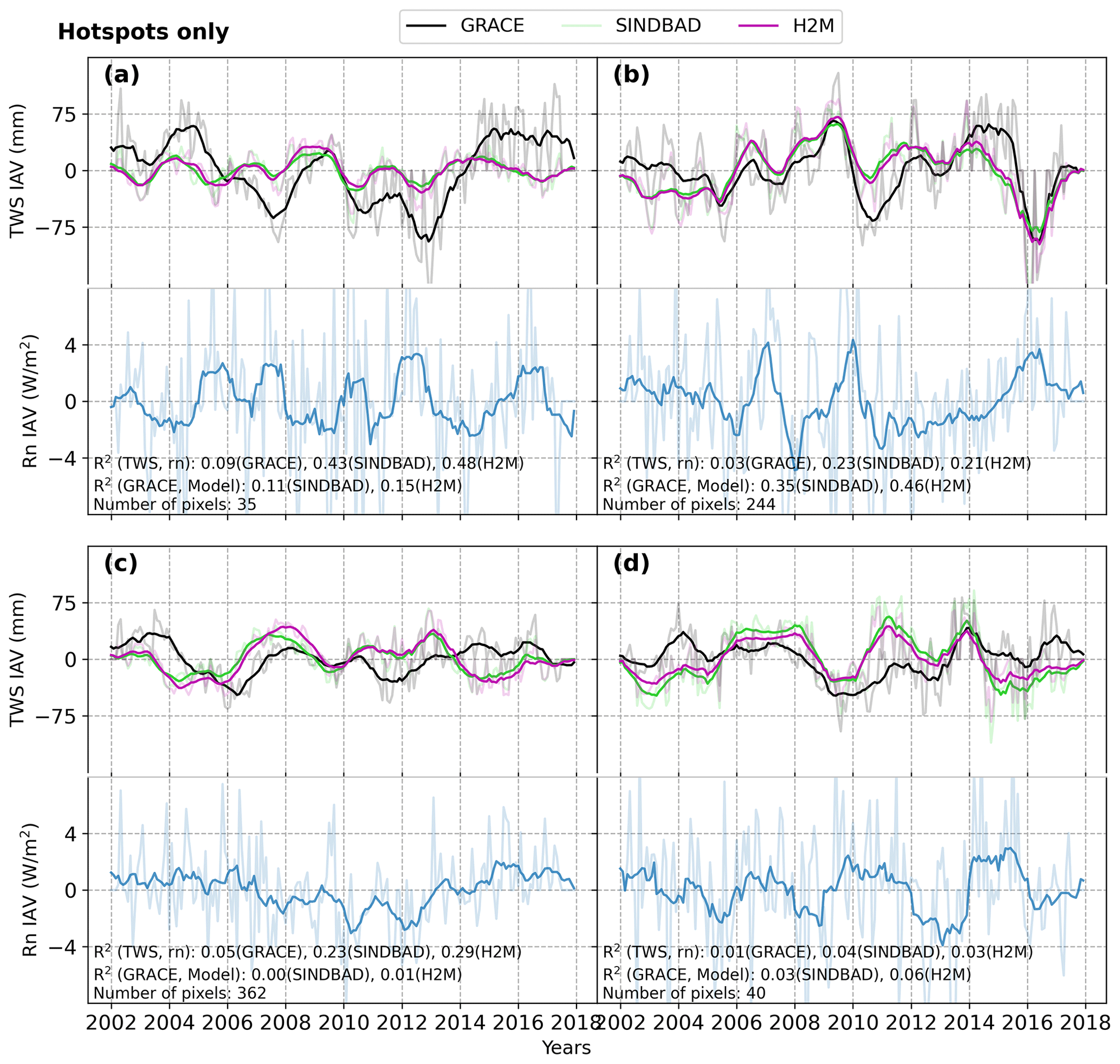
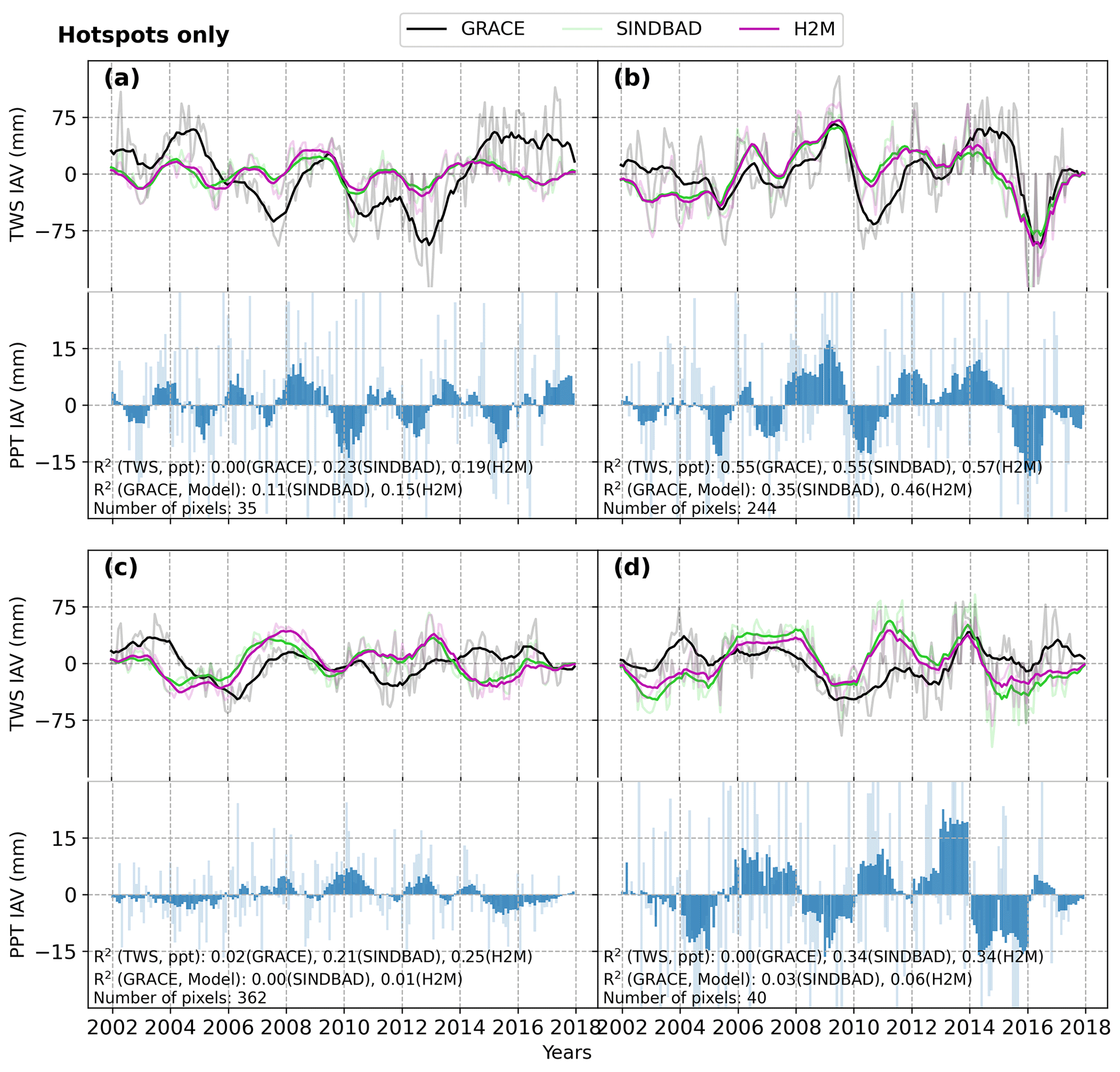
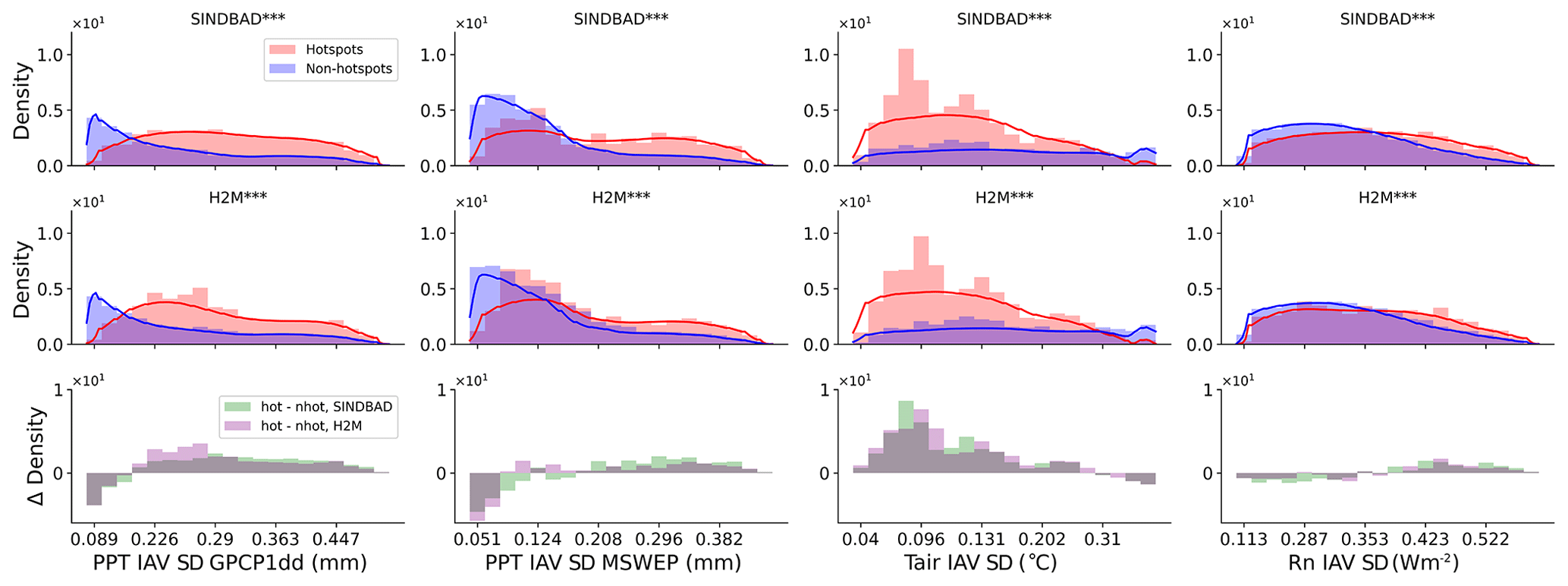
Figure B12Same as Fig. 7 but for meteorological forcing variables, including the standard deviation (SD) of precipitation (PPT), interannual variation (IAV), air temperature IAV SD, and net radiation (Rn) IAV SD. The first two columns from the left show results using different PPT data sets (GPCP1dd and MSWEP).
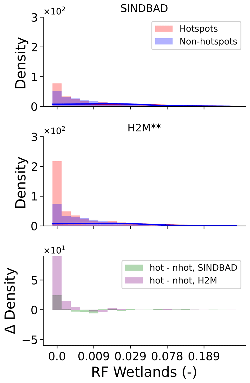
Figure B13Same as Fig. 7 but for the fraction of regularly flooded (RF) wetlands provided by Tootchi et al. (2019).
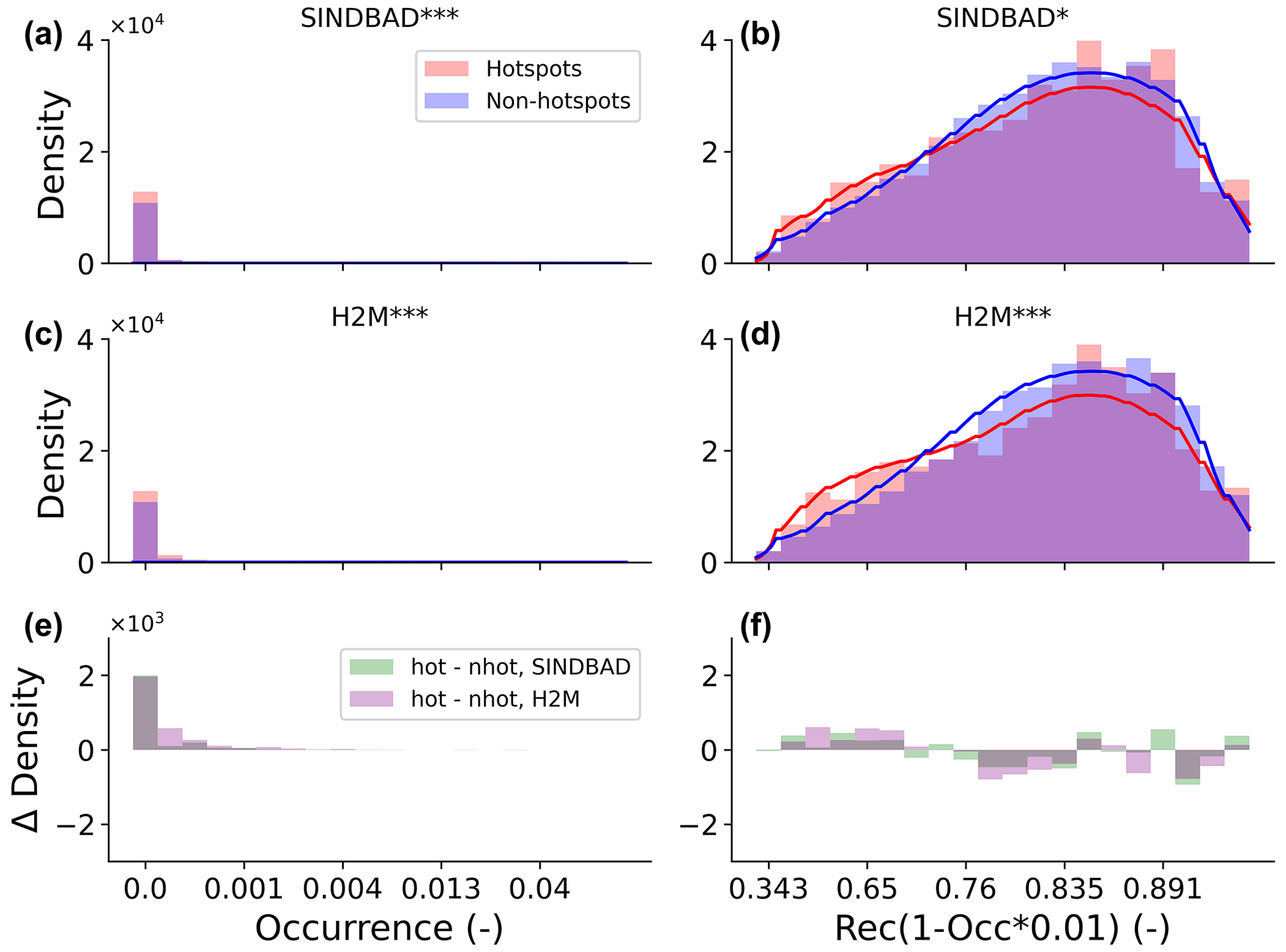
Figure B14Same as Fig. 7 but using the occurrence (a, c, e) and the product of the recurrence and occurrence (b, d, f) of the surface waterbodies from the global surface water explorer data set (GSWE; Pekel et al., 2016).
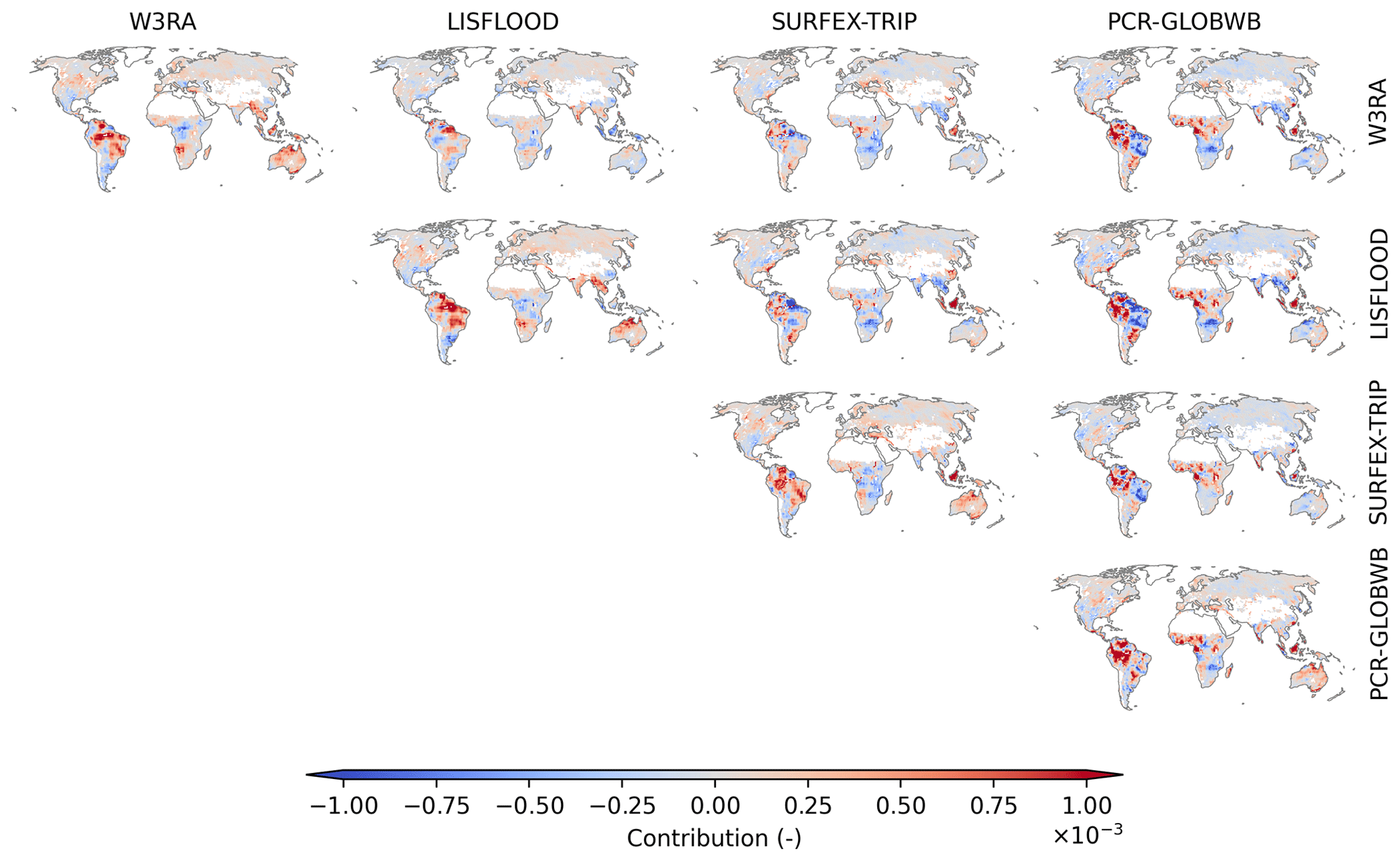
Figure B15Global distribution of pixel-wise contributions to the variance in the modeling error in global terrestrial water storage interannual variability by selected global hydrological models from the eartH2Observe ensemble (Schellekens et al., 2017). Along the diagonal, maps of the pixel-wise contribution to the global TWS IAV modeling errors in W3RA, LISFLOOD, SURFEX-TRIP, and PCR-GLOBWB are shown. Above the diagonal, a map of the difference (i.e., column−row) is shown. For example, the map of the first row and the second column is for LISFLOOD (column) minus W3RA (row). White pixels within land boundaries are the regions masked out in this study (see Appendix A).
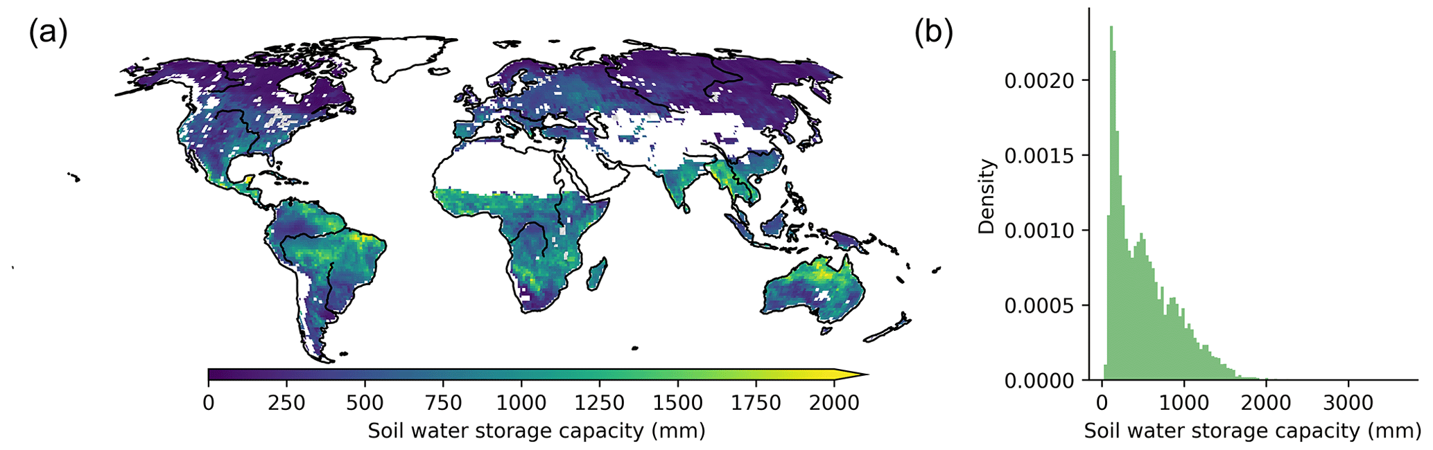
Figure B16Spatial distribution (a) and histogram (b) of the soil water storage capacity of SINDBAD shown as the sum of the capacity of two soil layers.
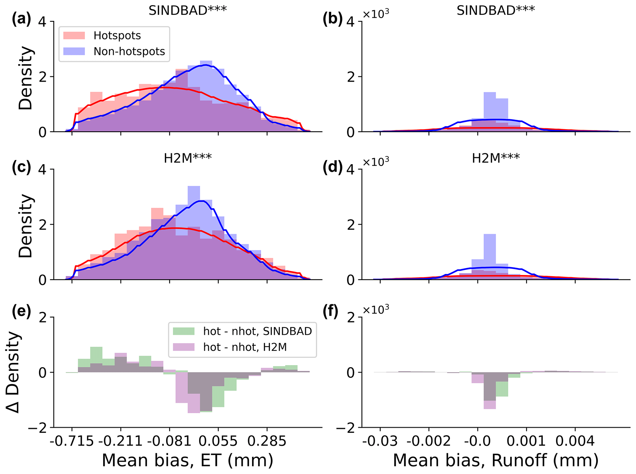
Figure B17Same as Fig. 7 but for the mean bias in evapotranspiration (ET; a, c, e) and runoff (b, d, f) simulations with two tested models. Note that the x axis is not in the normalized unit using the minimum and maximum but in the original unit.
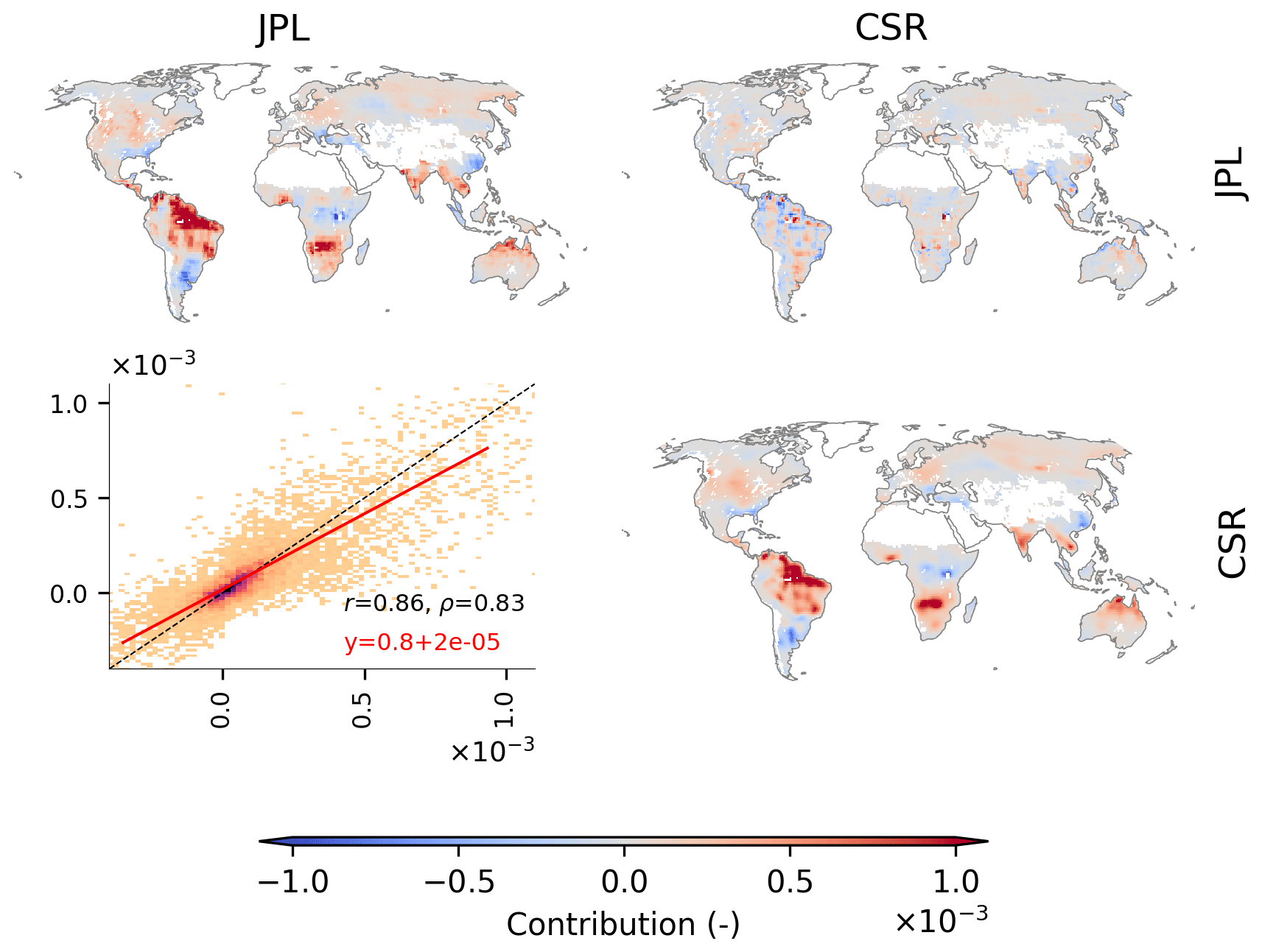
Figure B18Same as Fig. 3 but for two GRACE mascon products by the Jet Propulsion Laboratory (JPL) and the Center for Space Research (CSR).
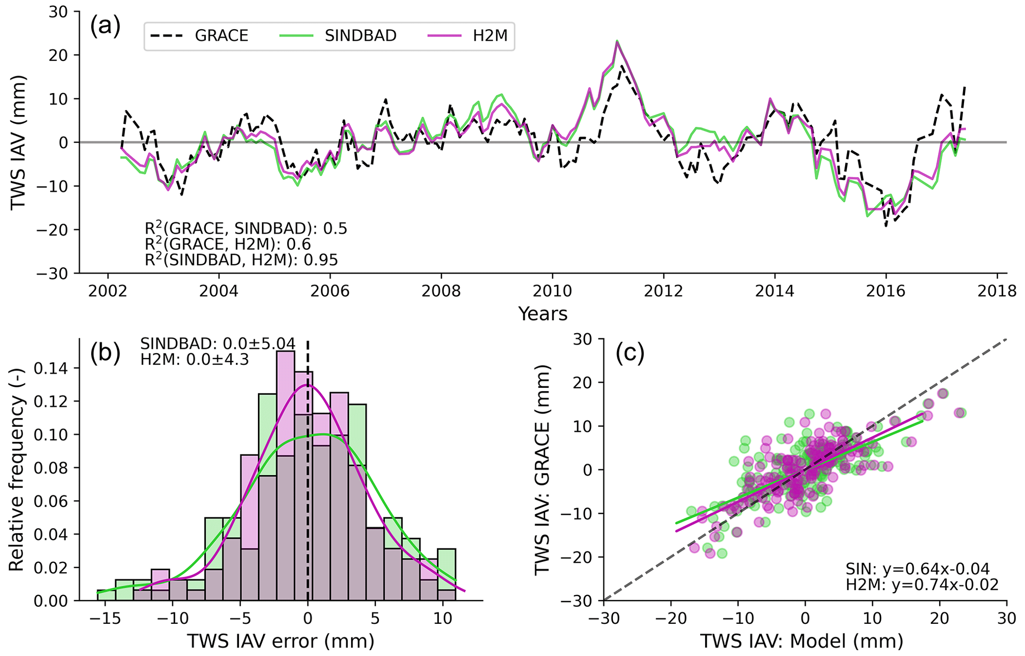
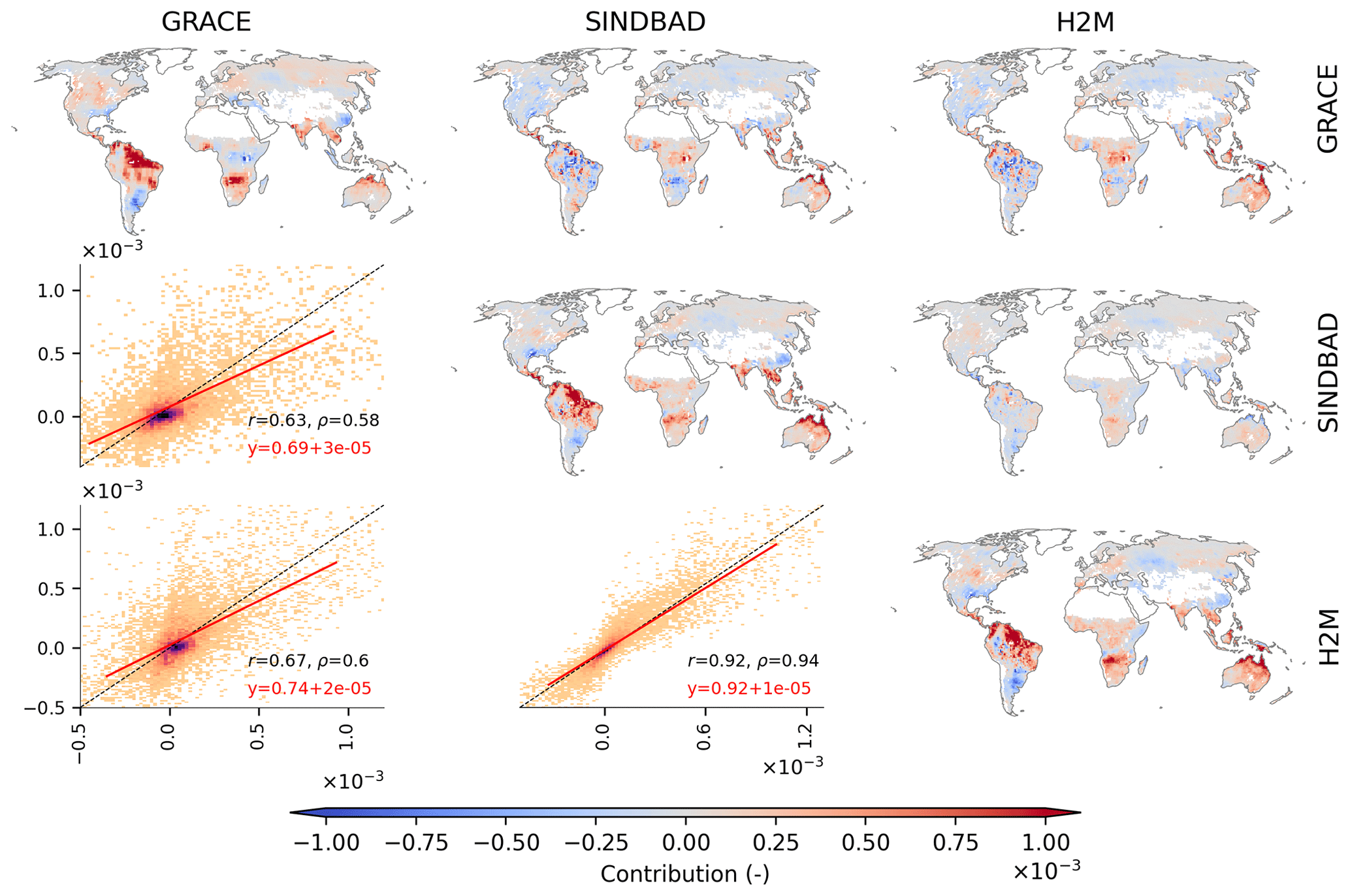
Figure B20Same as Fig. 3 but using MSWEP instead of GPCP1dd for the precipitation forcing.
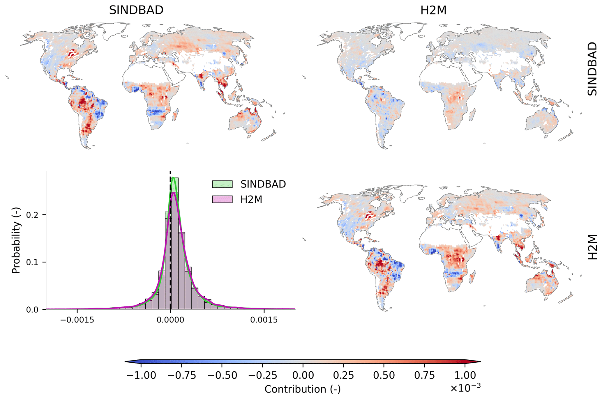
Figure B21Same as Fig. 4 but using MSWEP instead of GPCP1dd for the precipitation forcing.
The SINDBAD and H2M simulations and processed data sets are available at https://doi.org/10.5281/zenodo.7813179 (Lee et al., 2023a). The Python scripts for the analyses and for producing the figures can be accessed via a public repository on GitHub (https://github.com/hoontaeklee/hlee_tws_iav_hotspots; Lee et al., 2023b).
MJ, SK, and HL designed the experiments. TT and BK performed the model simulations. In close collaboration with SK, HL conducted the analysis and prepared the first draft. All authors contributed to the research discussions and improving the paper.
The contact author has declared that none of the authors has any competing interests.
Publisher's note: Copernicus Publications remains neutral with regard to jurisdictional claims in published maps and institutional affiliations.
Hoontaek Lee acknowledges support from the Max Planck Institute for Biogeochemistry (MPI-BGC) and the International Max Planck Research School for Global Biogeochemical Cycles (IMPRS-gBGC). We also thank Uli Weber at MPI-BGC for the collection and preparation of the data used in the model simulations and analysis.
The article-processing charges for this open-access publication were covered by the Max Planck Society.
This paper was edited by Yue-Ping Xu and reviewed by Silvana Bolaños and two anonymous referees.
Ahlstrom, A., Raupach, M. R., Schurgers, G., Smith, B., Arneth, A., Jung, M., Reichstein, M., Canadell, J. G., Friedlingstein, P., Jain, A. K., Kato, E., Poulter, B., Sitch, S., Stocker, B. D., Viovy, N., Wang, Y. P., Wiltshire, A., Zaehle, S., and Zeng, N.: The dominant role of semi-arid ecosystems in the trend and variability of the land CO2 sink, Science, 348, 895–899, https://doi.org/10.1126/science.aaa1668, 2015. a
Awange, J. L., Anyah, R., Agola, N., Forootan, E., and Omondi, P.: Potential impacts of climate and environmental change on the stored water of Lake Victoria Basin and economic implications, Water Resour. Res., 49, 8160–8173, https://doi.org/10.1002/2013WR014350, 2013. a
Awange, J. L., Saleem, A., Sukhadiya, R. M., Ouma, Y. O., and Kexiang, H.: Physical dynamics of Lake Victoria over the past 34 years (1984–2018): Is the lake dying?, Sci. Total Environ., 658, 199–218, https://doi.org/10.1016/j.scitotenv.2018.12.051, 2019. a, b
Beck, H. E., Wood, E. F., Pan, M., Fisher, C. K., Miralles, D. G., v. Dijk, A. I. J. M., McVicar, T. R., and Adler, R. F.: MSWEP V2 Global 3-Hourly 0.1∘ Precipitation: Methodology and Quantitative Assessment, B. Am. Meteorol. Soc., 100, 473–500, https://doi.org/10.1175/BAMS-D-17-0138.1, 2019. a, b
Bolaños, S., Salazar, J. F., Betancur, T., and Werner, M.: GRACE reveals depletion of water storage in northwestern South America between ENSO extremes, J. Hydrol., 596, 125687, https://doi.org/10.1016/j.jhydrol.2020.125687, 2021. a
Bolaños Chavarría, S., Werner, M., Salazar, J. F., and Betancur Vargas, T.: Benchmarking global hydrological and land surface models against GRACE in a medium-sized tropical basin, Hydrol. Earth Syst. Sci. 26, 4323–4344, https://doi.org/10.5194/hess-26-4323-2022, 2022. a
Chapin, F. S., Matson, P. A., and Vitousek, P. M.: Water and Energy Balance, in: Principles of Terrestrial Ecosystem Ecology, edited by: Chapin, F. S., Matson, P. A., and Vitousek, P. M., Springer, New York, NY, 93–122, https://doi.org/10.1007/978-1-4419-9504-9_4, 2011. a
Chen, J. L., Wilson, C. R., and Tapley, B. D.: The 2009 exceptional Amazon flood and interannual terrestrial water storage change observed by GRACE, Water Resour. Res., 46, W12526, https://doi.org/10.1029/2010WR009383, 2010. a, b
Decharme, B., Alkama, R., Douville, H., Becker, M., and Cazenave, A.: Global Evaluation of the ISBA-TRIP Continental Hydrological System. Part II: Uncertainties in River Routing Simulation Related to Flow Velocity and Groundwater Storage, J. Hydrometeorol., 11, 601–617, https://doi.org/10.1175/2010JHM1212.1, 2010. a
Decharme, B., Martin, E., and Faroux, S.: Reconciling soil thermal and hydrological lower boundary conditions in land surface models, J. Geophys. Res.-Atmos., 118, 7819–7834, https://doi.org/10.1002/jgrd.50631, 2013. a
Famiglietti, J. S.: Remote Sensing of Terrestrial Water Storage, Soil Moisture and Surface Waters, in: The State of the Planet: Frontiers and Challenges in Geophysics, AGU – American Geophysical Union, 197–207, https://doi.org/10.1029/150GM16, 2004. a
Fan, Y., Li, H., and Miguez-Macho, G.: Global Patterns of Groundwater Table Depth, Science, 339, 940–943, https://doi.org/10.1126/science.1229881, 2013. a
Felfelani, F., Wada, Y., Longuevergne, L., and Pokhrel, Y. N.: Natural and human-induced terrestrial water storage change: A global analysis using hydrological models and GRACE, J. Hydrol., 553, 105–118, https://doi.org/10.1016/j.jhydrol.2017.07.048, 2017. a
Frappart, F. and Ramillien, G.: Monitoring Groundwater Storage Changes Using the Gravity Recovery and Climate Experiment (GRACE) Satellite Mission: A Review, Remote Sens., 10, 829, https://doi.org/10.3390/rs10060829, 2018. a
Frappart, F., Papa, F., d. Silva, J. S., Ramillien, G., Prigent, C., Seyler, F., and Calmant, S.: Surface freshwater storage and dynamics in the Amazon basin during the 2005 exceptional drought, Environ. Res. Lett., 7, 044010, https://doi.org/10.1088/1748-9326/7/4/044010, 2012. a
Getirana, A., Kumar, S., Girotto, M., and Rodell, M.: Rivers and Floodplains as Key Components of Global Terrestrial Water Storage Variability: Water Storage in Rivers and Floodplains, Geophys. Res. Lett., 44, 10359–10,68, https://doi.org/10.1002/2017GL074684, 2017. a, b
Ghiggi, G., Humphrey, V., Seneviratne, S. I., and Gudmundsson, L.: G-RUN ENSEMBLE: A Multi-Forcing Observation-Based Global Runoff Reanalysis, Water Resour. Res., 57, e2020WR028787, https://doi.org/10.1029/2020WR028787, 2021. a
Guan, K., Wood, E. F., Medvigy, D., Kimball, J., Pan, M., Caylor, K. K., Sheffield, J., Xu, X., and Jones, M. O.: Terrestrial hydrological controls on land surface phenology of African savannas and woodlands: Hydrology controls on African phenology, J. Geophys. Res.-Biogeo., 119, 1652–1669, https://doi.org/10.1002/2013JG002572, 2014. a, b
Harris, I.: CRU JRA v2.2: A forcings dataset of gridded land surface blend of Climatic Research Unit (CRU) and Japanese reanalysis (JRA) data; Jan. 1901–Dec. 2020, https://catalogue.ceda.ac.uk/uuid/4bdf41fc10af4caaa489b14745c665a6 (last access: 3 April 2023), 2021. a, b
Hosseini-Moghari, S.-M., Araghinejad, S., Ebrahimi, K., Tang, Q., and AghaKouchak, A.: Using GRACE satellite observations for separating meteorological variability from anthropogenic impacts on water availability, Sci. Rep., 10, 15098, https://doi.org/10.1038/s41598-020-71837-7, 2020. a
Huffman, G. J., Adler, R. F., Morrissey, M. M., Bolvin, D. T., Curtis, S., Joyce, R., McGavock, B., and Susskind, J.: Global Precipitation at One-Degree Daily Resolution from Multisatellite Observations, J. Hydrometeorol., 2, 36–50, https://doi.org/10.1175/1525-7541(2001)002<0036:GPAODD>2.0.CO;2, 2001. a, b
Humphrey, V., Gudmundsson, L., and Seneviratne, S. I.: Assessing Global Water Storage Variability from GRACE: Trends, Seasonal Cycle, Subseasonal Anomalies and Extremes, Surv. Geophys., 37, 357–395, https://doi.org/10.1007/s10712-016-9367-1 2016. a, b
Humphrey, V., Zscheischler, J., Ciais, P., Gudmundsson, L., Sitch, S., and Seneviratne, S. I.: Sensitivity of atmospheric CO2 growth rate to observed changes in terrestrial water storage, Nature, 560, 628–631, https://doi.org/10.1038/s41586-018-0424-4, 2018. a, b, c, d, e, f, g, h
Humphrey, V., Berg, A., Ciais, P., Gentine, P., Jung, M., Reichstein, M., Seneviratne, S. I., and Frankenberg, C.: Soil moisture–atmosphere feedback dominates land carbon uptake variability, Nature, 592, 65–69, https://doi.org/10.1038/s41586-021-03325-5, 2021. a
Huziy, O. and Sushama, L.: Impact of lake–river connectivity and interflow on the Canadian RCM simulated regional climate and hydrology for Northeast Canada, Clim. Dynam., 48, 709–725, https://doi.org/10.1007/s00382-016-3104-9, 2017. a
Jensen, L., Eicker, A., Dobslaw, H., Stacke, T., and Humphrey, V.: Long-Term Wetting and Drying Trends in Land Water Storage Derived From GRACE and CMIP5 Models, J. Geophys. Res.-Atmos., 124, 9808–9823, https://doi.org/10.1029/2018JD029989, 2019. a, b
Jensen, L., Eicker, A., Dobslaw, H., and Pail, R.: Emerging Changes in Terrestrial Water Storage Variability as a Target for Future Satellite Gravity Missions, Remote Sens., 12, 3898, https://doi.org/10.3390/rs12233898, 2020. a
Jin, J., Wang, L., Yang, J., Si, B., and Niu, G.-Y.: Improved runoff simulations for a highly varying soil depth and complex terrain watershed in the Loess Plateau with the Community Land Model version 5, Geosci. Model Dev., 15, 3405–3416, https://doi.org/10.5194/gmd-15-3405-2022, 2022. a
Jung, H. C., Hamski, J., Durand, M., Alsdorf, D., Hossain, F., Lee, H., Hossain, A. K. M. A., Hasan, K., Khan, A. S., and Hoque, A. Z.: Characterization of complex fluvial systems using remote sensing of spatial and temporal water level variations in the Amazon, Congo, and Brahmaputra Rivers, Earth Surf. Proc. Land., 35, 294–304, https://doi.org/10.1002/esp.1914, 2010. a, b
Jung, M., Reichstein, M., Schwalm, C. R., Huntingford, C., Sitch, S., Ahlström, A., Arneth, A., Camps-Valls, G., Ciais, P., Friedlingstein, P., Gans, F., Ichii, K., Jain, A. K., Kato, E., Papale, D., Poulter, B., Raduly, B., Rödenbeck, C., Tramontana, G., Viovy, N., Wang, Y.-P., Weber, U., Zaehle, S., and Zeng, N.: Compensatory water effects link yearly global land CO2 sink changes to temperature, Nature, 541, 516–520, https://doi.org/10.1038/nature20780, 2017. a, b, c
Jung, M., Koirala, S., Weber, U., Ichii, K., Gans, F., Camps-Valls, G., Papale, D., Schwalm, C., Tramontana, G., and Reichstein, M.: The FLUXCOM ensemble of global land-atmosphere energy fluxes, Scient. Data, 6, 74, https://doi.org/10.1038/s41597-019-0076-8, 2019. a
Kim, H., Yeh, P. J.-F., Oki, T., and Kanae, S.: Role of rivers in the seasonal variations of terrestrial water storage over global basins, Geophys. Res. Lett., 36, L17402, https://doi.org/10.1029/2009GL039006, 2009. a, b, c
Koirala, S., Yeh, P. J.-F., Hirabayashi, Y., Kanae, S., and Oki, T.: Global-scale land surface hydrologic modeling with the representation of water table dynamics, J. Geophys. Res.-Atmos., 119, 75–89, https://doi.org/10.1002/2013JD020398, 2014. a
Kraft, B., Jung, M., Körner, M., and Reichstein, M.: Hybrid Modeling: Modeling Fusion Of A Deep Learning Approach And A Physics-Based Model For Global Hydrological Modeling, Int. Arch. Photogramm. Remote Sens. Spatial Inf. Sci.,, XLIII-B2-2020, 1537–1544, https://doi.org/10.5194/isprs-archives-XLIII-B2-2020-1537-2020, 2020. a
Kraft, B., Jung, M., Körner, M., Koirala, S., and Reichstein, M.: Towards hybrid modeling of the global hydrological cycle, Hydrol. Earth Syst. Sci., 26, 1579–1614, https://doi.org/10.5194/hess-26-1579-2022, 2022. a, b, c, d, e, f, g, h, i, j, k, l, m, n, o
Law, B. E., Falge, E., Gu, L., Baldocchi, D. D., Bakwin, P., Berbigier, P., Davis, K., Dolman, A. J., Falk, M., Fuentes, J. D., Goldstein, A., Granier, A., Grelle, A., Hollinger, D., Janssens, I. A., Jarvis, P., Jensen, N. O., Katul, G., Mahli, Y., Matteucci, G., Meyers, T., Monson, R., Munger, W., Oechel, W., Olson, R., Pilegaard, K., Paw U, K. T., Thorgeirsson, H., Valentini, R., Verma, S., Vesala, T., Wilson, K., and Wofsy, S.: Environmental controls over carbon dioxide and water vapor exchange of terrestrial vegetation, Agr. Forest Meteorol., 113, 97–120, https://doi.org/10.1016/S0168-1923(02)00104-1, 2002. a
Lee, H., Jung, M., Carvalhais, N., Trautmann, T., Kraft, B., Reichstein, M., Forkel, M., and Koirala, S.: Data sets used in Lee et al. (2023), Zenodo [data set], https://doi.org/10.5281/zenodo.7813179, 2023. a
Lee, H., Jung, M., Carvalhais, N., Trautmann, T., Kraft, B., Reichstein, M., Forkel, M., and Koirala, S.: Python scripts used in Lee et al. (2023), GitHub [code], https://github.com/hoontaeklee/hlee_tws_iav_hotspots (last access: 10 April 2023), 2023b. a
Liu, B., Zou, X., Yi, S., Sneeuw, N., Cai, J., and Li, J.: Identifying and separating climate- and human-driven water storage anomalies using GRACE satellite data, Remote Sens. Environ., 263, 112559, https://doi.org/10.1016/j.rse.2021.112559, 2021. a
Lo, M.-H., Famiglietti, J. S., Yeh, P. J.-F., and Syed, T. H.: Improving parameter estimation and water table depth simulation in a land surface model using GRACE water storage and estimated base flow data, Water Resour. Res., 46, W05517, https://doi.org/10.1029/2009WR007855, 2010. a, b
Luo, X. and Keenan, T. F.: Tropical extreme droughts drive long-term increase in atmospheric CO2 growth rate variability, Nat. Commun., 13, 1193, https://doi.org/10.1038/s41467-022-28824-5, 2022. a
Luojus, K., Pulliainen, J., Takala, M., Lemmetyinen, J., Mortimer, C., Derksen, C., Mudryk, L., Moisander, M., Hiltunen, M., Smolander, T., Ikonen, J., Cohen, J., Salminen, M., Norberg, J., Veijola, K., and Venäläinen, P.: GlobSnow v3.0 Northern Hemisphere snow water equivalent dataset, Scient. Data, 8, 163, https://doi.org/10.1038/s41597-021-00939-2, 2021. a
Madani, N., Kimball, J. S., Parazoo, N. C., Ballantyne, A. P., Tagesson, T., Jones, L. A., Reichle, R. H., Palmer, P. I., Velicogna, I., Bloom, A. A., Saatchi, S., Liu, Z., and Geruo, A.: Below-surface water mediates the response of African forests to reduced rainfall, Environ. Res. Lett., 15, 034063, https://doi.org/10.1088/1748-9326/ab724a, 2020. a, b, c
Meghwal, R., Shah, D., and Mishra, V.: On the Changes in Groundwater Storage Variability in Western India Using GRACE and Well Observations, Remote Sens. Earth Syst. Sci., 2, 260–272, https://doi.org/10.1007/s41976-019-00026-6, 2019. a, b, c
Miguez-Macho, G. and Fan, Y.: Spatiotemporal origin of soil water taken up by vegetation, Nature, 598, 624–628, https://doi.org/10.1038/s41586-021-03958-6, 2021. a, b, c, d, e, f, g, h, i, j
Munagapati, H., Tiwari, V. M., and Panda, D. K.: An analysis of spatio-temporal variability of terrestrial water storage in India, Water Secur., 14, 100099, https://doi.org/10.1016/j.wasec.2021.100099, 2021. a
Oki, T. and Sud, Y. C.: Design of Total Runoff Integrating Pathways (TRIP) – A Global River Channel Network, Earth Interact., 2, 1–37, https://doi.org/10.1175/1087-3562(1998)002<0001:DOTRIP>2.3.CO;2, 1999. a, b, c
Pekel, J.-F., Cottam, A., Gorelick, N., and Belward, A. S.: High-resolution mapping of global surface water and its long-term changes, Nature, 540, 418–422, https://doi.org/10.1038/nature20584, 2016. a, b, c, d
Peltier, W. R., Argus, D. F., and Drummond, R.: Space geodesy constrains ice age terminal deglaciation: The global ICE-6G_C (VM5a) model, J. Geophys. Res.-Solid, 120, 450–487, https://doi.org/10.1002/2014JB011176, 2015. a
Peltier, W. R., Argus, D. F., and Drummond, R.: Comment on “An Assessment of the ICE-6G_C (VM5a) Glacial Isostatic Adjustment Model” by Purcell et al., J. Geophys. Res.-Solid, 123, 2019–2028, https://doi.org/10.1002/2016JB013844, 2018. a
Pokhrel, Y., Shin, S., Lin, Z., Yamazaki, D., and Qi, J.: Potential Disruption of Flood Dynamics in the Lower Mekong River Basin Due to Upstream Flow Regulation, Sci. Rep., 8, 17767, https://doi.org/10.1038/s41598-018-35823-4, 2018. a
Pokhrel, Y., Felfelani, F., Satoh, Y., Boulange, J., Burek, P., Gädeke, A., Gerten, D., Gosling, S. N., Grillakis, M., Gudmundsson, L., Hanasaki, N., Kim, H., Koutroulis, A., Liu, J., Papadimitriou, L., Schewe, J., Müller Schmied, H., Stacke, T., Telteu, C. E., Thiery, W., Veldkamp, T., Zhao, F., and Wada, Y.: Global terrestrial water storage and drought severity under climate change, Nat. Clim. Change, 11, 226–233, https://doi.org/10.1038/s41558-020-00972-w, 2021. a, b
Poulter, B., Frank, D., Ciais, P., Myneni, R. B., Andela, N., Bi, J., Broquet, G., Canadell, J. G., Chevallier, F., Liu, Y. Y., Running, S. W., Sitch, S., and van der Werf, G. R.: Contribution of semi-arid ecosystems to interannual variability of the global carbon cycle, Nature, 509, 600–603, https://doi.org/10.1038/nature13376, 2014. a
Reager, J. T. and Famiglietti, J. S.: Global terrestrial water storage capacity and flood potential using GRACE, Geophys. Res. Lett., 36, L23402, https://doi.org/10.1029/2009GL040826, 2009. a
Reager, J. T., Gardner, A. S., Famiglietti, J. S., Wiese, D. N., Eicker, A., and Lo, M.-H.: A decade of sea level rise slowed by climate-driven hydrology, Science, 351, 699–703, https://doi.org/10.1126/science.aad8386, 2016. a
Rodell, M., Velicogna, I., and Famiglietti, J. S.: Satellite-based estimates of groundwater depletion in India, Nature, 460, 999–1002, https://doi.org/10.1038/nature08238, 2009. a, b
Rodell, M., Famiglietti, J. S., Wiese, D. N., Reager, J. T., Beaudoing, H. K., Landerer, F. W., and Lo, M.-H.: Emerging trends in global freshwater availability, Nature, 557, 651–659, https://doi.org/10.1038/s41586-018-0123-1, 2018. a, b, c
Save, H., Bettadpur, S., and Tapley, B. D.: High-resolution CSR GRACE RL05 mascons, J. Geophys. Res.-Solid, 121, 7547–7569, https://doi.org/10.1002/2016JB013007, 2016. a
Sayre, R., Noble, S., Hamann, S., Smith, R., Wright, D., Breyer, S., Butler, K., Van Graafeiland, K., Frye, C., Karagulle, D., Hopkins, D., Stephens, D., Kelly, K., Basher, Z., Burton, D., Cress, J., Atkins, K., Van Sistine, D. P., Friesen, B., Allee, R., Allen, T., Aniello, P., Asaad, I., Costello, M. J., Goodin, K., Harris, P., Kavanaugh, M., Lillis, H., Manca, E., Muller-Karger, F., Nyberg, B., Parsons, R., Saarinen, J., Steiner, J., and Reed, A.: A new 30 meter resolution global shoreline vector and associated global islands database for the development of standardized ecological coastal units, J. Operat. Oceanogr., 12, S47–S56, https://doi.org/10.1080/1755876X.2018.1529714, 2019. a
Scanlon, B. R., Zhang, Z., Save, H., Wiese, D. N., Landerer, F. W., Long, D., Longuevergne, L., and Chen, J.: Global evaluation of new GRACE mascon products for hydrologic applications: Global Analysis Of GRACE MASCON Products, Water Resour. Res., 52, 9412–9429, https://doi.org/10.1002/2016WR019494, 2016. a, b
Scanlon, B. R., Zhang, Z., Save, H., Sun, A. Y., Müller Schmied, H., van Beek, L. P. H., Wiese, D. N., Wada, Y., Long, D., Reedy, R. C., Longuevergne, L., Döll, P., and Bierkens, M. F. P.: Global models underestimate large decadal declining and rising water storage trends relative to GRACE satellite data, P. Natl. Acad. Sci. USA, 115, E1080–E1089, https://doi.org/10.1073/pnas.1704665115, 2018. a, b, c, d, e, f
Schellekens, J., Dutra, E., Martínez-de la Torre, A., Balsamo, G., van Dijk, A., Sperna Weiland, F., Minvielle, M., Calvet, J.-C., Decharme, B., Eisner, S., Fink, G., Flörke, M., Peßenteiner, S., van Beek, R., Polcher, J., Beck, H., Orth, R., Calton, B., Burke, S., Dorigo, W., and Weedon, G. P.: A global water resources ensemble of hydrological models: the eartH2Observe Tier-1 dataset, Earth Syst. Sci. Data, 9, 389–413, https://doi.org/10.5194/essd-9-389-2017, 2017. a, b, c
Schrapffer, A., Sörensson, A., Polcher, J., and Fita, L.: Benefits of representing floodplains in a Land Surface Model: Pantanal simulated with ORCHIDEE CMIP6 version, Clim. Dynam., 55, 1303–1323, https://doi.org/10.1007/s00382-020-05324-0, 2020. a
Seneviratne, S. I., Nicholls, N., Easterling, D., Goodess, C. M., Kanae, S., Kossin, J., Luo, Y., Marengo, J., McInnes, K., Rahimi, M., Reichstein, M., Sorteberg, A., Vera, C., Zhang, X., Rusticucci, M., Semenov, V., Alexander, L. V., Allen, S., Benito, G., Cavazos, T., Clague, J., Conway, D., Della-Marta, P. M., Gerber, M., Gong, S., Goswami, B. N., Hemer, M., Huggel, C., van den Hurk, B., Kharin, V. V., Kitoh, A., Tank, A. M. K., Li, G., Mason, S., McGuire, W., van Oldenborgh, G. J., Orlowsky, B., Smith, S., Thiaw, W., Velegrakis, A., Yiou, P., Zhang, T., Zhou, T., and Zwiers, F. W.: Changes in Climate Extremes and their Impacts on the Natural Physical Environment, in: Managing the Risks of Extreme Events and Disasters to Advance Climate Change Adaptation, edited by: Field, C. B., Barros, V., Stocker, T. F., and Dahe, Q., Cambridge University Press, Cambridge, 109–230, https://doi.org/10.1017/CBO9781139177245.006, 2012. a, b
Soni, A. and Syed, T. H.: Diagnosing Land Water Storage Variations in Major Indian River Basins using GRACE observations, Global Planet. Change, 133, 263–271, https://doi.org/10.1016/j.gloplacha.2015.09.007, 2015. a
Stager, J. C., Ruzmaikin, A., Conway, D., Verburg, P., and Mason, P. J.: Sunspots, El Niño, and the levels of Lake Victoria, East Africa, J. Geophys. Res.-Atmos., 112, D15106, https://doi.org/10.1029/2006JD008362, 2007. a
Swenson, S. C. and Lawrence, D. M.: A GRACE-based assessment of interannual groundwater dynamics in the Community Land Model, Water Resour. Res., 51, 8817–8833, https://doi.org/10.1002/2015WR017582, 2015. a
Syed, T. H., Famiglietti, J. S., Rodell, M., Chen, J., and Wilson, C. R.: Analysis of terrestrial water storage changes from GRACE and GLDAS: Terrestrial Water Storage Changes, Water Resour. Res., 44, W02433, https://doi.org/10.1029/2006WR005779, 2008. a
Syed, T. H., Famiglietti, J. S., and Chambers, D. P.: GRACE-Based Estimates of Terrestrial Freshwater Discharge from Basin to Continental Scales, J. Hydrometeorol., 10, 22–40, https://doi.org/10.1175/2008JHM993.1, 2009. a, b
Tapley, B. D., Watkins, M. M., Flechtner, F., Reigber, C., Bettadpur, S., Rodell, M., Sasgen, I., Famiglietti, J. S., Landerer, F. W., Chambers, D. P., Reager, J. T., Gardner, A. S., Save, H., Ivins, E. R., Swenson, S. C., Boening, C., Dahle, C., Wiese, D. N., Dobslaw, H., Tamisiea, M. E., and Velicogna, I.: Contributions of GRACE to understanding climate change, Nat. Clim. Change, 9, 358–369, https://doi.org/10.1038/s41558-019-0456-2, 2019. a
Tootchi, A., Jost, A., and Ducharne, A.: Multi-source global wetland maps combining surface water imagery and groundwater constraints, Earth Syst. Sci. Data, 11, 189–220, https://doi.org/10.5194/essd-11-189-2019, 2019. a, b, c, d, e, f
Trautmann, T., Koirala, S., Carvalhais, N., Eicker, A., Fink, M., Niemann, C., and Jung, M.: Understanding terrestrial water storage variations in northern latitudes across scales, Hydrol. Earth Syst. Sci., 22, 4061–4082, https://doi.org/10.5194/hess-22-4061-2018, 2018. a, b, c, d, e
Trautmann, T., Koirala, S., Carvalhais, N., Güntner, A., and Jung, M.: The importance of vegetation in understanding terrestrial water storage variations, Hydrol. Earth Syst. Sci., 26, 1089–1109, https://doi.org/10.5194/hess-26-1089-2022, 2022. a, b, c, d, e, f, g, h, i
van Beek, L. P. H., Wada, Y., and Bierkens, M. F. P.: Global monthly water stress: 1. Water balance and water availability, Water Resour. Res., 47, W07517, https://doi.org/10.1029/2010WR009791, 2011. a
Van Der Knijff, J. M., Younis, J., and De Roo, A. P. J.: LISFLOOD: a GIS‐based distributed model for river basin scale water balance and flood simulation, Int. J. Geogr. Inform. Sci., 24, 189–212, https://doi.org/10.1080/13658810802549154, 2010. a
Van Dijk, A. and Warren, G.: The Australian Water Resources Assessment System, Technical Report 3, CSIRO: Water for a Healthy Country National Research Flagship, https://doi.org/10.4225/08/5852dd9bb578c, 2010. a
Wada, Y., Wisser, D., and Bierkens, M. F. P.: Global modeling of withdrawal, allocation and consumptive use of surface water and groundwater resources, Earth Syst. Dynam., 5, 15–40, https://doi.org/10.5194/esd-5-15-2014, 2014. a
Wang, K., Bastos, A., Ciais, P., Wang, X., Rödenbeck, C., Gentine, P., Chevallier, F., Humphrey, V. W., Huntingford, C., O'Sullivan, M., Seneviratne, S. I., Sitch, S., and Piao, S.: Regional and seasonal partitioning of water and temperature controls on global land carbon uptake variability, Nat. Commun., 13, 3469, https://doi.org/10.1038/s41467-022-31175-w, 2022. a
Wielicki, B. A., Barkstrom, B. R., Harrison, E. F., Lee, R. B., Smith, G. L., and Cooper, J. E.: Clouds and the Earth's Radiant Energy System (CERES): An Earth Observing System Experiment, B. Am. Meteorol. Soc., 77, 853–868, https://doi.org/10.1175/1520-0477(1996)077<0853:CATERE>2.0.CO;2, 1996. a, b
Wiese, D. N., Landerer, F. W., and Watkins, M. M.: Quantifying and reducing leakage errors in the JPL RL05M GRACE mascon solution, Water Resour. Res., 52, 7490–7502, https://doi.org/10.1002/2016WR019344, 2016. a, b, c, d, e, f, g, h
Xiao, C., Lofgren, B. M., Wang, J., and Chu, P. Y.: Improving the lake scheme within a coupled WRF-lake model in the Laurentian Great Lakes, J. Adv. Model. Earth Syst., 8, 1969–1985, https://doi.org/10.1002/2016MS000717, 2016. a
Zhang, L., Dobslaw, H., Stacke, T., Güntner, A., Dill, R., and Thomas, M.: Validation of terrestrial water storage variations as simulated by different global numerical models with GRACE satellite observations, Hydrol. Earth Syst. Sci., 21, 821–837, https://doi.org/10.5194/hess-21-821-2017, 2017. a, b, c, d