Incorporating experimentally derived streamflow contributions into model parameterization to improve discharge prediction

Environmental tracers have been used to separate streamflow components for many years. They allow us to quantify the contribution of water originating from different sources, such as direct runoff from precipitation, subsurface storm flow, or groundwater to total streamflow at variable flow conditions. Although previous studies have explored the value of incorporating experimentally derived fractions of event and pre-event water into hydrological models, a thorough analysis of the value of incorporating hydrograph-separation-derived information on multiple streamflow components at varying flow conditions into model parameter estimation has not yet been performed. This study explores the value of such information to achieve more realistic simulations of catchment discharge. We use a modified version of the process-oriented HBV model that simulates catchment discharge through the interplay of hillslope, riparian-zone discharge, and groundwater discharge at a small forested catchment which is located in the mountainous north of South Korea, subject to a monsoon season between June and August. Applying a Monte-Carlo-based parameter estimation scheme and the Kling–Gupta efficiency (KGE) to compare discharge observations and simulations across two seasons (2013 and 2014), we show that the model is able to provide accurate simulations of catchment discharge (KGE ≥ 0.8) but fails to provide robust predictions and realistic estimates of the contribution of the different streamflow components. Using a simple framework that compares simulated and observed contributions of hillslope, riparian zone, and groundwater to total discharge during two sub-periods, we show that the precision of simulated streamflow components can be increased, while remaining with accurate discharge simulations. We further show that the additional information increases the identifiability of all model parameters and results in more robust predictions. Our study shows how tracer-derived information on streamflow contributions can be used to improve the simulation and predictions of streamflow at the catchment scale without adding additional complexity to the model. The complementary use of temporally resolved observations of streamflow components and modeling provides a promising direction to improve discharge prediction by representing model internal dynamics more realistically.

1 Introduction

At many catchments, particularly in temperate regions, subsurface storm flow (SSF) is an important event-scale mechanism of streamflow generation (Chifflard et al., 2019; Bachmair and Weiler, 2011; Blume et al., 2016; Barthold and Woods, 2015). SSF often occurs at hillslopes, with contrasting soil hydraulic properties within the soil profile favoring lateral flow rather than vertical percolation of infiltrating waters, or where rising groundwater levels reach more permeable layers of the soil (Bishop et al., 1990). Previous work has shown that SSF can be an important component of runoff generation at the catchment scale (Zillgens et al., 2007), adding to flood generation (Markart et al., 2015) or nutrient and contaminant transport (Zhao et al., 2013). The experimental investigation of SSF requires intensive instrumentation, and therefore, only few studies have attempted to directly measure SSF on natural hillslopes (Freer et al., 2002; Tromp-Van Meerveld and McDonnell, 2006; Du et al., 2016; Woods and Rowe, 1996). If direct field observations of SSF are not possible, sampling and characterizing subsurface water using tracers (soil water and shallow groundwater) can be a way forward to evaluate the relevance of SSF for streamflow generation. The tracer signatures of different water source areas or flow pathways (also called end-members) are used to compute, in a mass balance approach, the potential relative contributions of the sampled water sources required to result in the observed tracer signals in streamflow. Other than early approaches that split streamflow into event and pre-event water (Sklash et al., 1979; Kendall et al., 2001), these approaches rely on the assumption that streamflow is a mixture of distinct water sources within the catchment. This hydrograph separation technique and more advanced multivariate statistical tools for comprehensive data sets, such as the end-member mixing analysis (EMMA) employing a principal component analysis (PCA), have been used extensively in streamflow generation studies (Brown et al., 1999; Christophersen and Hooper, 1992; Burns et al., 2001; Inamdar et al., 2013). However, the initiation, pathways, residence times, quantity, or spatial origin of SSF in various landscapes are still poorly understood. Due to this lack of a general understanding of the occurrence of and controls on SSF, only a few modeling studies focus on the realistic simulation of SSF (Chifflard et al., 2019; Hopp and McDonnell, 2009; Appels et al., 2015).

Conceptual models lump together the spatial heterogeneity of hydrological properties of entire catchments or hydrotropes, while still considering dominant hydrological processes (Wagener and Gupta, 2005). Different streamflow components and catchment internal fluxes are usually represented by the outflows of simple or modified linear reservoirs. For instance, the HBV model (Hydrologiska Byrans Vattenavdelning; Lindström et al., 1997; Seibert and Vis, 2012) represents the interplay between subsurface storm flow and groundwater by a shallow groundwater reservoir with two outlets. When below a predefined threshold, only one outlet provides discharge to the stream. But when exceeding the threshold, the more dynamic second outlet releases additional water, which is one way of representing the “fill and spill” dynamics of SSF observed by Tromp-Van Meerveld and McDonnell (2006). A similar procedure is used in the TOPMODEL (Beven and Kirkby, 1979; Clark et al., 2008) or the Precipitation–Runoff Modeling System (PRMS; Leavesley et al., 1983; Markstrom et al., 2015) that uses a threshold to initiate subsurface storm flow (referred to as “preferential flow” in the model's manual). Physically based models usually discretize the catchment into a grid of rectangular or triangular cells and apply physical equations (e.g., Richards equation or the groundwater flow equations) on each of them individually. In that way, they provide spatially distributed information on the flow and storage behavior of the simulated catchments. Similar to conceptual models, many physically based models consider the contributions of different water sources (e.g., direct input of precipitation, subsurface storm flow, or groundwater) to total catchment discharge. For instance, the WaSiM-ETH model (Schulla and Jasper, 2007) considers subsurface storm flow by calculating interflow from hydraulic conductivity, river density, soil moisture, and the matric potential. The SWAT model (Neitsch et al., 2011) uses a kinematic storage model to consider interflow, and the LARSIM model (Bremicker, 2000) uses the saturation deficit of the soil and a lateral drainage parameter to calculate subsurface storm flow.

In order to represent SSF correctly within conceptual and physically based models, the model parameters controlling the initiation and rate of SSF have to be estimated. However, in most of the model applications, little information about SSF model parameters is available, and modelers have to rely on inverse parameter assessment approaches (Vrugt et al., 2008). Due to the limited information content of discharge (Wheater et al., 1986; Ye et al., 1997), the distinction of model internal lateral flow paths like surface runoff, SSF, and groundwater remains uncertain (Seibert and McDonnell, 2002). Previous work already used field observations in addition to discharge to confine model parameters and simulated processes using, for instance, hydrochemical information (Kuczera and Mroczkowski, 1998; Hartmann et al., 2017; Uhlenbrook and Leibundgut, 1999) and stable water isotopes (Yang et al., 2021; Mayer-Anhalt et al., 2022; Sprenger et al., 2015). The use of stable water isotopes in conceptual models resulted in a better quantification of the passive catchment storage (Birkel et al., 2011) and increased parameter identifiably at humid test sites in Scotland (Birkel et al., 2014), while other studies showed the usefulness of isotopes and hydrochemical information for model structure identification (Capell et al., 2012; McMillan et al., 2012; Hartmann et al., 2013). Generally, the inclusion of environmental tracers resulted in better (multivariate) model calibration and validation, especially at larger scales (Holmes et al., 2022; Stadnyk et al., 2013; Bergström et al., 2002), which is further elaborated on in a review on approaches for tracer-aided modeling that is provided by Birkel and Soulsby (2015). In a multi-objective approach, Seibert and McDonnell (2002) showed that the inclusion of groundwater observations and discontinuous observations of event water contributions derived from hydrograph separation allowed for an improved confinement of simulated processes. However, a detailed analysis of the usefulness of incorporating more detailed information of experimentally derived streamflow components is, to our knowledge, not yet available.

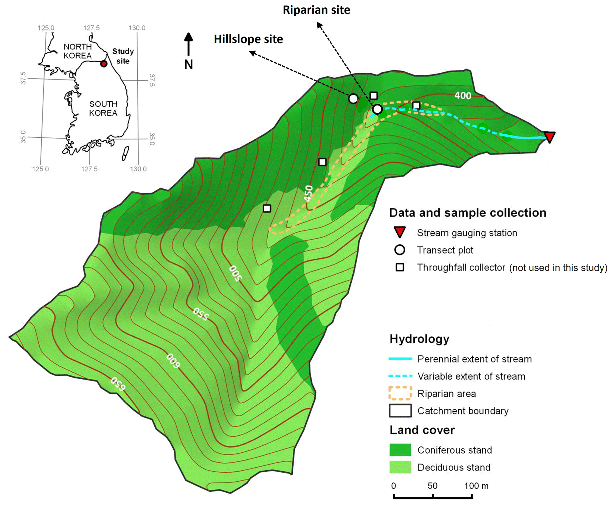
Figure 1 Location and detailed map of the test catchment and sampling setup. Discharge was measured at a V-notch weir installed at the outlet of the catchment (red triangle).

This study explores the value of experimentally derived contributions to streamflow to identify the increase in the accuracy of simulated streamflow components at the catchment scale. We use a modified version of the process-oriented HBV model and Monte-Carlo-based parameter estimation framework to (1) obtain acceptable simulations of total streamflow at the catchment outlet and (2) incorporate experimentally derived information on the contributions of water originating from the hillslope, the riparian zone, and from groundwater to total streamflow into model parameter estimation. By iteratively adding this information to the parameter estimation, we can quantify the impact of the additional data on parameter identifiability and on the uncertainty in discharge simulations during variable flow conditions. We apply our approach at a well-instrumented test site in the monsoonal mountainous north of South Korea during two consecutive seasons.

2 Experimental work and hydrograph separation

2.1 Test catchment

Our test catchment is located in a mountainous area in the northeast of South Korea (Fig. 1) in the Gangwon province (38.2051^∘ N, 128.1816^∘ E). The forested headwater catchment has an area of ∼ 16 ha, with elevations ranging from 368 to 682 $\mathrm{m}\mathrm{a}.\mathrm{s}.\mathrm{l}.$ (above sea level) and a mean slope of 24^∘ (Lee et al., 2016). The headwater catchment has only a narrow riparian zone around the upper part of the stream that comprises approx. 3 % of the catchment area. The bedrock consists of low-permeability quartzofeldspathic orthogneiss. Soils are mostly dystric Cambisols, with a loamy texture and an average thickness of 0.6 m. On the hillslopes, the soil is underlain by a very hard and compact layer of hardpan-like features. A deciduous stand, resulting from natural regeneration after harvest in the 1970s, dominates at elevations above 450 m (61 % of the entire area), whereas, at lower elevations, a coniferous stand prevails that was planted after the harvest at the same time (39 % of the entire area). Precipitation data in daily resolution from a weather station of the Korea Meteorological Administration (station no. 594, located approx. 3 km northeast of the study site in South Korea; https://www.kma.go.kr, last access: 14 March 2023) were obtained for the years 2013 and 2014. In addition, monthly precipitation data from this station were available for the period 1997–2012. South Korea experiences the East Asian summer monsoon during the months of June, July, and August (JJA). Mean annual precipitation was 1273 mm (1997–2014), with, on average, 60 % occurring from June through August. In 2013, the annual precipitation was 1313 mm (897 mm in JJA), whereas 2014 was much drier, with an annual precipitation of 699 mm (364 mm in JJA). During the monsoon season studied in 2013, the stream surfaced 65 m upstream of the catchment outlet at low-flow conditions. During the main monsoon period in 2013, however, the stream extended 226 m upstream of the outlet to the location of the study hillslope transect (Fig. 1).

2.2 Discharge measurements

Discharge was measured at the outlet of the catchment during 2013 and 2014. The water stage was recorded at a V-notch weir every 5 min from 1 June to 31 August 2013 and from 1 June to 16 August 2014, using a pressure transducer (Levelogger Gold M10; Solinst Canada Ltd., Georgetown, ON, Canada) that was barometrically compensated with a barometric pressure transducer (Barologger Gold M1.5, Solinst Canada Ltd., Georgetown, ON, Canada). Discharge was calculated from stage measurements by applying a stage–discharge relationship that was developed based on the procedures outlined in WMO (2010).

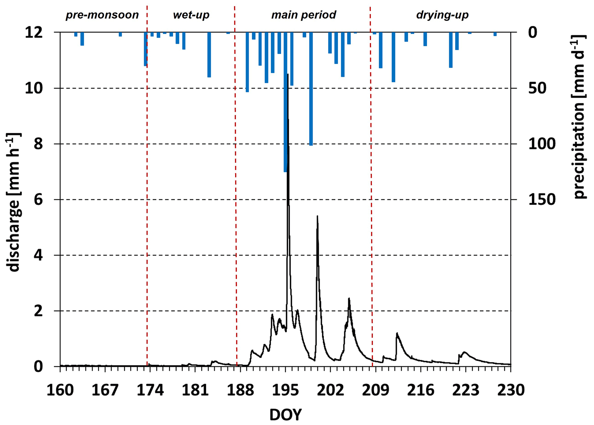
Figure 2 Daily precipitation rates and discharge time series for the monsoon season in 2013 (9 June to 18 August; i.e., day of year, DOY, 160–230). The monsoon season was separated into four periods based on the precipitation and hydrological response.

Figure 2 shows the daily precipitation rates and the discharge time series for the period 9 June to 18 August 2013 (corresponds to day of year, DOY, 160–230). This is the period for which the tracer hydrological work was performed. The monsoon season was separated into four periods based on the precipitation and hydrological response of the headwater stream. The pre-monsoon season (DOY 160–173) corresponded to baseflow conditions (49 mm of precipitation). The wet-up period (DOY 174–187) exhibited some larger rainfall events (79 mm of precipitation) that induced only a small response in discharge. The main period (DOY 188–208) was characterized by frequent large rainfall events (564 mm total precipitation), with an increase in discharge by more than 2 orders of magnitude. During the drying-up period (DOY 209–230), events became infrequent again (150 mm), and discharge quickly receded.

2.3 Water sampling and chemical analyses

The sampling of different water sources was performed between early June and mid-August 2013. The goal was to monitor the dynamics of solute concentrations in streamflow before and during the monsoon season and to characterize the chemistry of soil water from different hillslope positions. Streamflow at the catchment outlet was sampled at least every 2 d (grab samples). During and following major rainfall events, the sampling frequency was increased to several samples per day (grab samples and automated sampling using a 6712 Portable Sampler; Teledyne ISCO, Inc., Lincoln, NE, USA).

Soil water was sampled every 2  d at two different hillslope positions (i.e., on the hillslope in a mid-slope position and in the riparian zone). These two positions formed a transect approx. 200 m upstream of the catchment outlet (Fig. 1). Soil water was extracted using suction lysimeters, installed at 20, 30, and 40 cm depth below the surface. Chemical analyses showed that soil water chemistry was very similar among the three depths; therefore, only values averaged across the three depths were used in this study to represent soil water from the two hillslope positions. Water samples were stored in polypropylene test tubes at 4 ^∘C in the dark until analyses. For more detailed information on instrumentation and methodology please refer to Payeur-Poirier (2018).

The electrical conductivity (EC) of streamflow samples and of collected soil water was measured at the time of sample collection using a portable EC meter (WTW Cond 340i; Xylem Analytics, Weilheim, Germany). Major anions and cations were also determined in the water samples, but here we only report the concentrations of magnesium (Mg). Magnesium was measured by inductively coupled plasma optical emission spectrometry (Optima 3200 XL; PerkinElmer LAS GmbH, Rodgau, Germany), with a detection limit of 10 µg L⁻¹.

2.4 Deriving end-member contributions to streamflow

2.4.1 The hydrograph separation procedure

The procedure of hydrograph separation has the goal to separate the streamflow into its spatial or temporal components. The general procedure of hydrograph separation relies on several assumptions, namely that (1) streamflow can be described as a linear mixture of the so-called end-members, i.e., the contributing components, (2) the end-members have characteristic and differing tracer concentrations, i.e., typical signatures, (3) end-member concentrations are time-invariant, and (4) tracers behave conservatively (Hooper et al., 1990). Any change in tracer concentration in streamflow, i.e., the mixture of components, is only due to a change in the fractional contribution of the end-members to discharge. Pairs of tracers can be explored using bivariate plots, where the concentrations of two tracers in the end-members and streamflow are plotted against each other. If streamflow can be well described by a mixture of the three selected end-members, then streamflow concentrations will fall within the bounds of the triangle that is created by the tracer concentrations of the three end-members. Mixing ratios between the three selected end-members were calculated using mass balances for water and the two tracers, as follows:

$$\begin{array}{}\text{(1)}& \begin{array}{rl}& \mathrm{1}=f_{\mathrm{1}}+f_{\mathrm{2}}+f_{\mathrm{3}}\\ & c_{\mathrm{s}\mathrm{1}}=f_{\mathrm{1}}{c}_{\mathrm{11}}+f_{\mathrm{2}}{c}_{\mathrm{21}}+f_{\mathrm{3}}{c}_{\mathrm{31}}\\ & c_{\mathrm{s}\mathrm{2}}=f_{\mathrm{1}}{c}_{\mathrm{12}}+f_{\mathrm{2}}{c}_{\mathrm{22}}+f_{\mathrm{3}}{c}_{\mathrm{32}},\end{array}\end{array}$$

where c_sj means the concentration of tracer j in stream water, c_ij is the concentration of tracer j in end-member i, and f_i is fractional contribution of end-member i to streamflow. By rearranging these three equations, the three unknowns f₁, f₂, and f₃ can be determined.

2.4.2 Tracer time series in streamflow

For this study, EC and Mg were used as tracers. During the pre-monsoon and the wet-up periods, tracer values in streamflow remained relatively stable (Fig. 3). With the onset of the main period, however, tracer values decreased markedly. Towards the end of the drying-up period, EC values and Mg concentrations started to increase again.

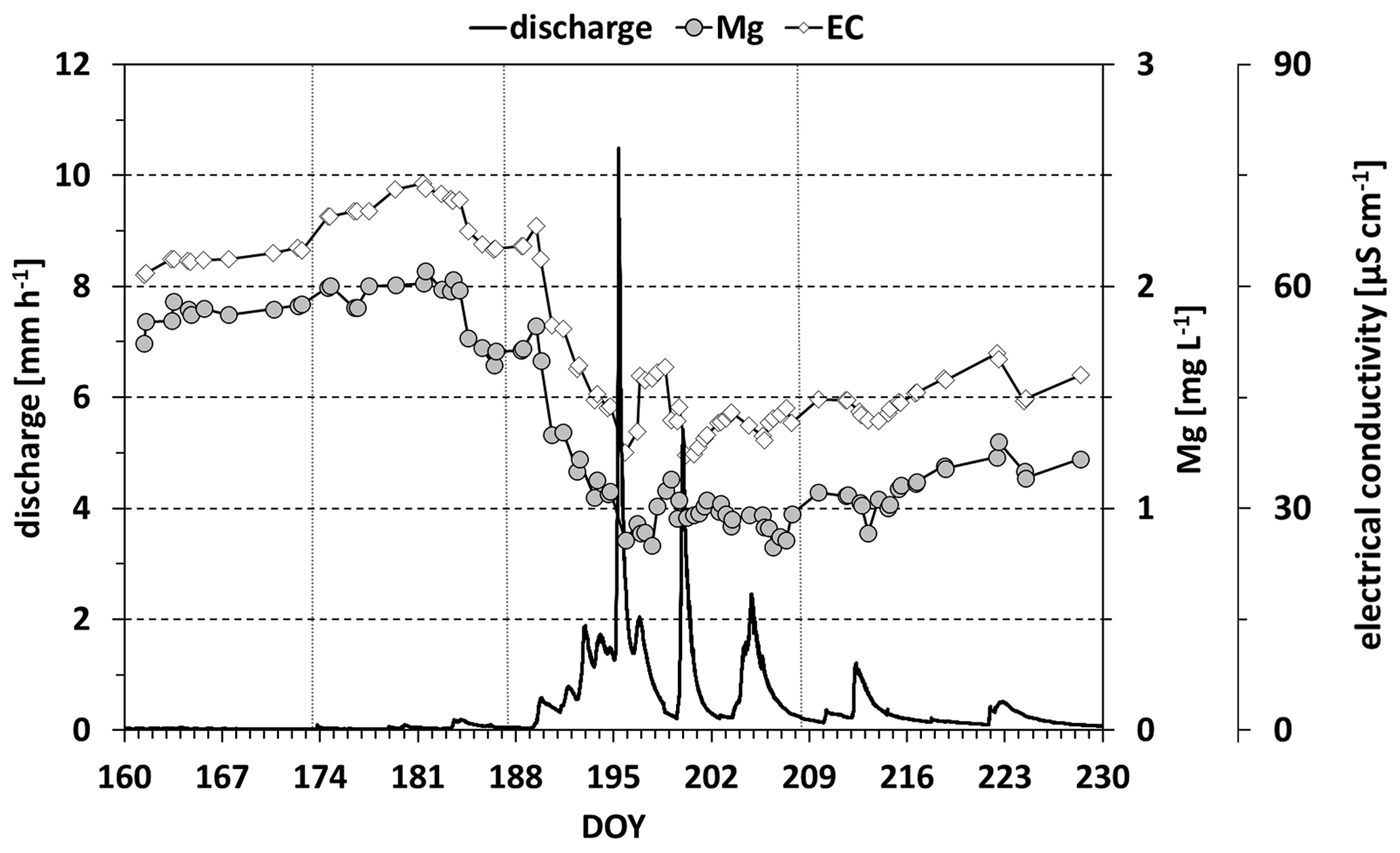
Figure 3 Time series of discharge and of electrical conductivity and magnesium in streamflow. Vertical dashed gray lines separate the four monsoon periods (see also Fig. 2).

Figure 4 Time series of electrical conductivity (a) and magnesium (b) in streamflow and in the end-members' hillslope soil water (soil_hill) and riparian-zone soil water (soil_rip). For the groundwater end-member, the mean of baseflow concentrations during the pre-monsoon period (DOY 160–173) is shown, and the standard deviation (n=11) is a gray band. Vertical dashed gray lines separate the four monsoon periods (see also Fig. 2). The dashed red line signifies the onset of the main period of the monsoon.

2.4.3 Characterizing the tracer signature of the end-members

We defined three end-members (i.e., three water sources potentially contributing to streamflow), namely hillslope soil water, riparian-zone soil water, and groundwater. During the pre-monsoon season, i.e., baseflow conditions, we assumed groundwater to be the only component contributing to streamflow. Since we did not sample groundwater directly, we used the average of the EC values and Mg concentrations measured in streamflow during the pre-monsoon period (DOY 160–173) as the tracer signature of the groundwater end-member. As overland flow was not observed during the fieldwork in 2013, and also direct channel interception was assumed to be negligible in this headwater catchment, we did not consider throughfall to directly contribute to streamflow and therefore did not include it in the hydrograph separation. Hillslope soil water and riparian-zone soil water, sampled as described above, were assumed to contribute via subsurface flow pathways to streamflow.

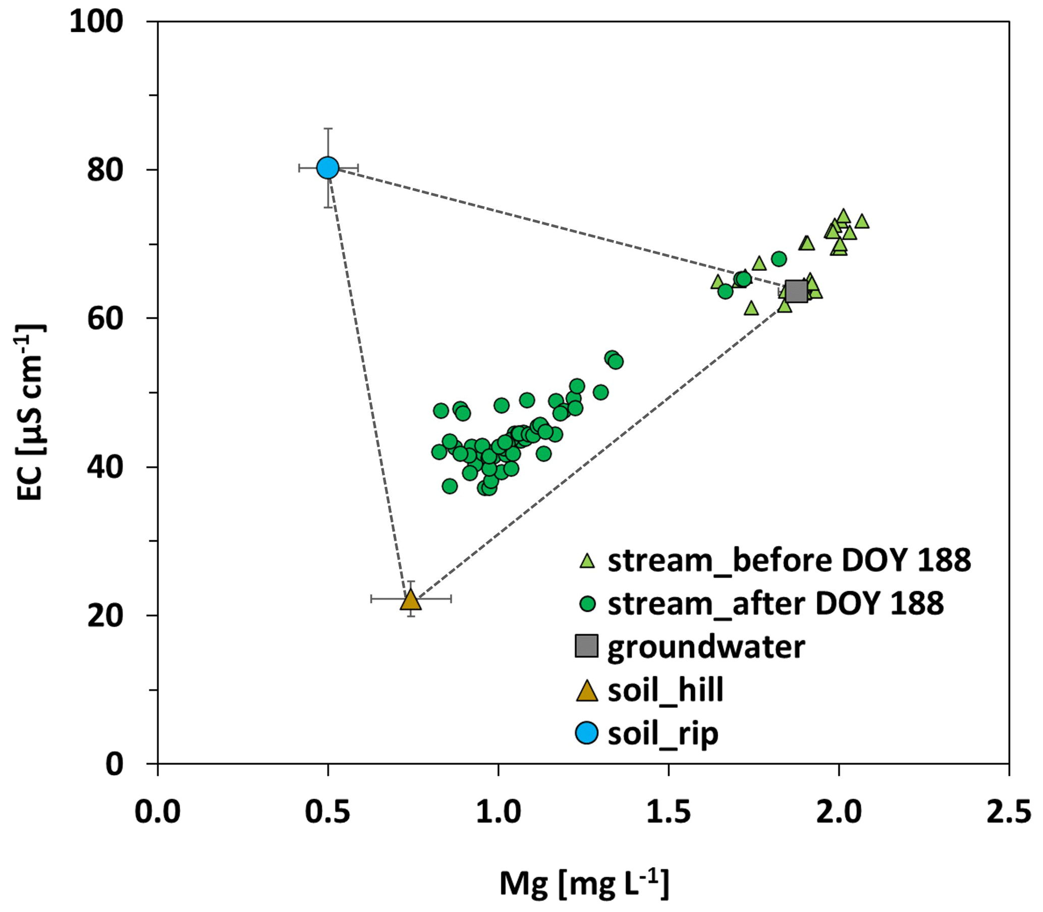
Figure 5 Mixing diagram showing streamflow tracer values for EC and Mg, separated in the period before and after DOY 188 (i.e., onset of the main period), and end-member tracer signatures, including standard deviations (calculated for DOY 188–230).

Hillslope soil water and riparian-zone soil water showed strongly varying tracer values during the pre-monsoon and wet-up periods, i.e., before the onset of the main period, thereby violating the assumption (3) for hydrograph separation listed above (Fig. 4). From DOY 188 on, however, EC values and Mg concentrations remained fairly stable in hillslope soil water (coefficients of variation 11 % and 16 %, respectively) and riparian-zone soil water (coefficients of variation 7 % and 17 %, respectively). Therefore, mean end-member tracer signatures were only calculated for the period DOY 188–230, and the three-component hydrograph separation was only performed for this period, i.e., for the main period and the drying-up period. Based on EC values and Mg concentrations in the stream (Fig. 4) and also general stream water chemistry, we concluded that, from DOY 160 to DOY 187, i.e., also during the wet-up period, streamflow was primarily composed of groundwater. In contrast, streamflow tracer values during the main and drying-up periods could well be described by a linear combination of the three selected components (Fig. 5).

2.4.4 A switch in end-member contributions during the main monsoon period

The hydrograph separation results indicated that, during the main period and the drying-up period, the groundwater contribution decreased considerably, and the signatures of hillslope soil water and riparian-zone soil water became discernible in streamflow, suggesting a substantial contribution to streamflow from the hillsides of the catchment.

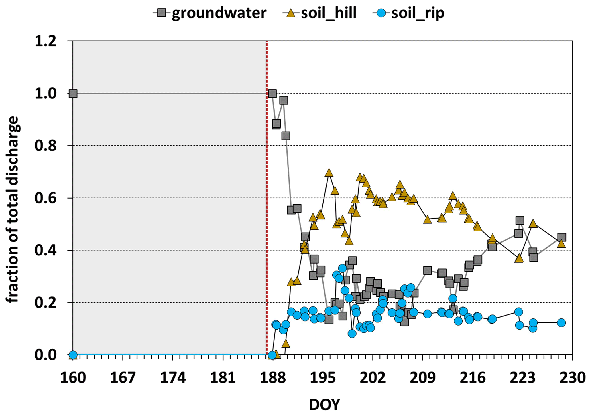
Figure 6 Contributions of the three selected end-members to total discharge for the period DOY 188–230. The dashed red line indicates the onset of the main period of the monsoon. Prior to DOY 188, streamflow was primarily composed of groundwater.

The contribution of groundwater to streamflow dropped from 100 % to values between 20 % and 40 % (mean 34 %) during the main and drying-up periods (Fig. 6). The contribution from riparian-zone soil water varied mostly between 10 % and 21 % (mean 16 %), whereas hillslope soil water contributed between 40 % and 60 % (mean 50 %). This indicates that hydrological connectivity between the hillslopes and the stream was established, and the chemical composition of streamflow was dominated by the hillslope soil water signatures for the main and drying-up periods. This observation is in contrast to other studies that have emphasized the dominant role of the riparian zone in controlling the chemistry of the subsurface flow that enters the stream (Klaus and Jackson, 2018; Ledesma et al., 2018; Bishop et al., 2004; Cirmo and McDonnell, 1997). The specific topography of our test catchment, with steep hillslopes and narrow riparian zones in combination with heavy rainfall events during the intense phase of the monsoon season, results in hillslope-generated subsurface storm flow passing through the riparian zone without undergoing mixing processes. Therefore, the hillslope soil water signature can be detected in streamflow. Most likely, this direct hillslope soil water contribution to streamflow will subside once the headwater catchment drains and the discharge returns to baseflow conditions.

Table 1 Parameters of the modified HBV model, description, units, and boundaries for parameter estimation (see below) and the model performances and simulated streamflow components for the two delineated monsoon periods (see Sect. 2) when confining the initial parameter sample by discharge only and by discharge and tracer-based contributions to streamflow for the calibration in 2013 and the validation in 2014.

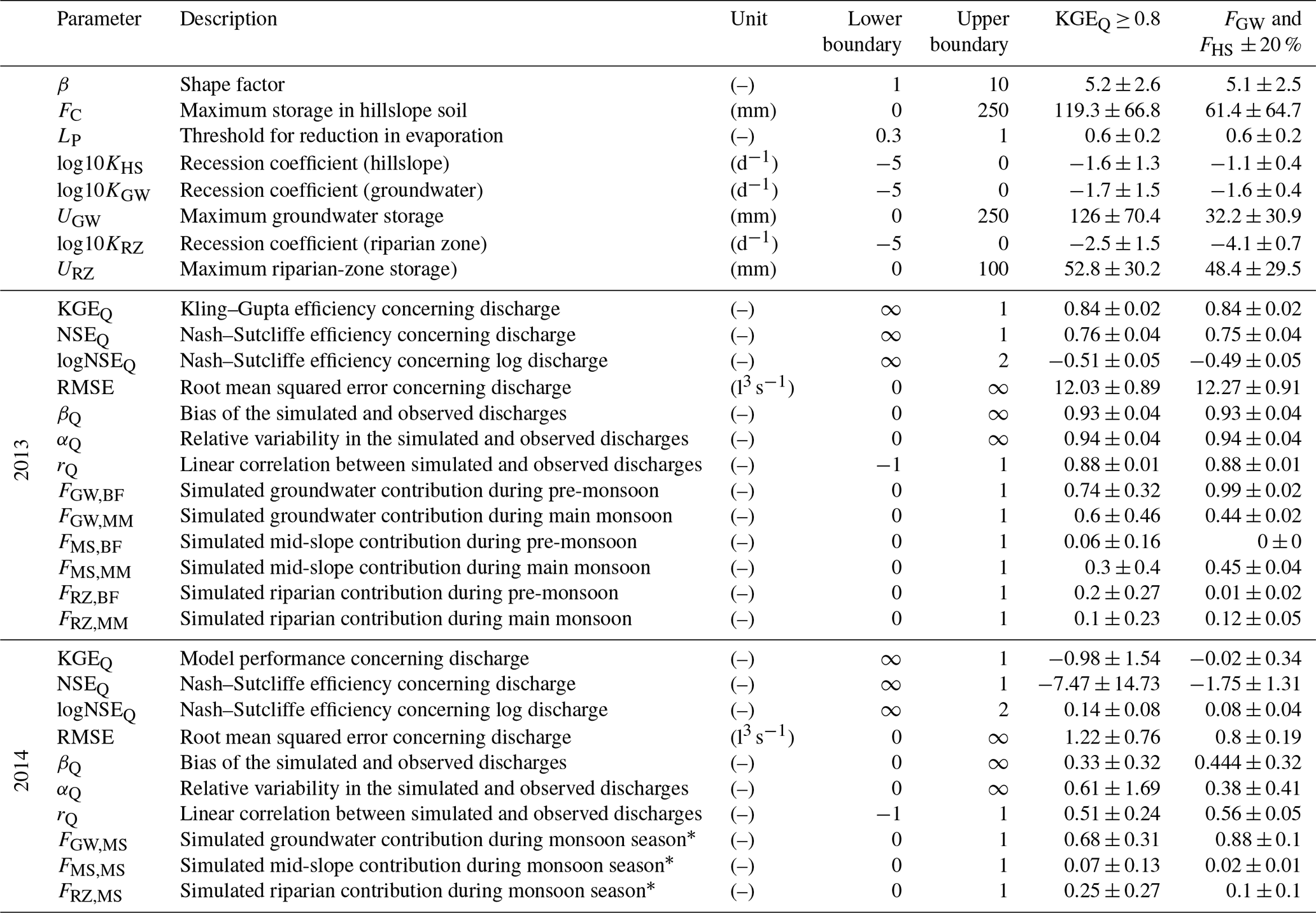
^∗ From 1 April 2014 to 30 September 2014.

3 Methods

We used a process-based, lumped model to simulate the storage and flow dynamics of the hillslope, the riparian zone, and the groundwater for different periods of the 2013 monsoon season by separate subroutines. We used a Monte Carlo approach to create 2×10⁶ simulation time series, which we iteratively confined using the performance criteria of discharge and the mixing ratios estimated by tracer-based three-component hydrograph separation (Table 1). At each step, we quantify the identifiability of model parameters to learn about the usefulness of the discharge observations and hydrograph separation results considered in the confinement procedure. We finally compare the uncertainty in the simulated streamflow components, with and without using the hydrograph separation results, and, using independent discharge observations of the 2014 monsoon season, quantify how much the inclusion of experimentally derived streamflow components can reduce prediction uncertainty.

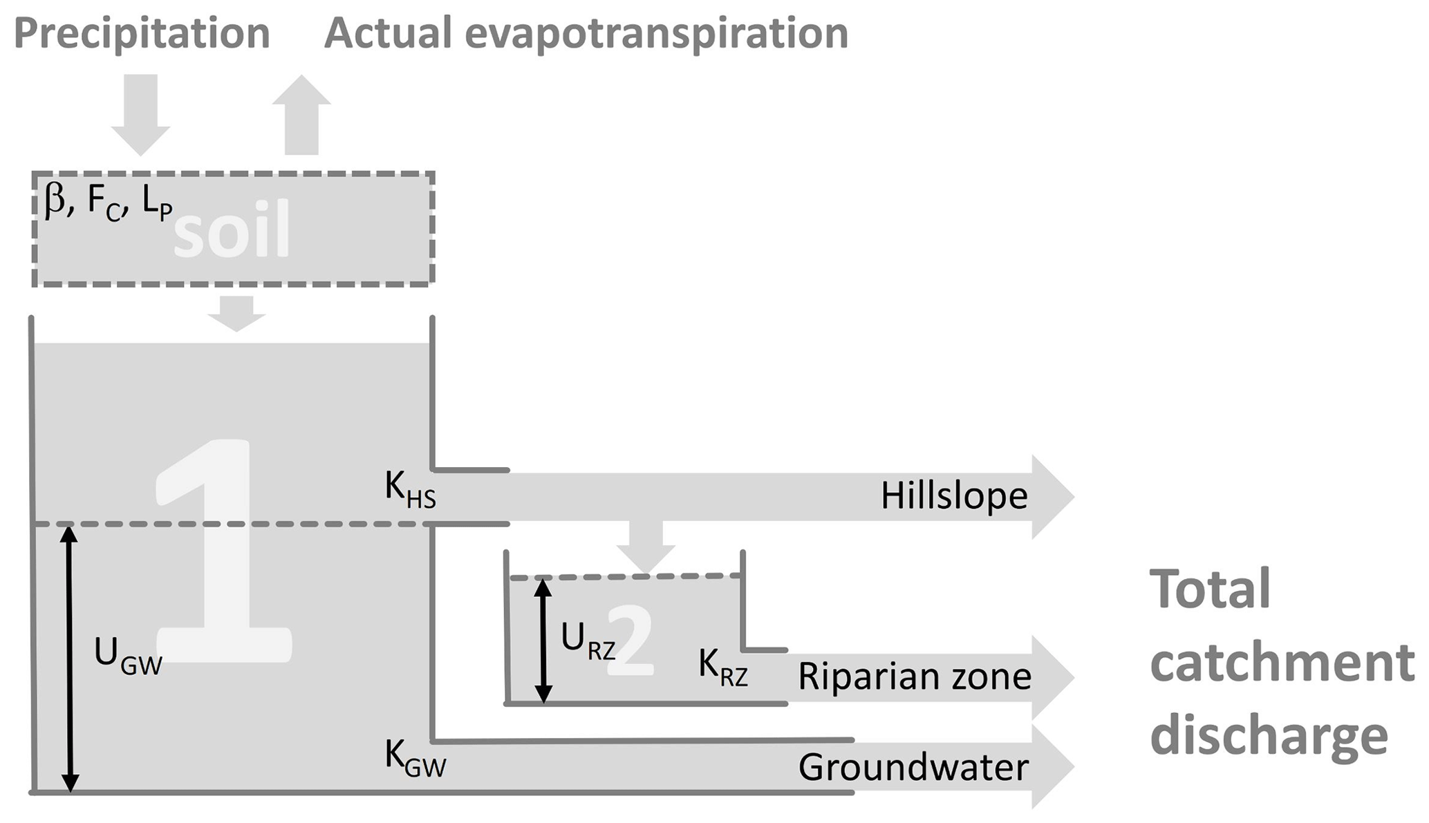
Figure 7 Structure of the modified HBV model. The three components of hillslope, riparian zone, and groundwater sum up to the total catchment discharge.

3.1 The model

We use a modified version of the HBV model (Beck et al., 2010; Seibert and Vis, 2012). The model was modified to include the riparian zone (similar to Seibert et al., 2003) and simplified by removing the snow routine and considering only two reservoirs that simulate the contributions of the hillslope, the riparian zone, and groundwater to total discharge with eight model parameters (Fig. 7; Table 1). The soil storage receives all precipitation (mm d⁻¹) and calculates actual evapotranspiration (mm d⁻¹) from potential evaporation (mm d⁻¹; Penman–Wendling approach; DVWK, 1996; Wendling et al., 1991) by multiplication with an evaporation factor f_Evap (–; 0≤ f_Evaple1), as follows:

$$\begin{array}{}\text{(2)}& f_{\text{Evap}}\left(t\right)={\displaystyle \frac{V_{\mathrm{S}}\left(t\right)}{F_{\mathrm{C}}\cdot L_{\mathrm{P}}}},\end{array}$$

with V_S (mm) as the soil storage at time t, F_C (mm) as the field capacity, and L_P (–) as an evaporation shape factor. A wetness factor f_Wet derived from soil saturation and a shape factor β (–) determines the fraction of precipitation that percolates through the soil, as follows:

$$\begin{array}{}\text{(3)}& f_{\text{Wet}}\left(t\right)={\left({\displaystyle \frac{V_{\mathrm{S}}\left(t\right)}{F_{\mathrm{C}}}}\right)}^{\mathit{\beta }}.\end{array}$$

The remaining part of precipitation (1−f_Wet(t)) is added to the soil storage. Soil percolation is added to the water stored in reservoir one, V₁(t) (mm), which is drained by groundwater discharge Q_GW (mm d⁻¹) and hillslope discharge (sometimes referred to as subsurface storm flow or interflow) Q_HS (mm d⁻¹) when a maximum groundwater storage U_GW (mm) is exceeded. This model process represents conceptually the impact of rising groundwater levels on lateral transmissivities that allow fast saturated flow down the hillslope towards the riparian zone.

$$\begin{array}{}\text{(4)}& {\displaystyle }{Q}_{\text{GW}}\left(t\right)={\displaystyle \frac{V_{\mathrm{1}}\left(t\right)}{K_{\text{GW}}}}\text{(5)}& {\displaystyle }{Q}_{\text{HS}}\left(t\right)=\left\{\begin{array}{ll}\frac{V_{\mathrm{1}}\left(t\right)-U_{\text{GW}}}{K_{\text{HS}}}& \text{if }{V}_{\mathrm{1}}\left(t\right)\ge U_{\text{GW}}\\ \mathrm{0}& \text{if }{V}_{\mathrm{1}}\left(t\right)<U_{\text{GW}}\end{array}\right.,\end{array}$$

where K_GW (d) and K_HS (d) are the storage constant of the groundwater and the hillslope, respectively, and U_GW (mm) is the maximum groundwater storage. Hillslope discharge is fed into reservoir two, which represents the riparian zone until riparian-zone storage V₂(t) exceeds it maximum capacity U_RZ (mm). Discharge of the riparian is therefore defined as follows:

$$\begin{array}{}\text{(6)}& Q_{\text{RZ}}\left(t\right)=\left\{\begin{array}{ll}\frac{V_{\mathrm{2}}\left(t\right)}{K_{\text{RZ}}}& \text{if }{V}_{\mathrm{2}}\left(t\right)<U_{\text{RZ}}\\ \frac{U_{\text{RZ}}}{K_{\text{RZ}}}& \text{if }{V}_{\mathrm{2}}\left(t\right)=U_{\text{RZ}}\end{array}\right..\end{array}$$

Catchment discharge is obtained by summarizing over Q_GW, Q_HS, and Q_RZ at each time t and rescaling them (to m³ s⁻¹) using the catchment area (16 ha). Rescaling the catchment discharge for each time step t, we can express each streamflow component in percent. Similar to preceding work that compared simulated and tracer-derived streamflow contributions (Robson et al., 1991, 1992), we can now compare the model's simulations to the results of the streamflow separation analysis (Sect. 2).

The model operates at a daily temporal resolution to simulate the monsoon seasons of 2013 and 2014 after a warm-up period of 3.5 years. Precipitation data from a nearby meteorological station of the Korean Meteorological Administration (see Sect. 2) and from a global product (Global Land Data Assimilation System (GLDAS; Rodell et al., 2004), corrected with the observations from the local weather station, were used to complete the missing observations before the 2013 monsoon season and between the two monsoon seasons. Since reliable hydrograph separation results are only available for the 2013 monsoon season, we use this year for model calibration, whereas the monsoon season of 2014, for which only discharge observations are available, was used for the validation of the model.

3.2 Stepwise parameter estimation and quantification of parameter identifiability

Similar to the generalized likelihood uncertainty estimation (GLUE) framework (Beven and Binley, 1992), we use a “soft rules” approach to estimate model parameters and their identifiability that allows the consideration of different types of observations (Hartmann et al., 2017; Sarrazin et al., 2018; Chang et al., 2020). We apply a Monte Carlo parameter sampling to obtain 2×10⁶ model realizations derived by uniform sampling of model parameters within their predefined ranges (Table 1). For each run, we calculate the model performance concerning observed catchment discharge with the Kling–Gupta efficiency KGE_Q (Gupta et al., 2009) that indicates flawless simulations with a value of 1 and simulations worse than the simple average of the observations with a value of −0.41 (Knoben et al., 2019) and the deviation of observed and simulation contributions of groundwater F_GW (%) and mid-slope discharge F_HS (%) over the two monsoon sub-periods, for which stable end-member estimates were available (pre-monsoon and wet-up and main monsoon and drying-up periods, as defined in Sect. 2.4). In a three-step procedure, we remove those model realizations that perform poorly against discharge or streamflow contribution observations with rather soft thresholds for F_GW and F_HS to account for the comparably large uncertainties in multicomponent streamflow separation (Genereux, 1998) and simplifications of our simulation model (see Sect. 3.1).

1. We reduce the sample by discarding all simulations that perform badly in terms of observed total streamflow by removing all simulations with KGE_Q < 0.8.

2. We further reduce the sample by removing all simulations whose F_HS show more than 10 % deviation from the hydrograph separation estimates. The relatively large value of 10 % was chosen because of the uncertainty in the end-members (as described in Sect. 2.4) and previous hydrograph separations (Genereux, 1998). Its final value of 10 %, found with a trial-and-error procedure, accounts also for the uncertainties arising from simplifications in our simulation model.

3. We further reduce the sample by removing all simulations whose F_GW show more than 20 % deviation from the hydrograph separation estimates. Since the contributions of the hillslope, groundwater, and the riparian zone sum up to 100 %, riparian-zone contributions are implicitly considered in this last step.

To estimate changes in the identifiability of the model parameters through adding more and more information along the three-parameter confinement steps, we quantify the strength of reduction in the initial sample of 2×10⁶ and the change in the distribution of each model parameter at each individual step. If discharge observations or one of the hydrograph separation streamflow components provides information to better estimate model parameters, a strong decrease in the initial sample and a substantial change in a large number of model parameters should be found. To analyze the sensitivity of our results to the selection of the two thresholds (KGE_Q < 0.8, and F_HS and F_GW ± 10 %), we relax their values and repeat the analysis two times (once with KGE_Q < 0.5 (and F_HS and F_GW ± 10 %) and once with F_HS and F_GW ± 20 % (and KGE_Q < 0.8)).

3.3 Quantification of uncertainty in simulated model internal fluxes and discharge

We quantify the simulation uncertainty in discharge by the mean and standard deviations of KGE_Q, obtained by using only observed discharge or both observed discharge and the hydrograph separation results for parameter confinement for the calibration period in 2013 and the validation period in 2014. Similarly, to quantify the simulation uncertainty in the simulated internal fluxes (hillslope discharge, groundwater discharge, and riparian-zone discharge), we compare their simulated means and standard deviations that were obtained (by using only observed discharge or by both observed discharge and the hydrograph separation results for parameter confinement) with the hydrograph separation derived from streamflow components during the two time periods of the 2013 sampling period. We do the same for the 2014 monsoon season, but since there are no reliable hydrograph separation results available for this year, we only analyze the simulated mean and standard deviation of the simulated streamflow contributions for both calibrations. If the hydrograph separation derived from streamflow components provides new information for parameter estimation, then it will result in a reduction in the uncertainty in the simulated fluxes and discharges in both years and an increase in the KGE_Q of the 2014 predictions should be found. In order to better interpret model performances and simulation uncertainties, we calculate additional performance metrics (equations provided in the Supplement), including the Nash–Sutcliffe efficiencies, the logarithmic Nash–Sutcliffe efficiency, the root mean squared error, and the individual components of the Kling–Gupta efficiency (bias, variability, and correlation).

4 Results

4.1 Stepwise parameter estimation and quantification of parameter identifiability

When iteratively applying the three rules for parameter confinement, we observe a substantial decrease in the initial sample of 2×10⁶ parameter sets (Fig. 8). Extracting only those with KGE_Q ≥ 0.8 reduces the sample to less than 10 % (137 137 parameter sets left). Adding the observed streamflow components to the calibration procedure results in a further reduction in the sample. Discarding all parameter sets that deviate more than 10 % from the observed hillslope contributions results in 2786 remaining parameter sets and in 56 parameter sets when the groundwater contributions (and, implicitly, the riparian-zone contributions) are finally added. Despite being only average values over the two sub-periods of the 2013 sampling period, the incorporation of the hydrograph separation derived from streamflow contributions results in a reduction by more than 3 orders of magnitude, while the discharge observations, although using a high value of 0.8 of the KGE_Q criterion, only reduced the sample by slightly less than 1 order of magnitude.

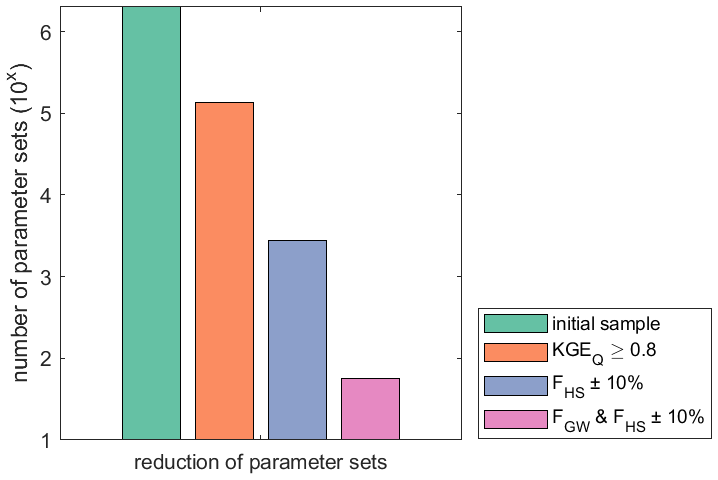
Figure 8 Iterative reduction in the initial sample of 200 000 parameter sets using the KGE_Q and hydrograph separation derived from streamflow contributions for the individual years 2013 and 2014, in addition to both years together.

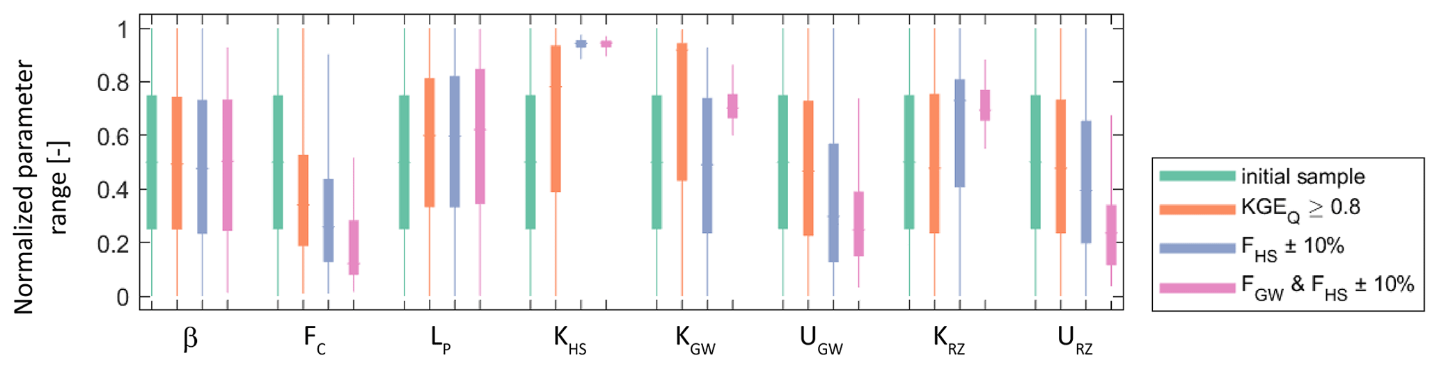
Figure 9 Initial parameter distribution and their modification along the three parameter estimation steps for the individual years 2013 and 2014, in addition to both years together. Boxes indicate the range between the 25th and 75th percentiles, and the lower and upper whiskers show the 5th and 95th percentiles, respectively.

The influence of the parameter confinement procedure using observed discharge and streamflow components is also visible through the changes in the distribution of each of the parameters occurring at each of the confinement steps (Fig. 9). When only discharge is considered in the first step of the confinements (KGE_Q ≥ 0.8), then some model parameter distributions shift away from the mean of the normalized range (e.g., L_P, K_HS, or K_GW), but only one of them, F_C, shows a confinement of its 25th and 75th percentile, which indicates a reduction in the uncertainty. When the sample is further confined by the observed streamflow contributions of the hillslope, a few more parameters shift away from the mean (e.g., U_GW and U_RZ), but two more parameters, K_HS and K_RZ, show confined uncertainties. When finally adding the groundwater contributions (and, implicitly, the riparian-zone contributions), almost all model parameters show a clear shift in their distributions away from the mean for most of them going along with a reduced uncertainty indicated by the narrowing 25th and 75th percentiles. We find the same results when calculating the mean and standard deviations of the model parameters for the confinement by discharge only and the confinement by discharge and the experimentally derived (i.e., tracer-based) contributions to streamflow (Table 1).

Changing the thresholds towards more relaxed rules, once with KGE_Q < 0.5 (and F_HS and F_GW ± 10 %) and once with F_HS and F_GW ± 20 % (and KGE_Q < 0.8), results in a weaker reduction in the initial sample of 2×10⁶ parameter sets, which is most pronounced when relaxing the criteria for the streamflow components towards F_HS and F_GW ± 20 % (Fig. S1 in the Supplement). Consequently, weaker confinements of the parameter distributions are found, whereas K_HS, K_GW, K_RZ, and U_RZ seem to remain identifiable despite relaxing KGE_Q, while F_C, K_HS, K_GW, and U_GW seem to unaffected by the relaxing of F_HS and F_GW (Fig. S2).

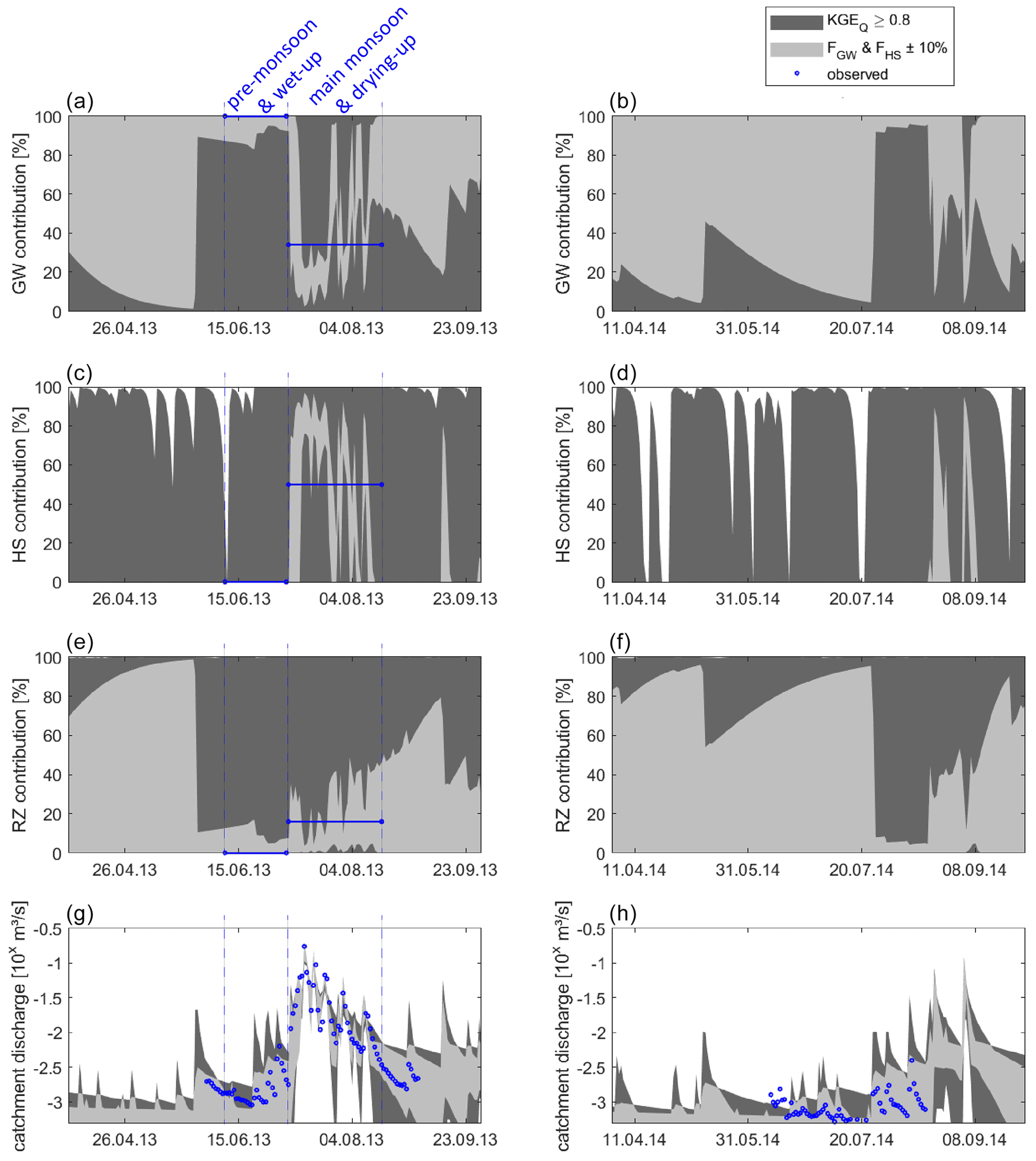
Figure 10 Simulated time series of contributions of groundwater (a, b), subsurface storm flow (c, d), riparian-zone discharge (e, f), and total catchment discharge (g, h; blue points represent discharge observations from the test catchment, and blue lines indicate the experimentally derived contributions to streamflow, averaged over pre-monsoon and main monsoon; see Sect. 2.4) by using discharge (KGE_Q) only and by using F_SSF and F_GW during both years for parameter estimation.

4.2 Quantification of uncertainty in simulated model internal fluxes and discharge

Using only KGE_Q ≥ 0.8 to confine the parameter sample, an average KGE_Q of 0.839, with a relatively low standard deviation of 0.024, is found for the calibration period in 2013 (Table 1), which also results in an acceptable visual agreement between simulations and observations (Fig. 10g). Adding the experimentally derived contributions to streamflow to the parameter confinement results in almost the same mean KGE_Q (0.840), standard deviation (0.023), and visual agreement. However, when looking at the simulated streamflow contributions of the calibration by discharge only, we find that the standard deviations are large compared to the mean simulated contributions of groundwater, hillslope discharge, and riparian-zone discharge across all two monsoon periods (Table 1). Visualizing the entire range of their uncertainties (Fig. 10a, c, and e), we can see that simulated groundwater and riparian-zone contribution could range from 0 % to 100 %. The same is true for the hillslope contributions during wet-up, main monsoon, and drying-up periods. Only during drier periods are hillslope contributions to discharge limited and sometimes drop down to 0 %. Adding the experimentally derived contributions to streamflow to the parameter confinement reduces the simulation uncertainty in all three streamflow components for the two monsoon periods in 2013, as indicated by their strongly reduced standard deviations in Table 1 and by the narrower ranges around the observations of their simulations in Fig. 10a, c, and e. The strong dominance of the groundwater streamflow component during the baseflow and wet-up periods is well represented, as is the onset of hillslope discharge during the main monsoon and the drying-up periods, when the contributions of the riparian zone to streamflow gradually increase. The simulations also indicate that hillslope discharge mostly replaces groundwater in the main monsoon and the drying-up periods, while before and after the monsoons season, streamflow is comprised by an interplay of groundwater and riparian-zone discharge. The comparison of simulations and observations also indicates that strong variations in streamflow components occur even within the monsoon periods, especially during the main monsoon and the drying-up periods (Fig. 10a, c, and e).

During the validation in 2014, a simulated performance of discharge decreases for both calibration steps (Table 1). Using only discharge observations, a very poor simulation quality (KGE_Q = −0.98) is found, with a standard deviation of 1.54, indicating a very high simulation uncertainty. When using both discharge and streamflow components for calibration, a much better performance is found (KGE_Q = 0.02), which is well above the KGE that would be obtained when using just the average observations to predict discharge (−0.41) and which has a much smaller simulation uncertainty indicated by a standard deviation of 0.09, which is confirmed when comparing simulated and observed time series (Fig. 10h). Although there are no observations of the streamflow components available for the validation year 2014, we can still see that the simulation uncertainty in all three components indicated by their standard deviations is generally high over the whole simulation period when only discharge is used for calibration and reduced by more than a third when the stream contributions are considered in the calibration (Table 1). Similar to the calibration year 2013, we see that the interplay between groundwater and the riparian zone is much better defined and that the short but pronounced initiation of hillslope discharge is much better represented when both observed discharge and streamflow components are used for calibrations (Fig. 10b, d, and f).

Considering the other discharge performance metrics, we see that NSE_Q and the individual components of the KGE (β_Q, α_Q, and r_Q) reflect what is already shown by KGE_Q (i.e., a high-simulation performance of discharge for both calibration types for the year 2013). Likewise, RMSE_Q indicates small errors in the range of ∼ 0.012 m³ s⁻¹. Only logNSE_Q deviates from the general impression of acceptable model performance, indicating poor simulation performance of the model for low flows for both calibration types. For 2014, we find that NSE_Q and the individual components of the KGE (β_Q, α_Q, and r_Q) again reflect what is shown by KGE_Q, which is in this case an inferior performance compared to 2013. But logNSE_Q and RMSE_Q indicate a lower simulation error and a better low-flow performance for 2014, respectively.

5 Discussion

5.1 Realism of model simulations

We use a simple approach to incorporate streamflow contributions derived from environmental tracers into our simulation approach that compares simulated streamflow contributions and tracer-derived streamflow contributions instead of simulating tracer transport directly. In that way, no additional uncertainty due to additional model parameters was introduced due to additional model parameters to consider transport (Birkel and Soulsby, 2015). Despite its simple structure, the model easily achieves performances of KGE ≥ 0.8 with more than 130 000 parameter sets (out of an initial 2×10⁶; Fig. 7), indicating the adequacy of its structure for simulating the hydrology of our small forested mountainous catchment. Such a good performance could be expected, since similar models, such as the HBV model or similar modifications of the HBV model, already performed well at similar landscapes (Seibert et al., 2003; Uhlenbrook et al., 1999; Chen et al., 2018). Including the experimentally derived contributions to streamflow results in a further substantial reduction in the initial parameter sample to 56 parameter sets and in a slight decrease in overall discharge simulation performance, as indicated by different performance metrics (Table 1). Such a further reduction in the parameter sample is due to the increased difficulty in simulating both discharge and streamflow contributions adequately and simultaneously and was already found in previous studies that investigated the influence of additional information in a GLUE-like approach (Mudarra et al., 2019; Hartmann et al., 2017). Relaxing the thresholds to confine the sample resulted in weaker reductions in the initial parameter sample and parameter distributions that indicate lower parameter identifiability, but the overall results of the stepwise parameter estimation did not change (Figs. S1 and S2).

Likewise, a decrease in the simulation uncertainty concerning discharge, going along with incorporating additional information into parameter estimation, has already been observed (Birkel et al., 2014; Yang et al., 2021; Seibert and McDonnell, 2002). This mostly went along with an increased identifiability of the model parameters and prediction skill, which is also found in this study. Using only discharge for model parametrization, a mean KGE of −0.98 in the validation year of 2014 is found (Table 1). The parameter sets obtained from using both discharge and experimentally derived contributions to streamflow result in a mean KGE of 0.02. Compared to the performances of KGE ≥ 0.8 that we obtained during the calibration in year 2013, this appears to be a strong decrease, but it is substantially better than using the mean of discharge observations for prediction (that would result in KGE = −0.41; Knoben et al., 2019). Also, while the discharge observations in the calibration year 2013 cover the entire stream response to the monsoon season (maximum observed discharge > 0.15 m³ s⁻¹; Fig. 10), the validation time period of 2014 it is much drier than 2013, and it stops before the onset of the late and weak monsoon events in late August that produced increased discharge observations (observed discharges < 0.004 m³ s⁻¹; Fig. 10). For that reason, we consider the evaluation to be more rigorous through the challenge of predicting low flows with a calibration period of 2013 covering the entire variability in streamflow (Nicolle et al., 2014). This is also supported by the RMSE_Q and logNSE_Q values of the discharge predictions that indicate a lower simulation error and a better low-flow performance for 2014, respectively.

5.2 Identification of model parameters and processes

The acceptable multivariate performance of the model in the calibration period and the still-acceptable performance found in the validation period gives us reason to believe that our approach provides interpretable results. Incorporating experimentally derived contributions to streamflow into parameter estimation results in reduced parameter uncertainty for all model parameters, except for β and L_P (which remain the same), compared to the parameter estimation using discharge only (Table 1). The iterative inclusion of observations into the parameter estimation procedure allows the assessment of the usefulness of each type of information. When only discharge is considered, changes in the distributions of parameters L_P, K_HS, or K_GW and F_C occur (Fig. 9), confirming the well-known fact that only four to six model parameters can be identified when calibrating a model with discharge observations only (Ye et al., 1997; Wheater et al., 1986; Jakeman and Hornberger, 1993). When the experimental information of the contributions of the hillslope subsurface flow to streamflow is added, then more parameters change their distributions, indicating that additional information is added to the parameter estimation. We can see that this is most pronounced for K_HS, which controls the discharge dynamics of the hillslope, and U_GW, which indirectly controls hillslope discharge by triggering it after the saturation of the groundwater storage (Fig. 7). Adding the experimentally derived contributions of groundwater (and, implicitly, information about the riparian-zone contributions, as all three together sum up to 1), we see an increase in the identifiability of K_GW, which is indicated by a further narrowing of its 25th and 75th percentile. Most prominently, K_RZ and U_RZ show substantial confinement, indicating that the new information about streamflow contributions added more information about riparian-zone and groundwater dynamics.

Previous work with a model that simulated discharge and solute transport already showed that added information through environmental tracers can be linked to their origin in the hydrological system and respective model parameters (Yang et al., 2021; Hartmann et al., 2017; Birkel et al., 2014). Our results indicate that, even without the explicit inclusion of solute transport in the model, similar linkages between the observations of streamflow contributions and model parameters that control the dynamics of their origin (hillslope, groundwater, or riparian zone) could be found. These relationships are plausible and can be regarded as a validation of the realism of the model structure (McMillan et al., 2012; Capell et al., 2012; Hartmann et al., 2013). By including discharge and observed streamflow components into parameter estimation without adding more complexity to the model, we achieve desirable levels of model parameter identifiability (eight out of nine parameters) and prediction uncertainty (Birkel and Soulsby, 2015). The resulting parameters express the effective properties of our test catchment with a thin soil (F_C = 61.4 mm ± 64.7 mm) and the fast percolation of water towards the hillslope and groundwater storages through a high value of β (5.1 ± 2.5). The value of L_P (0.6 ± 0.2) indicates that plant water uptake through forest cover is efficient, even below the saturation of the soil. The groundwater storage can store more than double the soil, while the riparian-zone storage is about 15 mm smaller (Table 1). With around 0.08 d⁻¹, K_HS indicates fast hillslope dynamics after initiation, while at around 0.025 d⁻¹ and below, K_GW and K_RZ are reacting slowly. The scales of the three parameters are comparable to the parameters identified by Uhlenbrook et al. (1998), who found 0.1–0.35 and 0.02–0.05 d⁻¹ for their simulated interflow and groundwater dynamics, respectively.

5.3 Benefits of including experimentally derived contributions to streamflow for streamflow prediction

The simulated streamflow contributions obtained by discharge during the same period show considerable uncertainty allowing for contributions of groundwater and the riparian zone, from 0 % - 100 %, throughout the entire simulation period of 2013 (Fig. 10a and c), despite the high performance in simulating discharge (Fig. 10g; Table 1). Just for the hillslope contributions, the calibration by discharge only indicates possible contributions <100 % during the baseflow period but shows the same uncertainty as the simulated groundwater and riparian-zone contributions when the pre-monsoon and wet-up monsoon periods begin (Fig. 10e). This strong uncertainty in the three simulated streamflow contributions, despite the high-discharge-simulation performance, is a textbook example of the equifinality problem (Perrin et al., 2001; Beven, 2006) that is known to result in poor prediction performance, as we also found in this study when using discharge for parameter estimation only. With the experimentally derived contributions to streamflow considered in the calibration, the simulated time series of all three contributions (groundwater, hillslope, and riparian zone) become more distinguishable, especially during the main monsoon and the drying-up periods of the 2013 monsoon (Fig. 10a, c, e). We clearly see that the simulated groundwater contribution dominates the discharge in the pre-monsoon and wet-up periods, following the observed contribution of groundwater. At the same time, the riparian-zone contributions confine themselves to their observed values close to 0 %. During the main monsoon and the drying-up periods, the observed contributions of the hillslope are – on average – enveloped by the model simulations, resulting in a substantial decrease in the groundwater contributions.

Strongly different model internal behavior that results in almost the same discharge performance was also observed by Seibert and McDonnell (2002), who showed, with a similar model, that two completely different model setups can produce very similar discharge simulation performance. Among the different types of hard and soft data, they also showed the value of observed streamflow contributions for reducing model parameter uncertainty but only focused on two streamflow components (new water and old water) at peak discharge for six separate rainfall–runoff events (McDonnell et al., 1991). In our study, we distinguish three different streamflow components temporally disaggregated over two periods that resulted in parameter uncertainty reductions that could be attributed to the respective flow and storage processes at their origin (Sect. 5.2). In addition, using the monsoon year of 2014, we can show that the discharge prediction performance of the model increased and simulation uncertainty decreased when the streamflow contributions are considered during parameter estimation (Fig. 10h; Table 1). This is due to the improved representation of the three flow components in the model that indicate, like the monsoon period in 2013, that the model could have overestimated the contribution of the riparian zone and underestimated the contributions of groundwater, and it could have incorrectly predicted the onset and cessation of the hillslope contributions to discharge. Such a decrease in the predictive uncertainty was also revealed in other studies (Son and Sivapalan, 2007; Hartmann et al., 2017), but to our knowledge, it has neither been achieved by using more than two experimentally separated streamflow components, nor without accepting additional uncertainty through the incorporation of transport routines into the model.

6 Conclusions

The value of environmental tracers in improving the realism and prediction skills of hydrological models has been tested and proved in many previous studies. However, few studies were able to include them without adding more complexity to their models due to the conclusion of transport routines. Our study shows that, by directly comparing simulated and experimentally derived streamflow contributions, information derived from environmental tracers can be considered without adding transport routines to our model. Considering the contribution of three streamflow components, namely the hillslope, riparian zone, and groundwater, at two separate periods during a strong change in hydrological boundary conditions, we a provide strong indication that it is worth considering the temporal dynamics of components that express more than just pre-event and event water in the model. Including this information in our stepwise parameter estimation procedure, we obtain increased parameter identifiability and decreased simulation uncertainty in the validation period when compared to using discharge only for calibration. Incorporating the contributions of different components iteratively, we can show that they increase the identifiability of the parameters related to the dynamics of their origin (e.g., the hillslope flow and storage dynamics when hillslope contributions to streamflow are considered). Considering all three observed streamflow components, we can identify all nine model parameters compared to just five parameters when using discharge only for calibration. Consequently, the uncertainty in predicted streamflow in 2014 decreases, along with an increased precision of predicted streamflow components.

Our study adds to the large body of preceding work that provides evidence for the usefulness of incorporating auxiliary data into model calibration. In particular, it shows that the full potential of incorporating streamflow contributions obtained by environmental tracers has not yet been explored. On the one hand, including estimated streamflow contributions from multiple sources (not just event and pre-event water) allows an enhanced improvement of the simulation of model internal processes, especially those that are seldom monitored, such as hillslope contributions through subsurface storm flow (Chifflard et al., 2019). On the other hand, considering the dynamics of those streamflow contributions over time provides a more thorough distinction between realistic and unrealistic parameter combinations. We see that, among the two periods that we considered, the observations for the pre-monsoon and wet-up periods are enveloped well by the simulations. But the temporal resolution of experimentally derived contributions to streamflow during the main monsoon and the drying-up periods seem to be too coarse, as the simulations show much higher temporal variability (while their average seems to follow the observed contributions). Hence, future efforts may involve the monitoring and integration of streamflow components into the model at a higher temporal resolution. Furthermore, by separating the contributions of streamflow components of different origin, our approach might be suitable for the parameterization of hillslope processes in more complex and spatially distributed models at larger scales (Holmes et al., 2022; Stadnyk et al., 2013; Fan et al., 2019).