the Creative Commons Attribution 4.0 License.
the Creative Commons Attribution 4.0 License.
 | 14 Mar 2023
Regionalisation of rainfall depth–duration–frequency curves with different data types in Germany
Winfried Willems
Henrike Stockel
Luisa-Bianca Thiele
Uwe Haberlandt
Rainfall depth–duration–frequency (DDF) curves are required for the design of several water systems and protection works. For the reliable estimation of such curves, long and dense observation networks are necessary, which in practice is seldom the case. Usually observations with different accuracy, temporal resolution and density are present. In this study, we investigate the integration of different observation datasets under different methods for the local and regional estimation of DDF curves in Germany. For this purpose, two competitive DDF procedures for local estimation (Koutsoyiannis et al., 1998; Fischer and Schumann, 2018) and two for regional estimation (kriging theory vs. index based) are implemented and compared. Available station data from the German Weather Service (DWD) for Germany are employed, which includes 5000 daily stations with more than 10 years available, 1261 high-resolution (1 min) recordings with an observation period between 10 and 20 years, and finally 133 high-resolution (1 min) recordings with 60–70 years of observations. The performance of the selected approaches is evaluated by cross-validation, where the local DDFs from the long sub-hourly time series are considered the true reference. The results reveal that the best approach for the estimation of the DDF curves in Germany is by first deriving the local extreme value statistics based on Koutsoyiannis et al.'s (1998) framework and later using the kriging regionalisation of long sub-hourly time series with the short sub-hourly time series acting as an external drift. The integration of the daily stations proved to be useful only for DDF values of a low return period (T[a] < 10 years) but does not introduce any improvement for higher return periods (T[a] ≥ 10 years).
- Article
(11043 KB) - Full-text XML
- BibTeX
- EndNote


Rainfall volumes at varying duration and frequencies are required for the design of water management systems and facilities, like dams or dikes, spillways, flood retention basins or urban drainage systems. These design precipitation volumes are also known as IDF (intensity–duration–frequency) or DDF (depth–duration–frequency) curves, and they are derived from an extreme value analysis (EVA) on observed rainfall. For sampling extreme values, either annual maximum series (AMS) or peak over threshold (POT) can be used; however, for return periods greater than 10 years, there are hardly any differences between the two. Often the AMS is preferred over the POT because the methodology is more direct and easier, whereas the POT method needs a prior assumption on the threshold selection. Afterwards, a theoretical probability distribution (PDF) is fitted to the extreme series of a certain duration, in order to extract design rainfall volumes at a specific frequency (or return periods). Typically, a generalised extreme value (GEV) distribution is fitted for the AMS series and a generalised Pareto for the POT series extracted for a fixed duration level. Rainfall extremes of different durations are strongly related to each other; however, if the parameter fitting is done independently to each duration level, these relations may not be kept (Cannon, 2018). Therefore, generalised concepts as in Koutsoyiannis et al. (1998) and simple scaling (Gupta and Waymire, 1990) or multi-scaling Van de Vyver (2015) approaches are used to smooth the extreme statistics over different duration levels. Finally, since the rainfall observations are mostly point measurements, a regionalisation procedure of the PDF parameters to unobserved locations is performed. Methodologically, a distinction can be made between the two approaches: (a) a direct regionalisation of quantiles, moments or parameters of distribution functions; and (b) a regional estimation of distribution functions for homogeneous regions. Borga et al. (2005) suggest the regionalisation of the parameters instead of the quantiles. For the direct regionalisation of parameters, regressions (Madsen et al., 2009; Smithers and Schulze, 2001), splines (Johnson and Sharma, 2017) or kriging methods (Ceresetti et al., 2012; Kebaili Bargaoui and Chebbi, 2009; Uboldi et al., 2014; Watkins et al., 2005) are applied. On the other hand, the estimation of regional distributions functions based on the index method proposed by Hosking and Wallis (1997) is one of the most used methods in the literature for the regionalisation of design precipitation (Burn, 2014; Durrans and Kirby, 2004; Forestieri et al., 2018; De Salas and Fernández, 2007).
Since the analysis is performed on extreme values, first very long observations are required to ensure a proper fitting of the GEV parameters, particularly of the shape parameter, which is of decisive importance for extremes of high return periods (larger than a 20-year return period). For instance, Koutsoyiannis (2004a, b) showed clearly that short time series (less than 50 years) can choose falsely a shape parameter of zero (Gumbel distribution) and hide the true heavy-tail behaviour of rainfall extremes (also supported by Papalexiou and Koutsoyiannis, 2013 and Papalexiou, 2018). Second, a dense observation network should be available to ensure an adequate estimation of extreme value statistics also at unobserved locations. A less dense network would cause for instance the kriging interpolated values to be less accurate and the spatial features to be more smoothed in space (Berndt et al., 2014). On the other side, index-based regionalisation can provide a more robust estimation at unobserved locations if larger samples (obtained from denser networks) are used (Requena et al., 2019). Third, a high-resolution observation network (with one or five time steps) is also necessary to estimate extremes of short durations (at scales of minutes or hours) for catchments that respond quickly to rainfall events (i.e. urban or mountainous areas prone to flash floods). At the moment, no perfect observation network that fulfils these three criteria is available, however different networks or data types fulfilling two criteria coexist. For example, daily observation networks are typically very dense (every 10 km) and can have up to 100–150 years of observations but do not capture the extremes at sub-hourly durations. Digital tipping bucket or weighting sensors can measure the rainfall at 1 min time steps and can be dense (every 20–25 km), however they are available mostly after 2000 and are hence too short for EVA. Long observations at 1 min time steps from analogous Hellmann or tipping buckets may be available from 1900–1950 only for some countries (i.e. Germany, Belgium) but are not as dense as digital or daily measurements (> 50 km). Alternatively, weather radar or satellite data can provide rainfall fields at 1 or 4 km2 and 5 min time steps but offer short observations (less than 20 years) and suffer from high inaccuracies (Marra et al., 2019).
To optimise the DDF estimation, different data types have been combined; for instance, Madsen et al. (2017) regionalised extremes in Denmark from 1 min observations with daily interpolated values as a covariate, Bara et al. (2009) employed the simple-scale principle to derive DDF curves for sub-daily duration levels (5 min to 3 h) from daily observations in Slovakia, Goudenhoofdt et al. (2017) used station observations (10 min and varying lengths) to correct radar data and estimate the hourly and daily extremes, and Burn (2014) pooled together long and short observations at 5 min time steps to form the DDF curves in Canada. However, care should be taken when combining information from data types that differ in observation length and temporal and spatial scales. Holešovský et al. (2016) separated the historical data into groups when estimating DDF curves for the Czech Republic (long series with 35–40 and short series with 11–15 years of observations) and concluded that the uncertainty at estimating parameters for the short time series is quite high, especially for high return periods. In the index-based regionalisation, regional L-moments are averaged based on the observation length, which may lead to more stable results (Burn, 2014; Requena et al., 2019), however the interpolated index may still suffer from high uncertainties from pooling together short and long time series. This may also be the case when interpolating local GEV parameters with the kriging theory. The regionalisation of the shape parameter may be not representative if short and long observations are pooled together with same importance, thus keeping a fixed shape parameter may help to mitigate this problem. Nevertheless, further investigation should be done to ensure if long observations, as more reliable, should have more importance than the short ones when regionalising extreme value statistics. Regarding the temporal-scale difference, a study from Paixao et al. (2011) performed in Ontario, Canada, concluded that the scaling factors should not be used for downscaling daily extremes to durations less or equal to 1 h. This is because the extremes at such short durations are governed by other rainfall mechanisms than the daily extremes, and hence a low dependency exists between the two extreme groups. Alternative to the scaling principle, disaggregation schemes can be applied to the daily data in order to obtain adequate extremes (with a return period up to 5 years) for sub-hourly durations (Müller and Haberlandt, 2018). On the other hand, because of the spatial-scale inconsistency between weather radar and gauge observations, the weather radar may not be appropriate to estimate directly extremes of short durations (Marra et al., 2019), however they can still be useful to extract sub-daily extremes if used to disaggregate daily observations, as done by Bárdossy and Pegram (2017). More complex disaggregation procedures that take advantage of the radar information by implementing an extensive parameter set as suggested by Lisniak et al. (2013) may also be used to disaggregate daily observation and estimate the extreme values at sub-hourly durations. Nevertheless, to the authors knowledge, there is no study in the literature that investigates if disaggregated daily time series can be useful in regionalising extreme values statistics when high resolution data are present, and when this is so, if they should have the same weights as high-resolution data.
Lastly, due to lack of data, in most of the literature, the combination of any two or alternative data types for EVA is validated on observations that are not dense or long enough (longer than 40–50 years). Therefore, it would be interesting to test different methods for estimation and regionalisation of DDF curves extracted from different data types on a long and dense network. The German Weather Service (DWD) has a relatively dense observations network (every 50 km) of 1 min rainfall data available from 1950 (60–70 years), that enables a proper validation of EVA for return periods up to 100 years. Additionally, denser digital observations (every 20 km) at 1 min time steps (mainly from 2000), very dense (every 10 km) daily observations (10–120 years), and weather radar observations (from 2000) at 1 km2 and 5 min time steps are also available. As multiple data types coexist in Germany, it is important to investigate the suitability of methods and data types for the extraction and regionalisation of extreme statistics while validating only at the long and dense observations. In Germany, studies either use the Koutsoyiannis approach or a multi/simple scaling approach of GEV parameters to generalise the extremes over different durations. To the authors knowledge, there is no comparison of the two approaches in the literature. The Koutsoyiannis approach has been implemented in Germany by Ulrich et al. (2020) but on a shorter available 1 min dataset (up to 14 years), while Fischer and Schumann (2018) have implemented the multi-scale approach only at a long station (∼85 years). Here we investigate which of these methods gives a more accurate and precise estimation of DDF based on the long and 1 min rainfall data. The same is true also for the regionalisation approaches: to the authors knowledge, there is no comparison between kriging and index-based regionalisation. Naturally, it is interesting to see which of the methods is more appropriate when validated on a long and high-resolution network, where the advantages and disadvantages of each method lie when different data types are integrated, and what combination brings the best outcome. For this purpose, we investigate here three competitive regionalisation methods (ordinary kriging, external drift kriging and index-based regionalisation) based on a different combination of data types (long series, short series, disaggregated daily series from weather radar parameterisation), while validating only on the long and high-resolution observations. At the moment, a revision of the current design storm maps in Germany (KOSTRA-DWD) is required in order to use additional data and state-of-the-art methodology. Therefore, an additional aim of this study is to give the basis for the development of the new design of storm maps in Germany (KOSTRA-2023).
The paper is structured as follows: first, the available datasets for extreme value analysis are introduced in Sect. 2; then, the methods selected for investigation of the local and regional estimation are presented respectively in Sect. 3.1 and 3.2; and the performance assessment and validation are explained in Sect. 3.3. The results are given for each objective as: the best local estimation of extremes in Sect. 4.1, the best regionalisation technique in Sect. 4.2.1, and the best data integration in Sect. 4.2.2. Finally, the obtained maps for Germany are discussed in Sect. 4.3, and the conclusions are given in Sect. 5.
2.1 Available data
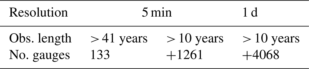
The study area covers Germany and is illustrated in Fig. 1. Three rainfall measuring networks are available from the German Weather Service (DWD): the daily series (DS) – typically Hellman devices recording the rainfall daily, the long series (LS) – mostly tipping bucket analogue sensors (before 2004) measuring rainfall at 1 min time steps with 0.1 mm resolution and 2 % uncertainty, and the most recent short series (SS) – digital sensors (after 2004) measuring rainfall also at 1 min time steps with 0.01 mm resolution. The spatial distribution of these data series is shown in Fig. 1, the observation length is given respectively in Fig. 2, and the number of stations available for each one is given in Table 1. The LS dataset is the most appropriate dataset for extraction and evaluation of extreme rainfall statistics, since on average it includes 65 years of observations (as shown in Fig. 2, dark blue) and measures the rainfall at very fine temporal scales. Nevertheless, this network is sparse in comparison to the other two, and only 133 stations in Germany are available. On the other side, the SS dataset measures the rainfall also at very fine temporal scales and is much denser than the long series (1261 stations excluding the LS locations), however on average it includes only 18 years of observations which is not enough for extreme value analysis. Lastly the DS dataset is much denser (with 4068 stations excluding LS and SS locations) and covers 10 up to 120 years, but the temporal resolution of rainfall is too coarse to be useful for sub-hourly extreme values analysis.
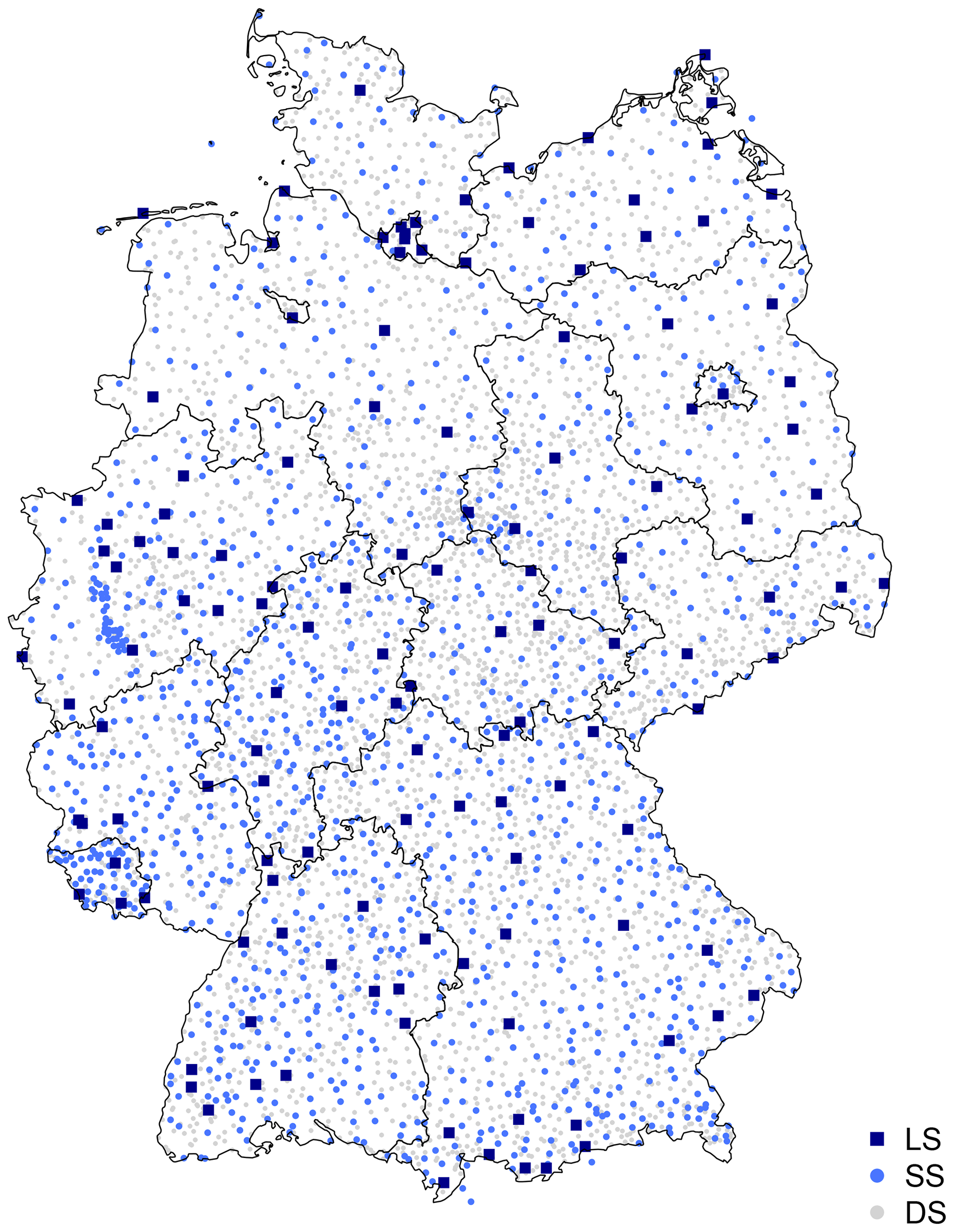
Figure 1Available rainfall data types in Germany categorised in three groups: long series (LS), short series (SS) and daily series (DS). The black lines illustrate the borders of German federal states.
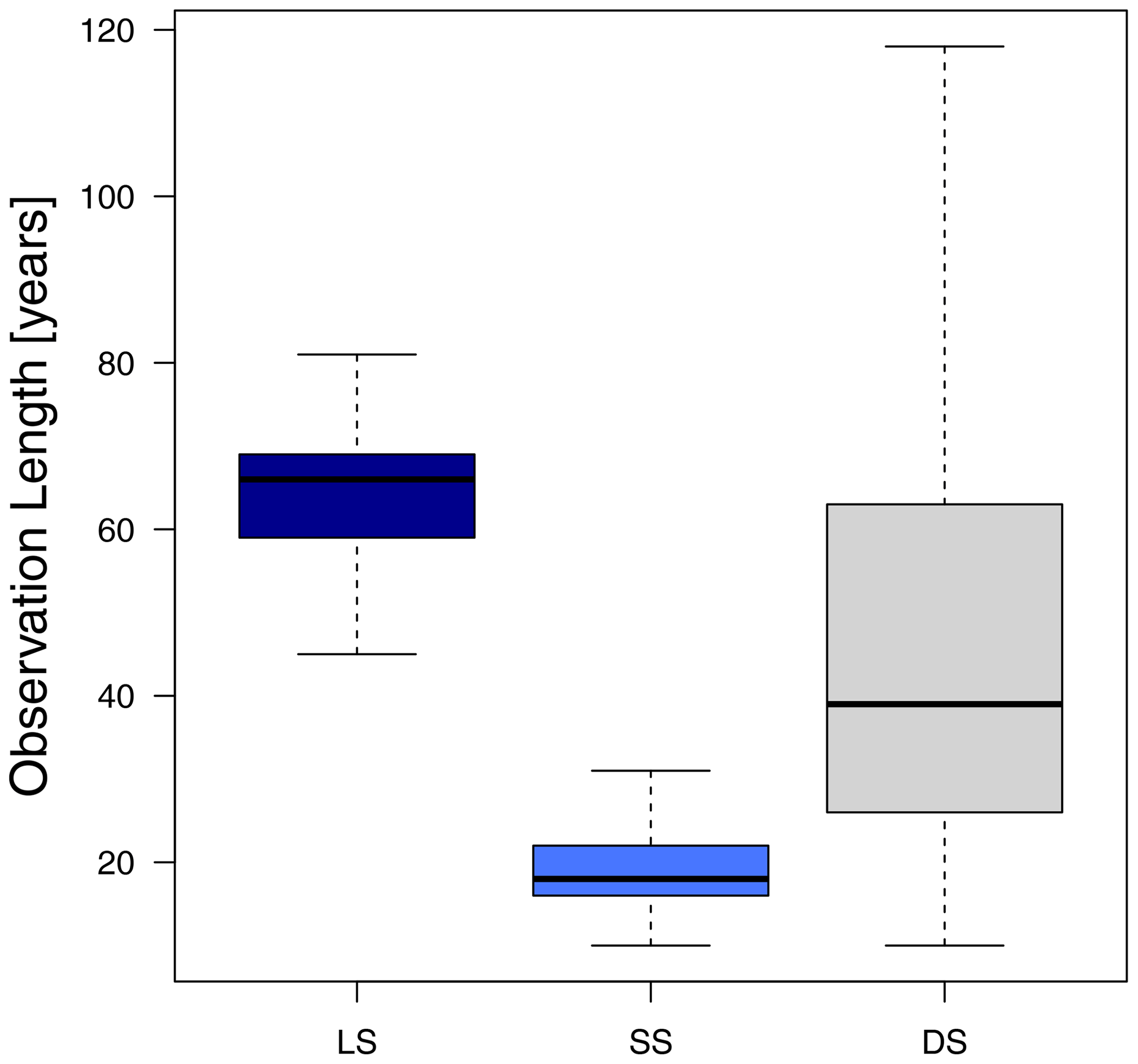
Figure 2Observation length of all stations grouped according to the three available data types in Germany: long series (LS), short series (SS) and daily series (DS).
Table 1Number of stations for each of the available data types in Germany: long series (LS), short series (SS) and daily series (DS).
2.2 Temporal disaggregation of the daily series
The daily dataset (DS) is much denser than both long and short ones and includes even longer observation periods than the LS dataset. If it is possible to disaggregate these data reliably, this will considerably increase the number of support points for the regionalisation of DDF curves. For the considerations presented here, the so-called cascade model first introduced by Olsson (1998) is employed. A more extensive parameterisation is implemented in the method according to Lisniak et al. (2013), which corresponds to a transfer of the Olsson method to a 3-fold distribution. To generate sub-hourly data, disaggregation parameters are derived from the RADOLAN weather radar time series of each grid cell (Bartels et al., 2004), and the daily observed volumes are disaggregated for the given durations as shown in Table 2. It is important to note that due to the parameterisation using RADOLAN data, no parameter regionalisation is required, so that the parameter-rich disaggregation procedure in the Lisniak variant can be used. Moreover, 30 realisations of disaggregated data were generated for each duration, in order to capture the uncertainty due to the disaggregation. It was evaluated that the relative error does not improve significantly for more than 30 realisations, as also reported in Müller and Haberlandt (2018), therefore only 30 realisations of disaggregated data were used in this study.
Table 2The disaggregation scheme applied to the daily data (DS) to obtain rainfall volumes at the given durations.

To understand what errors can be introduced to the DDF curves when employing this disaggregation scheme, a direct comparison was conducted between the long series (LS) and the disaggregated daily series (DS) for the return periods 1, 10, 20, 50 and 100 years. For each station, duration level and return period, the relative error is calculated as the difference between the disaggregated and the original rainfall quantile. The resulting deviations for all stations are shown in Fig. 3. The results indicate that at the longer duration levels (> 6 h), the DDF curves are captured quite well, and the main disadvantage of the disaggregation model (as expected) is for the very short duration. Below the duration of 4 h, there is a clear tendency to underestimate the extremes from LS, up to a median underestimation of 14 % at the 30 min duration level. At the duration of 15 min, a weakening of the underestimation is observed, which is probably due to the instationarity in the original series identified in Sect. 2.4 below, which predominates only at duration levels up to 15 min. Thus, it is expected for the DS disaggregation scheme to be more useful for the longer duration extremes than the short ones, particularly the extremes at sub-hourly durations.
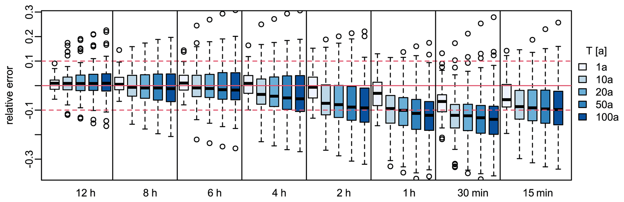
Figure 3The relative error (−) of the disaggregated daily station data (30 realisations) based on radar parameterisation for different return periods and duration levels: (+) sign indicates overestimation, while (−) sign is the underestimation of extremes. Different blue shades indicate the error at different return periods (in years) as shown in the legend (eg. 1a is a 1-year return period).
2.3 Annual maximum series for each dataset
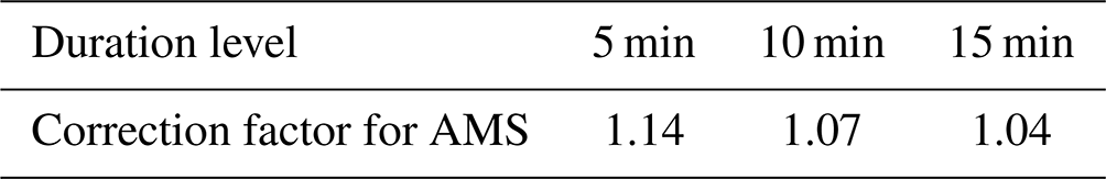
Using the 5 min time series, the annual maximum series (AMS) is derived based on the calendar year for the duration levels of 5 min, 10 min, 15 min, 30 min, 1 h, 2 h, 6 h, 12 h, 1 d, 2 d, 3 d and 7 d. A moving window with the length of each duration level is used to derive the annual maxima, considering a dry duration of 4 h to ensure that the maxima selected in December and January of 2 consecutive years are independent from one another. Additionally, following the guidelines given by DWA (2012), a scaling of the durations of 5, 10 and 15 min AMS with the factors given in Table 3 is performed. This is done to avoid the systematic underestimation of rainfall extremes at a short duration caused by the deviation between (i) the start of the actually largest rainfall sum of duration D, and (ii) the fixed starting time of the 5 min time series (employed here).
Table 3Correction factors for annual maximum series (AMS) of short duration according to the DWA-531 (DWA, 2012).
2.4 Homogenisation of long and short dataset
First, plausibility and homogeneity checks were performed on the long and short datasets, herein referred to respectively as the long series (LS) and short series (SS). An initial analysis of possible trends based on the quantile regression (Koenker, 2005) was carried out for the monthly 5 min maximum intensities of the long series (LS). This method was chosen, as, in comparison to the classical regression, it is considerably more robust and it allows to obtain regression results for different non-exceedance probabilities. In Fig. 4, the quantiles for the non-exceedance probabilities τ= 0.5 (i.e. median), 0.8, 0.9 and 0.95 are considered. Quantile regressions for the four selected τ with time as the explanatory variable are implemented separately for each of the 133 measurement points. Each dashed line corresponds to a measuring station and each colour to a non-exceedance probability. Trend-like changes in the monthly 5 min maxima are visible with slopes that increase with τ. To understand why this trend is present in almost all long series, we investigated whether these instationarities are more trend-like or jump-like, with the latter assuming that the timing of jumps is associated with sensor changes in the measuring network. In the long series, a total of 19 different sensor types are distinguished simply by two states: analogue or digital.
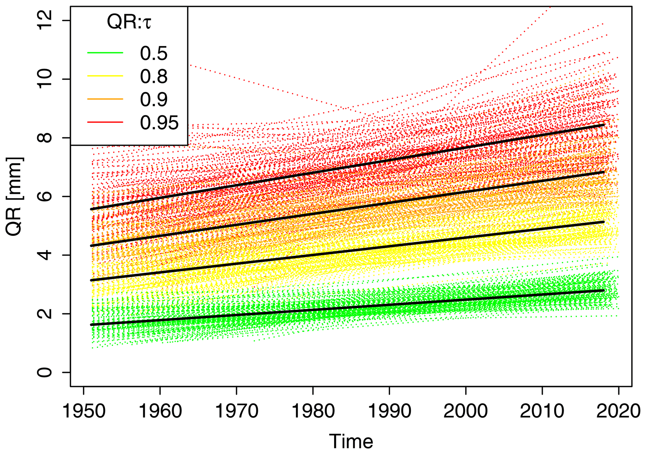
Figure 4Quantile regression (QR in mm) on monthly maximum 5 min rainfall intensities for the long series (LS) for different non-exceedance probabilities τ (shown in coloured dashed lines and in the legend). The fitted quantile regression is shown with a solid black line.
A test for trend, jump or stationarity based on instationary extreme value analysis (Coles, 2001) was performed for all 133 LS. We tested for a linear trend in the location parameter vs. jump at the date of the sensor change from analogue in the early years to digital in the later years in the location parameter vs. stationarity. The decision was based on the Akaike information criterion. The results for different duration levels (x axis) are shown in Fig. 5 on the left. It is obvious that the majority of instationarities at short duration levels is better explained as a jump (with a mostly positive sign) in the data. A possible reason could lie in the limited ability of analogue gauges to register abrupt intensity changes, so that the total amount of precipitation falling in a short time interval may not be fully detected by analogue sensors, leading to positive jumps at sensor changes from analogue to digital. However, as a counterargument, the so-called “step–response–error” that occurs with digital sensors could also be considered (see e.g. Licznar et al., 2015). Since the instationarities are usually jumps and not trends, a simple homogenisation of the data to a uniform sensor type is possible by raising the mean value of the digital sensor type (DVWK, 1999). This jump correction is applied separately for each station and duration level. The results of applying the instationarity test to the homogenised series are shown in Fig. 5 on the right. It can be seen that this approach can eliminate the instationarities at short duration levels significantly. About 30 % of the stations show instationarities (either trend or jump), while the remaining part is considered stationary. Since only a small part of the stations show instationarities, a stationary extreme value analysis is performed here.
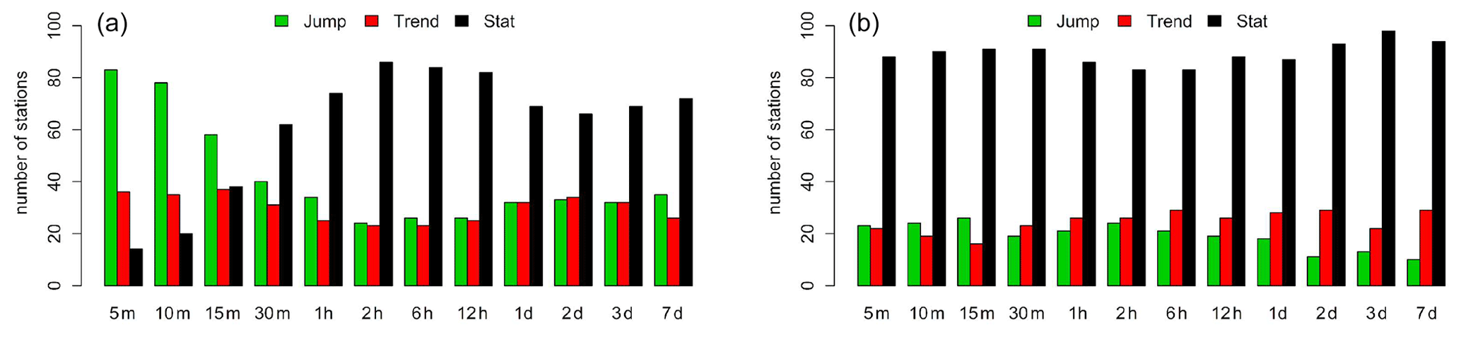
Figure 5Number of long series (LS) stations that show stationarity (stat) vs. instationarity (either jump- or trend-like) at different duration levels following the instationary extreme value analysis; (a) before jump elimination and (b) after jump elimination between analogue and digital sensors.
3.1 Local estimation of extreme value statistics
3.1.1 Reference approach
Here, the generalised extreme value (GEV) probability distribution is used for the statistical analysis of extreme rainfall and the derivation of the local DDF curves, described as the following:
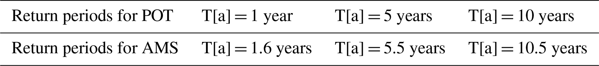
where μ is the location, σ is the scale and γ is the shape parameter. If the shape parameter is greater than zero, heavy-tail behaviour is present (GEV type II); if the shape parameter is less than zero, then it is the reverse Weibull distribution with no-tail behaviour (Coles, 2001). The GEV parameters are fitted to the AMS of each duration level and station separately, based on the L-moments method. For this purpose, the R package “lmomco” was used (Asquith, 2021). A prior investigation in our study revealed that the L-moment approach led to more stable results than the method of maximum likelihood. The shape parameter was either estimated or fixed at 0.1 for the estimation of return periods up to 100 years, approximately following the recommendation from Koutsoyiannis (2004a, b) for an estimation of return periods up to 100 years (γ ∼0.1) and in a prior analysis conducted on LS series. Based on the parameters obtained, the quantiles of return periods T1a, T10a, T20a, T50a and T100a were derived. Since the AMS approach tends to underestimate quantiles at low return periods (T[a] < 10 years), a correction of the AMS return periods according to the DWA-531 regulations with factors given in Table 4 was performed.
Table 4Correction of the return periods (T[a]) when fitting the GEV to the annual maximum series (AMS) adapted from DWA (2012).
Because the parameters are fitted separately on each duration, quantile crossing may occur. Quantile crossing happens when the extreme rainfall volumes of a fixed probability (T[a] = 100 years) are not increasing with longer duration levels. Figure 6 shows for different return periods, T1a, T10a, T20a, T50a and T100a, the number of stations affected by these crossings for the empirically calculated quantiles (left) and the quantiles fitted with the general extreme value (GEV) distribution (right). The empirical quantiles are calculated according to Hyndman and Fan (1996). It is clear that the number of stations with this problem increases significantly for larger return periods. Especially the SS dataset exhibits frequent crossing in the empirical quantiles at long duration levels (D≥24 h). Here, the volumes of the duration D72 h and D168 h are lower than the extremes of D24 h. With the GEV-fitted quantiles, significantly more stations show quantile crossings than with the empirically calculated quantiles. These problems occur for all return periods, however they are more frequent for the return periods T50a and T100a. In order to avoid such problems, two different methods are applied and compared here: the approach presented by Koutsoyiannis et al. (1998) and the approach presented by Fischer and Schumann (2018). These two methods are described below.
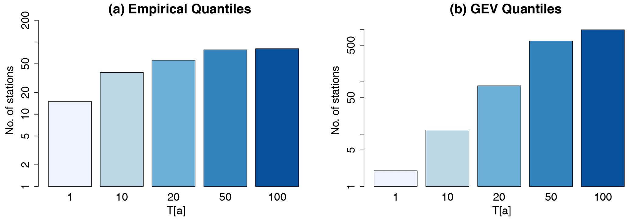
Figure 6Number of all stations at a 5 min resolution (for both short and long series) for different return periods (T[a]) showing quantile crossings in the empirically calculated quantiles (a) and the GEV-fitted quantiles (b) with increasing duration.
3.1.2 Koutsoyiannis approach
Koutsoyiannis et al. (1998) consider the intensity as a function of the duration level through two parameters (θ, η), and the generalised intensity can be calculated from duration specific intensity as described below:
where i is the generalised intensity in mm h−1, id is the intensity in mm h−1 observed at each duration level, d is the duration level in hours, and θ and η are the Koutsoyiannis parameters optimised for each station. Through this relationship, a generalisation of the AMS intensities over all the chosen duration levels is possible. The parameters θ (larger than 0) and η (within the range 0 to 1) are estimated for each station by minimising the Kruskal–Wallis statistic as indicated in Koutsoyiannis et al. (1998). The advantage of this optimisation method lies in its non-parametric character and robustness, as the Kruskal–Wallis statistics are not affected by the presence of extreme values in the sample. Once the parameters θ and η are determined, the generalised intensities from all duration levels are pooled together (as the main assumption is now that they follow the same distribution) and a GEV distribution is fitted to this sample by the methods of L-moments. Lastly, to obtain DDF curves, the quantiles at specific return periods are estimated from the fitted GEV distribution and are divided by the term bd in Eq. (2) (depending on θ and η parameters and the duration level). This joint estimation of parameters over all durations should not only avoid the quantile crossings but also make the estimation of the DDF more robust.
3.1.3 Fischer–Schumann approach
In contrast to Koutsoyiannis who treats the intensities of AMS as a function of the duration, Fischer and Schumann (2018) propose an approach based on the GEV distribution, where the generalised GEV parameters are monotonically dependent on the GEV parameters determined for each duration level. Thus, as a first step, the GEV parameters (as in Eq. 1) are estimated from the L-moment methods for each duration level at each station, and then through a nonlinear regression (with two parameters α and β), each GEV parameter is related to the different duration levels as indicated by the following equations:
where d is the duration level in 5 min, are the GEV parameters of each duration, while α and β are the regression coefficients with αμ,ασ > 0, , β≥0. The parameters are obtained by nonlinear least square minimising. In addition to the shape parameter dependency shown in Eq. (3), three alternative approaches are considered: a constant shape parameter over all durations, a shape parameter fixed at 0.1, and a quadratic relationship as in Eq. (4).
where P1 and P2 are estimated spanning across all stations, and a is a station-specific optimised parameter.
3.2 Regionalisation of extreme value statistics
The local parameters estimated for each station (GEV parameters and generalisation parameters) make the base dataset for the regionalisation of the extreme rainfall statistics. Each of these parameters is regionalised independently based on the regionalisation methods explained below, and later on, DDF maps for each duration and return period of interest are generated. The overall procedure for regionalisation is given in Fig. 7a, and the regionalisation methods are given in Fig. 7b. The regionalisation approaches were compared only for four parameters (see parameters of KO.FIX in Table 5), as these four parameters were selected as the most appropriate for local DDF estimation in Sect. 4.1.
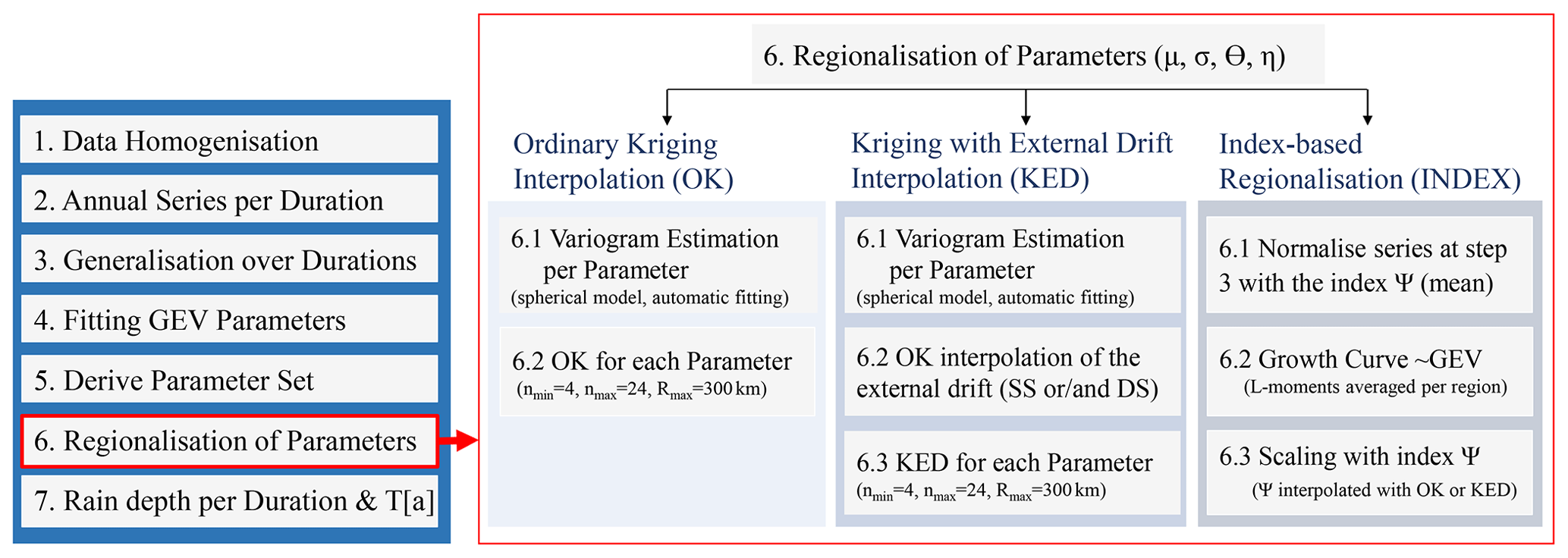
Figure 7(a) The step-by-step methodology applied here from the given point datasets to the final regionalised rainfall depths over all durations and return periods (T[a]) in Germany; (b) a detailed procedure for step 6 – regionalisation (shown in red) only for the parameters of KO.FIX (see Table 5) carried out with different methods (ordinary kriging – left, external drift kriging – middle, and index-based regionalisation – right). The parameters interpolated are the GEV (location μ and scale σ) and Koutsoyiannis (θ and η) parameters. For both kriging methods, for each parameter, first a spherical variogram is estimated (step 6.1) and the interpolation is performed (steps 6.2 or 6.3) with the given nmin, nmax and Rmax which are the kriging parameters for minimum, maximum number of neighbours and maximum radius for neighbour search. For index-based regionalisation, first the generalised series obtained in step 3 are normalised with the index Ψ (step 6.1), next a regional GEV growth curve for each homogeneous region is derived based on regional L-moments (step 6.2), and finally the quantiles at each duration are rescaled with the index Ψ (step 6.3).
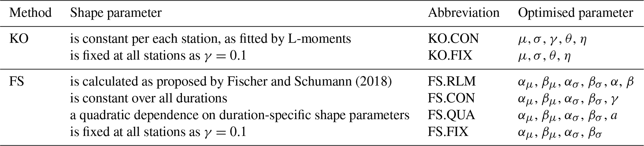
Table 5A review of the methods and the different calculation of the shape parameter investigated for the local statistics, where KO stands for Koutsoyiannis and FS for the Fischer and Schumann framework.
3.2.1 Ordinary kriging interpolation
The regionalisation of extreme value statistics for Germany will first be carried out with ordinary kriging (OK) interpolation. Here, the extreme rainfall parameters are interpolated independently. The flow chart for this interpolation technique is shown in Fig. 7b. Ordinary kriging is widely used for interpolation due to its simplicity in comparison to other kriging methods. The expected value of the random process being investigation (E) is treated as constant in space (as per Eq. 5), whereas the increase in variance of the target variable at any two locations (u and u+h) depends only on the distance h. This increase in the variance is represented by the semi-variogram function γ(h) (here called variogram). Therefore, in the first step, the empirical variogram is estimated by discrete point observations according to Eq. (6).
where N is the number of any two observed data pairs (uiand uj) at distance h. Since the empirical variograms are not continuous functions, theoretical variograms must be fitted to the observed values. To describe the spatial variance of the data, several theoretical variogram models can be used and fitted to the empirical variogram using the least squares method. For the interpolation of rainfall extremes, a spherical variogram (as per Eq. 7) is chosen as more appropriate (Kebaili Bargaoui and Chebbi, 2009).
where c0 is the nugget, c the sill, and a is the range of the variogram. The variogram describes the spatial variability of the target variable and the average dissimilarity between a known and unknown location. Once the theoretical variogram is known, it can be used as a basis for interpolating the statistical properties on a 5 km grid. This grid resolution was chosen for two reasons; first it is consistent with the HyRas product from the German Weather Service that uses the same resolution, second it is a compromise between the coarsest and finest legible resolution computed from the given density of long series (LS) (the reference for this study) following the suggestions of Hengl (2006). The interpolation is done as indicated in Eq. (8), the variable at an unknown location (Z′) is estimated by the weighted average of the nearby known locations (Zui).
where the weights (λi) are derived from the theoretical variogram, and n is the number of selected neighbours. The R package “gstat” is used to fit the variograms and interpolate the variables (Pebesma, 2004). An advantage of ordinary kriging interpolation is that the weights are determined in such a way that the difference between the estimated and the observed values is zero on average. However, this can lead to the interpolated variable being smoothed in space. Different theoretical variograms were previously investigated, i.e. exponential, Gaussian and spherical, with the spherical model together with a nugget effect showing the best fit for the case study. The fitting of the variogram model parameters for different data types and experiments is done automatically by a weighted least square fit. Since the automatic fit relies on the initial values of the model parameters, we defined the initial values with trial and error, and accepted a fit that was adequate qualitatively. Figure 8 illustrates the empirical and theoretical normalised variograms for interpolation of the GEV and Koutsoyiannis parameters (after the method KO.FIX shown in Table 5) estimated from the three main datasets available: long series (LS), short series (SS) and 30 realisations of disaggregated daily series (DS). Note that the variograms are normalised in order to ensure a comparison between the different datasets. From this figure, a clear difference between the spatial dependency of different datasets, due to different station densities and settings, is visible. The long and short series (LS and SS) exhibit a similar relationship with each other for the GEV parameters (μ and σ) but distinguish either in the nugget value (c0) or the range (a), whilst the daily disaggregated series clearly exhibits a different nugget (c0), range (a) and even sill (c). The differences between the datasets are less visible in the spatial dependencies of the Koutsoyiannis parameters (θ and μ), where the three datasets differ slightly in nugget and range. Particularly the spatial dependency of the scale parameter is captured quite differently by the three datasets. Here, LS and SS are differing mainly at the nugget value, where LS has a smaller value than the SS series, suggesting that the spatial structure of the scale parameter from SS is smoother than that of LS. On the other hand, the DS datasets exhibit a completely different variogram for the scale parameter, suggesting that the extremes of the high return period (influenced mainly by the scale parameter) will have different spatial structures than those of the LS and SS series.

Figure 8Empirical (dots) and fitted (solid lines) spherical theoretical variograms for the GEV (μ – location and σ – scale) and Koutsoyiannis (θ and η) parameters estimated by three different datasets (long series LS in dark blue, short series SS in light blue and disaggregated daily series DS in grey).
3.2.2 Kriging with external drift interpolation
In the kriging with external drift (KED), the expected value E of the target variable Z at any location u is linear-dependent on secondary variables Y, and thus Eq. (5) takes the form of Eq. (9). Here the secondary variables (or the external drifts) reflect the spatial trend of the target variable. Theoretically, the variogram for KED interpolation is computed from the residuals between the target and the secondary variables. Here for simplicity the OK variograms are used instead, since, as shown in Delrieu et al. (2014), they can produce very similar results to the KED one.
where Y represents k secondary variables from 1 to m that are used as an external drift, b0 is the interception of the linear dependency, and bk is the coefficient for each k drift. For this study, different site characteristics (i.e. elevation) were investigated as external drift, however as indicated by the cross-correlation between the target variables (in this case, the four parameters describing the local statistics) and the site characteristics, the linear dependency between them is not high (see Appendix Fig. A1). Therefore, here only interpolated local parameters from the short and/or daily series are used as external drift information.
3.2.3 Index-based regionalisation
The regionalisation of extreme rainfall statistics in Germany is also carried out using the index method according to Hosking and Wallis (1997). The index method was originally developed for the regionalisation of flood quantiles, however it found a wide application also for the regionalisation of extreme rainfall statistics. By pooling information in statistically homogeneous regions, a more robust estimate of extreme rainfall statistics can be made, and based on each defined region, the information can be transferred to other unobserved points. A homogeneous region exists if the distribution functions have the same shape at all points in the region. The homogeneity indicator H1 presented by Hosking and Wallis (1997) is typically used to determine homogeneous regions. If the H1 is lower than 1, the region is said to be homogeneous, if it is between 1 and 2 the region may be heterogeneous, and if it is higher than 2, the region is definitely not homogeneous. Here different site characteristics like the latitude, longitude, elevation and long-term annual average of sunshine duration and mean annual precipitation were used as inputs to define homogeneous regions. Based on a k-clustering approach (Ward, 1963), nine homogeneous regions were identified and are shown in Fig. 9. The obtained homogeneous regions were tested for homogeneity for each data type combination and, as visible from Fig. A2 in Appendix, all values are below 1, meaning that the regions selected are homogeneous and can be used for the index-based regionalisation. Note that the generalised statistics over all the durations from Sect. 3.1 are used as inputs for the homogeneity test. The R package “nsRFA” is used to obtain the homogeneous regions (Viglione et al., 2020). In order to find an appropriate number of clusters, different numbers of clusters between 2 and 20 are tested and compared based on the homogeneity indicator H1 and whether they were spatially continuous and physically reasonable. The maximum number of clusters of 20 was chosen to ensure a sufficient number of stations and thus a sufficient number of observation years per region (Hosking and Wallis, 1997).

Figure 9Nine homogeneous regions implemented here for the index-based regionalisation. The regions shown here are a generalisation of the k-cluster results to account for spatial consistency.
Once the homogeneous regions are determined, the different local statistics are normalised by a scaling factor, the index. In contrast to the previous regionalisation techniques discussed so far, the index-based regionalisation has an extra step – the normalisation of the general intensities with the index (performed in step 3 in Fig. 7 on the left), which in this case is the mean generalised intensity. Next, the local L-moments are estimated on the basis of the normalised annual series, and regional L-moments are derived for each region weighting the local L-moments according to their time series length. Finally, a GEV growth curve is fitted for each region via the regional L-moments. The R package “lmomRFA” was employed for the application of the index method (Hosking and Wallis, 1997). In the final step, by back-scaling the normalised extreme rainfall for all observed and unobserved points in the homogeneous region, estimates can be made about the extreme rainfall as a function of the duration (based on regional averaged values of observed θ and η) and the return period (based on the regional GEV growth curve). The geostatistical interpolation of the index makes it possible to transfer the extreme value statistical evaluations to unobserved points within the region.
3.3 Performance assessment and comparison
3.3.1 Local performance assessment
For the local estimation of the GEV parameters that describe the extreme rainfall over all the selected duration levels, two different approaches were consulted: from Koutsoyiannis et al. (1998) (herein referred to as KO) and from Fischer and Schumann (2018) (herein referred to as FS). Before carrying on with the regionalisation, it is important to investigate which of the methods is more adequate for the estimation of the GEV parameters over all the duration levels. Moreover, the two methods not only distinguish their approach of generalisation across duration, but they also include different variations on the calculation of the GEV shape parameter (γ). A review of the methods and shape parameters is given in Table 5, together with the respective optimised parameter set for each case. The obtained parameters for different datasets are shown in the Appendix in Fig. A3 for KO and in Fig. A4 for FS.
The performance of the methods and the respective case of shape parameters as illustrated in Table 5 is evaluated only at the location of the long series (LS) by comparing the normalised quantiles over all durations for return periods T1a, T10a, T20a, T50a and T100a with the GEV quantiles calculated separately at each duration level. Here the percentage RMSE (as per Eq. 10) was employed to assess the errors of the selected cases at each duration level and station with respect to the GEV duration specific quantiles as follows:
where i represents each of the five selected return periods, T[a], varying from 1 to 100 years, st varies from 1 to 133 available long series, RDgen,st corresponds to the derived rainfall depth from the generalisation method of duration d, RDd,st is the derived rainfall depth from the GEV quantiles at duration d, and the is the mean rainfall depth from the GEV quantiles at a duration d averaged over the return periods. Alternatively, the error for each return period and station can also be calculated by Eq. (10) by swapping the d with T[a] and where is the mean rainfall depth from the GEV quantiles at return period T[a] averaged over the duration levels d (from 5 min up to 7 d, therefore i changes from 1 to 12).
Since the GEV quantiles fitted per duration level cannot be considered the ground truth, a non-parametric bootstrap is performed when estimating the parameters of each method, in order to investigate the sampling uncertainty of derived DDF values. For this purpose, 100 randomisations of the observations were conducted and the uncertainty range of the derived rainfall depths is computed as follows:
where nCI95width is the 95 % confidence interval width and mean is the average of rainfall depth obtained from 100 realisations and expressed for each long series (LS) location st, duration level d and return period T[a]. The smaller the uncertainty range, the more robust the estimated parameters for the high return periods. Based on the two performance criteria, percentage RMSE and nCI95width, all the methods in Table 5 are compared to evaluate the best one for the estimation of rainfall DDF curves. The best method is selected as the one with the lowest RMSE and nCI95width. The results of this comparison are given in Sect. 4.1.
3.3.2 Spatial performance assessment
In order to check which of the regionalisation approaches provides the best results, a leave-one-out cross-validation was carried out at the locations of the long series (LS 133 stations). For each approach, the rainfall depth (RD) is determined from the return periods T1a, T10a, T20a, T50a and T100a and the selected duration levels. After regionalisation, the regionalised rainfall depths are compared with the local generalised GEV quantiles (here assumed to be the truth). The short series are omitted from the cross-validation, as no reliable extreme value statistics can be carried out for large return periods due to the very short observation length. The quality of the regionalisation approaches is evaluated using the following criteria:
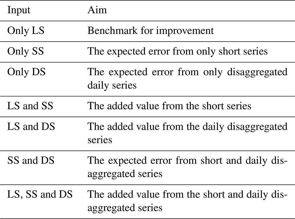
where the d varies from 1 to D= 12 for each duration level between 5 min and 7 d, T[a] is the return period, st the respective long series (LS) station, RDregional corresponds to the regionalised rainfall depth, RDlocal the locally derived rainfall depth from the generalised GEV function, and the is the mean local rainfall depth averaged over the durations. The cross-validation only at the location of the LS makes it possible to investigate the value that the short (SS) and the disaggregated daily series (DS) are adding to each regionalisation method. For this purpose, the regionalisation methods are run first only with the LS as input, and the performance of such an application is considered the benchmark for improvement. Later on, the SS and DS are added stepwise as input to the regionalisation, in order to assess the improvement they introduce towards the benchmark. Additionally, one can calculate the expected performance when only the short or/and the disaggregated daily series are available and not the long one. An overview of these experiments and their aim is given in Table 6.
Table 6Overview of the experiments performed with different data sets for each regionalisation method, where SS is the short series, LS is long series and DS is the disaggregated daily series.
A directed comparison of the performance criteria between the different experiments and the benchmark is calculated here as per Eq. (15) as follows:
where perfref,T[a] is the performance criteria calculated for each return period T[a] as per Eqs. (12)–(14) from the scenario with only LS as input, and perfnew,T[a] is the performance of any other combination of input data as per Eqs. (12)–(14). A positive value for this criterion indicates an improvement in performance in comparison to the only LS scenario, while a negative value indicates a deterioration. Note that the signs of the nominator are exchanged in the case of the improvement of the NSE. It is also important to emphasise that the scenario ref corresponds to the best regionalisation method with only LS as the input, namely the ordinary kriging of LS based on the results of Sect. 4.2.
Finally, based on different combinations of the available series (data types) as external drift in the kriging interpolation may help to shed light on which combination of the data is more useful for the regionalisation of the rainfall DDF values. Here the data to be used as external drift are first interpolated with ordinary kriging. A description of these different combinations for the KED interpolation is given in Table 7. The performance of the different combinations is evaluated only at the location of the LS, and the best integration is selected based on the highest improvement in comparison to regionalisation with only LS as the input.
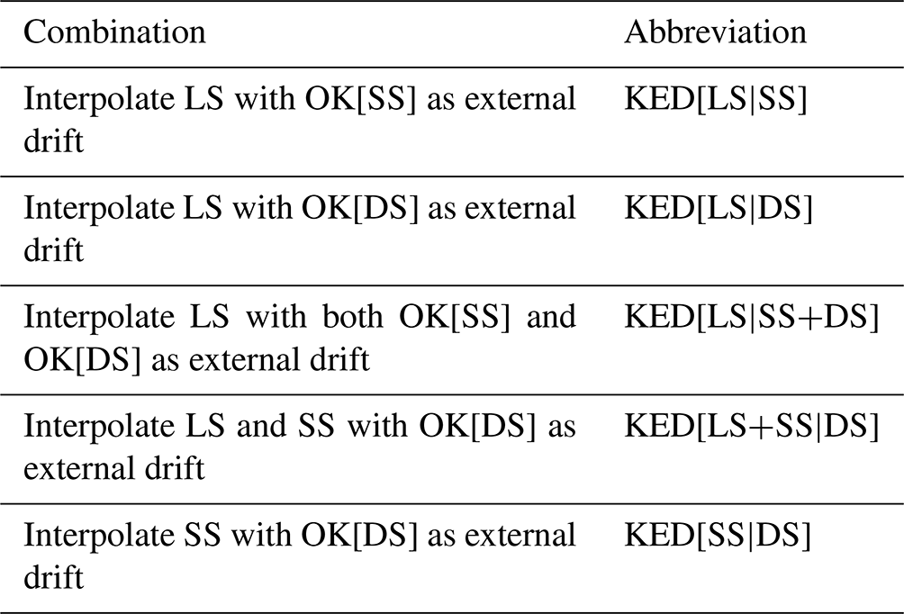
Table 7Overview of different integration of data types in kriging with external drift (KED) interpolation, where SS is the short series, LS is the long series and DS is the disaggregated daily series. Pooling the data together with the same importance is represented by a (+) sign, whereas priority importance (integration through an external drift) is represented by the (|) sign.
4.1 Local estimation of extreme statistics
Figure 10 illustrates the local percentage RMSE of each method in comparison to the duration-specific quantiles (as per Eq. 10). The upper row of Fig. 10 shows the percentage RMSE calculated for each location and duration level over all the return periods, and the lower row of Fig. 10 shows the percentage RMSE calculated for each location and return period over all the duration levels. The results from Fig. 10 in the upper row indicate that the KO approaches (both fixed and station constant shape parameter) have an almost constant RMSE over all durations under the value of 10 %. On the other hand, the FS approaches tend to have similar or smaller RMSE for the longer duration (median RMSE under 8 %), but they are not able to represent well enough the very short durations. For the FS approaches, the RMSE median for duration levels up to 60 min is higher than 10 %, with the 5 min RMSE being the highest (between 25 % and 45 %). The results from Fig. 10 in the lower row illustrate that all the approaches manifest higher errors witha higher return period. Both of the KO approaches (fixed and station constant shape) show very similar behaviour. The KO.FIX performs slightly worse (1 %–4 % higher RMSE) than the KO.CON, but this is expected as the duration GEV fitted per duration independently favours the KO.CON (as the shape parameter is let free for the GEV parameter fitting). The FS approaches perform very similarly to one another, however here contrary to the KO.FIX approach, the performance of the FS.FIX seems better than the other approaches. Overall, the KO approaches have the priority at shorter durations, and they can capture the volumes at specific durations better than the FS approaches. On the other hand, the FS approaches can capture better extremes at longer durations. A unanimous selection is not yet possible from the obtained results so far, because the local GEV duration-specific parameters may not represent the ground truth.
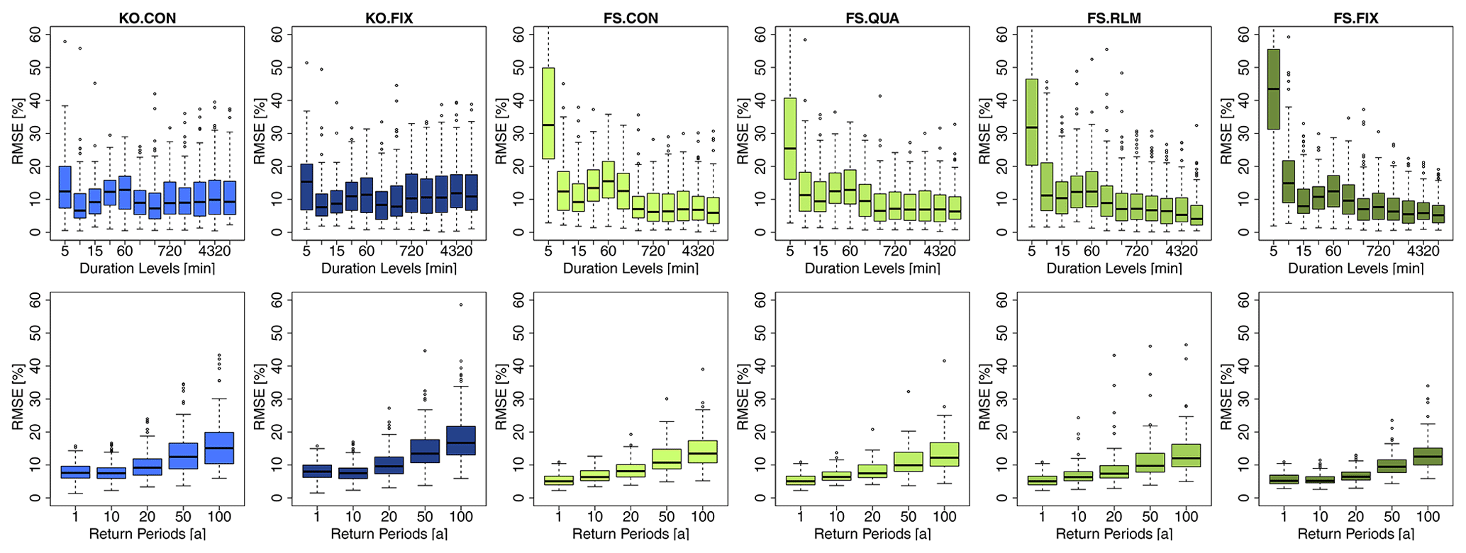
Figure 10RMSE (%) performance of the given generalisation methods over all the long series (LS) in comparison to the duration-specific GEV quantiles grouped in the upper row for different duration levels (calculated per station over return periods, T[a]), and the lower row for different return periods (calculated per station over duration levels). The overview of the methods shown here is given in Table 5.
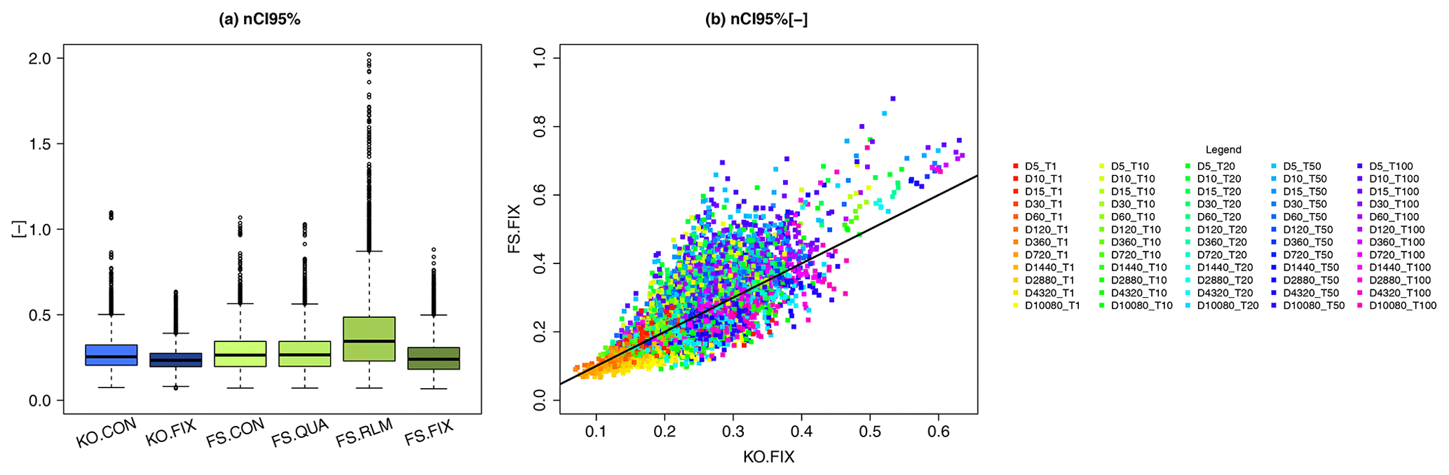
Figure 11On the left is the comparison of the normalised 95 % confidence interval width [–] for the methods and shape parameters selected for the generalisation of the DDF values over all the durations (see Table 5 for a summary of the methods). On the right is a direct comparison of the normalised 95 % confidence interval width [–] for KO.FIX (x axis) with FS.FIX (y axis) for each duration D and return period T[a] (shown in different colours).
To analyse which approach estimates more stable and representative parameters, a non-parametric bootstrap was performed (with 100 random realisations), and it served as a basis for assessing the 95 % confidence interval width of the obtained DDF values. Fig. 11 on the left shows the normalised 95 % confidence interval widths (nCI95width) for the rainfall depth (as per Eq. 11) estimated for each of the selected approaches. A high value of the nCI95width indicates that the bootstrap yields very variable rainfall depths, and hence a higher uncertainty is associated with the method. Contrarily a low value of the nCI95width indicates that the rainfall depths have low variation across the random realisations, and thus the obtained DDF curves are considered more stable or robust. The results shown in Fig. 11 indicate that the KO.FIX exhibits the lowest variation (median nCI95width ∼ 0.23), followed by FS.FIX (∼0.25), and by KO.CON, FS.CON and FS.QUA with slightly higher variations (respectively ∼0.3). It is interesting to see that the FS.RLM has a median nCI95width∼0.3 but can reach extreme values up to 2. Fig. 11 on the right shows the scatterplot of nCI95width obtained from the KO.FIX (x axis) and FS.FIX (y axis) for different duration levels and return periods (shown with different colours) at the LS locations. Except for very low return periods (T1a), FS.FIX exhibits on average higher values of nCI95width than KO.FIX. Based on these results, the KO.FIX (Koutsoyiannis framework with shape parameter fixed at 0.1) was chosen as the best method and was used for the regionalisation of the DDF curves. The advantages of the KO.FIX are that: (1) it represents all duration levels similarly and fairly, (2) the parameter estimation is more robust than any of the other methods and (3) it uses a known and well-established method for the estimation of the DDF curves.
4.2 Regionalisation of extreme statistics
As discussed in the Sect. 4.1, the AMS at different duration levels was normalised according to the Koutsoyiannis approach and the GEV parameters were fitted to the grouped generalised intensities. The shape parameter was kept fixed at 0.1. Ordinary kriging (OK) and index-based (INDEX) regionalisation were run first only with the LR data as input, to decide about which of the two approaches will serve as a benchmark. A direct comparison based on Eq. (15) is then performed for each of the selected performance criteria (where new is OK and ref is INDEX), to compute the improvement or deterioration of OK with only LS data compared to the INDEX. The median values for each return period, performance criteria and method are given in Table 8. Here it becomes clear that the kriging approach exhibits a lower RMSE for all return periods, worse BIAS for high return periods and slightly better NSE than the index method. Based on these results, the kriging with LS as input (KRIGE[LS]) is used as a benchmark for calculating the improvement in performance by adding additional data types. Apart from the performance, the other advantage of kriging is that it is more of a “pure” method, as it interpolates independently the four parameters, while the index approach is a “mixture” between the regional growth curve estimation, averaging θ and η parameters and kriging to interpolate the index. For this reason, one may prefer the kriging regionalisation, as the errors are mainly from the kriging system, while the index method includes errors from the kriging system and from regional and averaged parameters.
Table 8Median performance improvement/deterioration (%) of ordinary kriging (OK) versus index-based (INDEX) regionalisation calculated for different data as per Eq. (15) (where new is OK and ref in INDEX), when only long series (LS) are used as input. The performance is obtained by cross-validation over 133 LS stations. The colour green (+) indicates better performance by OK, and red (–) indicates better performance by INDEX.

4.2.1 Best regionalisation for different data combinations
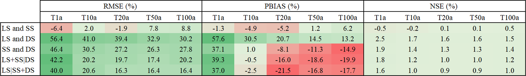
Kriging and index-based regionalisation was then performed for each data type experiment given in Table 6, and the cross-validation results for the 133 LS locations were compared to the benchmark (KRIGE[LS]) selected before as the best regionalisation with only LS as an input. To enable an easy comparison between the two regionalisation methods, the difference between the improvements achieved between the kriging and the index-based regionalisation in comparison to the benchmark was calculated for each of the 133 LS locations. The median differences (in percent) for each data type experiment over the 133 locations for each performance criteria and return period are given in Table 9. A positive difference (dark green shade) means that the improvements reached by the kriging interpolation are higher than the index-based regionalisation. A negative difference (red shade) means the opposite. The data are combined by two operators: either (+), referring to pooling of the datasets together with same importance (the parameters and the index are interpolated with ordinary kriging), or (|), referring to a linear relationship between the datasets (priority importance) where the parameters and the index are interpolated through external drift kriging.
Table 9Median difference between kriging and index-based improvements calculated for different data as per Eq. (15). The median is computed from 133 stations. The data used as input are short series (SS), long series (LS) and disaggregated daily series (DS) and combined either with same importance (+) or with priority importance (|). The positive difference shown in green shades indicates that kriging introduces bigger improvements towards the benchmark than the index-based regionalisation. The negative differences shown in red shades indicate that the index-based regionalisation has the bigger improvements.
The results from Table 9 indicate that for most of the cases the kriging interpolation brings higher improvements to the benchmark than the index-based regionalisation. Exceptions are the regionalisation with only SS, LS+SS, SS|DS, LS+SS|DS and LS|SS+DS where the index-based regionalisation exhibits a median 2 %–12 % higher PBIAS improvement for higher return periods than the kriging interpolation. However, for these cases, the RMSE and the NSE improvements are much higher for the kriging regionalisation. Therefore, it can be concluded that overall the kriging interpolation yields better results than the index-based regionalisation (lower RMSE and higher NSE), but may suffer depending on the combination of data types from slightly higher PBIAS. Also, it has to be mentioned that when grouping the daily disaggregated time series directly (operator +) with the other data types (either LS and SS), the kriging performs up to 100 % better than the index-based regionalisation. This suggests that the parameters from the disaggregation do not follow the same regions or growth curve as the high-resolution data (LS and SS), thus a kriging interpolation seems a more reasonable choice for integrating daily disaggregated series (DS).
The results of Table 9 give a direct comparison between kriging and index-based regionalisation; nevertheless, as they are relative to each case, they do not give any information if ordinary kriging or external drift kriging yields better regionalisation results. For this purpose, the difference of improvements between KED and OK were calculated and shown as median over the 133 LS locations in Table 10. A positive difference (green shade) means that the improvements reached by KED are higher than the OK interpolation. A negative difference (red shade) means otherwise. The results show that overall, the KED exhibits higher RMSE and NSE improvements than the OK, but the KED tends to have lower PBIAS improvements than the OK. When only the high-resolution datasets are present (LS and SS), the KED behaves better than OK mainly for high return periods (50–100 a); when LS and DS are present, KED clearly outperforms the OK. For all the remaining cases the OK outperforms the KED only for the PBIAS of high return periods.
Table 10Median difference between external drift kriging (KED) and ordinary kriging (OK) improvements calculated for different data as per Eq. (15). The median is computed from 133 stations. The data used as input are short series (SS), long series (LS) and disaggregated daily series (DS) and combined either with same importance (+) or with priority importance (|). The positive difference shown in green shades indicates that KED introduces bigger improvements towards the benchmark than the OK. The negative differences shown in red shades indicate that the OK regionalisation has the bigger improvements.
4.2.2 Best data integration for regionalisation
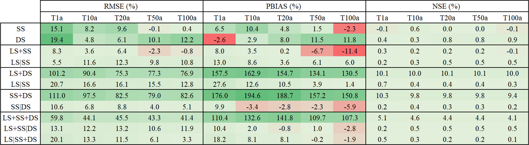
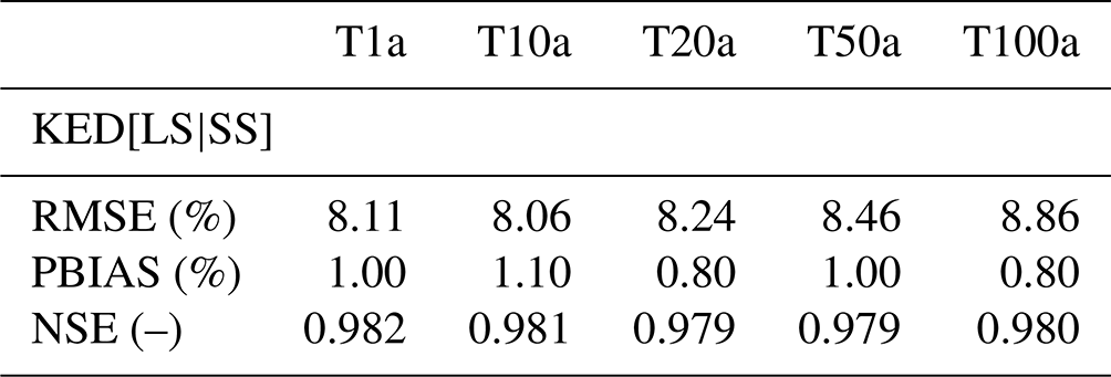
So far, the external drift kriging interpolation has shown superiority for regionalising DDF curves in comparison to the index-based and ordinary kriging regionalisation. Nevertheless, the question still remains: what is the best combination of the datasets for regionalising the DDF curves in Germany? Here it is interesting to see if all the three available datasets are useful for regionalisation or if single or dual networks are enough. For this purpose, the performance improvement exhibited by different combinations of the data types in KED (as per Table 7) in comparison to the benchmark are visualised in Fig. 12. Note that since there are 30 realisations of DS data, a boxplot is illustrating the performance spread over these 30 realisations. This affects regionalisation methods where DS data are present, otherwise a single line indicates the performance of the regionalisation. For very low return periods (T1a), the integration of all data types of the form KED[LS+SS|DS] brings the best performance, with RMSE and BIAS up to 20 % smaller and NSE 0.7% higher. For return period T10a, the KED[LS|SS], KED[LS|DS] and KED[LS+SS|DS] perform very similarly: some random realisation from the disaggregated daily series (DS) introduces high improvement but also low values, even though the median over the 30 realisations is at the same level as the KED[LS|SS] one. For high return periods (T100a), KED[LS|SS] introduces the highest improvement in all three performance criteria. Actually KED[LS|DS] is the second-best option, however the median over the 30 realisations is either lower or equal to the performance of the KED[LS|SS]. There are few realisations that introduce the highest improvements for RMSE and BIAS, nevertheless the computation time for the disaggregation scheme and the fitting of the Koutsoyiannis approach is also a disadvantage of using the DS dataset. So finally, the kriging interpolation of the long network (LS) with the short network (SS) as an external drift is chosen as an optimal method for the regionalisation of the GEV and Koutsoyiannis parameters. Table 11 indicates the median performance criteria (RMSE, PBIAS, NSE) for different return periods reached by this method (KED[LS|SS]). The expected deterioration in performance when the long series is not present in comparison to the best method selected for regionalisation (KED[LS|SS]) is given in Table A1 in the Appendix.

Figure 12Median performance improvements towards the benchmark from regionalising on different data combinations, as per Table 7, in kriging with external drift, where SS is the short series, LS is the long series and DS is the disaggregated daily series, combined either with the same importance (+) or with priority importance (|).
Table 11Median cross-validation performance over 133 long series (LS) stations for the final selected regionalisation method (KED[LS|SS]) at different return periods (T[a]).
The three different datasets implemented here are distinguished from one another based on the parameter values (as shown in Fig. A3 of the Appendix) and on the spatial dependency and variograms, as shown in Fig. 8. When fixing the shape parameter to 0.1, the location and Koutsoyiannis parameters of LS and SS are in a similar range, and the main difference is seen at the scale parameter (where the SS has higher values of the scale parameter than LS). This gives a tendency of the short durations to estimate bigger rainfall volumes for higher return periods. This behaviour is also in agreement with that reported by Madsen et al. (2017) who used a generalised Pareto distribution also with a fixed shape parameter. Typically, this is treated by index-based regionalisation, where extremes within a region are pooled together to estimate the DDF curves at an unknown location as done in Requena et al. (2019). However, we show here that integrating the LS and SS with external drift kriging, hence accounting for the spatial dependency of the extremes, delivers better performance than grouping them together in the index-based regionalisation (also valid for the LS and DS integration).
4.3 Final product and discussion
The obtained maps, on a 5 km raster, for the four regionalised parameters (location parameter μ, scale parameter σ, Koutsoyiannis θ and η parameters) with the KED[LS|SS] approach are illustrated in Fig. 13. Here the shape parameter is fixed to 0.1 for the whole of Germany, which is very similar to results obtained by Ulrich et al. (2021) (shape parameter as 0.11 from the annual GEV approach), and it validates our approach. The spatial distribution of the location GEV parameter (μ) follows partly the elevation information, with higher values in the southeast where the German Alps are located. The scale GEV parameter (σ) values are independent of the elevation, with a high localised value near to Münster city. In 2014, there was a very extreme event in Münster which has affected the statistics of the station located in the vicinity. Currently it is not clear how to handle these singular extraordinary events in extreme value analysis in an optimal way. Both Koutsoyiannis parameters (θ and η) show similar spatial patterns with lower values in the Alps and other mountainous regions and on the northwestern coast. These parameters exhibit higher variability in space than the GEV location or scale parameters. Overall, the spatial distribution of η parameter follows the spatial structure of the annual rainfall sum in Germany, the distribution of the location (μ) parameter follows the information from the elevation, while the scale (σ) and θ parametera do not seem to be influenced by any climatologic or site characteristic. This is also seen in Van De Vyver (2012), where annual rainfall and elevation is concluded as important covariates, mainly for the location (μ) parameter, while the scale (σ) parameter did not have meaningful covariates, and the shape parameter did not show any spatial structure but was kept constant over Belgium. These results agree to a certain extent with the results obtained here. However, the rainfall statistics extracted from short or daily series are considered as more important than the annual rainfall (which itself is an interpolation from point observation). Thus, interpolation of long datasets should include extreme statistics from short or daily series rather than annual rainfall as additional information.

Figure 13Obtained interpolated maps from the KED[LS|SS] for each of the parameters: location parameter μ, scale parameter σ, Koutsoyiannis θ and η parameters. The shape parameter γ is kept constant at 0.1. The black lines illustrate the borders of German federal states.
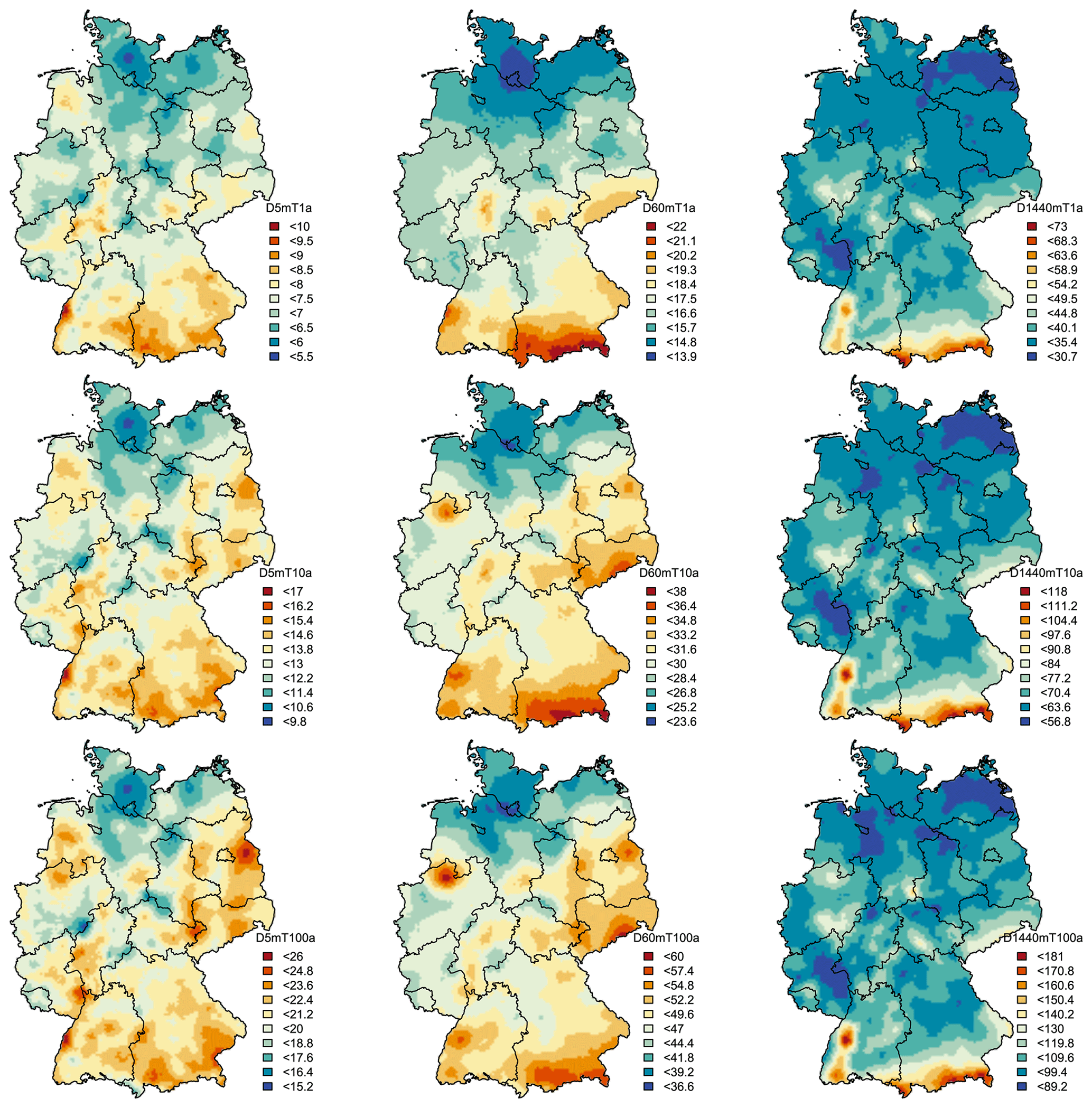
Figure 14Obtained design rainfall (mm) maps for the whole of Germany from the KED[LS|SS] regionalisation approach derived for different durations (D= 5, 60 and 1440 min): first row – return period T[a] = 1 year, second row – return period T[a] = 10 years and third row – return period T[a] = 100 years. The black lines illustrate the borders of German federal states.
With these four interpolated maps, together with the shape parameter fixed at 0.1, DDF curves can be obtained for any location in Germany. A few examples of design rainfall maps for duration levels 5 min, 1 h and 1 d, and return period T[a] = 1, 10 and 100 years, are given in Fig. 14. For short durations (i.e. D=5 min), the spatial distribution of rainfall extremes is independent from the elevation and becomes more erratic with higher return periods. This is in accordance with the fact that the convective extreme events can happen anywhere and are very low correlated with the orography. With increasing duration level, the relationship between orography and extreme rainfall becomes stronger. As for instance in D=1 h, the influence of the alpine regions is visible, which becomes even stronger for the duration of D=1 d. In the existing KOSTRA maps, all durations are dependent on elevation. Here, the elevation itself did not show much effect on the scale (σ) and θ parameter, only to some extent on the location (μ) and η parameter. This means that the extremes of longer duration (affected by the η parameter) and of low return period (affected by the location parameter) will show a pattern resembling the elevation. This is not true for short durations (affected by the θ parameter) and high return periods (affected by the scale parameter). This also agrees with other studies that report a weak dependence of short duration rainfall (shorter than 1 or 2 h) with the elevation in Germany (Lengfeld et al., 2019). Lastly, the kriging interpolation as implemented here opens the possibility to capture better uncertainty – not only the sample uncertainty, which is typically done by bootstrapping the points statistics, but also accounting for the spatial structure of extremes by considering spatial simulations. Following this study and the best chosen method here, an extensive uncertainty analysis is given in Shehu and Haberlandt (2022), whose results propose that DDF estimates with KED[LS|SS] are more precise near to the location of long series (LS) and less precise in regions far from long series (LS).
In this study, the use of three ground measuring types in Germany was investigated for the estimation of design rainfall maps. These data types included a long high-resolution dataset with long observations at 5 min time steps from 60–70 years, a short high-resolution dataset with short observations also at 5 min time steps from 10 to 20 years, and a daily dataset with observations varying from 10 to 100 years. The purpose of the work was to review different methods for the estimation and regionalisation of the DDF curves and to investigate the value and the best integration of different data types for estimating DDF curves in unobserved locations. The results will provide the basis for a new update of the design storm maps for Germany, the KOSTRA-2023. First, the long analogous and recent digital high-resolution networks were homogenised by performing a jump correction, with the jumps coinciding with sensor type changes. Second, the daily dataset was disaggregated to sub-hourly durations based on a cascade model parameterised according to Olsson (1998) and Lisniak et al. (2013) from the RADOLAN data in Germany. Third, annual maximum series (AMS) were derived for each station available in the three datasets for duration levels ranging from 5 min to 7 d. This represents the main database for the present investigation. Two methods were investigated for local estimation of rainfall extreme statistics, adopted from Koutsoyiannis et al. (1998), and Fischer and Schumann (2018), and three different regionalisation approaches (ordinary kriging, external drift kriging and index-based regionalisation) were investigated for the spatial estimation of DDF curves in Germany. The conclusions derived, by considering the long high-resolution dataset as the truth, are summarised as follows.
Both methods for local estimation of the rainfall extreme statistics behave quite similarly in capturing the local duration-specific rainfall depths. Nevertheless, the estimation of parameters through the Koutsoyiannis approach is more robust in terms of data sampling uncertainties. Particularly, the Koutsoyiannis approach combined with a generalised extreme value (GEV) distribution with a fixed shape parameter value at 0.1 exhibited the highest robustness with tolerable decline in precision. Therefore, four parameters were used to describe the local statistics of extreme rainfall: the location and scale GEV parameters and the two Koutsoyiannis parameters θ and η. These four parameters represent the basis for the testing of different scenarios and regionalisation approaches.
When only the long high-resolution dataset is present, both ordinary kriging and index-based regionalisation perform similarly, with ordinary kriging showing slightly better median performance. This result remains true also for other data combination settings, with kriging methods exhibiting lower RMSE and NSE, but slightly higher PBIAS than the index-based regionalisation. The only case where the index-based regionalisation has superiority against kriging is when only short high-resolution series are present.
When more than two data types are available, kriging with external drift seems more adequate for the parameter interpolation than ordinary kriging, at least regarding the RMSE and NSE performance.
A combination of long and short high-resolution series improves the performance of regionalisation considerably (up to 15 % for T[a] = 100 years), but only when the datasets are combined with external drift kriging. Here the parameters from the short series are first interpolated with ordinary kriging, which later on serve as an external drift for the kriging interpolation of the parameters from the long series. This combination gave overall the best results at least for return periods higher than 10 years.
A combination of the long high-resolution and daily dataset improves the performance of regionalisation up to 10 % being the second-best method for regionalisation. Here also the best regionalisation was the external drift kriging, with the ordinary kriging interpolation of daily parameters serving as an external drift.
A combination of the three data types improves the regionalisation considerably (up to 20 %) only for low return periods (shorter or equal to 10 years).
Overall, the best method for the regionalisation of the DDF curves in Germany was the kriging interpolation of the long sub-hourly stations with the short sub-hourly stations as an external drift. On average, this approach exhibited 8 %–9 % RMSE (increasing with the return period) and up to 1 % BIAS (decreasing with the return period) when compared to the locally estimated DDF curves.
The cross-validation implemented here can only describe the accuracy of the regionalisation methods when compared to the local estimation, but it does not say much about the precision of the predictions. Thus, it is important to perform an uncertainty analysis, which should include not only the local estimation of sample statistics (briefly discussed here) but also the spatial uncertainty of the kriging interpolation. The integration of spatial uncertainty in the DDF design storms of Germany is investigated and discussed in Shehu and Haberlandt (2022). Further improvements of the methodology might include the validation of the methods on a distinguished region. It has to be noted that the majority of the reference stations in Germany are located in the lowlands, thus the mountainous areas may be under-represented. It would be interesting to investigate if daily data or other site characteristics (like the elevation) are improving the performance of the chosen method in these regions. However, should one decide to perform region-specific regionalisation, special care should be paid to the continuity of DDF values at the borders of the regions. Lastly, these conclusions are valid mainly for Germany, where dense networks are present. The advantage of each dataset or approach may still change depending on the station density or study area location.
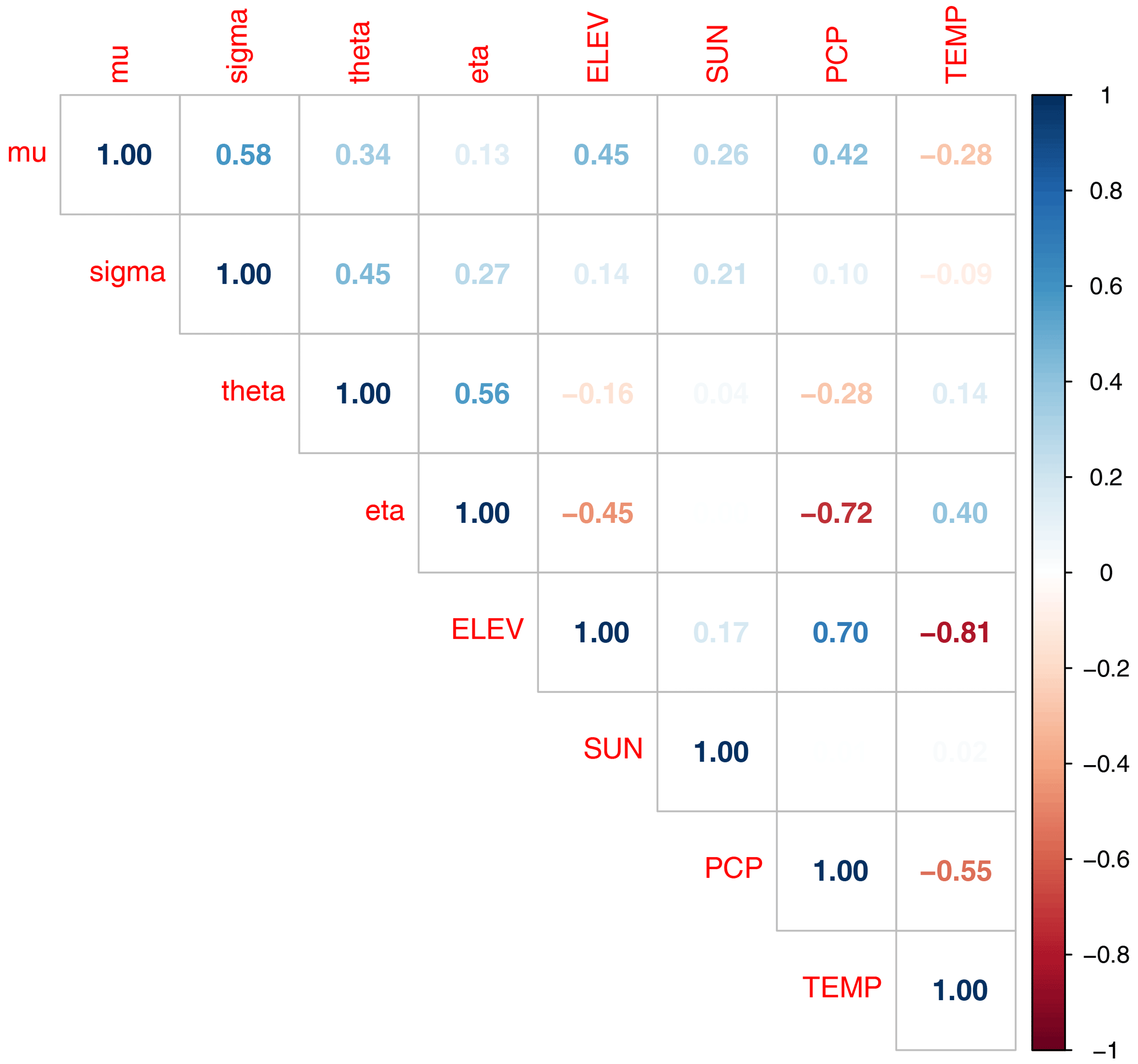
Figure A1Cross-correlation between the selected local parameters (Koutsoyiannis and GEV parameters) for regionalisation and useful site characteristics that might act as an external drift information. μ (mu) is the GEV location parameter, σ (sigma) the GEV scale parameter, and θ (theta) and η (eta) the Koutsoyiannis parameters. ELEV is short for elevation information, SUN is short for long-term average of annual sunshine duration, PCP is short for long-term average of annual rainfall amount, and TEMP is short for the long-term average of annual mean temperature.
Table A1Obtained deterioration (–) or improvement (+) towards the best regionalisation technique (KED[LS|SS]) when no long series are available (LS) and the regionalisation is performed based on short series (SS), disaggregated daily series (DS), or on both SS and DS.

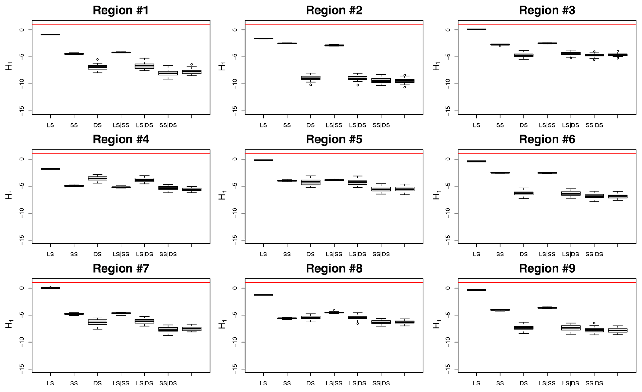
Figure A2The homogeneity index (H1) computed for each of the ninth selected regions for each of the dataset combinations.
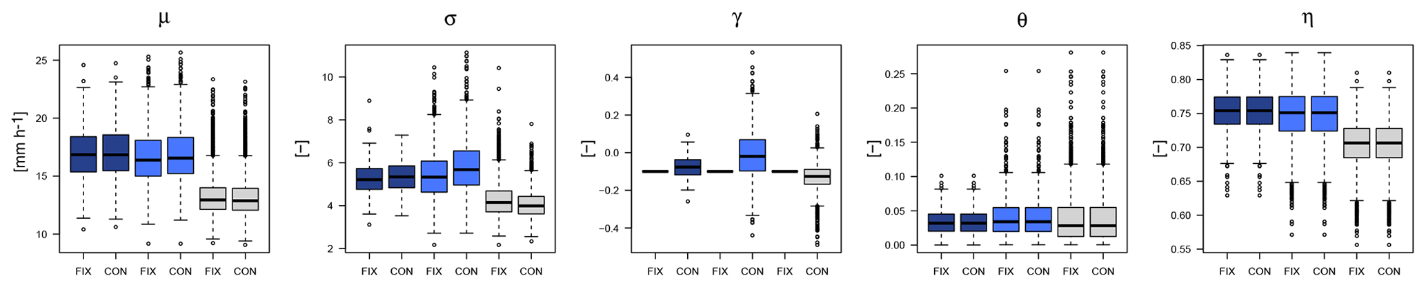
Figure A3Koutsoyiannis parameters obtained for each dataset (LS in dark blue, SS in light blue and DS in grey) when fixing the shape parameter to 0.1 for all stations (FIX) or constant over all durations per station (CON).
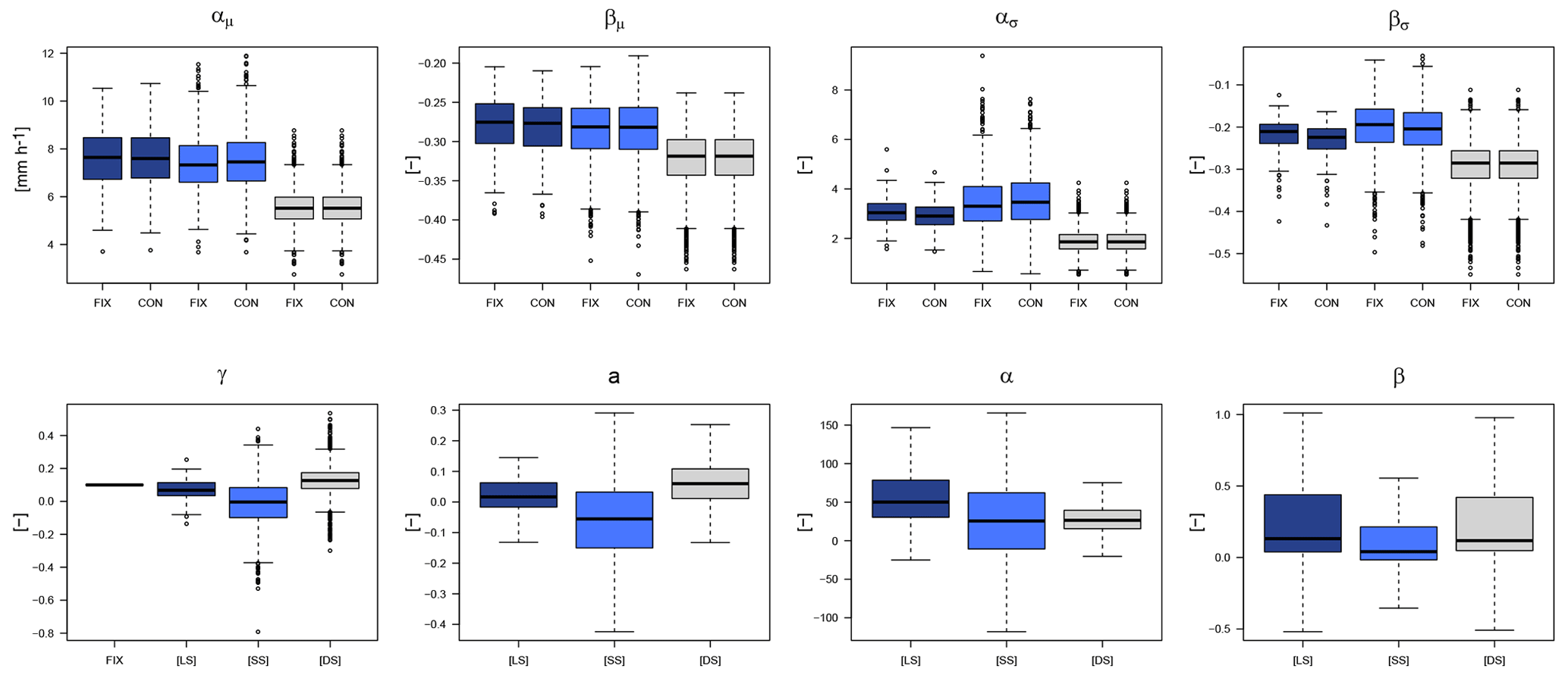
Figure A4Fischer–Schumann parameters obtained for each dataset (LS in dark blue, SS in light blue and DS in grey) when fixing the shape parameter to 0.1 (FIX) or constant over all durations per station (CON).
The daily and the short sub-daily network, RADOLAN radar data, and the other meteorological variables have been made publicly available by the German Weather Service (DWD) and can be accessed at https://opendata.dwd.de/climate_environment/CDC/ (German Weather Service (DWD), 2023). The long sub-daily network has been digitalised and provided by the DWD. All R codes can be provided by the corresponding authors upon request.
The supervision and funding for this research were acquired by UH and WW. The study conception, design and methodology were performed by all authors, while the software, data collection, derivation and interpretation of results were handled mainly by BS and WW (with support from the other authors). BS prepared the original draft, which was revised by all authors.
The contact author has declared that none of the authors has any competing interests.
Publisher's note: Copernicus Publications remains neutral with regard to jurisdictional claims in published maps and institutional affiliations.
The results presented in this study are part of the research project “Investigating Different Methods for Revising and Updating the Heavy Rainfall Statistics in Germany (MUNSTAR)”, funded by the German Ministry of Agriculture and Environment Mecklenburg-Vorpommern and the Federal State Funding Programme “Water, Soil and Waste”, who are gratefully acknowledged. We are also thankful for the provision and right to use the data from the German National Weather Service (Deutscher Wetterdienst DWD), more specifically Thomas Deutschländer and Thomas Junghänel. Lastly, we would like to thank Paweł Licznar and Juraj Parajka for their comments that improved the final version of the paper.
This research was funded by the German Ministry of Agriculture and Environment Mecklenburg-Vorpommern and the Federal State Funding Programme “Water, Soil and Waste”.
This paper was edited by Carlo De Michele and reviewed by Paweł Licznar and Juraj Parajka.
Asquith, W. H.: Lmomco—L-moments, censored L-moments, trimmed L-moments, L-comoments, and many distributions: R package version 2.3.7, August May 3, 2021, https://cran.r-project.org/package=lmomco, last access: 30 August 2021.
Bara, M., Kohnová, S., Gaál, L., Szolgay, J., and Hlavčová, K.: Estimation of IDF curves of extreme rainfall by simple Scaling in Slovakia, Contrib. to Geophys. Geod., 39, 187–206, 2009.
Bárdossy, A. and Pegram, G.: Combination of radar and daily precipitation data to estimate meaningful sub-daily point precipitation extremes, J. Hydrol., 544, 397–406, https://doi.org/10.1016/J.JHYDROL.2016.11.039, 2017.
Bartels, H., Weigl, E., Reich, T., Lang, P., Wagner, A., Kohler, O., Gerlach, N., and MeteoSolutions GmbH: Projekt RADOLAN – Routineverfahren zur Online-Aneichung der Radarniederschlagsdaten mit Hilfe von automatischen Bodenniederschlagsstationen (Ombrometer), Offenbach am Main, Abschlussbericht, https://www.dwd.de/RADOLAN (last access: 20 March 2022), 2004.
Berndt, C., Rabiei, E., and Haberlandt, U.: Geostatistical merging of rain gauge and radar data for high temporal resolutions and various station density scenarios, J. Hydrol., 508, 88–101, https://doi.org/10.1016/j.jhydrol.2013.10.028, 2014.
Borga, M., Vezzani, C., and Fontana, G. D.: Regional Rainfall Depth-Duration-Frequency Equations for an Alpine Region, Nat. Hazards, 36, 221–235, 2005.
Burn, D. H.: A framework for regional estimation of intensity-duration-frequency (IDF) curves, Hydrol. Process., 28, 4209–4218, https://doi.org/10.1002/hyp.10231, 2014.
Cannon, A. J.: Non-crossing nonlinear regression quantiles by monotone composite quantile regression neural network, with application to rainfall extremes, Stoch. Environ. Res. Risk A., 32, 3207–3225, https://doi.org/10.1007/s00477-018-1573-6, 2018.
Ceresetti, D., Ursu, E., Carreau, J., Anquetin, S., Creutin, J. D., Gardes, L., Girard, S., and Molinié, G.: Evaluation of classical spatial-analysis schemes of extreme rainfall, Nat. Hazards Earth Syst. Sci., 12, 3229–3240, https://doi.org/10.5194/nhess-12-3229-2012, 2012.
Coles, S.: Basics of Statistical Modeling, in: An Introduction to Statistical Modeling of Extreme Values, Springer Series in Statistics, Springer, London, https://doi.org/10.1007/978-1-4471-3675-0_2, 2001.
Delrieu, G., Wijbrans, A., Boudevillain, B., Faure, D., Bonnifait, L., and Kirstetter, P. E.: Geostatistical radar–raingauge merging: A novel method for the quantification of rain estimation accuracy, Adv. Water Resour., 71, 110–124, https://doi.org/10.1016/J.ADVWATRES.2014.06.005, 2014.
De Salas, L. and Fernández, J. A.: “In-site” regionalization to estimate an intensity-duration-frequency law: a solution to scarce spatial data in Spain, Hydrol. Process, 21, 3507–3513, https://doi.org/10.1002/hyp.6551, 2007.
Durrans, S. R. and Kirby, J. T.: Regionalization of extreme precipitation estimates for the Alabama rainfall atlas, J. Hydrol., 295, 101–107, https://doi.org/10.1016/j.jhydrol.2004.02.021, 2004.
DVWK: Statistische Analyse von Hochwasserabflüssen, Deutscher Verband für Wasserwirtschaft und Kulturbau, Tech. Rep. H. 251, Bonn, Germany, p. 62, 1999.
DWA: Arbeitsblatt DWA-A 531: Starkregen in Abhängigkeit von Wiederkehrzeit und Dauer, DWA Arbeitsgruppe HW 1.1e, Hennef, Deutschland, https://de.dwa.de (last access: 20 March 2022), 2012.
Fischer, S. and Schumann, A. H.: Berücksichtigung von Starkregen in der Niederschlagsstatistik, Hydrol. Wasserbewirts., 62, 248–256, https://doi.org/10.5675/HyWa_2018,4_2, 2018.
Forestieri, A., Lo Conti, F., Blenkinsop, S., Cannarozzo, M., Fowler, H. J., and Noto, L. V.: Regional frequency analysis of extreme rainfall in Sicily (Italy), Int. J. Climatol., 38, e698–e716, https://doi.org/10.1002/joc.5400, 2018.
German Weather Service (DWD): https://opendata.dwd.de/climate_environment/CDC/, last access: 6 March 2023.
Goudenhoofdt, E., Delobbe, L., and Willems, P.: Regional frequency analysis of extreme rainfall in Belgium based on radar estimates, Hydrol. Earth Syst. Sci., 21, 5385–5399, https://doi.org/10.5194/hess-21-5385-2017, 2017.
Gupta, V. K. and Waymire, E.: Multiscaling properties of spatial rainfall and river flow distributions, J. Geophys. Res., 95, 1999–2009, https://doi.org/10.1029/JD095iD03p01999, 1990.
Hengl, T.: Finding the right pixel size, Comput. Geosci., 32, 1283–1298, https://doi.org/10.1016/j.cageo.2005.11.008, 2006.
Holešovský, J., Fusek, M., Blachut, V., and Michálek, J.: Comparison of precipitation extremes estimation using parametric and nonparametric methods, Hydrolog. Sci. J., 61, 2376–2386, https://doi.org/10.1080/02626667.2015.1111517, 2016.
Hosking, J. R. M and Wallis, J. R.: Regional Frequency Analysis: An Approach Based on L-moments, Cambridge University Press, UK, https://doi.org/10.1017/cbo9780511529443, 1997.
Hyndman, R. J. and Fan, Y.: Sample Quantiles in Statistical Packages, Am. Stat., 50, 361–365, https://doi.org/10.1080/00031305.1996.10473566, 1996.
Johnson, F. and Sharma, A.: Design Rainfall, in Handbook of Applied Hydrology – Second Edition, edited by: Singh, V. P., McGraw-Hill, New York, chap. 125, ISBN 9780071835091, 2017.
Kebaili Bargaoui, Z. and Chebbi, A.: Comparison of two kriging interpolation methods applied to spatiotemporal rainfall, J. Hydrol., 365, 56–73, https://doi.org/10.1016/j.jhydrol.2008.11.025, 2009.
Koenker, R.: Quantile Regression (Econometric Society Monographs), Cambridge, Cambridge University Press, https://doi.org/10.1017/CBO9780511754098, 2005.
Koutsoyiannis, D.: Statistics of extremes and estimation of extreme rainfall: I. Theoretical investigation, Hydrolog. Sci. J., 49, 575–590, https://doi.org/10.1623/hysj.49.4.575.54430, 2004a.
Koutsoyiannis, D.: Statistics of extremes and estimation of extreme rainfall: II. Empirical investigation of long rainfall records, Hydrolog. Sci. J., 49, 591–610, https://doi.org/10.1623/hysj.49.4.591.54424, 2004b.
Koutsoyiannis, D., Kozonis, D., and Manetas, A.: A mathematical framework for studying rainfall intensity-duration-frequency relationships, J. Hydrol., 206, 118–135, https://doi.org/10.1016/S0022-1694(98)00097-3, 1998.
Lengfeld, K., Winterrath, T., Junghänel, T., Hafer, M., and Becker, A.: Characteristic spatial extent of hourly and daily precipitation events in Germany derived from 16 years of radar data, Meteorol. Z., 28, 363–378, https://doi.org/10.1127/metz/2019/0964, 2019.
Licznar, P., De Michele, C., and Adamowski, W.: Precipitation variability within an urban monitoring network via microcanonical cascade generators, Hydrol. Earth Syst. Sci., 19, 485–506, https://doi.org/10.5194/hess-19-485-2015, 2015.
Lisniak, D., Franke, J., and Bernhofer, C.: Circulation pattern based parameterization of a multiplicative random cascade for disaggregation of observed and projected daily rainfall time series, Hydrol. Earth Syst. Sci., 17, 2487–2500, https://doi.org/10.5194/hess-17-2487-2013, 2013.
Madsen, H., Arnbjerg-Nielsen, K., and Mikkelsen, P. S.: Update of regional intensity-duration-frequency curves in Denmark: Tendency towards increased storm intensities, Atmos. Res., 92, 343–349, https://doi.org/10.1016/j.atmosres.2009.01.013, 2009.
Madsen, H., Gregersen, I. B., Rosbjerg, D., and Arnbjerg-Nielsen, K.: Regional frequency analysis of short duration rainfall extremes using gridded daily rainfall data as co-variate, Water Sci. Technol., 75, 1971–1981, https://doi.org/10.2166/wst.2017.089, 2017.
Marra, F., Nikolopoulos, E. I., Anagnostou, E. N., Bárdossy, A., and Morin, E.: Precipitation frequency analysis from remotely sensed datasets: A focused review, J. Hydrol., 574, 699–705, https://doi.org/10.1016/j.jhydrol.2019.04.081, 2019.
Müller, H. and Haberlandt, U.: Temporal rainfall disaggregation using a multiplicative cascade model for spatial application in urban hydrology, J. Hydrol., 556, 847–864, https://doi.org/10.1016/J.JHYDROL.2016.01.031, 2018.
Olsson, J.: Evaluation of a scaling cascade model for temporal rain- fall disaggregation, Hydrol. Earth Syst. Sci., 2, 19–30, https://doi.org/10.5194/hess-2-19-1998, 1998.
Paixao, E., Auld, H., Mirza, M. M. Q., Klaassen, J., and Shephard, M. W.: Regionalization of heavy rainfall to improve climatic design values for infrastructure: case study in Southern Ontario, Canada, Hydrolog. Sci. J., 56, 1067–1089, https://doi.org/10.1080/02626667.2011.608069, 2011.
Papalexiou, S. M.: Unified theory for stochastic modelling of hydroclimatic processes: Preserving marginal distributions, correlation structures, and intermittency, Adv. Water Resour., 115, 234–252, https://doi.org/10.1016/j.advwatres.2018.02.013, 2018.
Papalexiou, S. M. and Koutsoyiannis, D.: Battle of extreme value distributions: A global survey on extreme daily rainfall, Water Resour. Res., 49, 187–201, https://doi.org/10.1029/2012WR012557, 2013.
Pebesma, E. J.: Multivariable geostatistics in S: The gstat package, Comput. Geosci., 30, 683–691, https://doi.org/10.1016/j.cageo.2004.03.012, 2004.
Requena, A. I., Burn, D. H., and Coulibaly, P.: Pooled frequency analysis for intensity–duration–frequency curve estimation, Hydrol. Process., 33, 2080–2094, https://doi.org/10.1002/hyp.13456, 2019.
Shehu, B. and Haberlandt, U.: Uncertainty estimation of regionalised depth–duration–frequency curves in Germany, Hydrol. Earth Syst. Sci. Discuss. [preprint], https://doi.org/10.5194/hess-2022-254, in review, 2022.
Smithers, J. C. and Schulze, R. E.: A methodology for the estimation of short duration design storms in South Africa using a regional approach based on L-moments, J. Hydrol., 241, 42–52, https://doi.org/10.1016/S0022-1694(00)00374-7, 2001.
Uboldi, F., Sulis, A. N., Lussana, C., Cislaghi, M., and Russo, M.: A spatial bootstrap technique for parameter estimation of rainfall annual maxima distribution, Hydrol. Earth Syst. Sci., 18, 981–995, https://doi.org/10.5194/hess-18-981-2014, 2014.
Ulrich, J., Jurado, O. E., Peter, M., Scheibel, M., and Rust, H. W.: Estimating idf curves consistently over durations with spatial covariates, Water (Switzerland), 12, 1–22, https://doi.org/10.3390/w12113119, 2020.
Ulrich, J., Fauer, F. S., and Rust, H. W.: Modeling seasonal variations of extreme rainfall on different timescales in Germany, Hydrol. Earth Syst. Sci., 25, 6133–6149, https://doi.org/10.5194/hess-25-6133-2021, 2021.
Viglione, A., Hosking, J. R. M., Laio, F., Miller, A., Gaume, E., Payrastre, O., Salinas, J. L., N’guyen, C. C., and Halbert, K.: Non-Supervised Regional Flood Frequency Analysis, R package version 0.7-15, February 2, 2020, https://cran.r-project.org/package=nsRFA (last access: 30 August 2021), 2020.
Van De Vyver, H.: Spatial regression models for extreme precipitation in Belgium, Water Resour. Res., 48, 1–17, https://doi.org/10.1029/2011WR011707, 2012.
Van de Vyver, H.: Bayesian estimation of rainfall intensity-duration-frequency relationships, J. Hydrol., 529, 1451–1463, https://doi.org/10.1016/j.jhydrol.2015.08.036, 2015.
Ward, J. H.: Hierarchical Grouping to Optimize an Objective Function, J. Am. Stat. Assoc., 58, 236–244, https://doi.org/10.1080/01621459.1963.10500845, 1963.
Watkins, D. W., Link, G. A., and Johnson, D.: Mapping regional precipitation intensity duration frequency estimates, J. Am. Water Resour. As., 41, 157–170, https://doi.org/10.1111/j.1752-1688.2005.tb03725.x, 2005.