the Creative Commons Attribution 4.0 License.
the Creative Commons Attribution 4.0 License.
 | 16 Dec 2022
Simulating carbon and water fluxes using a coupled process-based terrestrial biosphere model and joint assimilation of leaf area index and surface soil moisture
Sinan Li
Li Zhang
Jingfeng Xiao
Rui Ma
Xiangjun Tian
Min Yan
Reliable modeling of carbon and water fluxes is essential for understanding the terrestrial carbon and water cycles and informing policy strategies aimed at constraining carbon emissions and improving water use efficiency. We designed an assimilation framework (LPJ-Vegetation and soil moisture Joint Assimilation, or LPJ-VSJA) to improve gross primary production (GPP) and evapotranspiration (ET) estimates globally. The integrated model, LPJ-PM (LPJ-PT-JPLSM Model) as the underlying model, was coupled from the Lund–Potsdam–Jena Dynamic Global Vegetation Model (LPJ-DGVM version 3.01) and a hydrology module (i.e., the updated Priestley–Taylor Jet Propulsion Laboratory model, PT-JPLSM). Satellite-based soil moisture products derived from the Soil Moisture and Ocean Salinity (SMOS) and Soil Moisture Active and Passive (SMAP) and leaf area index (LAI) from the Global LAnd and Surface Satellite (GLASS) product were assimilated into LPJ-PM to improve GPP and ET simulations using a proper orthogonal decomposition (POD)-based ensemble four-dimensional variational assimilation method (PODEn4DVar). The joint assimilation framework LPJ-VSJA achieved the best model performance (with an R2 ( coefficient of determination) of 0.91 and 0.81 and an ubRMSD (unbiased root mean square deviation) reduced by 40.3 % and 29.9 % for GPP and ET, respectively, compared with those of LPJ-DGVM at the monthly scale). The GPP and ET resulting from the assimilation demonstrated a better performance in the arid and semi-arid regions (GPP: R2 = 0.73, ubRMSD = 1.05 g C m−2 d−1; ET: R2 = 0.73, ubRMSD = 0.61 mm d−1) than in the humid and sub-dry humid regions (GPP: R2 = 0.61, ubRMSD = 1.23 g C m−2 d−1; ET: R2 = 0.66; ubRMSD = 0.67 mm d−1). The ET simulated by LPJ-PM that assimilated SMAP or SMOS data had a slight difference, and the SMAP soil moisture data performed better than SMOS data. Our global simulation modeled by LPJ-VSJA was compared with several global GPP and ET products (e.g., GLASS GPP, GOSIF GPP, GLDAS ET, and GLEAM ET) using the triple collocation (TC) method. Our products, especially ET, exhibited advantages in the overall error distribution (estimated error (μ): 3.4 mm per month; estimated standard deviation of μ: 1.91 mm per month). Our research showed that the assimilation of multiple datasets could reduce model uncertainties, while the model performance differed across regions and plant functional types. Our assimilation framework (LPJ-VSJA) can improve the model simulation performance of daily GPP and ET globally, especially in water-limited regions.
- Article
(14551 KB) - Full-text XML
-
Supplement
(3241 KB) - BibTeX
- EndNote


Gross primary production (GPP) and evapotranspiration (ET) are essential components of the carbon and water cycles. Carbon and water fluxes are inherently coupled on multiple spatial and temporal scales (Law et al., 2002; Sun et al., 2019; Waring and Running, 2010). Terrestrial biosphere models are the most sophisticated approach for providing a relatively detailed description of such interdependent relationships regarding water and carbon fluxes and understanding the response of terrestrial ecosystems to changes in atmospheric CO2 and climate (Kaminski et al., 2017). Dynamic global vegetation models (DGVMs) are process-based dynamic terrestrial biosphere models, which can simulate water, carbon, and energy exchange between vegetation and the atmosphere under different conditions accounting for vegetation physiological processes and are widely used to estimate carbon and water fluxes of terrestrial vegetation. However, there are still large uncertainties in carbon and water flux estimates at regional to global scales. Both diagnostic and prognostic models show substantial differences in the magnitude and spatiotemporal patterns of GPP and ET. For example, the global annual GPP estimates exhibited a large range (130–169 Pg C yr−1) among 16 process-based terrestrial biosphere models (Anav et al., 2015). The global ET ranged from 70 000 to 75 000 km3 yr−1, and the uncertainty of regional or global ET estimates was up to 50 % of the annual mean ET value, especially in the semi-arid regions (Miralles et al., 2016). These uncertainties mainly arise from the forcing datasets, simplification of mechanisms or imperfect assumptions in processes, and uncertain parameters in the processed models and assimilation methods (Xiao et al., 2019).
In the last 2 decades, remote sensing products have been assimilated into DGVMs to reduce the uncertainty in modeled carbon and water fluxes (MacBean et al., 2016; Scholze et al., 2017; Exbrayat et al., 2019). Data assimilation (DA) is an effective approach to reduce uncertainties in terrestrial biosphere models by integrating satellite products with models to constrain related parameters or state variables. A DA system contains four main components: a set of observations, an observation operator, an underlying model, and an assimilation method. The assimilation method considers the errors from both models and observations and reduces model uncertainties by minimizing a cost function. The ensemble Kalman filter (EnKF) has been widely applied in land surface process models for parameter optimization, which significantly improve simulations by periodically updating state variables (e.g., leaf area index (LAI) and soil moisture) using remote sensing data without altering the model structure (Rahman et al., 2022b; Bonan et al., 2020; Xu et al., 2021). Yet, the EnKF relies on the instantaneous observations to update the state variable at the current time and gives the predicted value at the next time based on the forward integration of the updated state variable. The four-dimensional variational method (4DVar) assimilation method can obtain the dynamic balance of the estimation in the time window when it is applied to the long-series forecast model (Bateni et al., 2014; Xu et al., 2019). In particular, the proper orthogonal decomposition (POD)-based ensemble 4DVAR assimilation method (referred to as PODEn4DVar) (Tian and Feng, 2015) requires relatively less computation and can simultaneously assimilate the observations at different time intervals. Meanwhile, it maintains the structural information of the four-dimensional space. This method has a satisfactory performance in land DA for carbon and water variables (Tian et al., 2009, 2010) and can better estimate GPP and ET than EnKF (Ma et al., 2017).
Multiple sources of remote sensing data streams have been used to constrain models for assimilation. As a critical biophysical parameter of the land, leaf area index (LAI) is closely related to many land processes, such as photosynthesis, respiration, precipitation interception, ET, and surface energy exchange (Fang et al., 2019). LAI has a lot of impact on the simulation of carbon and water fluxes (Liu et al., 2018), and accurate LAI estimates can improve the simulations of the carbon and water fluxes (Bonan et al., 2014; Mu et al., 2007). He et al. (2021) assimilated land surface temperature and LAI observations into the 4DVar framework and improved ET and GPP estimates. Soil moisture is a major driving factor affecting vegetation production in arid ecosystems, especially in semi-arid areas (Liu et al., 2020). Introducing surface soil moisture (SSM) into the model can significantly improve GPP and ET simulation, particularly in water-limited areas (He et al., 2017; Li et al., 2020).
The advancement of earth observation, machine learning, inversion algorithms, and computer technology has improved the accuracy of global LAI products and boosted model–data fusion studies (Fang et al., 2019; Kganyago et al., 2020; Xiao et al., 2017). The Advanced Very High-Resolution Radiometer (AVHRR) generates global LAI products with the longest historic record (since the early 1980s). The Global LAnd and Surface Satellite (GLASS) LAI product has been verified to have a better accuracy than that of MODIS and CYCLOPES and is more temporally continuous and spatially complete (Xiao et al., 2013). Several recent studies showed that the assimilation of GLASS LAI into DGVMs enhanced the performance of the models in simulating carbon cycling (e.g., GPP and net ecosystem exchange – NEE) and hydrological (e.g., ET and SM) processes (Ling et al., 2019; Ma et al., 2017; Yan et al., 2016).
Microwave remote sensors are considered effective tools for measuring SM globally (Petropoulos et al., 2015). For example, SSM products have been derived from the Soil Moisture and Ocean Salinity (SMOS) and Soil Moisture Active and Passive (SMAP) satellites equipped with an L-band microwave instrument. The products from these satellites have been evaluated against in situ observations and other SSM products and overall have high accuracy (Burgin et al., 2017; Cui et al., 2018). Additionally, the SMAP performs better than SMOS and other SSM products (e.g., Advanced Scatterometer, ASCAT, and Advanced Microwave Scanning Radiometer 2, AMSR2) with an overall lower error and a higher correlation based on the verification with in situ SSM data from 231 sites (Cui et al., 2018; Kim et al., 2018). The assimilation of SMAP data can improve the simulation accuracy of carbon and water fluxes (He et al., 2017; Li et al., 2020) and hydrological variables (surface soil moisture, root-zone soil moisture (RZSM), and streamflow) (Blyverket et al., 2019; Koster et al., 2018; Reichle et al., 2017). In addition, the assimilation of SMAP data performed slightly better than that of SMOS and ESA CCI data (Blyverket et al., 2019).
In the nonlinear model or nonlinear observation operator, only simultaneous assimilation makes optimal use of observations (MacBean et al., 2016). Therefore, a joint assimilation of SM and LAI can make full use of the two variables. From site (Albergel et al., 2010; Rüdiger et al., 2010; Wu et al., 2019) to regional assimilation (Ines et al., 2013), many studies showed that joint assimilation of vegetation parameters and SM can improve the simulation of the carbon and water cycles. Over small regions and at high spatial resolution, Xie et al. (2017) and Pan et al. (2019) showed that the joint assimilation of SM and LAI improved the accuracy of crop yield estimation using high-resolution satellite products from Sentinel-1 and Sentinel-2. At a large regional scale, Bonan et al. (2020) assimilated LAI and SSM together into the Interaction between Soil, Biosphere and Atmosphere (ISBA) land model and improved the modeled GPP, ET, and runoff in the Mediterranean region. Rahman et al. (2022b) jointly assimilated GLASS LAI and SMAP soil moisture to improve water and carbon flux simulations within the Noah-MP model over the continental United States domain. Albergel et al. (2020) jointly assimilated the ASCAT Soil Moisture Index (SMI) and LAI GEOV1 into ISBA through the Global Offline Land Data assimilation system LDAS-Monde to monitor extreme events such as drought and heat wave events. In conclusion, the Kalman filter and its variant methods are mostly used to implement joint assimilation methods at regional scales, which requires many kinds of observation data, and their accuracy directly affects the assimilation performance.
This study stems from the research studies discussed above and further explored the potential of jointly assimilating satellite LAI and soil moisture products globally. Specifically, it was the first time that an updated LPJ-DGVM model was used to jointly assimilate GLASS LAI and SMAP soil moisture for simulating global water and carbon fluxes. The latest global soil moisture datasets (SMOS and SMAP) were used, and the assimilation performance of these two observations was analyzed. Since previous work showed the importance of surface soil moisture in the semi-arid and arid areas, one of the specific objectives of our study is to compare the assimilation effect in the humid and arid areas and improve the understanding of the effect of surface soil moisture on vegetation activity in wet and dry zones. In addition, compared with the assimilation methods in previous studies (mostly using Kalman filter variants), the POD-En4DVar method was used, which greatly improves the computational efficiency.
2.1 Coupled model (LPJ-PM) for assimilation
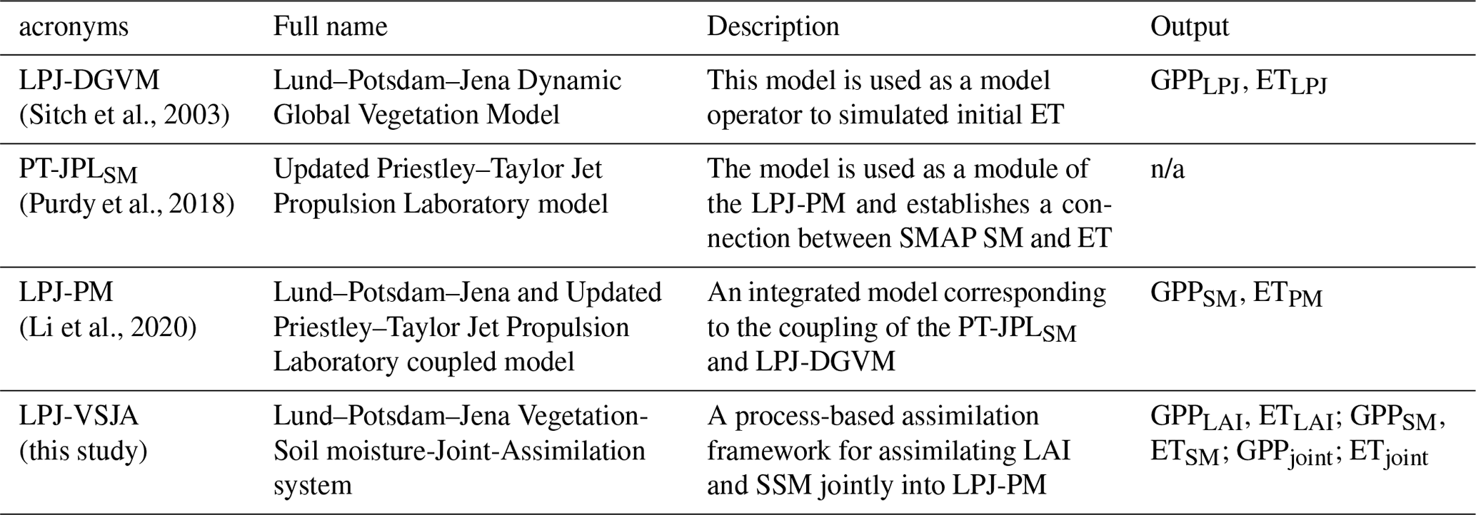
In this study, a coupled terrestrial biosphere model, LPJ-PM, was used to simulate daily GPP and ET by assimilating satellite-derived LAI and SSM. The LPJ-PM is coupled from LPJ-DGVM and PT-JPLSM. The original input data in PT-JPLSM were all inherited from LPJ-DGVM, with the exception of relative humidity (RH) and surface soil moisture (SMOS and SMAP), including the initial LAI calculated by the LPJ-DGVM or assimilated LAI obtained through the LAI assimilation scheme, canopy height, and the fraction of absorbed photosynthetic active radiation (fPAR). The detailed processes of the LPJ-PM have been described in Li et al. (2020), and the flow chart for the coupling is shown in Fig. 1.
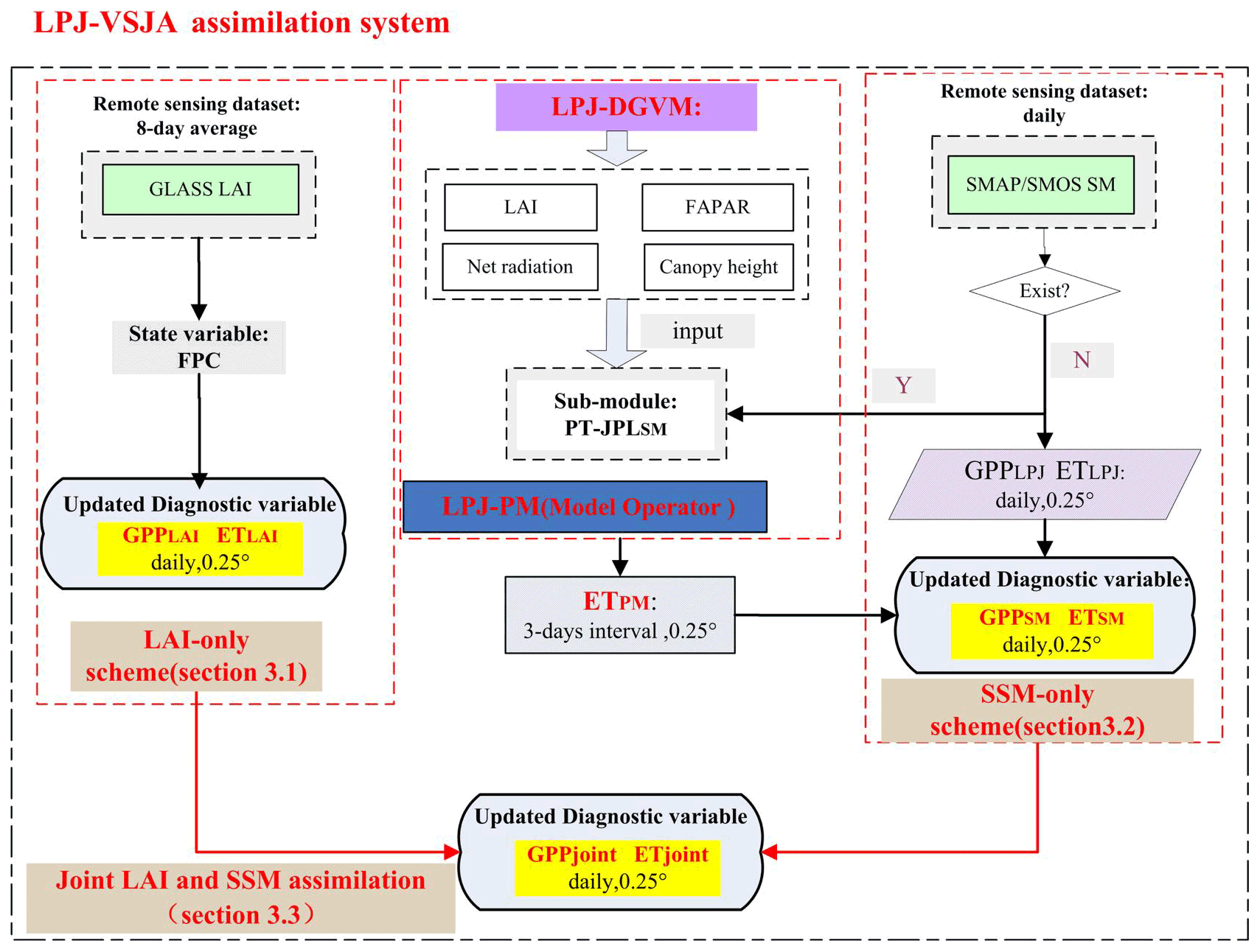
Figure 1Flowchart of the LPJ-VSJA assimilation scheme: three assimilation schemes and the coupled model: LPJ-PM (adapted from Li et al., 2020). The abbreviations in the model and the assimilation framework are explained in Table 1.
2.1.1 LPJ-DGVM
The LPJ-DGVM is a process-oriented dynamic model, which considers mutual interaction of carbon and water cycling and is designed to simulate vegetation distribution and carbon, soil, and atmosphere fluxes (Sitch et al., 2003). For each plant functional type (PFT), the GPP is calculated by implementing coupled photosynthesis and water balance.
The canopy GPP is updated daily:
where JC is the Rubisco limiting rate of photosynthesis, JE is the light-limiting rate of photosynthesis, and the empirical parameter θ represents the common limiting effect between the two terms. JE is related to APAR (absorbed photosynthetic active radiation, product of FPAR and PAR), while JC is related to Vcmax (canopy maximum carboxylation capacity, µmol CO2 m−2 s−1):
where C1 and C2 are determined by a variety of photosynthetic parameters and the intercellular partial pressure of CO2, which is related to atmospheric CO2 content and further altered by leaf stomatal conductance (Sitch et al., 2003). APAR and FPAR are directly related to LAI.
In the water cycle module, ET is calculated as the minimum of a plant- and soil-limited supply function (Esupply) and the atmospheric demand (Edemand) (Haxeltine and Prentice, 1996; Sitch et al., 2003). The soil structure is simplified to a “two-layer bucket” model (the top soil layer at a 0–50 cm depth and the bottom layer at a 50–100 cm depth).
In this module, it is assumed that the soil layer above 20 cm produces water through evaporation, and Wr20 is the relative water content of the soil above 20 cm, which is used as the only soil water limit for calculating vegetation transpiration and soil evaporation. In the evapotranspiration estimation, the oversimplification of soil structure and the soil water limitation lead to a large error (Sitch et al., 2003), while LPJ-DGVM cannot directly assimilate surface soil water due to the limitation of soil layer stratification, and therefore, the satellite-derived SSM cannot be assimilated into LPJ-DGVM directly. The oversimplified soil structure and single soil moisture limitation inevitably lead to sizable uncertainty in ET simulation. Additionally, the monthly input caused a daily variation of the modeled SM, which was also not transmitted to the calculation of GPP and ET. Thus, the updated PT-JPL model (hereafter referred to as PT-JPLSM) was coupled with LPJ-DGVM, and the model structure was modified so that SSM can be directly assimilated into the coupled model at the daily time step.
2.1.2 PT-JPLSM
In PT-JPLSM, three ET components are modeled: soil evaporation (E), vegetation transpiration (T), and leaf evaporation (I). The PT-JPLSM introduced a constraint (0–1, CRSM) of SSM for T and E, which was used to avoid the implicit soil water control (represented by fSM = RHVPD) in the PT-JPL model.
Vegetation transpiration is calculated as follows:
where wobs is the SMAP SSM, wpwp is the water content at the wilting point, and VWC is volumetric water content. wCR is a crucial parameter in characterizing the extent of SM restriction on ET, and wpwp_CH is the canopy height (CH)-adjusted surface soil moisture wilting point and is related to the potential of roots capturing water from deeper sources to limit the transpiration rate and characterize the SM availability (Purdy et al., 2018; Evensen, 2004; Serraj et al., 1999). The specific formula is given in Purdy et al. (2018).
Soil evaporation is calculated as follows:
The proportion of available water limits the soil evapotranspiration to the maximum available water. This scalar was formulated to represent the relatively accurate extractable water content for the vegetation, determined by soil properties and the water available for evaporation, which is estimated via surface water constraints.
The SMAP SSM was applied to model global ET using PT-JPLSM, and the results demonstrated the largest improvements for ET estimates in dry regions (Purdy et al., 2018). Due to the limitation of soil stratification in LPJ-DGVM, the model was coupled with an updated remote sensing ET algorithm in the PT-JPLSM that could better simulate ET in water-limited regions than in humid regions (Purdy et al., 2018).
2.2 Assimilation scheme and experiment procedure
To improve the prediction capability of LPJ-PM, we designed three assimilation schemes: assimilating LAI only (LAI-only, output: ETLAI, GPPLAI), assimilating SSM only (SSM-only, output: GPPSM, ETSM), and joint assimilation of LAI and SSM (Joint LAI and SSM assimilation, output: ETjoint, GPPjoint), i.e., LPJ-VSJA framework) to test the assimilation performance for simulating GPP and ET.
The proposed LPJ-VSJA framework consists of four main components: the model operator (the LPJ-PM), the observation operator (to establish the relation between the assimilation variable and the observed variable), the observation series (GLASS LAI and SMOS or SMAP products), and the assimilation algorithm (POD4DVar). With the surface soil moisture constraint in the PT-JPLSM, the LPJ-VSJA corrects the output fluxes (GPP and ET in this study).
The experiment consisted of six steps.
-
Step 1. Initialize the LPJ-DGVM, and output the reference state variables without assimilation over the experimental period (2010–2018), referred to as the “control run” scenario.
-
Step 2. Implement three assimilation schemes respectively, and the results represent the assimilation integration state (daily GPP and ET assimilation results are referred to as the “GPPLAI” and “ETLAI” in the LAI-only scheme,“GPPSM” and “ETSM” in the SSM-only scheme, and “GPPjoint ” and “ETjoint ” in the Joint LAI and SSM assimilation scheme. This scenario used the same input data and model parameter scheme as the control run scenario.
-
Step 3. Evaluate GPP and ET results (three schemes) by comparing the parameters, R2 ( coefficient of determination), BIAS, and ubRMSD (unbiased root mean square deviation), for conditions of without-DA (control run scenario) and with-DA states, and assess the assimilation performance of separate assimilation and joint assimilation to determine the optimal assimilation scheme for GPP and ET, respectively.
-
Step 4. Evaluate the in situ GPP and ET resulting from the assimilation where the sites are located in wet or dry regions by dividing these validation sites into four parts (humid, sub-dry humid, semi-arid, and arid regions), and this step was designed to assess the superiority of the proposed assimilation scheme in water-limited areas.
-
Step 5. Compare the ET assimilation performance by assimilating the SMOS data with that by assimilating the SMAP data.
-
Step 6. Evaluate the simulated GPP and ET maps based on the optimal assimilation scheme against existing global flux products.
2.2.1 LAI-only assimilation scheme
In the LAI-only assimilation scheme, the observation operator determines the relationship between LAI and foliage projective cover (FPC) in the process model (Eq. 8), and the assimilated LAI will be propagated by energy transmission and ecosystem processes (e.g., photosynthesis, transpiration of vegetative process) in the dynamic model to improve GPP and ET simulations (Bonan et al., 2014; Mu et al., 2007). FPC, the vertically projected percentage of the land covered by foliage, regulates the rate of photosynthate conversion and transpiration. In this study, the GLASS LAI with 8 d interval for the period 2010–2018 was selected as the observation dataset for assimilation, and the FPC state variable was updated daily through running the LPJ-PM (FPCDA, GPPLAI, ETLAI in this study) as shown below:
We set the model and observation errors at a given time as 20 % and 10 % (scale factor) of the LAI value and the observed LAI value, respectively. By verifying the assimilation performance (R2, RMSD, and BIAS) for different scale factors (f) of model simulation and observations in the range of 0.05 to 0.40, taking a step size of 0.05 (a total of 64 combinations), the optimal scale factors (0.2 and 0.1) were determined (Bonan et al., 2020). The model and observation errors was the LAI value multiplied by f. The model integration generation method described by Pipunic et al. (2008) was used to determine the minimum number of ensemble members required to achieve maximum efficiency, and the number of sets was 20.
2.2.2 SSM-only assimilation scheme
In this scheme, the SSM products (SMOS or SMAP) were assimilated into LPJ-PM to obtain more accurate ET (ETSM) estimates in water-limited areas. The observation series was the SMOS or SMAP SSM product, and the observation operator was the PT-JPLSM model. The ETPM (see Table 1) was estimated by the coupled model (LPJ-PM) introducing SSM as a diagnostic variable. The ET values resulting from the assimilation were applied to compute the top layer SM (50 cm) at the next time step (a nonlinear soil water availability function described by Zhao et al., 2013), providing feedback for subsequent hydrologic and carbon cycle processes. Then, the updated SM values regulated the GPP simulation (output: GPPSM). Different from other “constant” ET observations, the ETPM (“observation”) at each time t was adjusted by absorbing intermediate variables updated after assimilation at time t−1. The ETPM was shown to be better than ET simulated by LPJ-DGVM but not as good as that simulated by the model with SMAP SSM assimilated (Li et al., 2020). Thus, it is also proven that this SSM assimilation scheme could improve the accuracy of ET simulations (Li et al., 2020).
Table 1Description of the models and outputs in this study. “n/a” stands for “not applicable”.
All assimilation simulations were conducted between January 2010 and December 2018. Between January 2010 and April 2015, SMOS data were used for assimilation, and after May 2015, both SMOS and SMAP data were used for assimilation. An assimilation scheme was conducted when RH and SMOS or SMAP SSM data existed simultaneously; otherwise, the original simulation of the LPJ-DGVM was conducted directly without adjustment of assimilation.
Similar to the LAI assimilation scheme, the model and observation errors were set as 15 % and 5 % of ETLPJ and ETPM, respectively (LPJ-PM was adopted before assimilation). The number of ensemble members was set to 50. The ETPM must be rescaled to the ETLPJ distribution via their corresponding cumulative probabilities using the cumulative distribution function (CDF) matching to avoid introducing any bias into the LPJ-VSJA system (Li et al., 2020).
2.2.3 Joint LAI and SSM assimilation scheme
In this scheme, both LAI from GLASS and SSM from SMOS or SMAP were the observation datasets. The GLASS LAI was assimilated to obtain the FPCDA and ETLAI, and then the FPCDA served as input to LPJ-PM to simulate optimized ETPM, and the ETjoint was generated using ETLAI and ETPM. Then, the SM (referred to as SMCO in Fig. S1 in the Supplement) updated by ETjoint and the FPCDA were used as input to correct GPP (ETjoint).
Here, we applied the error regulation in the LAI-only scheme and maintained the error setting of the LAI observation and model simulation. Considering the transmission of integrated model error, we recalculated the model error of LPJ-PM after the LAI assimilation and set model and observation errors of ETLAI and ETPM to be 15 % and 10 %, respectively.
2.3 POD-based ensemble 4D variational assimilation method
The proper orthogonal decomposition (POD)-based ensemble four-dimensional variational (4DVar) assimilation method (referred to as PODEn4DVar) (Tian and Feng, 2015) has the advantage of avoiding the calculation of adjoint patterns as its incremental analysis field, which can be represented linearly by the POD base (transformed OP, observing perturbation, and MP, model perturbation). Moreover, the PODEn4DVar can simultaneously assimilate multiple-time observation data and provide flow-dependent (the flow-dependent is the ensembles of forecasting statistical characteristics in the t time) error estimates of the background errors. It has shown advantages in terrestrial assimilation, the Tan-Tracker system (a Chinese carbon cycle data-assimilation system; in Chinese, “Tan” means carbon) and radar assimilation (Tian et al., 2010, 2009, 2014; Zhang and Weng, 2015).
By minimizing the following initial incremental format of the cost function in the 4DVar algorithm, an analysis field can be obtained as follows:
Here, the , , , . is the model perturbation (MP) matrix, and is the observation perturbation (OP) matrix with N samples. Following Rüdiger et al. (2010), the LAI perturbation was set to a fraction (0.001) of the LAI itself. The perturbation of ETPM and ETLPJ conforms to a Gaussian distribution with a mean of 0 and a specified covariance (10 % and 5 % of the ETPM and ETLPJ at time t). The subscript b represents the background field, the superscript T represents a transpose, H is the observation operator of the LAI-only assimilation scheme as described in Sect. 2.2.1, and the SSM-only assimilation scheme is the PT-JPLSM (described in Sect. 2.1.2). M is the forecast model (LPJ-PM in this study), B is the background error covariance, R is the observation error covariance, and obs denotes observation.
Assuming the approximately linear relationship between OP(y′) and MP(x′), POD decomposition and transformation were successively conducted for OP and MP. The transformed OP samples () are orthogonal and independent, and the transformed MP samples () are orthogonal to the corresponding OP samples, where n is the number of POD modes.
The manifestation of the background error covariance is the same as the ensemble Kalman filter (EnKF; Evensen, 2004), and the incremental analysis was expressed by the Φx,n, and . Finally, the optimal analysis xa is calculated as . The detailed derivation process of the algorithm is described by a previous study (Tian et al., 2011).
In the ensemble-based method (Evensen, 2004), the number of ensemble members is usually fewer than that of the observation data and the degrees of freedom of the model variables, and spurious long-range correlations occur between observation locations and model variables. A practical method, the localization technique, is applied to address this issue (Mitchell et al., 2002). The final incremental analysis is rewritten as
where dh and dv are the horizontal and vertical distances between the spatial positions of state and observed variables, respectively; and dh,0 and dv,0 are the horizontal and vertical covariance localization Schur radii, respectively. The filtering function C0 is expressed as
where r is the radius of the filter.
The assimilation algorithm is mainly divided into two steps: (1) prediction, by running LPJ-PM in the current assimilation window and generating simulation results and background field vectors, and (2) update, the algorithm being used to calculate the optimal assimilation increment and analysis solution xa. The simulation results and the initial conditions of the model in the current window are updated using the analysis solution. The updated initial conditions were applied for model LPJ-PM prediction, and the above process was repeated.
2.4 Validation method for assimilation performance
The R2 (coefficient of determination), BIAS, and ubRMSD (unbiased root mean square deviation) between simulation and tower-based observations were applied for evaluation. In addition, a Taylor chart was also used to demonstrate the performance of two ET estimations with different SSM observations in terms of R, ubRMSD, and normalized standard deviation (NSD) on 2D plots, to display how closely the datasets matched observations in one diagram (Taylor, 2001). In the Taylor diagram, NSD represents the radial distance from the origin point and the correlation with the site observations as an angle in the polar plot. The ubRMSD is the distance between the observation and the model and is represented in the Taylor chart as a green semi-circular arc with point A as the center of the circle. The closer the model point to the reference point (Point A), the better the performance. This diagram is convenient and visual in evaluating multiple aspects of various models.
The error variance of GPP and ET products was estimated using the triple collocation (TC) approach (Stoffelen, 1998) to validate the global simulation in this study. The method has been extensively applied in the study of hydrology and oceanography (Caires and Sterl, 2003; Khan et al., 2018; O'Carroll et al., 2008; Stoffelen, 1998), particularly in SM studies (Chan et al., 2016; Kim et al., 2018). The TC provides a reliable platform for comparison of spatial assimilation results and in situ measurements. In this experiment, no calculation was performed on the non-vegetated areas, where the correlation was lower than 0.2, in order to have independent datasets and avoid correlated errors (crucial assumptions in TC) (Yilmaz and Crow, 2014).
In this study, the five products were divided into three product categories, including satellite products (MODIS and GOSIF GPP), reanalysis products (GLASS and GLDAS), and data-assimilation products (GLEAM ET and LPJ-VSJA) (C. Li et al., 2018). One product in each category was selected to form a group to calculate their error. The LPJ-VSJA product was set as the reference data.
For GPP products, GOSIF, GLASS, and LPJ-VSJA were treated as a group, and MODIS, GLASS and LPJ-VSJA were treated as another group to calculate the errors; the final errors were determined by the average of these two.
Similarly, to calculate the errors for ET, GLEAM, GLASS, and MODIS were chosen as a group; LPJ-VSJA, GLDAS, and MODIS were treated as a group; LPJ-VSJA, GLASS, and MODIS were considered a group. In order to reduce the influence of orthogonality hypothesis of error, the first and third groups are for indirect and effective comparison between LPJ-VSJA product and GLEAM product.
3.1 Description of flux tower sites
We screened over 300 eddy covariance (EC) flux sites across the globe from the FLUXNET2015 (https://fluxnet.org/data/fluxnet2015 dataset/, last access: 10 April 2021), AmeriFlux (https://ameriflux.lbl.gov/data-and-manifest/, last access: 10 April 2021), and the HeiHe River basin (https://doi.org/10.11888/Hydro.tpdc.270888, Xie, 2017) for the evaluation of assimilation performance over the period from January 2010 to December 2018. The in situ half-hourly latent heat flux (LE) and GPP data from the sites were aggregated into daily data. The daily gap-filled data were excluded if the percentage of gap-filled half-hourly values was more than 20 %. Then we corrected the data of energy non-closure using the Bowen ratio closure method (Twine et al., 2000) to improve the energy closure rate (Huang et al., 2015; Yang et al., 2020). The data were selected to cover the 2010–2018 period with at least 1 year of reliable data, and the result from the error of assimilation is relative to the LE value and seasonal variation (Purdy et al., 2018; Zou et al., 2017). It is essential to have available data every month during a 1-year period, and only days with less than 25 % missing data were processed per month (Feng et al., 2015). In addition, for flux tower data, the data were also excluded for the analysis if the SMAP/SMOS SSM data were not of good quality.
Finally, we identified a total of 105 sites across the globe encompassing five major biomes: grassland (18 for GPP and 19 for ET), savanna (11), shrubland (4), forest (49 and 53), and cropland (13 and 14). In the comparative analysis of the performance for simulating ET by assimilating SMOS and SMAP SSM data separately, we selected 46 AmeriFlux sites (Fig. S3) with at least 1 year of reliable data from 2015 to 2018 based on the simultaneous availability of SMAP and SMOS data, including grassland (19), savanna (11), shrubland (5), forest (23), and cropland (7). Figures S2 and S3 illustrate the location and distribution of the 105 and 46 EC flux tower sites, respectively. A more detailed description is summarized in Table S1 in the Supplement.
3.2 Remote sensing datasets: LAI and SSM
The GLASS LAI product with an 8 d time step (8 d average) and 5 km resolution was derived from MODIS and CYCLOPES surface reflectance and ground observations using general regression neural networks (GRNNs) (Xiao et al., 2013, 2016). The verification of the product using the mean values of high-resolution LAI maps showed that the GLASS LAI values were closer to these high-resolution LAI maps (RMSD = 0.78 and R2 = 0.81) (Xiao et al., 2016; Liang et al., 2013). Therefore, the GLASS LAI product has satisfactory performance and can be assimilated into terrestrial biosphere models.
The SMAP mission (Entekhabi et al., 2010) and SMOS mission (Jacquette et al., 2010), the two dedicated soil moisture satellites currently in orbit equipped with L-band microwave instruments, provide SSM retrievals. We chose the SMOS-L2 product and the SMAP-L3-Enhanced product, which both provide global coverage every 3 d for soil depth of 5 cm. Only good-quality SMAP and SMOS data were used. The grid cells with water areas larger than 10 % and those with less than 50 % good-quality data in 1 year were masked out, which alleviates the undesirable model simulations caused by the decrease in SMAP retrieval accuracy (Chan et al., 2016; O'Neill et al., 2010). We only adopted the data with an uncertainty below 0.1 m3 m−3, in the actual range (0.00–0.6 m3 m−3), and the temperature of the Land Surface Module (LSM) observation layer (the second layer) was higher than 2 ∘C (Blyverket et al., 2019).
The GLASS LAI, SMOS, and SMAP observations were resampled to 9 km for site simulation and 0.25∘ for regional simulation. The 8 d average of GLASS LAI was assimilated for each day, and the SMAP or SMOS SSM was assimilated every 3 d.
3.3 Model-forcing and validation datasets
In this study, the meteorological, soil property, and CO2 concentration datasets were used to drive the LPJ-PM. The climate-driven datasets used for the initialization of the LPJ-DGVM are the atmospheric CO2 concentrations (1901–2018) of ice-core measurements and atmospheric observations at the Mauna Loa Observatory and CRU TS4.03 version Climate data from 1901 to 1930 provided by the Climatic Research Unit (CRU) of the Climate Laboratory, University of East Anglia, UK, including monthly precipitation, surface temperature, cloud cover and wet day. In the simulation period of 2010–2018, the Modern Era Retrospective-Analysis for Research and Applications Version 2 (MERRA-2) was adopted, and the variables used included precipitation, temperature, cloud cover, and relative humidity. Soil properties (including limited water content of vegetation at wilting points, field capacity, and soil porosity) from the Harmonized World Soil Database (HWSD) V1.2 dataset (Wieder et al., 2014) were selected as inputs to the PT-JPLSM model. Table 2 provides the spatial and temporal characteristics of the model-forcing datasets in the LPJ-PM (submodule: LPJ-DGVM and PT-JPLSM).
Table 2List of the selected forcing and remote sensing datasets used in this study.
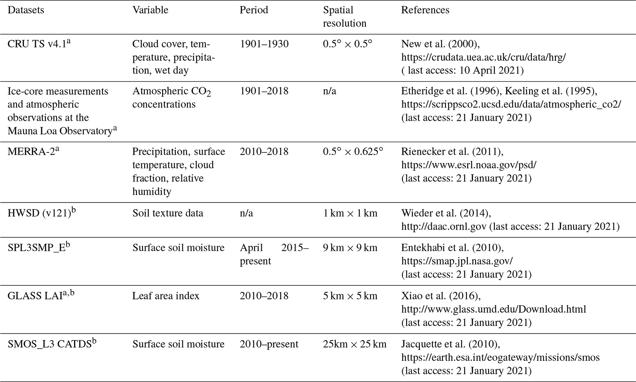
a Forcing dataset for LPJ-DGVM. b External input dataset for PT-JPLSM.
The GLASS LAI product, SMOS-L2 product, and the SMAP-L3-Enhanced product were assimilated to simulate GPP and ET. For site simulation, in order to maintain consistency with the SMAP Enhanced 3 Level product (Entekhabi et al., 2010), model-forcing data were resampled to a 9 km spatial resolution based on EASE-2 projection grid. In the global spatial simulation, the model-forcing datasets were resampled to 0.25∘ based on the bilinear method to ensure the consistency of spatial representation.
Table 3Global GPP and ET products for comparison in this study.
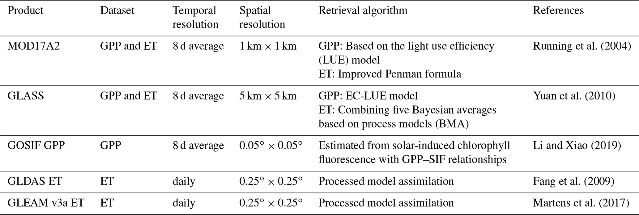
We used four global ET products and three global GPP products (S. Li et al., 2018; Li and Xiao, 2019; Wang et al., 2017) that was resampled to 0.25∘ to evaluate the performance of the model with the joint assimilation scheme. Table 3 shows the details of these GPP and ET products.
4.1 Performance of LPJ-PM for simulating GPP and ET with the assimilation of LAI and soil moisture
4.1.1 Accuracy assessment of GPP for separate and joint assimilation
In general, the R2 between GPPLPJ and GPPOBS was above 0.4 at most of the sites (62 sites) and was relatively weak for some sites. The LAI assimilation improved the simulations at most sites (R2 value increased at 82 sites), particularly for sites in the United States and Europe (Fig. S4). The R2 improvement from the LAI assimilation (LAI-only assimilation) was superior to that from the SSM assimilation (Fig. S4b and c). The performance of the joint assimilation was similar to that of LAI-only assimilation. Sites (Fig. S5a) that showed positive BIAS (GPPOBS–GPPLPJ) were mainly distributed in the humid and sub-dry humid forest, grassland, and arid cropland regions, showing underestimation for GPPOBS. The assimilation improved the accuracy for overestimated sites, but there was no significant improvement for underestimated sites. The ubRMSD implied that the SSM assimilation alone had a better performance than the LAI assimilation alone, especially for sites in arid areas (Fig. 2). The analysis of the above three statistical measures (R2, BIAS, and ubRMSD) indicated that the accuracy of joint assimilation was much better than that of each separate assimilation.
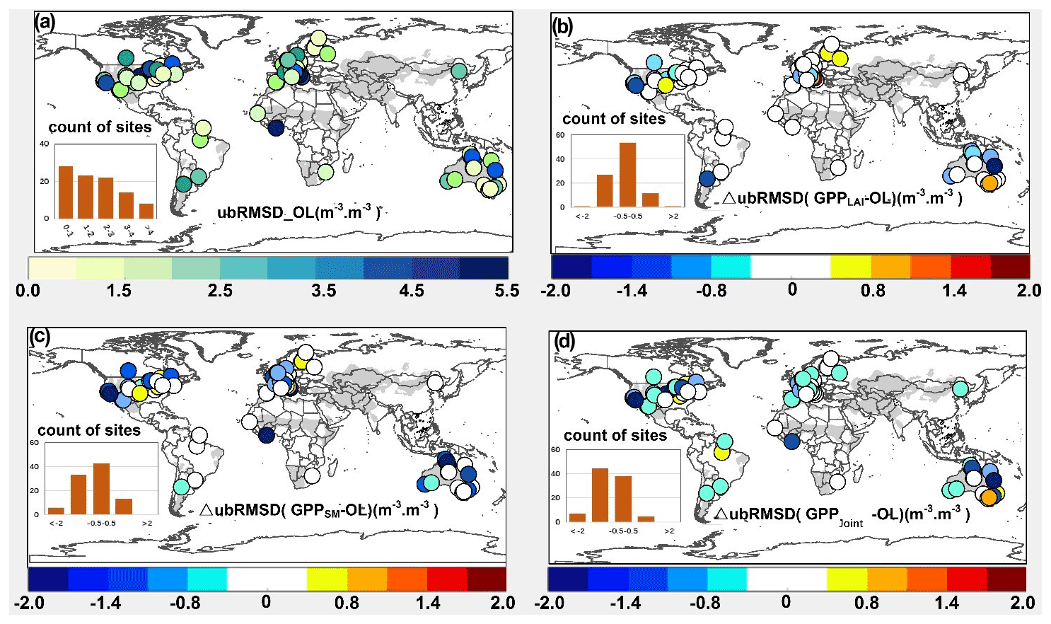
Figure 2(a) The unbiased root mean square error (ubRMSD) between the GPPLPJ and the site observations, with yellow/blue indicating low/high ubRMSD. (b) ΔubRMSD (GPPLAI–GPPLPJ). (c) ΔubRMSD (GPPSM–GPPLPJ). (d) ΔubRMSD (GPPJoint–GPPLPJ). Blue/red represents positive/negative values.
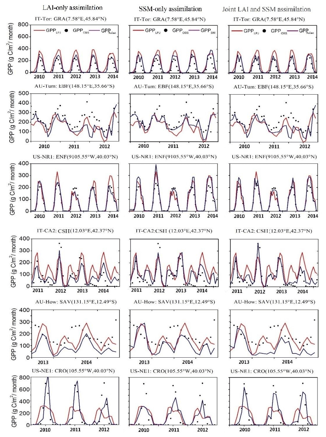
Figure 3Seasonal cycles of tower GPP and simulated gross primary productivity (GPP) from Lund–Potsdam–Jena (LPJ), LAI-only assimilation, SSM-only assimilation, and joint assimilation for six sites representing six PFTs.
At the seasonal scale, all three assimilation schemes corrected the model trajectory and significantly improved the growing season simulations, especially for peak values (IT-Tor, US-NR1, and US-NE1) (Fig. 3). In addition, the linear fitting of GPPjoint and GPPOBS on a monthly scale was closer to 1 : 1 (, p < 0.001) than that of GPPLAI (, p < 0.001) and GPPSM (, p < 0.001) (Fig. S9). The results in Table S2 support the above analysis, and the joint assimilation showed advantages in overall accuracy in both arid and humid areas.
The residual analysis indicated that the three assimilation schemes for GPP (Fig. S11 left) were different. For the assimilation results, most of the errors were distributed around −70–60 g C m−2 per month. The high GPPOBS values were considerably underestimated. The maximum negative error reached 100 g C m−2 per month. The error distribution of GPPSM was more dispersed than that of GPPLAI and GPPjoint. Among the residuals of these three schemes, GPPSM significantly overestimated the GPPOBS, mainly distributed in the 0–200 g C m−2 per month range. GPPLAI showed significant improvement in the overestimation of GPPOBS compared with GPPjoint. In general, the GPPjoint with the most concentrated error distribution had significant improvement.
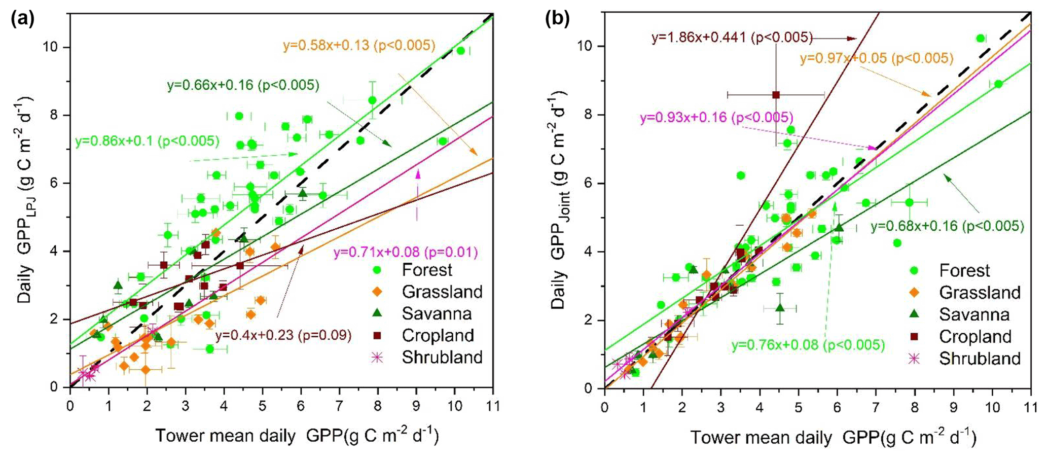
Figure 4Scatter plots of daily GPPLPJ (a) and GPPjoint (b) versus tower GPP for different PFTs.
After determining the optimal assimilation scheme (Joint LAI and SSM assimilation scheme), we evaluated the GPPLPJ and GPPjoint at the site level (Fig. 4). The results showed that GPPjoint performed better (R2 = 0.83, ubRMSD = 1.15 g C m−2 d−1) than GPPLPJ (R2 = 0.69, ubRMSD = 1.91 g C m−2 d−1). The noticeable underestimation in all PFTs and overestimation at most forest sites for GPPLPJ were corrected by joint assimilation (GPPjoint). Our joint assimilation methods had better performance in forests, shrublands, and grasslands than in croplands and savannas. Except for the cropland, the linear fitting results of other types were all below the 1 : 1 line, showing the overall underestimation. Superior performance in both the original simulation and assimilation occurred at shrubland (R2 = 0.93, ubRMSD = 0.89 g C m−2 d−1) and grassland (R2 = 0.97, ubRMSD = 0.83 g C m−2 d−1) sites. However, the standard deviation of GPPjoint and GPPOBS at savanna sites was relatively large, and the GPPjoint at several savanna sites was significantly underestimated.
4.1.2 Accuracy assessment of ET for separate and joint assimilation
In general, the coefficient of determination (R2) between ETLPJ and ETOBS was generally over 0.4 (the simulations were superior to GPPLPJ) (Fig. S6). ETLAI showed slightly higher R2, while some sites showed reduced values (41 sites). The ETSM and ETjoint were significantly improved compared with the ETLAI. The R2 increased considerably in Australia but declined at some sites in the United States after assimilation. For ubRMSD, ETjoint performed better than ETSM and ETLAI. The SSM assimilation improved more in humid regions, while the ubRMSD of ETSM was slightly higher in South America (Fig. 5). In the original LPJ-DGVM simulation, the sites with a negative BIAS were mostly located in the humid and sub-dry humid regions, while most of the sites in arid and semi-arid regions had underestimation (Fig. S7a, Table S3). The assimilation improved ET at some of the overestimated sites, but the underestimation over these sites showed little improvement.
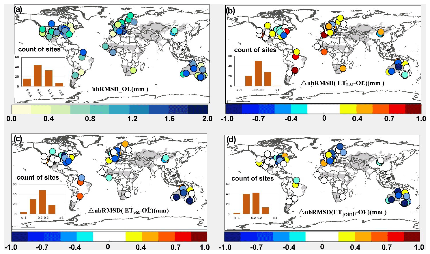
Figure 5(a) The unbiased root mean square error (ubRMSE) between the ET simulated by the LPJ-DGVM and the site observations, with yellow/blue indicating low/high ubRMSD. (b) ΔubRMSD (ETLAI–ETLPJ). (c) ΔubRMSD (ETSM–ETLPJ). (d) ΔubRMSD (ETJoint–ETLPJ). Blue/red represents positive/negative values.
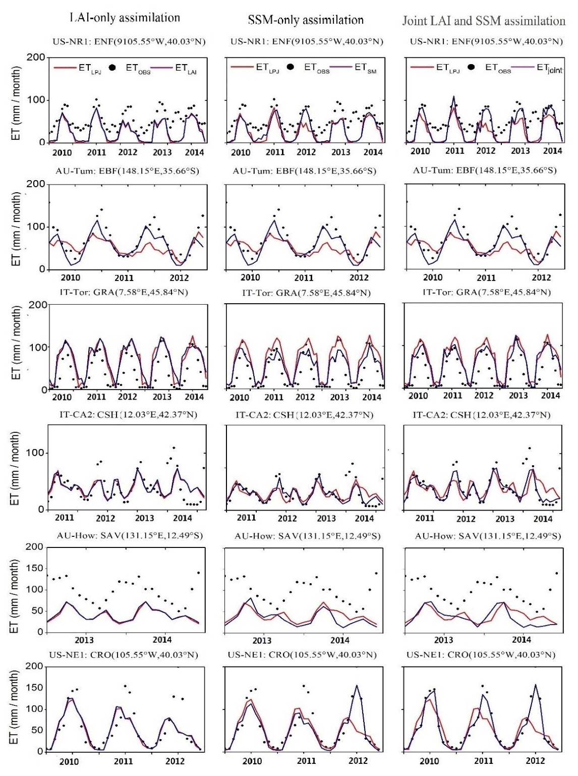
Figure 6Seasonal cycles of tower-based and simulated ET from Lund–Potsdam–Jena (LPJ), LAI-only assimilation, SSM-only assimilation, and joint assimilation for the six sites representing six PFTs during the study period.
At the seasonal scale, the model simulations were able to capture the temporal trend of ETOBS, and joint assimilation significantly improved the simulation in the growing season (US-NR1, US-NE1); overall underestimation was observed for ETOBS, especially in winter (Fig. 6). Overall, the linear fitting of monthly ETjoint and ETOBS was closer to 1 : 1 than that of ETLAI and ETSM (Fig. S6). The simulation accuracy of joint assimilation was better than that of each separate assimilation, and the performance of the SSM assimilation was better than that of the LAI assimilation.
The ET residual analysis (Fig. S11 right) indicated that the three assimilation scheme errors showed underestimation for ETOBS. In general, the error distribution of separate assimilations was more dispersed than that of the joint assimilation. Similar to the assimilation performance of GPP, ETjoint and ETSM significantly improved the overestimation of ETOBS but did not significantly improve the underestimation. For the ETjoint, most of the errors were distributed around −30–18 mm per month. The region with high ETOBS was considerably underestimated, and the maximum negative error reached −57 mm per month.
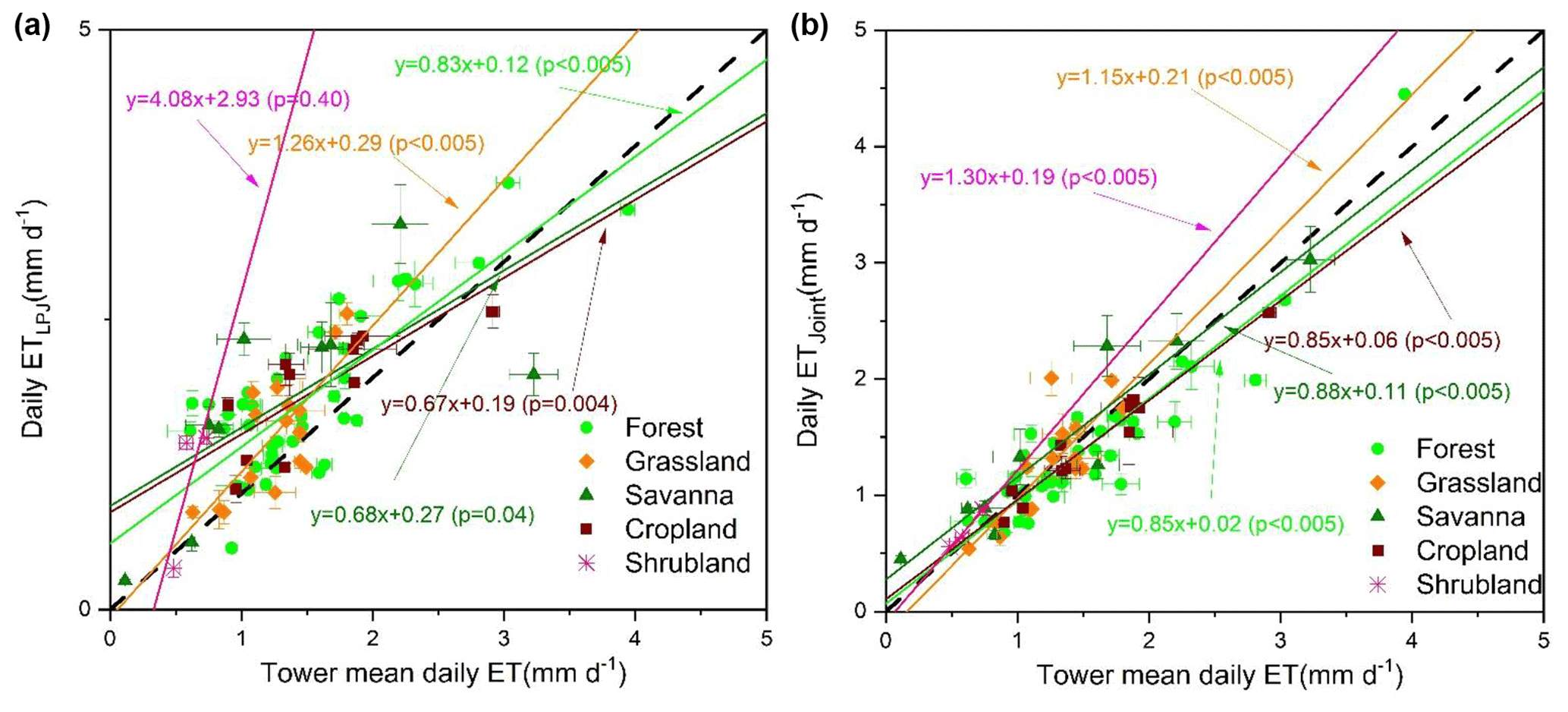
Figure 7Scatter plots of daily ETLPJ (a) and daily ETjoint (b) versus tower ET for different PFTs.
We also evaluated the ET assimilation results at the PFT scale (Fig. 7). The results showed that our ET values resulting from the assimilation performed better at the site level (R2 = 0.77, ubRMSD = 0.65 mm d−1) than that of ETLPJ (R2 = 0.67, ubRMSD = 0.95 mm d−1). Joint assimilation significantly reduced the errors of those shrubland sites with overestimation for ETOBS, and the site distribution was closer to the 1 : 1 line. Our assimilation methods had better performance in forest, savanna, and grassland ecosystems than in cropland and shrubland (Table S3). The linear fitting results of grassland and shrubland were all above the 1 : 1 line, showing overall overestimation. Although the original simulation and assimilation performance were superior at savanna sites (R2 = 0.95, ubRMSD = 0.78 mm d−1), the standard deviations of ETjoint and ETOBS at savanna sites were relatively large, which was similar to the GPP results at savanna sites.
4.2 Comparison of assimilation performance in semi-arid and arid regions with that in humid and sub-dry humid regions
During the period 2010–2014, monthly GPPjoint and ETjoint performed differently in humid and sub-dry humid regions and semi-arid and arid regions (Fig. 8, Tables S2, S3). Overall, the GPP and ET simulations had good consistency with the tower data in the two regions. For GPPjoint, there was no significant difference in the correlation and fitting coefficients between the two regions. As for ETjoint, the fitting results and R2 values in the semi-arid and arid regions performed better than those in the humid and sub-dry humid regions, which also suggested the importance of SSM for ET estimation in water-limited areas.
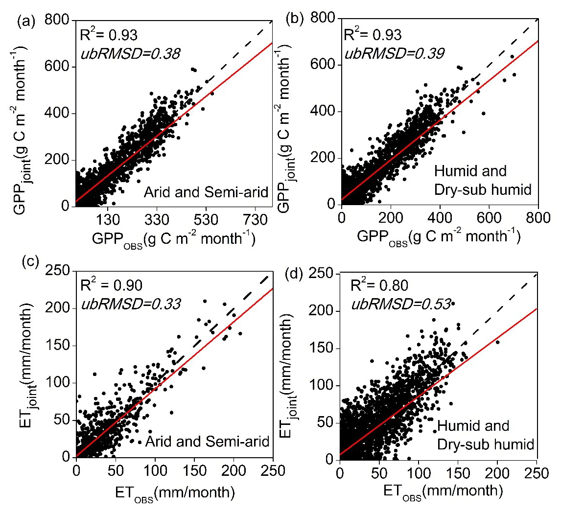
Figure 8Scatter plots of daily tower GPP and ET versus GPPjoint and ETjoint under arid and humid sites: (a, c) the fitting results of GPP and ET in arid and semi-arid regions, respectively, and (b, d) the fitting results of GPP and ET in humid and dry sub-humid zone, respectively.
On the daily scale, the original GPP simulations (GPPLPJ) performed better in the semi-arid and arid regions than in the humid and sub-dry humid regions with higher R2 and lower ubRMSD (Table S2).
The R2 and BIAS implied that the LAI assimilation alone had a better performance than the SSM assimilation alone. However, for sites in arid and semi-arid areas, the ubRMSD showed that the GPPSM improved better than GPPLAI, which both demonstrated SSM data are essential in water-limited regions. For GPPjoint, the shrubland in the semi-arid and arid regions had the lowest R2 values and the second lowest ubRMSD. The forest in the semi-arid and arid regions had the largest improvement after assimilation. In the humid and sub-dry humid regions, the GPPjoint of the savanna and cropland showed the largest improvement (R2 increased by 64.7 % and 71.1 %, respectively; ubRMSD decreased by 47.0 % and 31.8 %, respectively). The grassland in the semi-arid and arid regions had the highest R2, and the savanna by combining all indicators had the best assimilation results compared to other types in both regions.
Similar to ETjoint (Table S3), the ETLPJ in the semi-arid and arid regions was better than that in humid and sub-dry humid regions in terms of four evaluation indicators (ubRMSD decreased by 34.4 % in semi-arid and arid regions and the ubRMSD decreased by 30.9 % in humid and sub-dry humid regions compared with ETLPJ). The R2 and ubRMSD implied that the SSM assimilation alone had a better performance than the LAI assimilation alone, especially for sites in arid areas. and the BIAS showed that the ETLAI improved better than ETSM for sites in humid and sub-dry humid areas. The performance of the original simulation and assimilation of grassland sites in the semi-arid and arid regions was the best among all five PFTs.
To investigate the reasons for better assimilation performance in water-limited regions, we evaluated the GPP and ET simulated by the LPJ-PM according to R2, ubRMSD, and BIAS (Fig. 9). Compared with the semi-arid and arid regions, the humid and sub-dry humid region had smaller R2 mean, larger BIAS, and no significant difference in mean ubRMSD for GPPSM. In general, the evaluation results of joint assimilation for ETPM were generally consistent with those for GPPSM and GPPSM. ETPM showed underestimation, which was consistent with the underestimation in SSM assimilation. These results indicated that both GPP and ET modeled by LPJ-PM with joint assimilation were less stable and had a lower performance in the humid and sub-dry regions than in the semi-arid and arid regions.
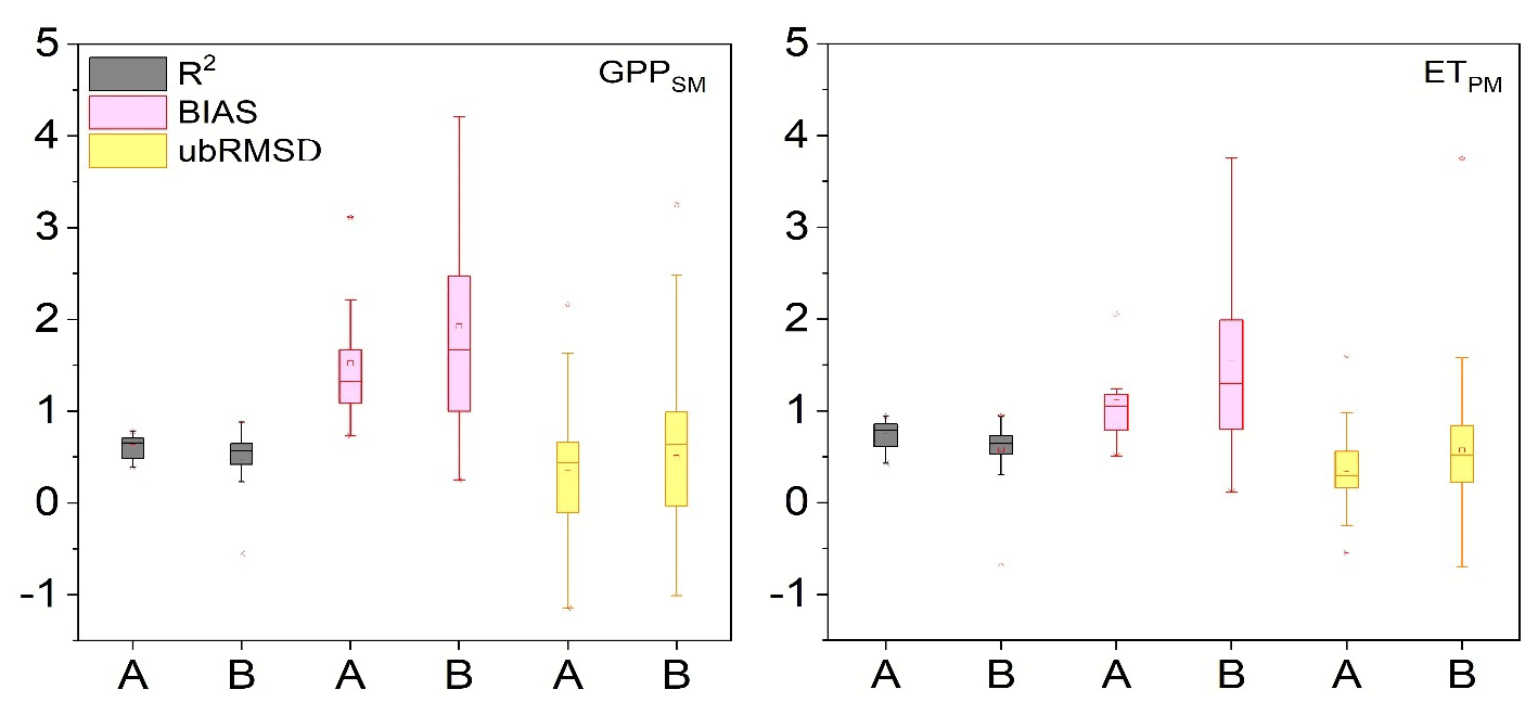
Figure 9Box plots of R2, ubRMSD, and BIAS for GPPSM (a) and ETPM (b). A represents the sites in arid and semi-arid areas, and B represents the sites in humid and dry sub-humid areas.
4.3 Comparison of assimilation performance in assimilating SMOS and SMAP soil moisture data
The Taylor chart was used to compare the assimilation performance of ETSMAP and ETSMOS at 46 AmeriFlux sites (Fig. 10 left). The results showed that ETSMAP performed better than ETSMOS for most PFTs, except forest. Both ETSMAP and ETSMOS performed well for grassland (closer to point A), and there was little difference between R2 and ubRMSD. The NSD of ETSMAP in grassland was 0.88, which was closer to 1 than that of ETSMOS. The assimilation of ET had a lower R2 and higher ubRMSD (0.7–0.8) in forest than other PFTs, and the NSD of cropland and shrubland was lower than that of other PFTs (0.6–0.8), indicating that the assimilation for cropland and shrubland could not reproduce the variations in ET effectively. However, ETSMAP showed significant improvement in R2 compared with ETSMOS for shrubland and cropland. The assimilation performance of ETSMAP and ETSMOS for savanna showed the greatest difference. In general, the ETSMAP and ETSMOS were slightly different, and the ETSMAP was more improved than ETSMOS.
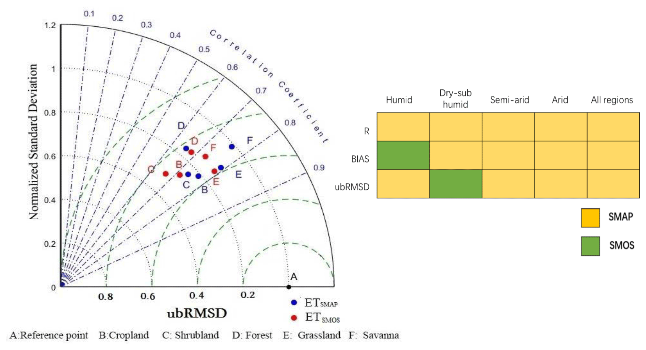
Figure 10Taylor diagram (left) comparing ET simulations with observations at all 46 AmeriFlux sites at the daily time step between April 2015 and December 2018. Blue dots represent results based on assimilation with SMAP SSM only, and red dots represent results based on assimilation with SMOS SSM only. Reference points A and B–F correspond to the vegetation functional types (PFTs). The grid diagram (right) compares the evaluation indices of ET simulations with those of the observed values at all 46 AmeriFlux sites with different wet and dry zones at the daily time step; the yellow cells indicate that ETSMAP performs better in the metric, and green cells indicate that ETSMOS performs better in the metric.
Figure 10 (right) shows the assimilation accuracy of ETSMOS and ETSMAP in different humid and arid regions. The ETSMAP had significant advantages for the four indicators. The R2 of ETSMAP was higher than that of ETSMOS in all the areas. However, ETSMOS in some evaluation indicators showed a better performance than ETSMAP (BIAS in the humid region; ubRMSD in the sub-dry humid region). This may be due to the overall more humid nature of SMOS SSM than the SMAP SSM. Moreover, the sensitivity of deep soil moisture contributed more to the ET in humid areas than in the water-limited areas.
4.4 Global simulations of GPP and ET with joint assimilation of LAI and soil moisture data
To assess the spatial scalability of the LPJ-VSJA assimilation scheme, we simulated the global daily GPP and ET for 2010–2018 with a spatial resolution of 0.25∘. The original results simulated by the LPJ-DGVM and LPJ-VSJA were referred to as LPJ-DGVM GPP(ET) and LPJ-VSJA GPP(ET), respectively. We compared the annual spatial GPP and ET values and the error standard deviation of the LPJ-VSJA with several existing flux products.
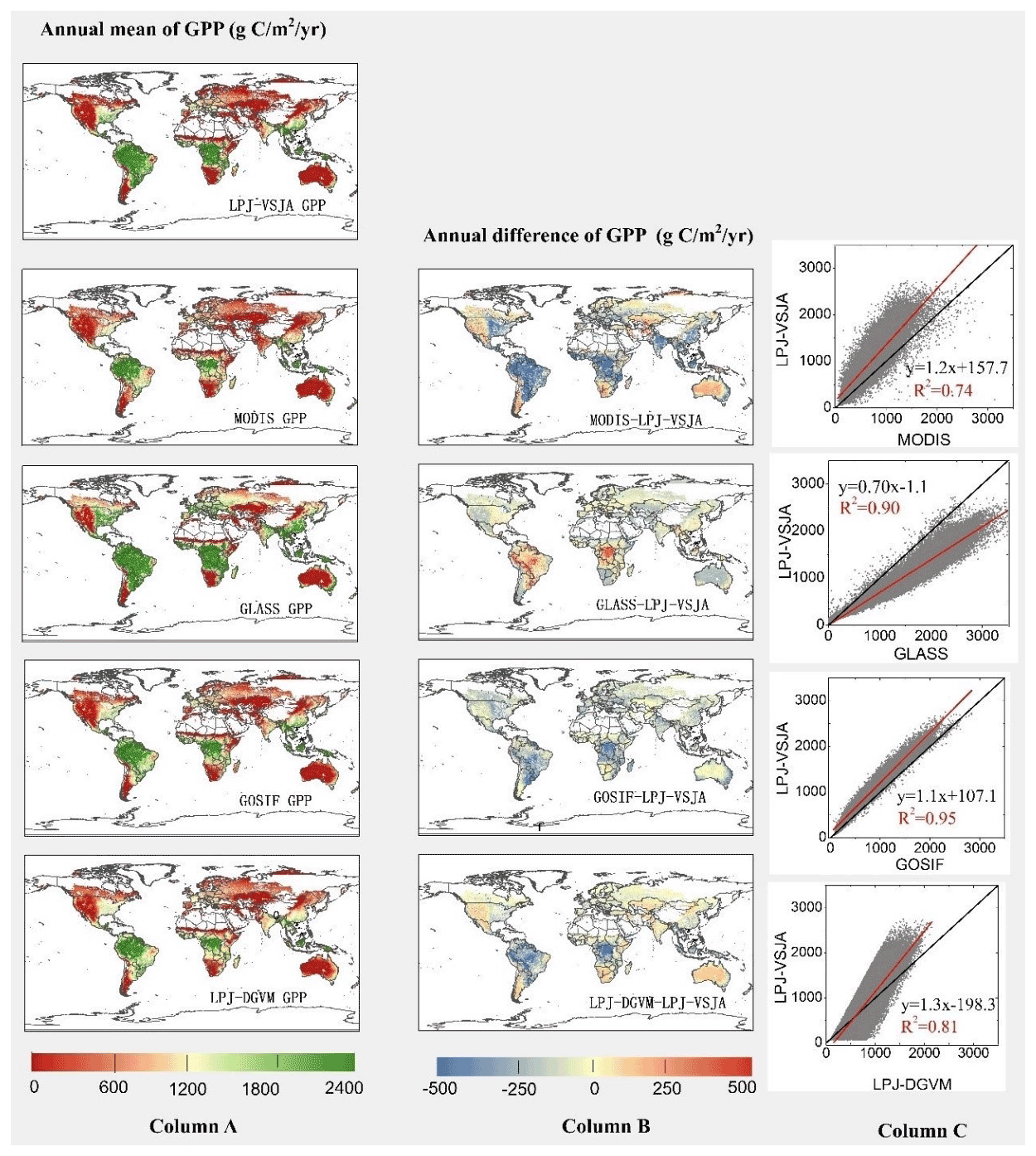
Figure 11Column A: spatial distribution of annual LPJ-VSJA GPP and other independent satellite-based datasets. Column B: spatial distribution of the difference between annual LPJ-VSJA GPP and other independent satellite-based datasets. Column C: scatter plots between these products. Black lines show the 1 : 1 line, and red lines show the regression fit.
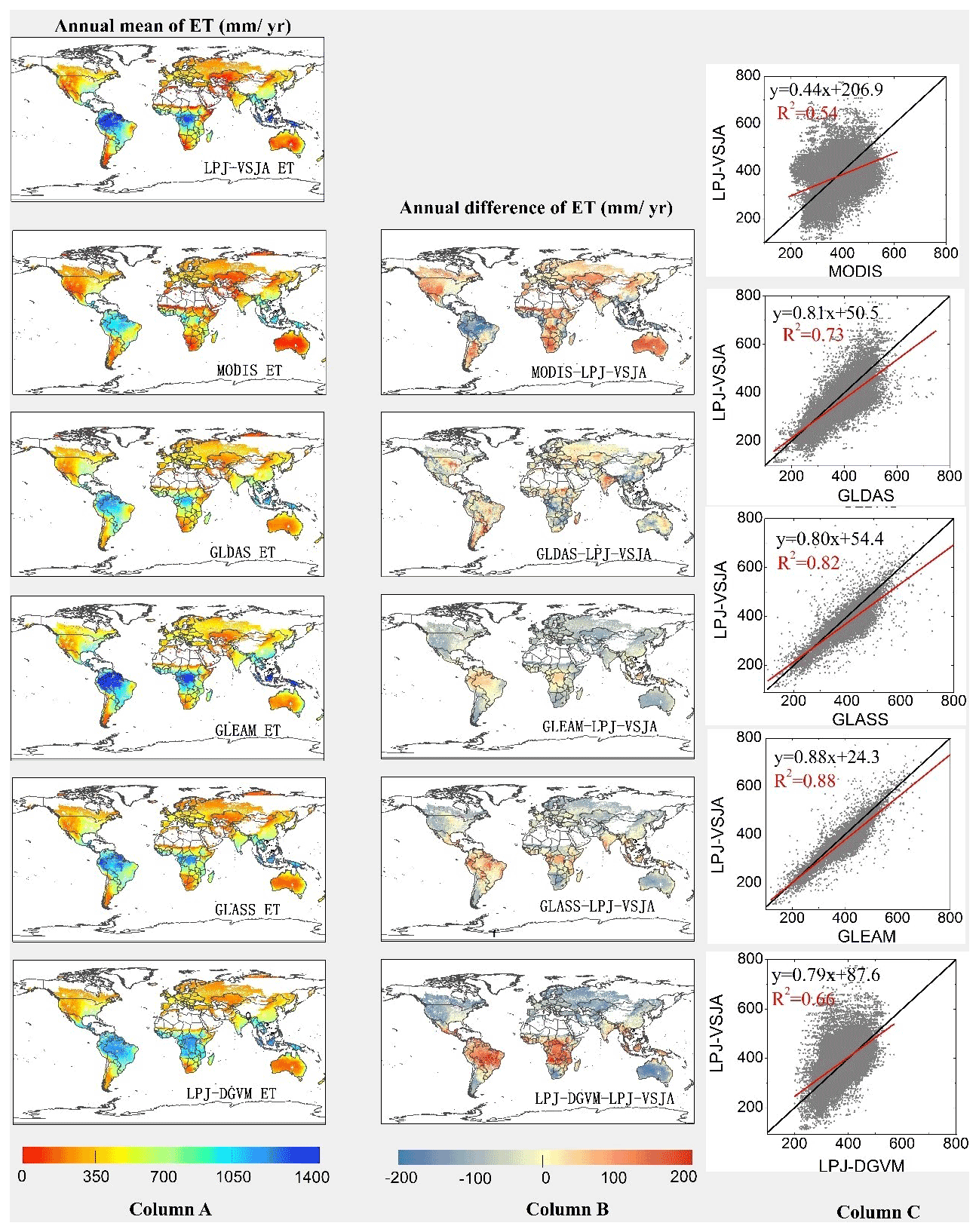
Figure 12Column A: spatial distribution of annual LPJ-VSJA ET and other independent satellite-based datasets. Column B: spatial distribution of the difference between annual LPJ-VSJA ET and other independent satellite-based datasets. Column C: scatter plots between these products are provided on the right of the difference maps. Black lines show the 1 : 1 line, and red lines show the regression fit.
Figures 11 and 12 depict the spatial distribution of the annual mean and the differences between our simulation results and the global independent satellite-based products. The developed LPJ-VSJA GPP was the closest to GOSIF GPP (Li and Xiao, 2019) in most regions with the lowest spatial mean deviation (LPJ-VSJA-GOSIF) (27.9 g C m−2 yr−1), followed by GLASS GPP (51.2 g C m−2 yr−1) (Yuan et al., 2010), LPJ-DGVM (−73.4 g C m−2 yr−1), and MODIS GPP (93.1 g C m−2 yr−1). LPJ-VSJA had higher GPP values than GOSIF GPP in tropical regions, such as Amazonia, Central Africa, and Southeast Asia. In general, the annual mean and differences between MODIS, GOSIF GPP, LPJ-DGVM, and our LPJ-VSJA were in broad agreement (with higher R2 ranging from 0.74 to 0.95).
LPJ-VSJA ET was the closest to GLEAM ET on the spatial average with the least spatial average deviation (−13.9 mm yr−1) and highest R2 (0.88), followed by GLASS ET (−23.1 mm yr−1 and 0.82), GLDAS ET (−34.7 mm yr−1 and 0.73), LPJ-DGVM (−48.7 and 0.66 mm yr−1), and MODIS ET (−122.1 and 0.54 mm yr−1).
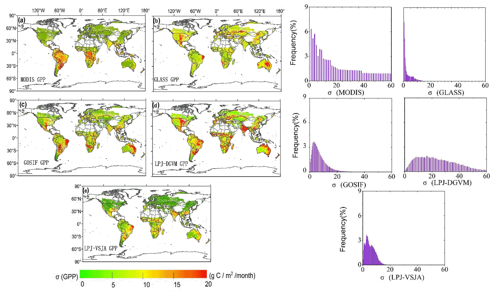
Figure 13Spatial distribution and histograms of error standard deviation (σ) for global GPP products: MODIS (a), GOSIF (b), GLASS (c), LPJ-DGVM (d), and LPJ-VSJA (e).
Figure 13a–e represent the spatial error standard deviation (σ) distribution of MODIS, GLASS, GOSIF, and LPJ-VSJA GPP, respectively. The graphs on the right side depict the corresponding histograms. The σ of the MODIS GPP was evenly distributed between 30 and 60 g C m−2 per month, while the average σ of other products was concentrated in 0–20 g C m−2 per month (90 %). The high errors of all products were concentrated in the hot and humid areas of southern North America, eastern South America, humid and dry sub-humid areas of South Asia, and the savannas of Africa and Australia. The error histogram of GOSIF GPP and LPJ-DGVM GPP was in line with the normal distribution, with an average value of 8.3 and 22.4 g C m−2 per month. The GLASS GPP product had the lowest mean value (3.6 g C m−2 per month), followed by LPJ-VSJA (4.7 g C m−2 per month), but the error variance of the LPJ-VSJA product was the lowest, indicating the stability of the regional error (Table S4). Compared to the LPJ-DGVM, the joint assimilation results showed improvement in all regions (the average error reduced by 17.7 g C m−2 per month), especially in the humid regions of South Asia, Australia, and the United States. Our LPJ-VSJA GPP was generally proven to have high accuracy and stability for spatial analysis and could provide a reference for other model products.
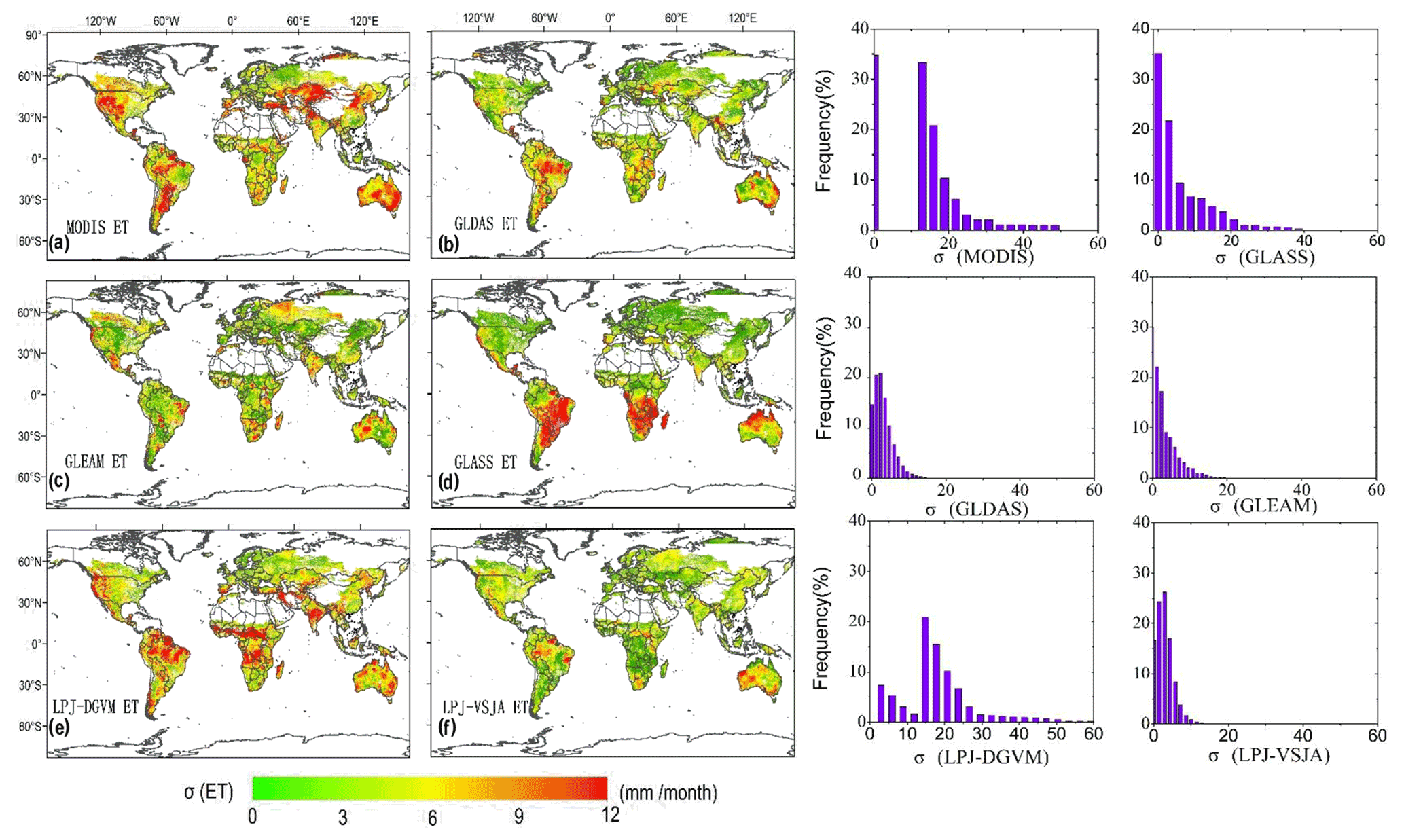
Figure 14Spatial distribution and histograms of error standard deviation (σ) for global ET products: MODIS (a), GLDAS (b), GLEAM (c), GLASS (d), LPJ-DGVM (e), and LPJ-VSJA (f).
Figure 14a–f show the σ of MODIS, GLDAS, GLEAM, GLASS, and LPJ-VSJA ET (the units are millimeters per month), and the right graphs are the corresponding histograms. The σ values of GLDAS and LPJ-VSJA represented a normal distribution trend. Except for MODIS, GLASS, and LPJ-DGVM (0–60 mm per month), the σ of other products was generally between 0–20 mm per month. The simulation error was relatively smaller in the Northern Hemisphere than in the Southern Hemisphere, especially for GLASS ET and GLDAS ET. Significant improvements in joint assimilation were observed in the Northern Hemisphere (especially in the semi-arid areas of the western United States and savanna and cropland areas of central India) and African savanna areas, and the average error was reduced by 15.1 mm per month. In general, the error mean and variance of LPJ-VSJA and GLEAM products were relatively low (Table S4), and there was no apparent extremely high-value region in the error distribution. Among the five products, LPJ-VSJA had the lowest error mean and variance and the highest accuracy.
5.1 Advantage of joint assimilation for GPP and ET
The benefit of employing multiple data flows in an assimilation system is the complementarity of the data, which enables constraints on different components of the underlying process-based terrestrial biosphere model. Due to the interaction and feedback between the internal components of the model, the assimilation of multiple observations has a synergistic effect, and the integrated constraints are greater than the individual constraint (Kato et al., 2013). The advantage of our joint assimilation is that it can improve the simulation accuracy of both GPP and ET, especially ET, in arid and semi-arid regions.
In the GPP assimilation experiment, the performance of the LAI assimilation was better than that of the SSM assimilation possibly for two reasons: (1) the LPJ-VSJA is more controlled by LAI data because the ratio of assimilated LAI (daily input) to SSM observations (3 d interval input) is approximately 3 : 1, which makes the likelihood function biased to LAI data; and (2) the SM directly influences the simulation of ET, and the corresponding time function (computes the top layer SM – 50 cm) used here by Zhao et al. (2013) will result in the error of the updated top SM and propagating the error to the GPPSM. In addition, the 8 d interval LAI has the capability to capture the temporal variability of phenology.
Current studies on terrestrial water and carbon flux assimilation mostly focus on the assimilation between a single model framework and observation results, lacking the fusion and comparison between multiple models. The processed models used in DA are simplifications and approximations of reality, and different models focus on different ecological processes. In this study, the updated ET module was integrated to compensate for the simplification of soil stratification and the lack of SM information in the hydrological module of the LPJ-DGVM. Therefore, the integration of multiple types of models and multi-source observation data (remotely sensed data, ecological inventory data; National Ecological Observatory Network, NEON; Keller et al., 2008) and other measurements (Desai et al., 2011; Hayes et al., 2012) is expected to more objectively and effectively simulate the real state of ecosystems.
5.2 Comparison of joint assimilation (LPJ-VSJA) and other models for GPP and ET across regions and vegetation types
Global GPP and ET for different products were calculated by multiplying the global mean GPP density flux by the global vegetation area (122.4×10⁶ km2) that originated from the MODIS land cover product (Friedl et al., 2010). The mean global GPP of the LPJ-VSJA (130.2 Pg C yr−1) was approximately 12 % lower than that of PML-V2 (145.8 Pg C yr−1) and 18 % higher than that of GLASS and MODIS, respectively (Table S6). The GPP values of LPJ-VSJA and GOSIF were the most similar. The GOSIF GPP was developed from gridded solar-induced chlorophyll fluorescence (SIF) using simple linear relationships between SIF and GPP. Our global LPJ-VSJA GPP estimates were within the currently most plausible 110–150 Pg C yr−1 range.
As for ET, our results were similar to those of GLEAM ET and lower than those of PML-V2, GLDAS-2, and GLASS ET (∼ 72 000 km2 yr−1). Joint assimilation improved the overestimation of LPJ-DGVM ET. At the daily scale, the estimation accuracy of PML-V2 and GLDAS-2 products, calibrated with flux tower data, was better than that of our estimates, which suggests underestimation of LPJ-VSJA ET in wet regions. It is likely because the SSM of SMAP or SMOS was underestimated in the wet region, or the influence of deep SM was underrepresented. According to Seneviratne et al. (2010), satellite-based ET estimation approaches often overestimate ET in areas of arid and semi-arid climatic regimes in the magnitude of 0.50 to 3.00 mm d−1. The poor performance of these models can largely be attributed to the lack of constraints of SSM or RZSM and more accurate vegetation parameters (Gokmen et al., 2012; Pardo et al., 2014). For instance, the monthly estimated ET modeled by the Penman–Monteith–Leuning (PML) model agreed with flux tower data well (R2 = 0.77; BIAS = −9.7 %, approximately 0.2 mm d−1). Our annual ET simulations were lower than other products and slightly underestimated tower ET with a BIAS of 0.19 mm d−1 (ETOBS–ETjoint).
In general, GPP and ET had better assimilation performance in arid and semi-arid regions than in humid and sub-dry humid regions, likely because of the following reasons. First, the incorporation of SSM is more important for vegetation growth in water-limited areas. The module PT-JPLSM has been proven to have better performance in semi-arid and arid regions (Purdy et al., 2018). Our integrated model LPJ-PM also performed better in semi-arid and arid regions by assimilating SMAP soil moisture (Li et al., 2020). Second, the input performance, including SMOS and SMAP SSM products, is better in arid and temperate regions than in cold and humid regions (Zhang et al., 2019). Third, the vegetation types in humid regions are more complex and relatively less accurately simulated by the LPJ-DGVM within a single grid cell. For comparison, Zhang et al. (2020) used a data-driven upscaling approach to estimate GPP and ET in global semi-arid regions. This data-driven approach (R2 = 0.79, RMSD = 1.13 g C m−2 d−1) had slightly higher performance in estimating GPP than our LPJ-VSJA (R2 = 0.73 and RMSD = 1.14 g C m−2 d−1), and the data-driven method (R2 = 0.72 and RMSD = 0.72 mm d−1) had identical performance for estimating ET with our LPJ-VSJA (R2 = 0.73 and RMSD = 0.72 mm d−1).
Our assimilation performance varied with PFT. The GPP and ET assimilation results of savanna sites performed well in both dry and wet regions, and those of shrubland sites showed the most remarkable improvement for simulations of LPJ-DGVM. The original simulation and assimilation performance of grassland sites in the semi-arid and arid regions were the best for all five PFTs. Consistent with our research, previous studies also showed better GPP or ET simulations for grassland, savannas, and shrublands biomes. For instance, Feng et al. (2015) validated five satellite-based ET algorithms for semi-arid ecosystems and concluded that all the models produced acceptable and relatively better results for most grassland, savanna, and shrubland sites. Yang et al. (2017) demonstrated that the GLEAM ET had a superior performance for the grassland sites. The GOSIF GPP demonstrated better simulation for grassland and woody savannas sites at 8 d time steps with higher R2 (0.77 and 0.83, respectively) and lower RMSD (1.48 and 1.1 g C m−2 d−1) (Li and Xiao, 2019). In contrast, our LPJ-VSJA GPP showed an R2 of 0.87 for grassland and 0.75 for savannas and an RMSD of 1.11 and 1.1 g C m−2 d−1, respectively, in semi-arid and arid regions.
5.3 Uncertainty analysis of joint assimilation
Our validation results at both site and regional scales indicated that uncertainty existed in LPJ-VSJA daily GPP and ET estimates. The errors from the tower EC observations, model-driven data, model structure, error of satellite-based observations (e.g., LAI and SSM), and the spatial scale mismatch between the ground observed footprint size and satellite-derived footprint size were the vital factors affecting assimilation performance.
First, recent studies have revealed errors in the GLASS LAI and SMOS or SMAP SSM compared with ground measurements. By computing the RMSD and R2 of each product, the GLASS LAI accuracy was clearly superior to that of MODIS and Four-Scale Geometric Optical Model-based LAI (FSGOM) in forests, and GLASS and FSGOM led to much higher annual GPP and ET estimates compared to MCD15 (Liu et al., 2018). The vegetation type (or land cover) misclassification caused 15 %–50 % differences in LAI retrieval (Fang and Liang, 2005; Gonsamo and Chen, 2011). Yan et al. (2016) calculated a RMSD of 0.18 for the GLASS LAI over a range of HeiHe River basin sites and used the error to improve the simulation of LAI and fluxes by assimilating GLASS LAI data. Previous studies reported an improvement in the performance of the SMOS and SMAP products (Lievens et al., 2015; Miernecki et al., 2014), which both provide an accuracy of 0.04 m3 m−3 (Zhang et al., 2019). However, the actual observation error of these two products typically depends on the spatial location and time of the year (RMSD varying between 0.035 and 0.056 m3 m−3 for several retrieval configurations) (Brocca et al., 2012). According to Purdy et al. (2018), the ET simulated by PT-JPLSM using the 9 km SM_L3_P_E data showed an inferior agreement (R2 = 0.47) but a relatively low RMSD (0.77 mm d−1), due to the SMAP errors in the grid cell with soil heterogeneity and the climatological differences between model SM forecasts and SMAP SSM (Reichle and Koster, 2004). We rescaled the ETPM to the probability distribution of the ETLPJ through a cumulative distribution function (CDF) to correct the potential seasonal biases of ETPM before assimilation.
Second, there is large uncertainty in the influence of RZSM as the source of water available to plants (Albergel et al., 2008; Bonan et al., 2020). Our GPP results of irrigated sites were largely influenced by US-Ne1, an irrigated site. This site maintained high annual GPP in 2012 despite the drought (Fig. S4). However, the SMOS SSM in 2012 had a lower SSM annual mean than the site observations, likely because the detected soil layer (0–50 cm) of the site observation is deeper than that of the satellite retrieval, and the cumulative deep soil moisture due to the regular irrigation was higher than the SSM that could easily be vaporized during the drought period (Fig. S4). Therefore, the influence of deep SM of some cropland sites during the drought years induced large simulation errors and unsatisfactory assimilation performance. Moreover, some deep-rooted forests maintain a high LAI during drought by absorbing deep SM (> 2 m) and groundwater (Zhang et al., 2016). Thus, joint assimilation of the LAI and SSM may eliminate a portion of the underestimation of GPP of such vegetation in drought periods. Therefore, further research is needed on how to optimally utilize satellite SM data for improving GPP and ET simulations.
Third, the problem of mixed pixels and mismatches in the observation footprints may also have an influence on the accuracy of estimated GPP and ET. The 5 km spatial resolution of the GLASS LAI, 9 km of SMAP, and 25 km of SMOS products cannot capture the sub-grid-scale condition, especially in grid cells for complex land surfaces or strong soil heterogeneity. To ensure the consistency of the grid-cell representativeness for the LAI and SSM, the interpolation results in errors that propagate through the modeling and assimilation, causing the accumulation of output errors (Nijssen and Lettenmaier, 2004). Moreover, the shrubland in the LPJ-DGVM was most likely simulated as C4 grassland in the hydrothermal condition of semi-arid and arid regions. In contrast, the shrubland tended to be hybrid vegetation types (grassland mixed with other types of forest vegetation) in the hydrothermal condition of humid and sub-dry humid regions, and the simulated canopy height is closer to the real condition of shrubland. This might also be the reason for the superior performance of ETLPJ and assimilation results of shrubland sites in humid and sub-dry humid regions.
When assimilating multiple data streams, all data streams could be in the same optimization (simultaneous assimilation) or use a sequential (step-by-step) approach. Mathematically, simultaneous optimization is optimal because strong parametric connections are maintained between different processes. However, complications may arise due to computational constraints related to the inversion of large matrices or the requirement of numerous simulations, particularly for global datasets (e.g., Peylin et al., 2016), and due to the “weight” of different data streams in the optimization (e.g., Wutzler and Carvalhais, 2014). This is particularly true when considering a regional- to global-scale, multiple-site optimization of a complex model that contains many parameters and which typically takes on the order of minutes to an hour to run a 1-year simulation. In practice, it is very difficult to define a probability distribution that properly characterizes the model structural uncertainty and observation errors, accounting for biases and non-Gaussian distributions. Nevertheless, a step-wise assimilation may be useful in dealing with possible inconsistencies on a temporary basis, since the parameter error covariance matrix must be propagated at each step. It is worth noting that the deviation between the model and observational data should be solved in the process of step-wise assimilation; for example, the joint assimilation in this study, the satellite observations, and model simulation were integrated using the CDF method so that the first step of the assimilation will strongly constrain the uncertainty of parameters related to phenology and carbon flux and propagate to the second step. Alternative solutions were found for water-related parameters through soil moisture, providing a better fit for all data streams. The sequence of assimilation is essential in the step-wise assimilation, and if the first observation contains a strong BIAS, then the associated error correlation will also propagate through the first assimilation. If the autocorrelation in the observation error, or the correlation between the data stream errors is not considered, it is likely that the posterior simulation has been overturned. That is, we overestimate the reduction in parametric uncertainty. If two observational data are less uncertain (i.e., high precision of observation data), the model of deviation is smaller (depending on the spatial scale and inversion method). Moreover, the correlation of these observations is stronger, and they contain enough spatiotemporal information to limit all the parameters' optimization accurately, and the step-wise assimilation performance is basically the same as that of simultaneous assimilation.
We developed an assimilation system LPJ-VSJA that integrates GLASS LAI, SMOS SSM, and SMAP SSM data to improve GPP and ET estimates globally. The system was designed to assimilate two SSM products (SMOS and SMAP) into the integrated model – LPJ-PM for both dry and humid regions through separate and joint assimilation. The results show that the joint constraints provided by vegetation and soil variable strategies improve model simulations. Both the original and joint assimilation results for GPP and ET in semi-arid and arid regions performed better than those in humid and sub-dry humid regions, and the LPJ-PM that emphasized the SSM information is more suitable for the water-limited regions. For ET assimilation, the different SSM products influence assimilation performance, and SMAP SSM possesses a slight advantage in most vegetation types and in both dry and humid regions. Our global LPJ-VSJA GPP and ET products have relatively higher accuracy than other products, especially in water-limited regions with lower ET values.
The LPJ-DGVM v4.1 version code (LPJ-ML) and example configurations are publicly available via the project home page (https://github.com/PIK-LPJmL/LPJmL, last access: 14 December 2022; Müller et al., 2019). We used the 3.01 version of LPJ-DGVM, which removed the agricultural management module. The assimilation method code configured by the Fortran platform can be provided by contacting Xiangjun Tian (tianxj@mail.iap.ac.cn). The modified code of the LPJ-PM model and the underlying and global LPJ-VSJA GPP and ET data can be obtained by contacting the lead author of this paper (zhangli@aircas.ac.cn). These EC datasets were used: FLUXNET2015 (https://fluxnet.org/data/fluxnet2015-dataset/, last access: 14 December 2022; Pastorello et al., 2020), AmeriFlux (https://ameriflux.lbl.gov/data-and-manifest/, login required, last access: 4 October 2021; AmeriFlux, 2021), and the HeiHe River basin (https://doi.org/10.11888/Hydro.tpdc.270888, Xie, 2017). Other input and validation datasets of the assimilation system have been described in Tables 2 and 3.
The supplement related to this article is available online at: https://doi.org/10.5194/hess-26-6311-2022-supplement.
SL and LZ designed the experiment and wrote the paper with support from all coauthors. SL and RM implemented the codes necessary for the experiments. JX contributed to the structure of the article and comparison of assimilation performance between the SMOS and SMAP experiments. XT provided the POD-En4DVAR method and the code. MY contributed to the validation and analysis of the results. All the authors contributed to the synthesis of results and key conclusions.
The contact author has declared that none of the authors has any competing interests.
Publisher's note: Copernicus Publications remains neutral with regard to jurisdictional claims in published maps and institutional affiliations.
Sinan Li, Li Zhang, Rui Ma, and Min Yan were funded by the National Natural Science Foundation of China (grant no. 41771392, PI Li Zhang; and grant no. 41901364, PI Min Yan).
This research has been supported by the National Natural Science Foundation of China (grant nos. 41771392 and 41901364).
This paper was edited by Genevieve Ali and reviewed by three anonymous referees.
Albergel, C., Rüdiger, C., Pellarin, T., Calvet, J.-C., Fritz, N., Froissard, F., Suquia, D., Petitpa, A., Piguet, B., and Martin, E.: From near-surface to root-zone soil moisture using an exponential filter: an assessment of the method based on in-situ observations and model simulations, Hydrol. Earth Syst. Sci., 12, 1323–1337, https://doi.org/10.5194/hess-12-1323-2008, 2008.
Albergel, C., Calvet, J.-C., Mahfouf, J.-F., Rüdiger, C., Barbu, A. L., Lafont, S., Roujean, J.-L., Walker, J. P., Crapeau, M., and Wigneron, J.-P.: Monitoring of water and carbon fluxes using a land data assimilation system: a case study for southwestern France, Hydrol. Earth Syst. Sci., 14, 1109–1124, https://doi.org/10.5194/hess-14-1109-2010, 2010.
Albergel, C., Zheng, Y., Bonan, B., Dutra, E., Rodríguez-Fernández, N., Munier, S., Draper, C., de Rosnay, P., Muñoz-Sabater, J., Balsamo, G., Fairbairn, D., Meurey, C., and Calvet, J.-C.: Data assimilation for continuous global assessment of severe conditions over terrestrial surfaces, Hydrol. Earth Syst. Sci., 24, 4291–4316, https://doi.org/10.5194/hess-24-4291-2020, 2020.
AmeriFlux: AmeriFlux Eddy Covariance Data [data set], https://ameriflux.lbl.gov/login/?redirect_to=/data/download-data/, last access: 4 October 2021.
Anav, A., Friedlingstein, P., Beer, C., Ciais, P., Harper, A., Jones, C., Murray-Tortarolo, G., Papale, D., Parazoo, N. C., and Peylin, P.: Spatiotemporal patterns of terrestrial gross primary production: A review, Rev. Geophys., 53, 785–818, 2015.
Bateni, S. M., Entekhabi, D., Margulis, S., Castelli, F., and Kergoat, L.,: Coupled estimation of surface heat fluxes and vegetation dynamics from remotely sensed land surface temperature and fraction of photosynthetically active radiation, Water Resour. Res., 50, 8420–8440, https://doi.org/10.1002/2013WR014573, 2014.
Blyverket, J., Hamer, P. D., Bertino, L., Albergel, C., Fairbairn, D., and Lahoz, W. A.: An Evaluation of the EnKF vs. EnOI and the Assimilation of SMAP, SMOS and ESA CCI Soil Moisture Data over the Contiguous US, Remote Sens., 11, 478, https://doi.org/10.3390/rs11050478, 2019.
Bonan, B., Albergel, C., Zheng, Y., Barbu, A. L., Fairbairn, D., Munier, S., and Calvet, J.-C.: An ensemble square root filter for the joint assimilation of surface soil moisture and leaf area index within the Land Data Assimilation System LDAS-Monde: application over the Euro-Mediterranean region, Hydrol. Earth Syst. Sci., 24, 325–347, https://doi.org/10.5194/hess-24-325-2020, 2020.
Bonan, G. B., Williams, M., Fisher, R. A., and Oleson, K. W.: Modeling stomatal conductance in the earth system: linking leaf water-use efficiency and water transport along the soil–plant–atmosphere continuum, Geosci. Model Dev., 7, 2193–2222, https://doi.org/10.5194/gmd-7-2193-2014, 2014.
Brocca, L., Tullo, T., Melone, F., Moramarco, T., and Morbidelli, R.: Catchment scale soil moisture spatial–temporal variability, J. Hydrol., 422, 63–75, 2012.
Burgin, M. S., Colliander, A., Njoku, E. G., Chan, S. K., Cabot, F., Kerr, Y. H., Bindlish, R., Jackson, T. J., Entekhabi, D., and Yueh, S. H.: A comparative study of the SMAP passive soil moisture product with existing satellite-based soil moisture products, IEEE T. Geosci. Remote, 55, 2959–2971, 2017.
Caires, S. and Sterl, A.: Validation of ocean wind and wave data using triple collocation, J. Geophys. Res.-Oceans, 108, 3098, https://doi.org/10.1029/2002JC001491, 2003.
Chan, S. K., Bindlish, R., O'Neill, P. E., Njoku, E., Jackson, T., Colliander, A., Chen, F., Burgin, M., Dunbar, S., and Piepmeier, J.: Assessment of the SMAP passive soil moisture product, IEEE T. Geosci. Remote, 54, 4994–5007, 2016.
Cui, C., Xu, J., Zeng, J., Chen, K.-S., Bai, X., Lu, H., Chen, Q., and Zhao, T.: Soil moisture mapping from satellites: An intercomparison of SMAP, SMOS, FY3B, AMSR2, and ESA CCI over two dense network regions at different spatial scales, Remote Sens., 10, 33, https://doi.org/10.3390/rs10010033, 2018.
Desai, A. R., Moore, D. J., Ahue, W. K., Wilkes, P. T., De Wekker, S. F., Brooks, B. G., Campos, T. L., Stephens, B. B., Monson, R. K., and Burns, S. P.: Seasonal pattern of regional carbon balance in the central Rocky Mountains from surface and airborne measurements, J. Geophys. Res.-Biogeo., 116, G04009, https://doi.org/10.1029/2011JG001655, 2011.
Entekhabi, D., Njoku, E. G., O'Neill, P. E., Kellogg, K. H., Crow, W. T., Edelstein, W. N., Entin, J. K., Goodman, S. D., Jackson, T. J., and Johnson, J.: The soil moisture active passive (SMAP) mission, P. IEEE, 98, 704–716, 2010.
Etheridge, D. M., Steele, L., Langenfelds, R. L., Francey, R. J., Barnola, J. M., and Morgan, V.: Natural and anthropogenic changes in atmospheric CO2 over the last 1000 years from air in Antarctic ice and firn, J. Geophys. Res.-Atmos., 101, 4115–4128, 1996.
Evensen, G.: Sampling strategies and square root analysis schemes for the EnKF, Ocean Dynam., 54, 539–560, 2004.
Exbrayat, J. F., Bloom, A. A., Carvalhais, N., Fischer, R., Huth, A., MacBean, N., and Williams, M.: Understanding the Land Carbon Cycle with Space Data: Current Status and Prospects, Surv. Geophys., 40, 735–755, https://doi.org/10.1007/s10712-019-09506-2, 2019.
Fang, H. and Liang, S.: A hybrid inversion method for mapping leaf area index from MODIS data: Experiments and application to broadleaf and needleleaf canopies, Remote Sens. Environ., 94, 405–424, 2005.
Fang, H., Beaudoing, H. K., Rodell, M., Teng, W. L., and Vollmer, B. E.: Global Land data assimilation system (GLDAS) products, services and application from NASA hydrology data and information services center (HDISC), in: ASPRS 2009 Annual Conference, 1 January 2009, Baltimore, Maryland, 8–13, Document ID: 20090005038, 2009.
Fang, H., Baret, F., Plummer, S., and Schaepman-Strub, G.: An overview of global leaf area index (LAI): Methods, products, validation, and applications, Rev. Geophys., 57, 739–799, 2019.
Feng, F., Chen, J., Li, X., Yao, Y., Liang, S., Liu, M., Zhang, N., Guo, Y., Yu, J., and Sun, M.: Validity of five satellite-based latent heat flux algorithms for semi-arid ecosystems, Remote Sens., 7, 16733–16755, 2015.
Friedl, M. A., Sulla-Menashe, D., Tan, B., Schneider, A., Ramankutty, N., Sibley, A., and Huang, X.: MODIS Collection 5 global land cover: Algorithm refinements and characterization of new datasets, Remote Sens. Environ., 114, 168–182, 2010.
Gokmen, M., Vekerdy, Z., Verhoef, A., Verhoef, W., Batelaan, O., and Van der Tol, C.: Integration of soil moisture in SEBS for improving evapotranspiration estimation under water stress conditions, Remote Sens. Environ., 121, 261–274, 2012.
Gonsamo, A. and Chen, J. M.: Evaluation of the GLC2000 and NALC2005 land cover products for LAI retrieval over Canada, Can. J. Remote Sens., 37, 302–313, 2011.
Haxeltine, A. and Prentice, I. C.: BIOME3: An equilibrium terrestrial biosphere model based on ecophysiological constraints, resource availability, and competition among plant functional types, Global Biogeochem. Cy., 10, 693–709, 1996.
Hayes, D. J., Turner, D. P., Stinson, G., McGuire, A. D., Wei, Y., West, T. O., Heath, L. S., De Jong, B., McConkey, B. G., and Birdsey, R. A.: Reconciling estimates of the contemporary North American carbon balance among terrestrial biosphere models, atmospheric inversions, and a new approach for estimating net ecosystem exchange from inventory-based data, Glob. Change Biol., 18, 1282–1299, 2012.
He, L., Chen, J. M., Liu, J., Bélair, S., and Luo, X.: Assessment of SMAP soil moisture for global simulation of gross primary production, J. Geophys. Res.-Biogeo., 122, 1549–1563, 2017.
He, X., Xu, T., Bateni, S. M., Ki, S. J., Xiao, J., Liu, S., Song, L., and He, X.: Estimation of Turbulent Heat Fluxes and Gross Primary Productivity by Assimilating Land Surface Temperature and Leaf Area Index, Water Res., 57, e2020WR028224, https://doi.org/10.1029/2020WR028224, 2021.
Huang, C., Li, Y., Gu, J., Lu, L., and Li, X.: Improving estimation of evapotranspiration under water-limited conditions based on SEBS and MODIS data in arid regions, Remote Sens., 7, 16795–16814, 2015.
Ines, A. V., Das, N. N., Hansen, J. W., and Njoku, E. G.: Assimilation of remotely sensed soil moisture and vegetation with a crop simulation model for maize yield prediction, Remote Sens. Environ., 138, 149–164, 2013.
Jacquette, E., Al Bitar, A., Mialon, A., Kerr, Y., Quesney, A., Cabot, F., and Richaume, P.: SMOS CATDS level 3 global products over land, in: Remote Sensing for Agriculture, Ecosystems, and Hydrology XII (p. 78240K), International Society for Optics and Photonics, https://doi.org/10.1117/12.865093, 2010.
Kaminski, T., Scholze, M., Vossbeck, M., Knorr, W., Buchwitz, M., and Reuter, M.: Constraining a terrestrial biosphere model with remotely sensed atmospheric carbon dioxide, Remote Sens. Environ., 203, 109–124, 2017.
Kato, T., Knorr, W., Scholze, M., Veenendaal, E., Kaminski, T., Kattge, J., and Gobron, N.: Simultaneous assimilation of satellite and eddy covariance data for improving terrestrial water and carbon simulations at a semi-arid woodland site in Botswana, Biogeosciences, 10, 789–802, https://doi.org/10.5194/bg-10-789-2013, 2013.
Keeling, C. D., Whorf, T. P., Wahlen, M., and Van der Plichtt, J.: Interannual extremes in the rate of rise of atmospheric carbon dioxide since 1980, Nature, 375, 666–670, 1995.
Keller, M., Schimel, D. S., Hargrove, W. W., and Hoffman, F. M.: A continental strategy for the National Ecological Observatory Network, Front. Ecol. Environ., 6, 282–284, 2008.
Kganyago, M., Mhangara, P., Alexandridis, T., Laneve, G., Ovakoglou, G., and Mashiyi, N.: Validation of sentinel-2 leaf area index (LAI) product derived from SNAP toolbox and its comparison with global LAI products in an African semi-arid agricultural landscape, Remote Sens. Lett., 11, 883–892, 2020.
Khan, M. S., Liaqat, U. W., Baik, J., and Choi, M.: Stand-alone uncertainty characterization of GLEAM, GLDAS and MOD16 evapotranspiration products using an extended triple collocation approach, Agr. Forest Meteorol., 252, 256–268, 2018.
Kim, H., Parinussa, R., Konings, A. G., Wagner, W., Cosh, M. H., Lakshmi, V., Zohaib, M., and Choi, M.: Global-scale assessment and combination of SMAP with ASCAT (active) and AMSR2 (passive) soil moisture products, Remote Sens. Environ., 204, 260–275, 2018.
Koster, R. D., Crow, W. T., Reichle, R. H., and Mahanama, S. P.: Estimating basin-scale water budgets with SMAP soil moisture data, Water Resour. Res., 54, 4228–4244, 2018.
Law, B., Falge, E., Gu, L. V., Baldocchi, D., Bakwin, P., Berbigier, P., Davis, K., Dolman, A., Falk, M., and Fuentes, J.: Environmental controls over carbon dioxide and water vapor exchange of terrestrial vegetation, Agr. Forest Meteorol., 113, 97–120, 2002.
Li, C., Tang, G., and Hong, Y.: Cross-evaluation of ground-based, multi-satellite and reanalysis precipitation products: Applicability of the Triple Collocation method across Mainland China, J. Hydrol., 562, 71–83, 2018.
Li, S., Wang, G., Sun, S., Chen, H., Bai, P., Zhou, S., Huang, Y., Wang, J., and Deng, P.: Assessment of multi-source evapotranspiration products over china using eddy covariance observations, Remote Sens., 10, 1692, https://doi.org/10.3390/rs10111692, 2018.
Li, S., Zhang, L., Ma, R., Yan, M., and Tian, X.: Improved ET assimilation through incorporating SMAP soil moisture observations using a coupled process model: A study of US arid and semiarid regions, J. Hydrol., 590, 125402, https://doi.org/10.1016/j.jhydrol.2020.125402, 2020.
Li, X. and Xiao, J.: A global, 0.05-degree product of solar-induced chlorophyll fluorescence derived from OCO-2, MODIS, and reanalysis data, Remote Sens., 11, 517, https://doi.org/10.3390/rs11050517, 2019.
Liang, S., Zhao, X., Liu, S., Yuan, W., Cheng, X., Xiao, Z., Zhang, X., Liu, Q., Cheng, J., and Tang, H.: A long-term Global LAnd Surface Satellite (GLASS) data-set for environmental studies, Int. J. Digit. Earth, 6, 5–33, 2013.
Lievens, H., Tomer, S. K., Al Bitar, A., De Lannoy, G. J., Drusch, M., Dumedah, G., Franssen, H.-J. H., Kerr, Y. H., Martens, B., and Pan, M.: SMOS soil moisture assimilation for improved hydrologic simulation in the Murray Darling Basin, Australia, Remote Sens. Environ., 168, 146–162, 2015.
Ling, X.-L., Fu, C.-B., Yang, Z.-L., and Guo, W.-D.: Comparison of different sequential assimilation algorithms for satellite-derived leaf area index using the Data Assimilation Research Testbed (version Lanai), Geosci. Model Dev., 12, 3119–3133, https://doi.org/10.5194/gmd-12-3119-2019, 2019.
Liu, L., Gudmundsson, L., Hauser, M., Qin, D., Li, S., and Seneviratne, S. I.: Soil moisture dominates dryness stress on ecosystem production globally, Nat. Commun., 11, 1–9, 2020.
Liu, Y., Xiao, J., Ju, W., Zhu, G., Wu, X., Fan, W., Li, D., and Zhou, Y.: Satellite-derived LAI products exhibit large discrepancies and can lead to substantial uncertainty in simulated carbon and water fluxes, Remote Sens. Environ., 206, 174–188, 2018.
Ma, R., Zhang, L., Tian, X., Zhang, J., Yuan, W., Zheng, Y., Zhao, X., and Kato, T.: Assimilation of remotely-sensed leaf area index into a dynamic vegetation model for gross primary productivity estimation, Remote Sens., 9, 188, https://doi.org/10.3390/rs9030188, 2017.
MacBean, N., Peylin, P., Chevallier, F., Scholze, M., and Schürmann, G.: Consistent assimilation of multiple data streams in a carbon cycle data assimilation system, Geosci. Model Dev., 9, 3569–3588, https://doi.org/10.5194/gmd-9-3569-2016, 2016.
Martens, B., Miralles, D. G., Lievens, H., van der Schalie, R., de Jeu, R. A. M., Fernández-Prieto, D., Beck, H. E., Dorigo, W. A., and Verhoest, N. E. C.: GLEAM v3: satellite-based land evaporation and root-zone soil moisture, Geosci. Model Dev., 10, 1903–1925, https://doi.org/10.5194/gmd-10-1903-2017, 2017.
Miernecki, M., Wigneron, J.-P., Lopez-Baeza, E., Kerr, Y., De Jeu, R., De Lannoy, G. J., Jackson, T. J., O'Neill, P. E., Schwank, M., and Moran, R. F.: Comparison of SMOS and SMAP soil moisture retrieval approaches using tower-based radiometer data over a vineyard field, Remote Sens. Environ., 154, 89–101, 2014.
Miralles, D. G., Jiménez, C., Jung, M., Michel, D., Ershadi, A., McCabe, M. F., Hirschi, M., Martens, B., Dolman, A. J., Fisher, J. B., Mu, Q., Seneviratne, S. I., Wood, E. F., and Fernández-Prieto, D.: The WACMOS-ET project – Part 2: Evaluation of global terrestrial evaporation data sets, Hydrol. Earth Syst. Sci., 20, 823–842, https://doi.org/10.5194/hess-20-823-2016, 2016.
Mitchell, H. L., Houtekamer, P. L., and Pellerin, G.: Ensemble size, balance, and model-error representation in an ensemble Kalman filter, Mon. Weather Rev., 130, 2791–2808, 2002.
Mu, Q., Zhao, M., Heinsch, F. A., Liu, M., Tian, H., and Running, S. W.: Evaluating water stress controls on primary production in biogeochemical and remote sensing based models, J. Geophys. Res.-Biogeo., 112, G01012, https://doi.org/10.1029/2006JG000179, 2007.
Müller, C., von Bloh, W., and Gieseke, R.: Open source distribution of the computer simulation model LPJmL, GitHub [code], https://github.com/PIK-LPJmL/LPJmL (last access: 14 December 2022), 2019.
New, M., Hulme, M., and Jones, P.: Representing twentieth-century space–time climate variability. Part II: Development of 1901–96 monthly grids of terrestrial surface climate, J. Climate, 13, 2217–2238, 2000.
Nijssen, B. and Lettenmaier, D. P.: Effect of precipitation sampling error on simulated hydrological fluxes and states: Anticipating the Global Precipitation Measurement satellites, J. Geophys. Res.-Atmos., 109, D02103, https://doi.org/10.1029/2003JD003497, 2004.
O'Carroll, A. G., Eyre, J. R., and Saunders, R. W.: Three-way error analysis between AATSR, AMSR-E, and in situ sea surface temperature observations, J. Atmos. Ocean. Tech., 25, 1197–1207, 2008.
O'Neill, P., Entekhabi, D., Njoku, E., and Kellogg, K.: The NASA soil moisture active passive (SMAP) mission: Overview, in: 2010 IEEE International Geoscience and Remote Sensing Symposium, 3 December 2010, Honolulu, HI, USA, IEEE, 3236–3239, https://doi.org/10.1109/IGARSS.2010.5652291, 2010.
Pan, H., Chen, Z., de Wit, A., and Ren, J.: Joint Assimilation of Leaf Area Index and Soil Moisture from Sentinel-1 and Sentinel-2 Data into the WOFOST Model for Winter Wheat Yield Estimation, Sensors, 19, 3161, https://doi.org/10.3390/s19143161, 2019.
Pardo, N., Sánchez, M. L., Timmermans, J., Su, Z., Pérez, I. A., and García, M. A.: SEBS validation in a Spanish rotating crop, Agr. Forest Meteorol., 195, 132–142, 2014.
Pastorello, G., Trotta, C., Canfora, E., et al.: The FLUXNET2015 dataset and the ONEFlux processing pipeline for eddy covariance data, Sci. Data, 7, 225, https://doi.org/10.1038/s41597-020-0534-3, 2020 (data available at: https://fluxnet.org/data/fluxnet2015-dataset/, last access: 14 December 2022).
Petropoulos, G. P., Ireland, G., and Barrett, B.: Surface soil moisture retrievals from remote sensing: Current status, products and future trends, Phys. Chem. Earth A/B/C, 83, 36–56, 2015.
Peylin, P., Bacour, C., MacBean, N., Leonard, S., Rayner, P., Kuppel, S., Koffi, E., Kane, A., Maignan, F., Chevallier, F., Ciais, P., and Prunet, P.: A new stepwise carbon cycle data assimilation system using multiple data streams to constrain the simulated land surface carbon cycle, Geosci. Model Dev., 9, 3321–3346, https://doi.org/10.5194/gmd-9-3321-2016, 2016.
Pipunic, R., Walker, J., and Western, A.: Assimilation of remotely sensed data for improved latent and sensible heat flux prediction: A comparative synthetic study, Remote Sens. Environ., 112, 1295–1305, 2008.
Purdy, A. J., Fisher, J. B., Goulden, M. L., Colliander, A., Halverson, G., Tu, K., and Famiglietti, J. S.: SMAP soil moisture improves global evapotranspiration, Remote Sens. Environ., 219, 1–14, 2018.
Rahman, A., Zhang, X., Houser, P., Sauer, T., and Maggioni, V.: Global Assimilation of Remotely Sensed Leaf Area Index: The Impact of Updating More State Variables Within a Land Surface Model, Front. Water, 3, 789352, https://doi.org/10.3389/frwa.2021.789352, 2022a.
Rahman, A., Maggioni, V., Zhang, X., Houser, P., Sauer, T., and Mocko, D. M.: The Joint Assimilation of Remotely Sensed Leaf Area Index and Surface Soil Moisture into a Land Surface Model, Remote Sens. 14, 437, https://doi.org/10.3390/rs14030437, 2022b.
Reichle, R. H. and Koster, R. D.: Bias reduction in short records of satellite soil moisture, Geophys. Res. Lett., 31, L19501, https://doi.org/10.1029/2004GL020938, 2004.
Reichle, R. H., De Lannoy, G. J., Liu, Q., Koster, R. D., Kimball, J. S., Crow, W. T., Ardizzone, J. V., Chakraborty, P., Collins, D. W., and Conaty, A. L.: Global assessment of the SMAP level-4 surface and root-zone soil moisture product using assimilation diagnostics, J. Hydrometeorol., 18, 3217–3237, 2017.
Rienecker, M. M., Suarez, M. J., Gelaro, R., Todling, R., Bacmeister, J., Liu, E., Bosilovich, M. G., Schubert, S. D., Takacs, L., and Kim, G.-K.: MERRA: NASA's modern-era retrospective analysis for research and applications, J. Climate, 24, 3624–3648, 2011.
Rüdiger, C., Albergel, C., Mahfouf, J. F., Calvet, J. C., and Walker, J. P.: Evaluation of the observation operator Jacobian for leaf area index data assimilation with an extended Kalman filter, J. Geophys. Res.-Atmos., 115, D09111, https://doi.org/10.1029/2009JD012912, 2010.
Running, S. W., Nemani, R. R., Heinsch, F. A., Zhao, M., Reeves, M., and Hashimoto, H.: A continuous satellite-derived measure of global terrestrial primary production, Bioscience, 54, 547–560, 2004.
Scholze, M., Buchwitz, M., Dorigo, W., Guanter, L., and Quegan, S.: Reviews and syntheses: Systematic Earth observations for use in terrestrial carbon cycle data assimilation systems, Biogeosciences, 14, 3401–3429, https://doi.org/10.5194/bg-14-3401-2017, 2017.
Seneviratne, S. I., Corti, T., Davin, E. L., Hirschi, M., Jaeger, E. B., Lehner, I., Orlowsky, B., and Teuling, A. J.: Investigating soil moisture–climate interactions in a changing climate: A review, Earth-Sci. Rev., 99, 125–161, 2010.
Serraj, R., Allen, L. H., and Sinclair, T. R.: Soybean leaf growth and gas exchange response to drought under carbon dioxide enrichment, Glob. Change Biol., 5.3, 283–291, https://doi.org/10.1046/j.1365-2486.1999.00222.x, 1999.
Sitch, S., Smith, B., Prentice, I. C., Arneth, A., Bondeau, A., Cramer, W., Kaplan, J. O., Levis, S., Lucht, W., and Sykes, M. T.: Evaluation of ecosystem dynamics, plant geography and terrestrial carbon cycling in the LPJ dynamic global vegetation model, Glob. Change Biol., 9, 161–185, 2003.
Stoffelen, A.: Toward the true near-surface wind speed: Error modeling and calibration using triple collocation, J. Geophys. Res.-Oceans, 103, 7755–7766, 1998.
Sun, P., Wu, Y., Xiao, J., Hui, J., Hu, J., Zhao, F., Qiu, L., and Liu, S.: Remote sensing and modeling fusion for investigating the ecosystem water-carbon coupling processes, Sci. Total Environ., 697, 134064, https://doi.org/10.1016/j.scitotenv.2019.134064, 2019.
Taylor, K. E.: Summarizing multiple aspects of model performance in a single diagram, J. Geophys. Res.-Atmos., 106, 7183–7192, 2001.
Tian, X. and Feng, X.: A non-linear least squares enhanced POD-4DVar algorithm for data assimilation, Tellus A, 67, 25340, https://doi.org/10.3402/tellusa.v67.25340, 2015.
Tian, X., Xie, Z., Dai, A., Shi, C., Jia, B., Chen, F., and Yang, K.: A dual-pass variational data assimilation framework for estimating soil moisture profiles from AMSR-E microwave brightness temperature, J. Geophys. Res.-Atmos., 114, D16102, https://doi.org/10.1029/2008JD011600, 2009.
Tian, X., Xie, Z., Dai, A., Jia, B., and Shi, C.: A microwave land data assimilation system: Scheme and preliminary evaluation over China, J. Geophys. Res.-Atmos., 115, D21113, https://doi.org/10.1029/2010JD014370, 2010.
Tian, X., Xie, Z., and Sun, Q.: A POD-based ensemble four-dimensional variational assimilation method, Tellus A, 63, 805–816, 2011.
Tian, X., Xie, Z., Liu, Y., Cai, Z., Fu, Y., Zhang, H., and Feng, L.: A joint data assimilation system (Tan-Tracker) to simultaneously estimate surface CO2 fluxes and 3-D atmospheric CO2 concentrations from observations, Atmos. Chem. Phys., 14, 13281–13293, https://doi.org/10.5194/acp-14-13281-2014, 2014.
Twine, T. E., Kustas, W., Norman, J., Cook, D., Houser, P., Meyers, T., Prueger, J., Starks, P., and Wesely, M.: Correcting eddy-covariance flux underestimates over a grassland, Agr. Forest Meteorol., 103, 279–300, 2000.
Wang, L., Zhu, H., Lin, A., Zou, L., Qin, W., and Du, Q.: Evaluation of the latest MODIS GPP products across multiple biomes using global eddy covariance flux data, Remote Sens., 9, 418, https://doi.org/10.3390/rs9050418, 2017.
Waring, R. H. and Running, S. W.: Forest ecosystems: analysis at multiple scales, Academic Press, San Diego, USA, ISBN 978-0-12-370605-8, 2010.
Wieder, W., Boehnert, J., Bonan, G. B., and Langseth, M.: Regridded Harmonized World Soil Database v1.2. ORNL DAAC, Oak Ridge, Tennessee, USA, https://doi.org/10.3334/ORNLDAAC/1247, 2014.
Wu, M., Scholze, M., Voßbeck, M., Kaminski, T., and Hoffmann, G.: Simultaneous Assimilation of Remotely Sensed Soil Moisture and FAPAR for Improving Terrestrial Carbon Fluxes at Multiple Sites Using CCDAS, Remote Sens., 11, 27, https://doi.org/10.3390/rs11010027, 2019.
Wutzler, T. and Carvalhais, N.: Balancing multiple constraints in model‐data integration: Weights and the parameter block approach, J. Geophys. Res.-Biogeo., 119, 2112–2129, 2014.
Xiao, J., Chevallier, F., Gomez, C., Guanter, L., Hicke, J. A., Huete, A. R., Ichii, K., Ni, W., Pang, Y., and Rahman, A. F.: Remote sensing of the terrestrial carbon cycle: A review of advances over 50 years, Remote Sens. Environ., 233, 111383, https://doi.org/10.1016/j.rse.2019.111383, 2019.
Xiao, Z., Liang, S., Wang, J., Chen, P., Yin, X., Zhang, L., and Song, J.: Use of general regression neural networks for generating the GLASS leaf area index product from time-series MODIS surface reflectance, IEEE T. Geosci. Remote, 52, 209–223, 2013.
Xiao, Z., Liang, S., Wang, J., Xiang, Y., Zhao, X., and Song, J.: Long-time-series global land surface satellite leaf area index product derived from MODIS and AVHRR surface reflectance, IEEE T. Geosci. Remote, 54, 5301–5318, 2016.
Xiao, Z., Liang, S., and Jiang, B.: Evaluation of four long time-series global leaf area index products, Agr. Forest Meteorol., 246, 218–230, 2017.
Xie, Y., Wang, P., Sun, H., Zhang, S., and Li, L.: Assimilation of Leaf Area Index and Surface Soil Moisture With the CERES-Wheat Model for Winter Wheat Yield Estimation Using a Particle Filter Algorithm, IEEE J. Sel. Top. Appl. Earth Obs. Remote Sens., 10, 1303–1316, 2017.
Xie, Z.: Monthly groundwater table depth, soil moisture, evapotranspiration dataset with high spatial resolution over the Heihe River Basin (1981–2013), National Tibetan Plateau Data Center [data set], https://doi.org/10.11888/Hydro.tpdc.270888, 2017.
Xu, T., He, X., Bateni, S. M., Auligne, T., Liu, S., Xu, Z., Zhou, J., and Mao, K.: Mapping regional turbulent heat fluxes via variational assimilation of land surface temperature data from polar orbiting satellites, Remote Sens. Environ., 221, 444–461, https://doi.org/10.1016/j.rse.2018.11.023, 2019.
Xu, T., Chen, F., He, X., Barlage, M., Zhang, Z., Liu, S., and He, X.: Improve the Performance of the Noah-MP-Crop Model by Jointly Assimilating Soil Moisture and Vegetation Phenology Data, J. Adv. Model. Earth Syst., 13, e2020MS002394, https://doi.org/10.1029/2020MS002394, 2021.
Yan, M., Tian, X., Li, Z., Chen, E., Wang, X., Han, Z., and Sun, H.: Simulation of forest carbon fluxes using model incorporation and data assimilation, Remote Sens., 8, 567, https://doi.org/10.3390/rs8070567, 2016.
Yang, W., Wang, Y., Liu, X., Zhao, H., Shao, R., and Wang, G.: Evaluation of the rescaled complementary principle in the estimation of evaporation on the Tibetan Plateau, Sci. Total Environ., 699, 134367, https://doi.org/10.1016/j.scitotenv.2019.134367, 2020.
Yang, X., Yong, B., Ren, L., Zhang, Y., and Long, D.: Multi-scale validation of GLEAM evapotranspiration products over China via ChinaFLUX ET measurements, Int. J. Remote Sens., 38, 5688–5709, 2017.
Yilmaz, M. T. and Crow, W. T.: Evaluation of assumptions in soil moisture triple collocation analysis, J. Hydrometeorol., 15, 1293–1302, 2014.
Yuan, W., Liu, S., Yu, G., Bonnefond, J.-M., Chen, J., Davis, K., Desai, A. R., Goldstein, A. H., Gianelle, D., and Rossi, F.: Global estimates of evapotranspiration and gross primary production based on MODIS and global meteorology data, Remote Sens. Environ., 114, 1416–1431, 2010.
Zhang, D.-H., Li, X.-R., Zhang, F., Zhang, Z.-S., and Chen, Y.-L.: Effects of rainfall intensity and intermittency on woody vegetation cover and deep soil moisture in dryland ecosystems, J. Hydrol., 543, 270–282, 2016.
Zhang, F. and Weng, Y. :Predicting hurricane intensity and associated hazards: A five-year real-time forecast experiment with assimilation of airborne Doppler radar observations, B. Am. Meteorol. Soc., 96, 25–33, 2015.
Zhang, L., Xiao, J., Zheng, Y., Li, S., and Zhou, Y.: Increased carbon uptake and water use efficiency in global semi-arid ecosystems, Environ. Res. Lett., 15, 034022, https://doi.org/10.1088/1748-9326/ab68ec, 2020.
Zhang, R., Kim, S., and Sharma, A.: A comprehensive validation of the SMAP Enhanced Level-3 Soil Moisture product using ground measurements over varied climates and landscapes, Remote Sens. Environ., 223, 82–94, 2019.
Zhao, L., Xia, J., Xu, C.-y., Wang, Z., Sobkowiak, L., and Long, C.: Evapotranspiration estimation methods in hydrological models, J. Geogr. Sci., 23, 359–369, 2013.
Zou, L., Zhan, C., Xia, J., Wang, T., and Gippel, C. J.: Implementation of evapotranspiration data assimilation with catchment scale distributed hydrological model via an ensemble Kalman filter, J. Hydrol., 549, 685–702, 2017.