the Creative Commons Attribution 4.0 License.
the Creative Commons Attribution 4.0 License.
 | 13 Dec 2022
Resolving seasonal and diel dynamics of non-rainfall water inputs in a Mediterranean ecosystem using lysimeters
Sinikka Jasmin Paulus
Tarek Sebastian El-Madany
René Orth
Anke Hildebrandt
Thomas Wutzler
Arnaud Carrara
Gerardo Moreno
Oscar Perez-Priego
Olaf Kolle
Markus Reichstein
Mirco Migliavacca
The input of liquid water to terrestrial ecosystems is composed of rain and non-rainfall water (NRW). The latter comprises dew, fog, and the adsorption of atmospheric vapor on soil particle surfaces. Although NRW inputs can be relevant to support ecosystem functioning in seasonally dry ecosystems, they are understudied, being relatively small, and therefore hard to measure. In this study, we apply a partitioning routine focusing on NRW inputs over 1 year of data from large, high-precision weighing lysimeters at a semi-arid Mediterranean site. NRW inputs occur for at least 3 h on 297 d (81 % of the year), with a mean diel duration of 6 h. They reflect a pronounced seasonality as modulated by environmental conditions (i.e., temperature and net radiation). During the wet season, both dew and fog dominate NRW, while during the dry season it is mostly the soil adsorption of atmospheric water vapor. Although NRW contributes only 7.4 % to the annual water input, NRW is the only water input to the ecosystem during 15 weeks, mainly in the dry season. Benefitting from the comprehensive set of measurements at our experimental site, we show that our findings are in line with (i) independent measurements and (ii) independent model simulations forced with (near-) surface energy and moisture measurements. Furthermore, we discuss the simultaneous occurrence of soil vapor adsorption and negative eddy-covariance-derived latent heat fluxes. This study shows that NRW inputs can be reliably detected through high-resolution weighing lysimeters and a few additional measurements. Their main occurrence during nighttime underlines the necessity to consider ecosystem water fluxes at a high temporal resolution and with 24 h coverage.
- Article
(8633 KB) - Full-text XML
- BibTeX
- EndNote


Water availability at the land surface controls a variety of processes related to the land–atmosphere exchange, such as the warming of the surface and air temperature (Ta; ∘C) (Seneviratne et al., 2010; Panwar et al., 2019), ecosystem carbon fluxes (Reichstein et al., 2007; El-Madany et al., 2021), and evapotranspiration (ET; mm) (Jung et al., 2010; Rodriguez-Iturbe et al., 2001). Therefore, precise quantification of the water balance is crucial for understanding and simulating these processes. The largest atmospheric input of liquid water to ecosystems globally is rain. In addition, other liquid water inputs exist, which are summarized under the term non-rainfall water (NRW).
NRW comprises several types of processes, including deposition (fog), condensation (formation of dew, soil distillation, and hoar frost), and soil vapor adsorption (Kidron and Starinsky, 2019). These processes are mainly controlled by (i) atmospheric vapor pressure (ea; hPa), (ii) surface temperature (Ts; ∘C), and (iii) topsoil water potential. Fog is defined as water droplets suspended in the air at a concentration that reduces visibility to below 1000 m (Glickman and Zenk, 2000). The droplets adhere to surfaces after contact. Fog occurrence is commonly inferred from relative humidity (RH; %), visibility measurements (Feigenwinter et al., 2020; Zhang et al., 2019b), or by using net longwave radiation measurements (Wærsted et al., 2017). Condensation processes are induced by Ts decreasing below the dew point temperature (Tdew; ∘C) of the surrounding air. This is referred to either as dew, when the water originates from the atmosphere, or soil distillation, when the water originates from the soil beneath (Monteith, 1957). However, most of the literature summarizes both processes as dew because a distinction requires additional measurements such as stable water isotopes (Y. Li et al., 2021). Dew is often measured with lysimeters (Meissner et al., 2000; Groh et al., 2018; Zhang et al., 2019b) or by leaf wetness sensors (Feigenwinter et al., 2020).
Due to being in close contact with soil, the water vapor in the soil air is influenced by capillary and adsorptive forces (Tuller et al., 1999). These forces increase in relevance as the soil dries out. They reduce the saturation vapor pressure (esat; kPa) as a function of soil dryness (Edlefsen and Anderson, 1943), leading to an earlier phase change for water from vapor to liquid within the soil, as compared to free air. Under such conditions, the RH value of the near-surface air outside the soil is well below 100 %, and condensation processes are classically not considered, but soil air can condensate. The respective NRW is the adsorption of atmospheric vapor. However, despite being well understood at pore and laboratory scales (Tuller et al., 1999; Arthur et al., 2016), this process was underrepresented in NRW studies (Zhang et al., 2019b; Saaltink et al., 2020; Kohfahl et al., 2019).
So far, no standard technique has been developed to measure the different components of NRW inputs in the field. This is partly related to the technical limitations in measuring capabilities (summarized in Feigenwinter et al., 2020). Modeling NRW inputs also remains a challenge, although a distinction must be made between modeling the frequency and duration of occurrence and modeling the yields of the different NRW fluxes. In the case of dew, for example, fewer studies have addressed the development of the latter models due to the overall complexity of heat and radiation exchange and many unknown necessary parameters (Tomaszkiewicz et al., 2015). The same is true for adsorption (Verhoef et al., 2006).
Furthermore, the relatively small contribution of NRW to the annual water balance leads to an underestimation of its relevance for ecosystem functioning. But NRW subsidies can extend or sustain ecosystem functioning when rain and soil moisture are low (Weathers et al., 2020; Tomaszkiewicz et al., 2015). This has long been known for arid ecosystems (Duvdevani, 1964; Agam and Berliner, 2006; Kidron and Starinsky, 2019), but an increasing number of studies suggest ecological relevance also in the context of seasonal dry spells (Jacobs et al., 2006; Y. Li et al., 2021; Groh et al., 2018; Dawson and Goldsmith, 2018; Riedl et al., 2022). As leaf wetting events, dew and fog can affect leaf water status directly and alter the surface water and energy balance by changing leaf temperature, albedo, and water vapor deficit (Dawson and Goldsmith, 2018; Gerlein-Safdi et al., 2018; Aparecido et al., 2017). Uptake of water at the leaf surface was observed across ecosystems, species, and plant types, which relieved daily water and carbon stress (Dawson and Goldsmith, 2018; Berry et al., 2014; Aparecido et al., 2017). Secondary effects of NRW inputs related to changes in the canopy micro-climate have also been shown to reduce plant water stress and increase water use efficiency (Ben-Asher et al., 2010). Respiration in dry seasons of organisms like biocrusts (Kidron and Kronenfeld, 2020a), microbes within the soil (McHugh et al., 2015), and on standing litter (Evans et al., 2019; Gliksman et al., 2017) was sustained due to dew and adsorption. Nevertheless, the role of NRW inputs in connection with the carbon cycle across ecosystems has not yet been fully understood and quantified (Dawson and Goldsmith, 2018; Weathers et al., 2020; Kidron and Starinsky, 2019).
Research about the role of NRW remains limited by too few measurements of the actual amounts (Berry et al., 2019). Appropriate measurement facilities to analyze and quantify the local circumstances of the NRW occurrence seem sparse. Past studies were often based on micro-lysimeters covering time periods of a few weeks to some months. It was recently suggested that the temperature regimes in many formerly used micro-lysimeter setups deviated from the surrounding soil, causing an overestimation of the measured NRW (Kidron and Kronenfeld, 2020b). These issues are partly overcome for large, high-precision weighing lysimeters, where lower boundary control systems were developed which equilibrate soil temperature and moisture content between the inside of the lysimeter and the surrounding soil to prevent biases (Groh et al., 2016). Therefore, data collected with large weighing lysimeters can further contribute to the identification and quantification of NRW inputs. Yet, relatively few stations are located in semi-arid and arid environments (Perez-Priego et al., 2017; Dijkema et al., 2018; Kohfahl et al., 2019; Zhang et al., 2019b) where NRW inputs are expected to be particularly relevant.
In this study, we implement and test a processing scheme for identifying and quantifying NRW inputs in a seasonally dry ecosystem in continental Spain. The aims of this paper are to (i) analyze the seasonal NRW dynamics and their contribution to the annual water input at the site and (ii) evaluate our results against independent observations and empirical models.
2.1 Study site
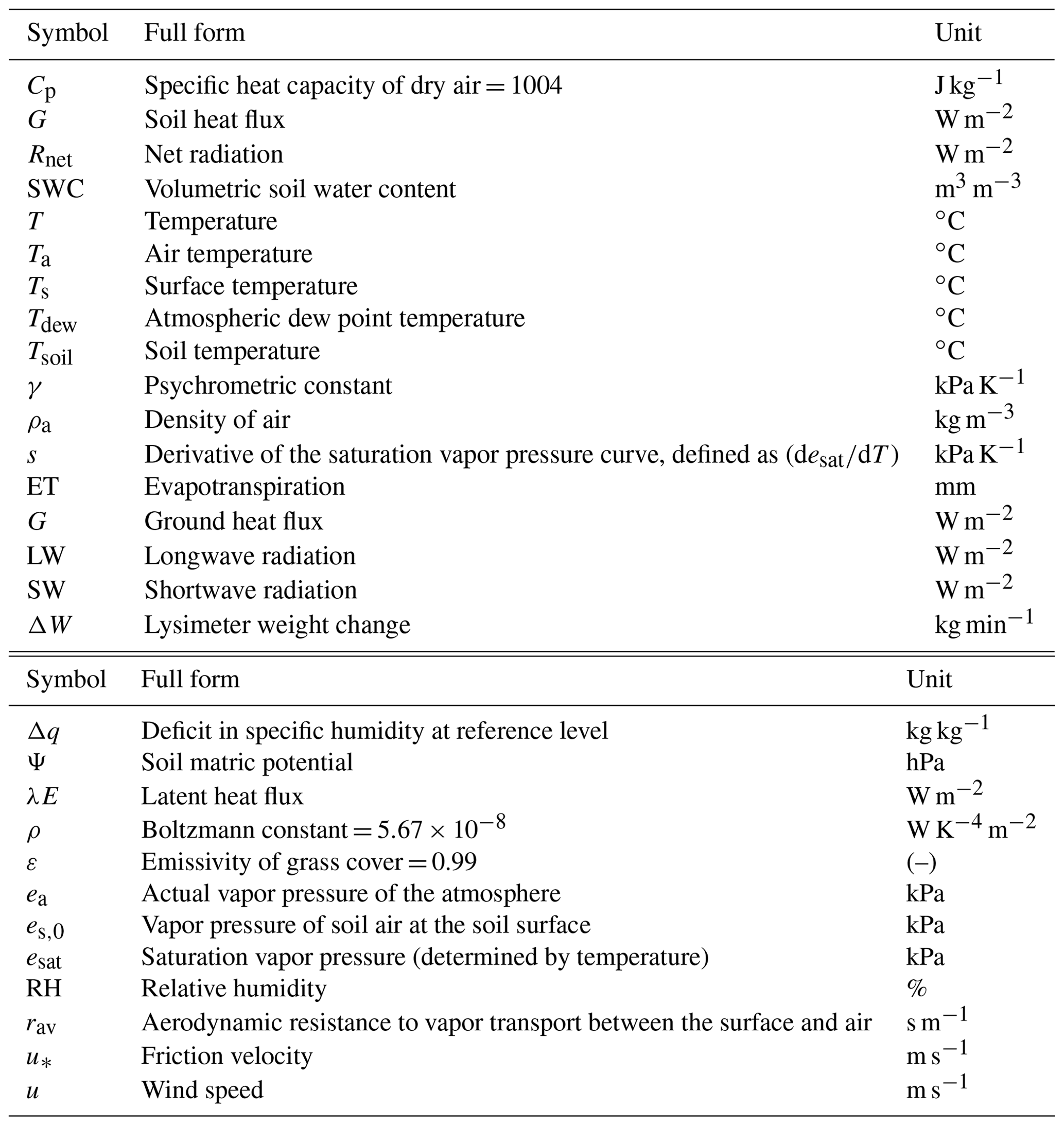
All data investigated in this study originate from the experimental field site Majadas de Tiétar, Cáceres, in Extremadura, Spain (39∘56′25.12′′ N, 05∘46′28.70′′ W). All variables used are summarized in Table B. The average diel Ta is 16.7 ∘C, with a diel minimum and maximum Ta of 3.1 to 12.5 ∘C in January and 18.6 to 39.8 ∘C in August. The rain mainly falls between October and April, with mean annual amounts of ca. 650 mm, with large interannual variations (El-Madany et al., 2020). The mean annual potential evapotranspiration calculated with the Priestley–Taylor equation (Knauer et al., 2018) amounts to 1524 mm yr−1. The ecosystem is a typical Mediterranean semi-arid tree–grass ecosystem (dehesa) with low-density oak tree cover (Quercus ilex (L.) of ∼ 20 trees per hectare) (Bogdanovich et al., 2021).
The herbaceous layer consists of native annual grasses, forbs, and legumes (Migliavacca et al., 2017). The growing season for the herbaceous layer begins after the first rains after summer (typically in mid-October) and is inhibited by low temperatures in winter before peaking in spring before the dry season (Luo et al., 2020). During the dry season, the herbaceous species are inactive until the return of rain (Perez-Priego et al., 2018), and bare soil is visible below the dry biomass. The mean leaf area index of the herbaceous vegetation ranges between 0.25±0.07 m2 m−2 in summer and 1.75±0.25 m2 m−2 at the peak of the growing season in spring (El-Madany et al., 2021), with the same seasonal dynamics in the vegetation height that varies between 0.05 and 0.20 m (Migliavacca et al., 2017). Biocrusts are not present at the site (Perez-Priego et al., 2018). The site is managed with low-intensity grazing by cows during the growing season (El-Madany et al., 2018). An exclusion fence of ∼50 cm height was used to avoid cows stepping into the lysimeters. However, the fence was close enough to allow grazing of the columns in order to keep the vegetation on lysimeters comparable with the rest of the plot (picture shown in Fig. A1). The soil is formed of alluvial deposits and classified as Abruptic Luvisol (IUSS Working Group WRB, 2014), with a sandy topsoil of 74 % sand, 20 % silt, and 6 % clay (Nair et al., 2019). A clay layer rests at a variable depth between 30 and 100 cm. Although the trees also play a role in the water balance at the ecosystem scale, herbaceous vegetation dominates ET (Perez-Priego et al., 2017). This work focuses on the water fluxes in open areas where lysimeters are located (Migliavacca et al., 2017).
2.1.1 Lysimeter technical specifications
The site is equipped with three lysimeter stations, each containing two weighable, high-precision, high-density polyethylene lysimeters (Umwelt-Geräte-Technik GmbH, Müncheberg, Germany), for a total of six columns. Each column has a 1 m2 surface area and 1.20 m column depth and is situated on a weighing system consisting of three precision shear stress cells, respectively (model 3510, Stainless Steel Shear Beam Load Cell; VPG Transducers, Heilbronn, Germany). The weight measurements are collected every 1 min, with a measurement precision of 10 g (0.01 mm). Each lysimeter station is equipped with a lower boundary control system to avoid deviations from natural conditions due to the isolation of the lysimeter columns (Groh et al., 2016). Porous ceramic bars at the bottom of the lysimeters maintain the soil water potential within the column to be comparable with the soil surrounding them. Soil temperature (Tsoil; ∘C) is controlled with a heat exchange system. Buried at the bottom in each lysimeter are 6 m tubing systems that are connected to tubing systems buried at the same depth in the surrounding soil. Pumping of water through the system in a closed loop regulates the soil temperature within each lysimeter column by heat exchange (Podlasly and Schwärzel, 2013).
Soil water content (SWC) and Tsoil are measured every 15 min within the columns at 0.1, 0.3, 0.75, and 1 m depth (UMP-1, Umwelt-Geráte-Technik GmbH, Müncheberg, Germany). Soil matric potential (Ψ; hPa) is measured every 15 min at 0.1 m depth with a porous ceramic cone full-range potential force (pF) meter (ecoTech Umwelt‐Meßsysteme GmbH, Bonn, Germany).
The lysimeters were installed in 2015 by excavating undisturbed soil monoliths from open grassland areas. General aspects of the excavation method are described in Reth et al. (2021). The natural herbaceous vegetation cover was preserved. Pictures of the lysimeter columns and an aerial photograph of the site and experimental setup are shown in Fig. A1. The stations have a 104, 91, and 24 m distance to each other, respectively. The closest tree is ∼9 m away. We analyze a period of 1 year from 1 June 2019 to 31 May 2020.
2.1.2 Ancillary measurements outside the lysimeters
For partitioning the lysimeter weight changes (ΔW; kg min−1) into different water fluxes and modeling (see Sect. 2.2.1, 2.3.2, and 2.3.3), we used additional field measurements collected every 30 min. Meteorological variables monitored are rain, which is measured with a weighing rain gauge (TRwS 514 precipitation sensor, MPS systém Ltd., Slovakia), Ta, and RH at 1 m (Pt-100 and capacitive humidity sensor CPK1-5, MELA Sensortechnik, Germany). Tdew was calculated based on Ta and RH (see Appendix C). Actual vapor pressure (ea; hPa) is calculated from Ta and RH.
Short- (SW; W m−2) and longwave (LW; W m−2) downwelling (↓) and upwelling (↑) radiation of the herbaceous layer was observed with a net radiometer (CNR4, Kipp & Zonen, Delft, the Netherlands) at a measurement height of ∼2 m. Ts is calculated from LW measurements (equations in Appendix C). Ground heat flux (G; W m−2) was monitored with soil heat flux plates (Heatflux Ramco HP3, McVan Instruments Pty Ltd, Mulgrave, Australia).
Tsoil and SWC were measured along a profile outside the lysimeters at 0.05, 0.10, and 0.2 m depth, respectively (ML3 ThetaProbe Soil Moisture Sensor, Delta-T Devices Ltd, Burwell, Cambridge, UK).
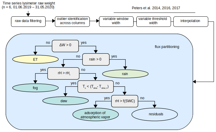
Figure 1Overview of the lysimeter data processing to determine non-rainfall water (NRW) inputs. White rectangles represent the steps of the preprocessing chain before flux partitioning. The preprocessed time series is then classified into the different vertical water fluxes based on a decision tree structure shown in the light blue box. Gray rectangles stand for the decision nodes and ellipses for the endpoint nodes. The decision tree is adapted from Zhang et al. (2019a). Detailed information on the choice of parameters, RHt, Tdewc, and f(SWC), and their uncertainty are given in Sects. 2.2.1 and 4.
Fluxes of latent heat (λE; W m−2), wind speed (u; m s−1), and friction velocity (u*; m s−1) were measured by an eddy covariance (EC) system, consisting of a sonic anemometer (R3-50, Gill Instruments Limited, Lymingon UK) and an infrared gas analyzer (LI-7200, LI-COR Biosciences GmbH, Bad Homburg, Germany) at 1.6 m sampling height and targeting the herbaceous layer (Perez-Priego et al., 2017). For further details on the EC data processing, see El-Madany et al. (2018).
2.2 Data analysis
2.2.1 Lysimeter data processing
The processing of lysimeter data comprises several steps, including (a) raw weight data filtering, (b) time series smoothing, and (c) flux partitioning, which are elaborated on below. The processing workflow is displayed in Fig. 1. All codes used in the analysis are available for reproducibility in the open-source R environment for statistical programming (R Core Team, 2020). See the data and code availability statement for more details.
2.2.2 (a) Raw data processing
Changes in the water reservoir through the lower boundary system and lysimeter column weights are added. Outliers are filtered out by setting plausible threshold values, i.e., −0.5 kg min kg min−1 (Schrader et al., 2013). Additionally, outliers within these threshold values were identified by comparing ΔW across the six columns. If ΔW is due to rain, then we expect similar responses across lysimeters. In contrast, if only one lysimeter column shows an anomalous ΔW, then we considered this to be an artifact (e.g., small animals such as snakes or rabbits coming into contact with the column or issues with the boundary control) that can be removed from the time series (Hannes et al., 2015). To identify these values, we calculated the mean ΔW of all six lysimeters for an interval i of 1 min. This value was then subtracted from the individual ΔW measurements during i. The resulting value is a normalized weight change (ΔWnormalized,i; kg) for each column. Then, an average standard deviation (; kg) was calculated from to . are replaced by not available (NA).
(b) Time series smoothing
Time series smoothing is necessary to remove noise from the time series before the partitioning and data analysis based on ΔW (Schrader et al., 2013). Since noise in this type of data is not constant in time due to wind, for example (Nolz et al., 2013), we apply a routine with adaptive averaging window widths (ω) and adaptive ΔW thresholds (δ) (AWAT) from Peters et al. (2014, 2016, 2017). As an intermediate result, the AWAT algorithm produces a step function of the lysimeter weight. Last, a smoothing of the 1 min resolution time series is performed using a spline interpolation. We chose this routine because the authors included a processing step developed specifically for dew conditions (Peters et al., 2017). In our application, the parameter ω varied between 3 and 31 min and δ between 0.01 and 0.05 mm. A detailed overview of the algorithm and an evaluation of the performance have been compiled in Peters et al. (2017) and Hannes et al. (2015). If one out of all of the columns was measuring more than 16 h of weight gain during 1 d, then the full day was excluded for the analysis for the respective column. Due to technical problems that became obvious after data processing, lysimeter column number 4 was completely excluded from further analysis. After the smoothing, the time series are aggregated to a 5 min resolution to further decrease the remaining influence of noise for the subsequent step of flux partitioning, particularly for values close to zero.
2.2.3 (c) Flux partitioning
The filtered time series of ΔW is divided into six different water fluxes, assuming that, in 5 min intervals, only one process prevails over the others. Negative ΔW is always classified as ET. Positive ΔW is separated into different flux categories in a decision tree structure considering additional meteorological data, as illustrated in Fig. 1. At the second decision node, we check if the rain gauge identifies a rain event during the period of weight increase. If true, then all positive ΔW are classified as rain during the 30 min before and after the event. This period was selected to match the measurement interval of rain gauges which is 30 min. If false, e.g., in the absence of rain, then the RH is evaluated.
Theoretically, fog occurs at a RH of 100 %. We noticed, however, that the maximum saturation values varied, depending on the sensor, with values between 98 % and 104 % (Fig. G1). We therefore decided to set a RH threshold (RHt) that is based on the data distribution of the sensor to account for the individual uncertainty when the air is nearly saturated, for systematic biases and for drifts. In our study, ΔW is attributed to fog when RHt=97.1 %, which is the 90th percentile of the RH sensor records measured at 1 m height.
If neither fog nor rain is detected, then we compare Ts with Tdew. Between the top of the canopy and the soil surface, however, there is a large temperature gradient which is also reflected in dew amounts (Kidron, 2010). Since the installation height of the sensor is 1 m, we needed to approximate a value that better reflects Tdew at the height of the condensation surfaces. Despite a reference height of 0.1 m generally being used (Monteith, 1957), we approximated 10 cm, which reflects the average canopy height of the herbaceous layer. To include the effect of the height difference, we compared sensors installed at 0.1 and at 1 m height during a measurement campaign of 2 months in spring 2021. The results show that the median temperature difference between the 0.1 and 1 m sensor height is 1.4 ∘C with an interquartile range (IQR) of 1.2 ∘C. Dew was therefore assigned when ), where Tdew,c is set to 1.4 ∘C. Note that the measurement height and the offset value should be site-specifically adapted, depending on the height of the condensation surfaces.
If no dew was detected, then ΔW could be potentially attributed to the soil adsorption of atmospheric vapor (Zhang et al., 2019a). Adsorption occurs, however, at specific soil hydraulic and meteorological conditions given by a relation between Ψ and atmospheric RH. Those have been observed in the laboratory (Camuffo, 1984; Arthur et al., 2016) and suggested from field observations (Kosmas et al., 2001; Uclés et al., 2015; Zhang et al., 2019b). For adsorption, Ψ falls below (or is less negative than) a given threshold. This threshold can also be expressed in terms of SWC, given the relationship between Ψ and SWC through the soil water retention curve. In order to integrate this knowledge into the classification of adsorption, measurements of RH and SWC were analyzed for the periods where adsorption conditions were identified based on modeling (see Sect. 2.3.3). For these periods, we fit a nonlinear quantile regression (90th percentile) to measurements of RH and SWC. This nonlinear relationship is depicted in Fig. H1 in the Appendix. Although, for the description of this relationship, multiple empirical functions exist for samples measured in the laboratory under equilibrated conditions, they do not apply to our case due to the different observation ranges of RH and SWC at our site (see Fig. H1 for examples). When RH≥f(swc), then the soil adsorption of atmospheric vapor is assigned to positive ΔW. When RH<f(SWC), then we classify the flux as residual. Example lysimeter weight evolution and the assigned flux categories for a week with and without rain are shown in Fig. D1 in the Appendix.
Fluxes are presented in the Sect. 3 as the mean and standard deviation across the five lysimeter columns.
The results of the partitioning algorithm, in addition to the uncertainty in the NRW inputs, might be sensitive to the set of parameters and threshold values used at each node. Therefore, the impact of the choice of threshold parameters on the flux uncertainty was tested. To do so, we defined a parameter set that describes the upper and lower limit of the parameter values, specifically RH % and Tdew,c=[0, 1.5] ∘C. The parameter values tested cover the ranges of the threshold values for RH and Ts, which are currently used in similar studies to identify fog and dew conditions (e.g., Feigenwinter et al., 2020; Zhang et al., 2019b). We then ran forward the partitioning algorithm with all the combinations of the parameters. The uncertainty in the calculated fluxes was then characterized based on the IQR of the resulting flux quantities, as will be shown in Sect. 3.1.
2.3 Quantitative validation and benchmarking of the NRW assignment
We test the plausibility of inferred water fluxes by comparison against direct measurements (for rain and ET), in the absence of respective direct measurements derived with alternative measured variables for NRW by benchmarking (for fog), and by comparison against model predictions (for dew and adsorption).
2.3.1 Identification of fog conditions and their separation from dew
Since clear-sky conditions and the amount of humidity present in the air is a key factor for both dew and radiation fog formation, their distinction is challenging. Measurements from visibility sensors are therefore used in addition to RHt to classify fog unambiguously (e.g., Feigenwinter et al., 2020; Riedl et al., 2022). Given that at the experimental site visibility sensors are not available, we use LW radiation to benchmark fog occurrence in our analysis.
When a fog layer contains a sufficient amount of liquid water, then the suspended droplets cause an optically thick layer obstructing LW radiation from and to the sky (Wærsted et al., 2017). Under such conditions, measurements of LW↓ and LW↑ within the fog layer should be identical. Therefore, we compare the ratio of LW↓ and LW↑ in periods classified as fog to the periods classified as dew from the ΔW partitioning. We used the nonparametric Mann–Whitney U test to evaluate statistically significant differences between the radiation patterns associated with both conditions. This was applied to a period of 3 years, from 1 January 2018 to 31 December 2020, to increase the number of events for better statistical robustness.
2.3.2 Modeling dew
Dew is modeled as a negative latent heat flux calculated based on models originally developed for determining evapotranspiration, i.e., (i) the Penman–Monteith (PM) equation (Monteith, 1965), which combines processes related to radiative energy and vapor pressure deficit (previously applied for dew in various forms by e.g., Jacobs et al., 2006; Aguirre-Gutiérrez et al., 2019; Groh et al., 2018), and (ii) equilibrium evaporation (previously applied for dew by Uclés et al., 2014).
We implemented the models as described in Ritter et al. (2019) and Jacobs et al. (2006) (Eq. 1) and in Uclés et al. (2014) (Eq. 2).
where λE (W m−2) is the latent heat flux, s (Pa K−1) is the derivative of the saturation vapor pressure curve defined as (), γ (kPa K−1) is the psychrometric constant, Rnet is net radiation (W m−2), G is the soil heat flux (W m−2), ρa (kg m−3) is the density of air, and Δq is the deficit of specific humidity at the reference level (kg kg−1). rav is the aerodynamic resistance to vapor transport between the surface and the air (s m−1) and was derived with an empirical relationship based on u* (Thom, 1972).
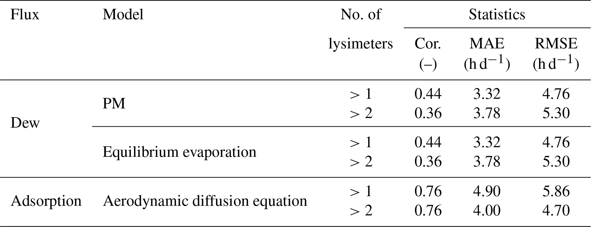
For both equations, dew occurs when λE<0 and ∘C) (as explained in Sect. 2.2.1). This approach has been reported to be suitable for detecting potential dew conditions and for analyzing dew frequency and duration. But it is limited in reproducing dew yields (Ritter et al., 2019). Hence, we focus on comparing condition lengths rather than yields, since we aim to validate dew detection by the partitioning routine. Measured flux durations were compared to the respective model estimates modeled flux using correlation (Cor.), mean absolute error (MAE), and root mean squared error (RMSE; full equations in Appendix C).
2.3.3 Modeling adsorption
Adsorption conditions were identified based on the vertical humidity gradient near the surface. We implemented the rearranged aerodynamic diffusion equation originally used by Milly (1984) and previously applied for modeling adsorption by Verhoef et al. (2006) as follows:
The target value es,0 (kPa) is the vapor pressure of soil air at the surface. ea (kPa) is the vapor pressure of the atmosphere, and Cp (J kg−1 K−1) is the specific heat capacity of dry air at constant pressure. The other parameters are the same as in Eq. (1). When , the gradient-driven vapor flow is towards the soil surface. Note that λE is the target variable in the dew models (Eqs. 1 and 2) but a predictor variable in the adsorption model (Eq. (3). For λE in Eq. (3), we used high-quality filtered measurements from EC. Again, we only compared the simulated daily duration of suitable conditions of atmospheric adsorption against the results obtained with the lysimeter weights partitioning, and we constrained the comparison to periods when .
3.1 Diel and seasonal changes in water fluxes
Figure 2 shows the fingerprint of the lysimeter ΔW induced by ET, rain, and NRW, assigned water flux types (exemplarily shown for lysimeter column 6), and RH, respectively, together with mean diel SWC at 0.05 m depth and the maximum diel Ts range.
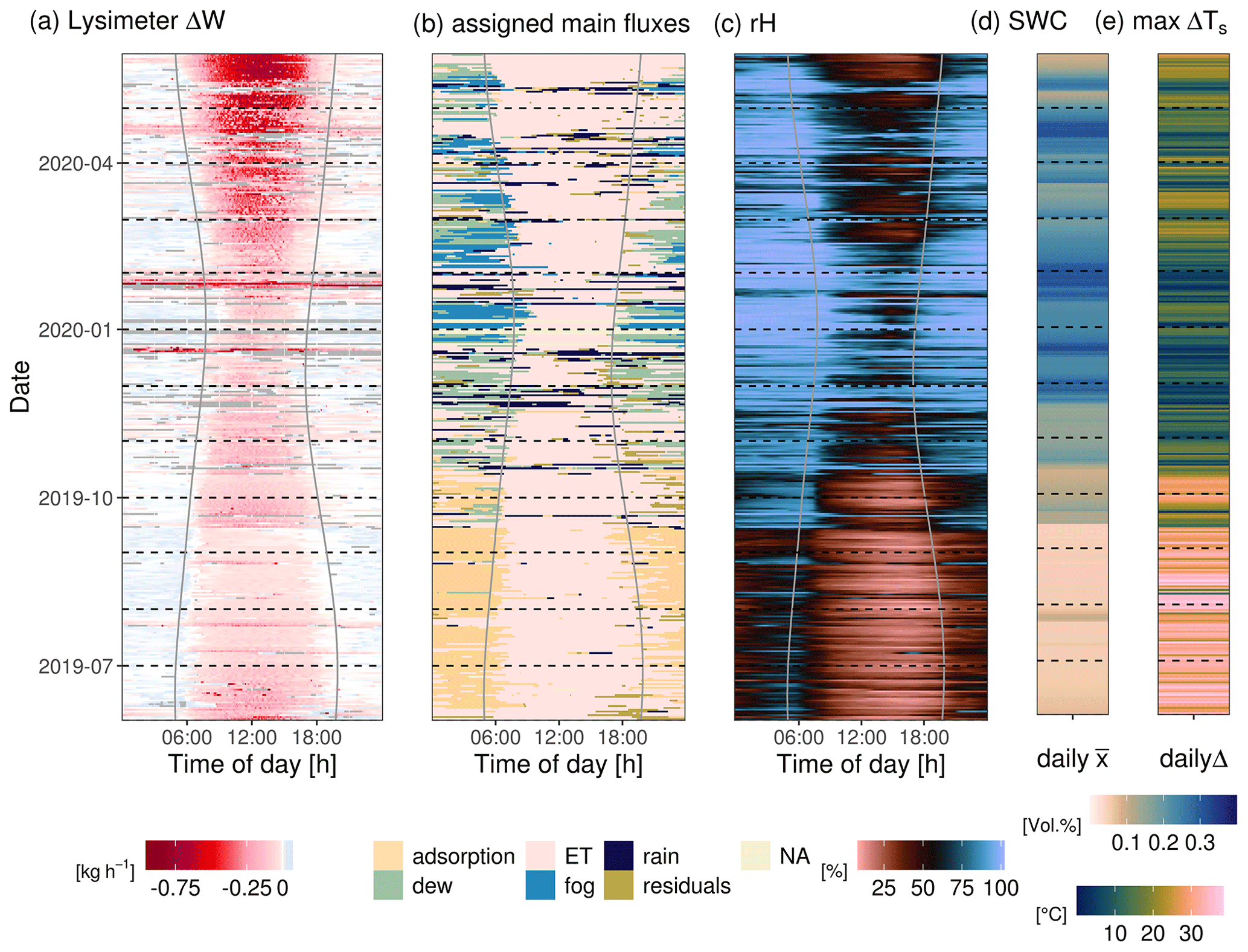
Figure 2Diel and seasonal dynamics of (a) lysimeter weight changes, (b) assigned flux types, both from lysimeter 6, and (c) RH measured at 1 m height. Solid vertical lines mark sunrise and sunset, respectively, determined with the geographic coordinates of the field site. Mean SWC at 0.05 m depth and maximum diel difference in Ts are displayed as diel measurements in panels (d) and (e).
Lysimeter ΔW are mainly negative between sunrise and sunset (Fig. 2a), i.e., water is lost from the column due to ET. After sunset, however, they are zero or positive during most of the year, indicating water input. This diel pattern is consistent across seasons, following the seasonal daylight variability. The flux classification reveals seasonal differences in the prevailing NRW fluxes (Fig. 2b). At the beginning of June, atmospheric adsorption mainly occurs during the early morning, before sunrise. From July to September, the length of the adsorption period increases, and the onset shifts towards earlier in the night. In this period, the diel variability in RH is relatively low (Fig. 2c), SWC at 5 cm depth is below 10 %, and Ts oscillates up to an amplitude of 35 ∘C d−1 (Fig. 2d and e). A rain event in late July increases SWC and is followed by some days of increased ET, which also prevails during nighttime.
A rain event in late September leads to longer-lasting increases in SWC and RH. Such conditions are typically associated with vegetation re-greening. ET and dew alternate during night-time. Frequent rain events in November and December are accompanied by dew and fog becoming the dominant NRW inputs until the end of the measurement period in April.
On most days, the average NRW inputs is <0.2 mm d−1 (Fig. E1). Yields of <0.2 mm d−1 are observed on 54 d distributed throughout the year. During the dry season, NRW inputs are predominantly between 0.1 and 0.2 mm d−1, while over the wet season, the yields are typically small at <0.2 mm d−1. The maximum recorded daily NRW inputs was 2.42 mm d−1 on 13 May 2020 between several small, consecutive rain events.
NRW fluxes occur for at least 3 h during 297 d (81 % of the year), with a mean duration of 6 h per day of occurrence.
The weekly sums in Fig. 3 illustrate that the seasonal dynamics are consistent across lysimeters. The ecosystem receives atmospheric water at any time of the year but with shifting relative relevance of the water flux types during the wet and the dry season. Rain is the dominant liquid water input (i.e., it contributes more than 50 % of the weekly water input) during 29 weeks, since its total amount is usually much greater than NRW inputs, whereas NRW inputs are dominant in 24 weeks. They are even the only water input during 15 weeks, with adsorption as exclusive water input in 10 weeks of the year during the dry season.
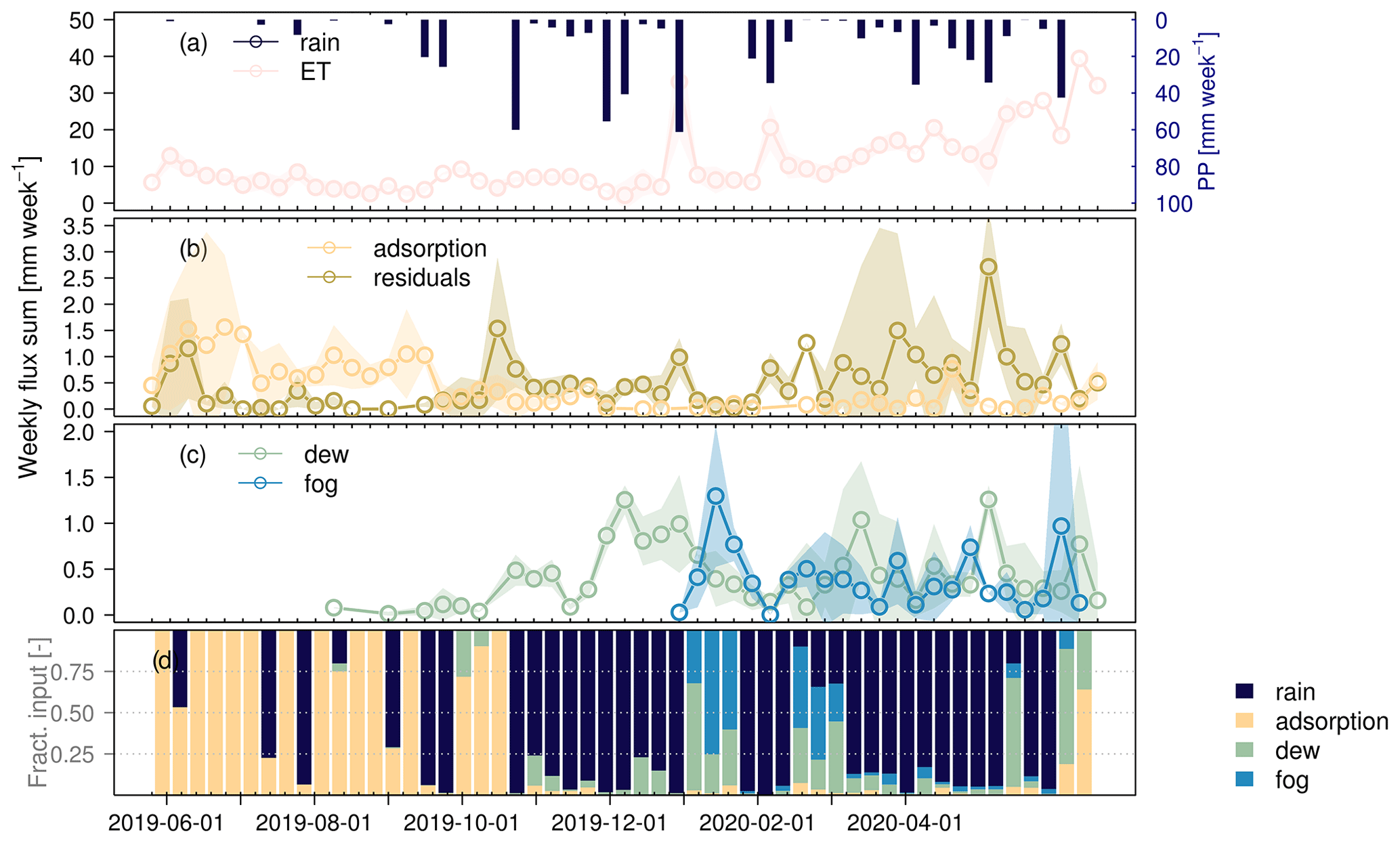
Figure 3Median of weekly flux sums across lysimeters for (a) ET and rain, (b) adsorption and noise, and (c) dew and fog. (d) Relative contributions of rain and NRW inputs to total water input per week, respectively. Shading indicates the variability across lysimeter columns expressed as an interquartile range (IQR).
During the dry season, the median contribution of adsorption is 0.9 mm per week, whereas dew and fog contribute <0.5 mm per week. With ET amounting on average to 5.7 mm per week, adsorption compensates on average for 19 % of the weekly water loss through ET during summer, ranging between 8.0 % at the beginning of June to 42.5 % at the beginning of September. During the wet season, the median contribution of dew and fog is 0.43 and 0.38 mm per week, respectively. Dew and fog occurrence is synchronized with rain with regard to the seasonal occurrence (in the wet season), and therefore their relative contribution to the water input on a weekly scale is small (see Fig. 3d).
3.2 Water fluxes and their consistency with measurements and theory
The cumulative measured rain is 565.0±11 mm as an average across the five lysimeters. Thereby, the difference between the maximum and minimum across the lysimeters is 30.7 mm, which is an absolute deviation of 5 % between columns. For comparison, the rain gauge recorded 597 mm of rain during the same time period. The underestimation of the estimates from lysimeters compared to the rain gauge, in addition to the deviation between columns, is mainly caused by a few large rain events in January 2020 (Fig. 4a). The cumulative measured ET across lysimeters is 570.7±20 mm. The annual cumulated difference between lysimeters is 46.7 mm. Annual cumulative ET determined through EC measurements is 619.0 mm. As in the case of rain, the ET estimates deviate strongest in winter, which indicates a technical problem during days with rain at this time of the year, while estimates are more consistent during the rest of the study period (Fig. 4d).

Figure 4Comparison between cumulative (a, c) and mean diel (b, d) observations of rain and ET between the lysimeter and rain gauge (a, b) and lysimeter and EC (c, d). The points and vertical error bars indicate mean and standard deviation between lysimeter columns, which include measurement uncertainty and spatial variability.
Descriptive statistics of the annual sums of NRW inputs across lysimeter columns are summarized in Table 1. The average annual NRW sum amounted to 41.9 mm, with individual contributions of 6.6 mm from fog, 14.1 mm from dew, and 21.2 mm from adsorption. The differences in flux sums across lysimeters for all NRW inputs are relatively larger than for rain and ET, with coefficients of variation around 40 %. The largest relative annual deviation between columns was found for adsorption, with a difference of 20.0 mm. But the flux which is most affected by the threshold parameter in the lysimeter flux partitioning is fog, which can be seen in Table 2. The IQR for the fluxes decreases the later in the partitioning scheme in which the respective flux is estimated (Fig. 1). Thereby, for dew and adsorption, the spatial variability between lysimeter columns (IQR in Table 1) exceeds the range of uncertainty related to the partitioning parameters (IQR in Table 2). The largest relative contribution to the mean total NRW input is adsorption (50 %), followed by dew (34 %) and fog (16 %).
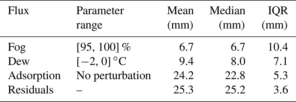
Table 1Mean, median, and interquartile range (IQR) and minimum and maximum annual sum of individual NRW fluxes across lysimeter columns. All values are reported in millimeters per year (mm yr−1).
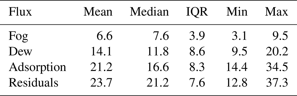
Table 2Uncertainty related to the flux partitioning parameters. The table summarizes the annual mean and median fluxes of all lysimeters across all combinations of parameters in the given ranges. Additionally, their interquartile range (IQR) is provided.
Plausibility of the partitioning parameter RHt for the distinction between fog and dew was tested in two steps. First, conditions of thick fog were visually assessed from the digital camera imagery (exemplar shown in Fig. G1). During these conditions, a median ratio of LW↓ over LW↑ of 0.98 was found (Fig. G2). During non-foggy conditions, the median ratio is lower (0.88). The difference is statistically significant (p<0.001). This shows that, during fog, LW↑ and LW↓ are close to equilibrium. The positive lysimeter ΔW assigned to fog based on RHt=97 % is also closer to the radiation equilibrium (median = 0.9) compared to dew (median = 0.84; Fig. 5). The difference between the two categories is statistically significant (p<0.001), despite the distributions overlapping. This applies also to RHt of 100 % or 95 %, but the median radiation ratios during lysimeter-classified fog conditions shift to 0.94 and 0.86, respectively (see Fig. G3).
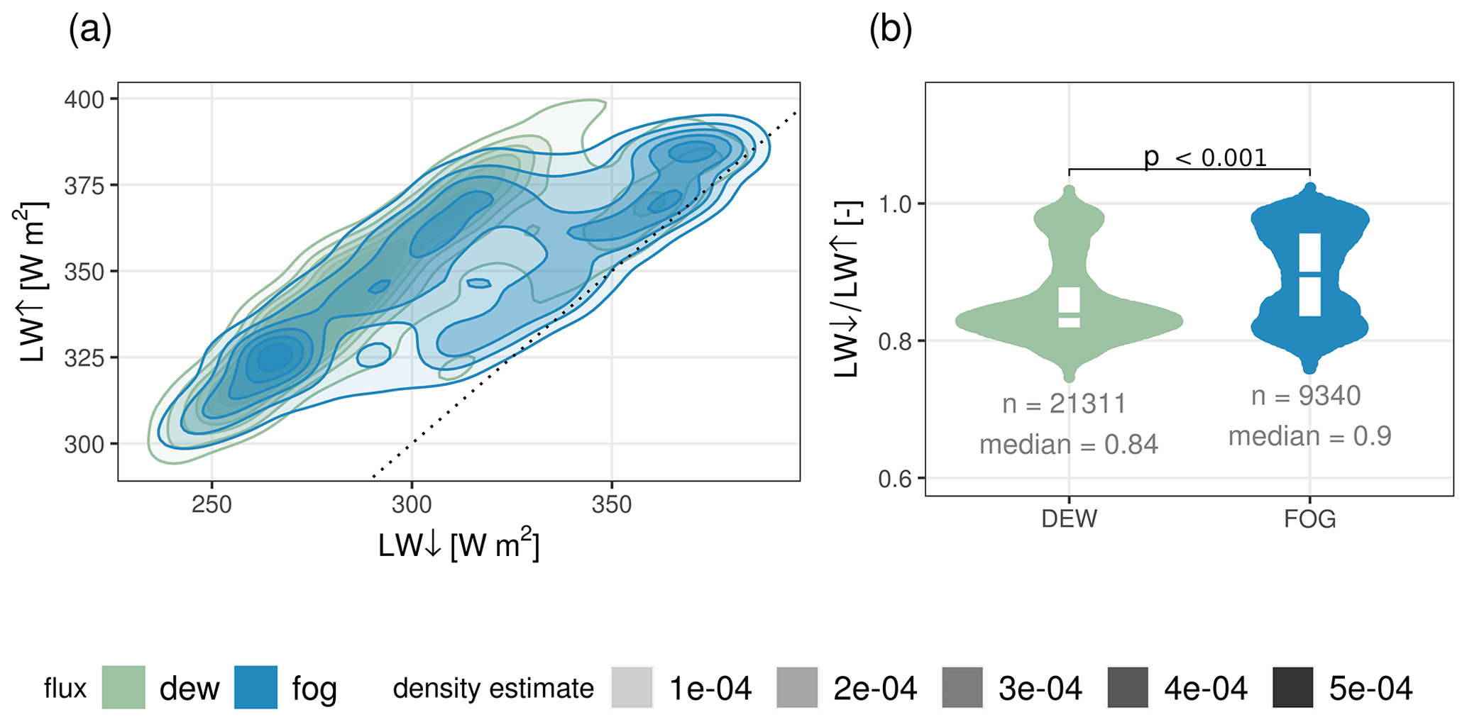
Figure 5Comparison of upward (↑) and downward (↓) longwave (LW) radiation during the conditions classified as fog and dew from the flux partitioning of lysimeter weight changes. Panel (a) illustrates the smoothed kernel density estimate, with the black dotted line displaying the identity line. Panel (b) illustrates the distribution of radiation ratios during dew and fog conditions. The difference between the distributions is statistically significant, with a significance level of p<0.001.
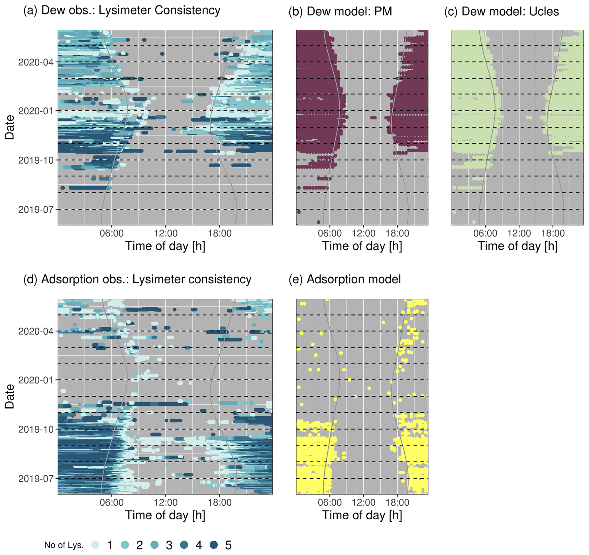
Figure 6Diel and seasonal dynamics of the consistency of inferred (a) dew and (d) adsorption across all lysimeters. The modeled occurrence is presented for dew from (b) the Penman–Monteith model (PM) and (c) equilibrium evaporation model and for adsorption using (e) the aerodynamic diffusion equation. Solid lines mark sunrise and sunset, as determined by the geographic coordinates of the site.
To assess whether the thermodynamic requirements for dew and adsorption are met at our site, we compare the lysimeter-inferred observations of dew and adsorption with their potential occurrence determined with the models from PM, equilibrium evaporation, and the aerodynamic diffusion equation (Fig. 6). Our results show that the measured fluxes are temporally consistent with model results regarding both diurnal and seasonal dynamics.
In general, the Majadas site has suitable conditions for dew between October 2019 and end of May 2020, from sunset to sunrise. The statistical metrics for the comparison of daily dew duration between lysimeters and models are summarized in Table F1. They show that, overall, the models suggest a longer duration of dew conditions by 3 and 5 h d−1. Model statistics from PM and the evaporation model are not deviating from each other, indicating that, in our application, no difference between the simplified and full PM model is detectable. In the case of adsorption, the lysimeter-based estimates agree better with the model predictions (Table F1). When comparing only measurements where at least two out of the five lysimeters show weight increases assigned to adsorption, MAE and RMSE decrease from 4.9 to 4.0 h d−1 and from 5.9 to 4.7 h d−1, respectively. In addition, the agreement of lysimeters is overall stronger during adsorption than during dew conditions (Fig. 6). Single lysimeters, however, frequently also measured adsorption until midday and before sunset.
In this study, we showed that the climatic conditions in a semi-arid Mediterranean savanna site fulfill the thermodynamic requirements to induce the diel cycles of evaporation and condensation at almost all times of the year. This finding is based on a large weighing lysimeter and a few ancillary measurements. The routine applied to detect and distinguish NRW inputs is benchmarked, with measurements of LW and validated against models based on energy balance and moisture gradients, with regard to the occurrence of the process.
4.1 Non-rainfall water frequency, duration, and amounts
We found that NRW occurs frequently at our site, in line with previous research in such a climate regime. The occurrence of both adsorption and dew was shown by Zhang et al. (2019b). We support their observation that dew formation and adsorption dominate at different times of the year. Regular dew formation (120 to 200 nights per year) has been reported across sites (Tomaszkiewicz et al., 2015). In a similar semi-arid steppe ecosystem in Spain, the mean number of days per year with suitable conditions for dew formation was 285 d (Uclés et al., 2014). However, this finding is based on measurements with micro-lysimeters consisting of PVC sampling cups with <0.1 m length, for which it has been shown that they tend to overestimate dew when compared with alternative sampling approaches (Kidron and Lázaro, 2020; Kidron and Kronenfeld, 2020a, b). Our observation that especially nights are prone to the formation of NRW is also documented in the literature. Dew formation length has often been reported to correlate with the length of the night (Tomaszkiewicz et al., 2015) and was, in another Spanish site, reported to last on average 9.3±3.2 h per night (Uclés et al., 2014). In contrast, for adsorption, reported observation times differ. Kosmas et al. (1998) observed the flux to occur mainly between 00:00 and 06:00 LT, and Saaltink et al. (2020) also found suitable nighttime conditions for adsorption through a reversed gradient of vapor concentration between soil and atmosphere from lysimeter observations and confirmed it with a fully coupled numerical model. Yet, Verhoef et al. (2006) found adsorption occurring during the afternoon and ceasing at night. Since changes in Ts and their effects on the phase equilibrium of water are one of the main controlling factors of adsorption, the different findings between studies could be related to site-specific timing of surface exposure to radiation.
Next to the diagnosed occurrences, the NRW input amounts we determined are also within the range of previously reported estimates for similar climate regimes. At our study site of Majadas, the largest annual NRW contribution is adsorption (21.2 mm yr−1). This value is relatively low, compared to sites close to the sea, where values of 81 mm yr−1 (Saaltink et al., 2020) and 26 and 110 mm between April and October have been reported (Kosmas et al., 2001). But it matches well with observations from Qubaja et al. (2020), who measured the annual adsorption of 14 mm yr−1 using flux chambers in a semi-arid pine forest in Israel. Daily adsorption was reported to compensate for 25 % and 50 % of ET in a Spanish olive orchard (Verhoef et al., 2006) and even 93 % of ET in the Negev (Florentin and Agam, 2017). With a maximum compensation of 42 % per week, our findings are comparable to the observations in the olive orchard. However, it should be noted that the two cited studies covered time periods of only several days, and therefore, the variability in these percentages across the season is not known.
Furthermore, dew and fog quantified here at 14.4 and 6.6 mm yr−1, respectively, are within the range reported from other sites which are, depending on the site, 4 and 39 mm yr−1 for dew (Tomaszkiewicz et al., 2015) and 1.3 and 50 mm yr−1 for fog (Zhang et al., 2019b; Kidron and Starinsky, 2019). It is important to remark, however, that part of the large variability concerning the length of the occurrence and condensation rates for NRW inputs could be related to biases of the measurement devices. Many former studies based on micro-lysimeters likely overestimated NRW inputs due to greater heat loss through the walls compared to the surrounding unperturbed soil (Kidron and Kronenfeld, 2020b). Despite the current version of large weighing lysimeters being designed with lower boundary control in order to prevent temperature deviations from the surrounding soil, the extent to which heat loss through their walls will affect NRW has yet to be evaluated at sites with suitable instrumentation, particularly since NRW is sensitive to deviations in Ts (Yokoyama et al., 2021). Such a comparison was not possible in our instrumental setup because Ts was derived from measurements in one location only, which was situated outside the lysimeters (Fig. A1).
4.2 Impact of methodological uncertainty
We found differences in the absolute annual NRW sums between individual lysimeters that can be attributed either to (i) spatial variability (heterogeneity) in the soil and vegetation characteristics affecting the energy balance or (ii) instrumental and methodological uncertainty. Particularly for the latter, external disturbances by wind or animals and internal disturbances such as data gaps and data processing have been shown to alter results significantly (Schrader et al., 2013; Nolz et al., 2013). Developing processing routines for raw data from large weighing lysimeters has challenged researchers during the last decade (Schrader et al., 2013; Peters et al., 2014, 2016, 2017; Hannes et al., 2015). To assess the robustness of the processing, we compared rain across lysimeters, as rain is expected to be similar across nearby lysimeters and heterogeneous soils and vegetation. The variation in rain across lysimeters is only 5 %, which is of a similar magnitude to that reported in other studies (Hannes et al., 2015; Schneider et al., 2021). However, NRW sums often deviated between different measurement instruments and manual sampling (Kidron and Starinsky, 2019; Kidron et al., 2000). Unfortunately, the quantitative validation of NRW sums was not possible in our current study. Model simulations independently confirmed that the conditions at night are suitable for NRW, although, especially for dew, the simulations showed that the potential for dew formation is generally longer than actual occurrence measured with lysimeters.
Particularly at our field site, the spatial heterogeneity of soil and vegetation characteristics can affect our results (Nair et al., 2019). In fact, dew and adsorption amounts are both reported to vary substantially with the surface cover type (Uclés et al., 2016), soil exposure (Kosmas et al., 2001), shading hours (Uclés et al., 2015), distance from trees (Verhoef et al., 2006; Qubaja et al., 2020), and soil texture, particularly clay and sand content (Kosmas et al., 2001; Orchiston, 1953; Yamanaka and Yonetani, 1999).
Vegetation height and density affect the radiative exchange of the soil surface and the plant canopy, affecting dew formation occurrence and amount (Monteith and Unsworth, 2013). Xiao et al. (2009), for example, observed a positive relationship between maize plant height and the amount of dew formed per night over 2 years. The grass height and leaf area index (LAI) in Majadas change over the season, reaching a maximum in height and density usually in winter and spring (Migliavacca et al., 2017). This is in line with our findings of the occurrence of dew and fog nearly exclusively during the wet season (although it is not possible to separate the effects from meteorological conditions). Unfortunately, no data on plant height and density were collected continuously in the lysimeters columns, which would have allowed the studying of their effect on the amount of dew formation (and fog deposition). However, due to the active vegetation on the lysimeters, the effect of their variation in height and density is represented in our results.
Verhoef et al. (2006) showed in a measurement campaign with eight lysimeters concentrically arranged around a single oak tree that, at the most exposed spots, adsorption was doubled compared to the shaded spot. At our site, there are also individual, sparse trees (Bogdanovich et al., 2021) which cause small-scale differences in shading. Since some lysimeter columns are more exposed than others, part of the deviation in NRW input could be explained by spatial heterogeneity. This is supported by measurements of soil Ψ within the individual columns, which showed that one column had an overall greater mean Tsoil in summer, and the threshold of potential adsorption conditions was reached nearly a full month earlier than in other columns. Micrometeorological variables were, however, not measured individually at each column, and therefore, we have no insight into the exact causes of spatial heterogeneity in dew formation. The applied models both only suggest times of dew formation potential based on measurements at the central facility, while the quantity is derived from weight changes. For the same reason, spatial differences are robust, and follow-up investigations can be targeted towards understanding their causes.
4.3 Distinguishing non-rainfall water formation
Another focus of this study was partitioning the lysimeter ΔW into water flux classes. This approach includes the simplified assumption that one flux is always dominating over the others at each time step. In reality, the fluxes can occur simultaneously, with their relative importance shifting gradually over time (Y. Li et al., 2021). Ideally, we could account for a statistical probability ratio between different NRW inputs per time interval. But current research that is quantifying such ratios is too scarce for generalization (Y. Li et al., 2021). Some studies, therefore, do not distinguish between fog and dew (Groh et al., 2018) or add a category of combined dew and fog (Riedl et al., 2022). Disentangling individual NRW fluxes is nevertheless important because of different respective (i) controlling factors and (ii) implications for the ecosystem. Better knowledge on controlling factors can help to identify potential NRW occurrence, also in ecosystems without specialized measurement devices. The approach applied most frequently in the literature and in this study is based on a discontinuous decision-tree-based classification system which was implemented similarly to that suggested by Zhang et al. (2019a). We deviated slightly from their approach. The chosen temperature offset added to Tdew was used in this study to account for the mean vegetation height. The soil surface, however, will exhibit warmer temperatures during the day. The height of the condensation surface should therefore always be considered.
We further added one node to account for prior knowledge on the controls of adsorption. The prior knowledge for soil adsorption stems, however, from smaller samples at equilibrium conditions in the laboratory (Arthur et al., 2016). Our application to the point measurements of RH and SWC from above and below the soil surface assumes that, by choosing the statistical upper envelope, we can distinguish equilibrium conditions from the remaining noise in the time series as best as possible. Although uncertainty remains about the actual shape of this relationship, this approach gives a more conservative estimate of the adsorption amount and helps prevent overestimation. The validity of this relationship is further confirmed by having a similar shape independently, whether it was derived from the periods when lysimeter measurements unanimously were classified as adsorption (before including residuals as a final node) or deduced from negative EC-derived λE.
The advantage of the discontinuous decision-tree-based classification is that it is applicable widely because the necessary data are commonly measured. The disadvantage is that the selection of the parameters and thresholds in the classification algorithm is critical, especially at the upper nodes, where choices propagate into the estimates of flux classes of deeper nodes. Our test on different parameter combinations found that the strongest impact on flux quantity was for fog, followed by adsorption. Our results indicate that, with a RHt of 97 % for the classification of fog layers, conditions that are opaque to LW radiation are predominantly recognized as fog. But there is also great overlap of the LW ratio between the periods classified as dew and fog in moments where the surface cools and LW↑ is larger than LW↓. However, Feigenwinter et al. (2020) used visibility sensors for fog detection in addition to micro-lysimeters and reported fog deposition continuing throughout several nights below the commonly used threshold of visibility < 1000 m. The problem of distinguishing between dew and fog in particular has received great attention in the literature (Xiao et al., 2009; Price and Clark, 2014; Groh et al., 2018; Riedl et al., 2022), but practical difficulties concerning the distinction between dew and adsorption (Kidron and Kronenfeld, 2020a; Price and Clark, 2014; Feigenwinter et al., 2020) and fog and adsorption (Kidron and Kronenfeld, 2020a) were also mentioned. In our study, however, the ranking of the individual NRW contributions was not affected by the parameter thresholds, e.g., in all tested cases, adsorption had the largest contribution to annual NRW input. We recommend future researchers to always test the effect of the chosen thresholds on the final NRW flux sums to have an uncertainty estimate of the chosen classification system.
Like other lysimeter studies, we assign dew flux as water input although no distinction between dew and soil distillation could be performed (Zhang et al., 2019b; Uclés et al., 2015; Riedl et al., 2022). Lysimeters readings, however, register the net water gain of the soil and plant in the monolith and, therefore, mainly the input of external water (Nolz et al., 2014; Meissner et al., 2007) because, in theory, soil distillation should not affect the lysimeter net weight if the water vapor condensing on the leaf surfaces stems from the soil below in the same lysimeter (Y. Li et al., 2021). We support the recommendation of Y. Li et al. (2021) to combine isotopic composition measurements with lysimetric measurements in the future to verify this assumption.
4.4 Ecological relevance and open questions
An important finding of our study is that the relative share of adsorption to annual NRW input is (at 50 %) much larger than the contribution of dew. Since dew has received greater attention in the past (e.g., Tomaszkiewicz et al., 2015; Beysens, 2018), more long-term studies are necessary to evaluate which NRW flux is more relevant across years and semi-arid regions.
The role of dew has often been reported as moistening plant surfaces with direct leaf water uptake (Tomaszkiewicz et al., 2015). Our results show that, in Majadas, dew occurs predominantly at a time of the year when top SWC ranges between relatively wet values from 20 % to 35 %. Therefore, we assume that, in this ecosystem, dew as plant water supply is generally less relevant, as has been reported for desert vegetation (e.g., Hill et al., 2015). Dew may benefit plants indirectly, for example, by cooling the leaves during early summer or facilitating nutrient uptake over leaf tissues (Dawson and Goldsmith, 2018). Although we only investigated grassland, this could also be relevant for Quercus ilex, which is confirmed to allow water penetration from the upper leaf surface into the leaf interior (Fernández et al., 2014). As opposed to dew, soil vapor adsorption occurs at low Ψ when grassland in Majadas has already senesced. Therefore, a potential ecological relevance would rather be to enhance microbial activity and trigger respiration from soil or (standing) litter (Evans et al., 2019; McHugh et al., 2015; Dirks et al., 2010; S. Li et al., 2021; Gliksman et al., 2017). However, the highest CO2 emissions during summer in terms of volume are expected to be caused by rain pulses (López-Ballesteros et al., 2016). Reports exist also on nighttime CO2 uptake during adsorption, but the underlying biogeochemical processes are not yet clear (Lopez-Canfin et al., 2022). Future research is necessary to disentangle and quantify the ecosystem response to the different types of NRW.
In our analysis, we observed a similar temporal pattern between negative EC-derived λE and lysimeter-measured atmospheric vapor adsorption occurrence (Fig. 7). EC instruments are currently one of the most popular instruments to estimate λE at an ecosystem scale (Baldocchi, 2014, 2020). But measurements are frequently discarded when the underlying micrometeorological assumptions of the technology are not met (Göckede et al., 2004). This often affects nighttime EC measurements (Massman and Lee, 2002).
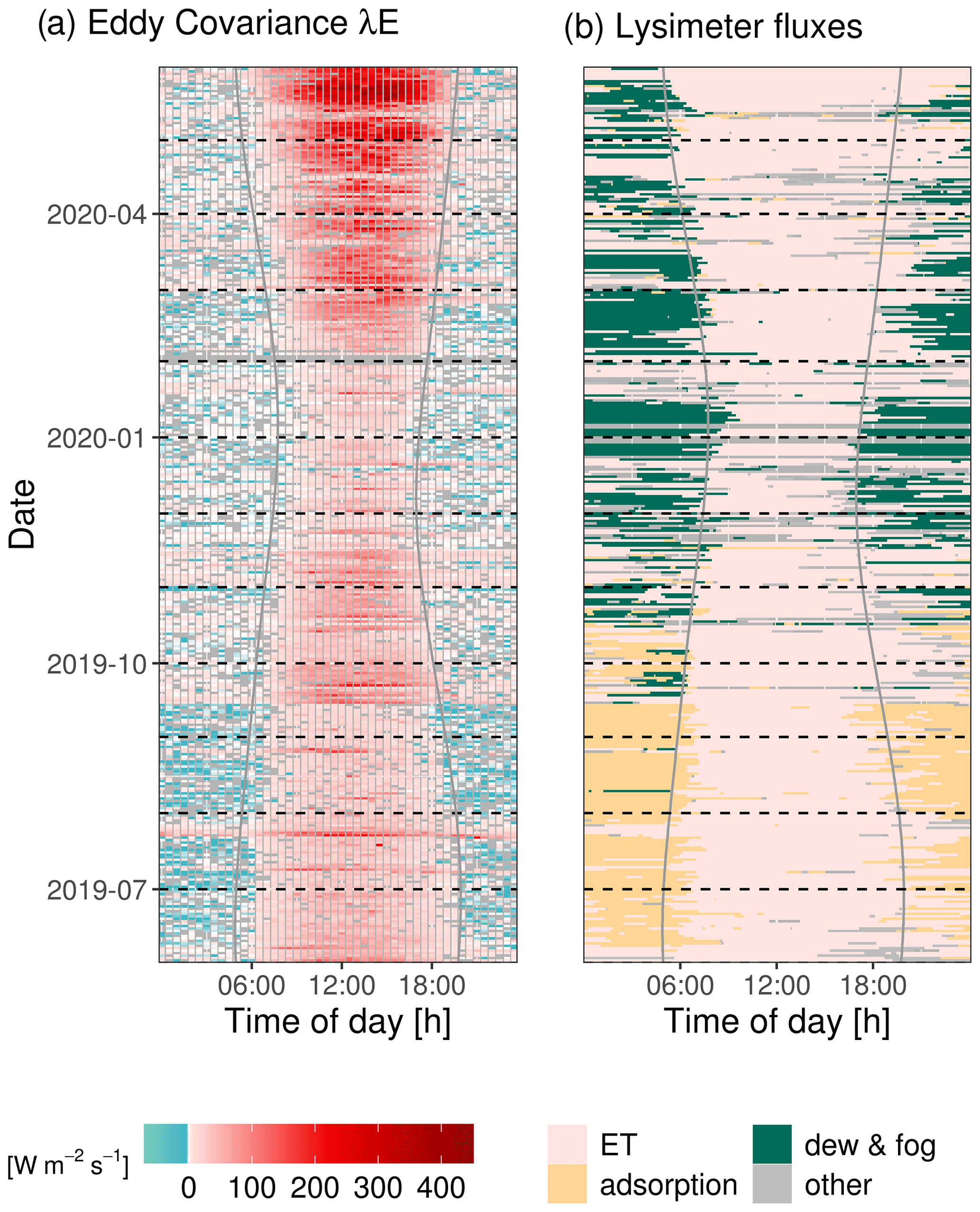
Figure 7Diel and seasonal variation in (a) quality-filtered λE fluxes from EC and (b) assigned lysimeter fluxes. Solid curved vertical lines mark sunrise and sunset, respectively, as determined by the geographic coordinates of the field site.
Figure 7 underpins results from Florentin and Agam (2017), who compared λE fluxes from EC and micro-lysimeters in the Negev in the dry season and found that EC was able to detect the dynamics, but not the magnitude, of adsorption from atmospheric humidity. Their study, however, covered only a period of 7 d. Previous research in a pine forest in Israel also indicated that EC-derived λE tends to be negative at night during adsorption (Qubaja et al., 2020).
More research in paired lysimeter EC setups is necessary to scientifically assess the suitability and limitations of EC-derived nighttime λE to detect and quantify the adsorption of atmospheric vapor on soil material. If found suitable, then EC instruments would help to spatially and temporally scale up the NRW research. Additionally, they could help to clarify the role of NRW across research communities (Gerlein-Safdi, 2021), for example, concerning the energy balance closure of EC (de Roode et al., 2010), ecological significance of foliar water uptake (Berry et al., 2019), and impacts on remote sensing products (Xu et al., 2021). Irrespectively, our findings underline the necessity for methods measuring processes of the water cycle during the night to avoid biased measurements towards evaporation while missing condensation.
In this work, we derive NRW from time series of automated weighted lysimeters and compare their length of occurrence with established model estimations. In summary, our data suggest that this semi-arid savanna ecosystem switches between evaporation and condensation almost daily. Attributing the condensation pattern to different NRW fluxes sheds light on the distinct mechanisms that are each dominant in a different season. In summer, the adsorption of atmospheric vapor on soil particles is facilitated by large diel temperature differences, and dry soils lead to steep gradients of atmospheric vapor pressure between the atmosphere and the soil air driving vapor diffusion. In winter and spring, high RH leads to frequent fog deposition and surface cooling to dew condensation. The spatial heterogeneity of vegetation, soil characteristics, and radiation regimes together with measurement uncertainties are more strongly reflected in NRW inputs than in other fluxes of surface water exchange. Although, between 1 June 2019 and 31 May 2020, the total NRW input sum comprises only 7.4 % of the local water input, the relative contribution strongly varies weekly. Rain frequency is unevenly distributed within the year, and especially atmospheric adsorption stands out as the only water input during 11 weeks in the dry season. The ecological relevance of these fluxes has yet to be scrutinized. Until a quantitative validation has been carried out for NRW from large weighing lysimeters, the measured sums should be interpreted with caution. Ideally, such validation would take the form of several campaigns with manual sampling of soil and plants throughout the year to cover the seasonally varying NRW fluxes.
Our analysis focuses on lysimeters that cover only a spatial area of 1 m2 each. We show that the temporal variability in the NRW derived from the instruments is coherent with negative λE fluxes at dry conditions. Based on this observation, future work could focus on reevaluating nighttime λE fluxes from EC instruments to improve the spatial representativeness and assess the relevance of NRW at a larger scale and across seasonally dry ecosystems.
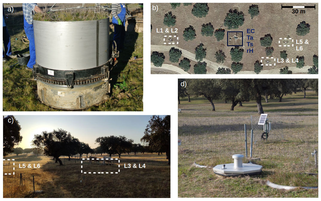
Figure A1Pictures of an (a) intact, vegetated soil monolith in the lysimeter vessel after excavation for installation in 2015 (picture by Oscar Perez-Priego). (b) Aerial view of the measurement setup, with the lysimeter stations marked by white rectangles and the EC and meteorological sensors marked by dark blue rectangles (map data from Google Earth; image from Instituto Geográfico Nacional). (c) Exemplar image of the site on 26 September at 08:30 LT in the morning to illustrate the heterogeneous shading conditions caused by the singular standing trees. (d) Lysimeter column 3 on 3 March 2022. The low fence around the station is installed to allow grazing of cows on the column, keeping them comparable with herbaceous vegetation outside the lysimeters, while reducing the risk of cows stepping on them (picture by Gerardo Moreno).
-
Surface temperature (Ts, ∘C) was calculated from measurements of the radiometric tower, as follows:
where LW is upwelling (↑) and downwelling (↓) longwave radiation (W m−2 s−1), ρ is the Boltzmann constant (W K−4 m−2), and ε is the emissivity of grass (–).
-
Dew point temperature (Tdew, ∘C) was calculated from RH and Ta, based on the Magnus equation (λ=17.62, β=243.12), as follows (Sonntag, 1990):
where RH is relative humidity (%), and Ta is air temperature (∘C).
-
Equations for evaluation statistics were used to compare measured (y) and modeled () duration lengths of dew and adsorption, respectively. n is the number of observations, and my and correspond to the means of y and , respectively.
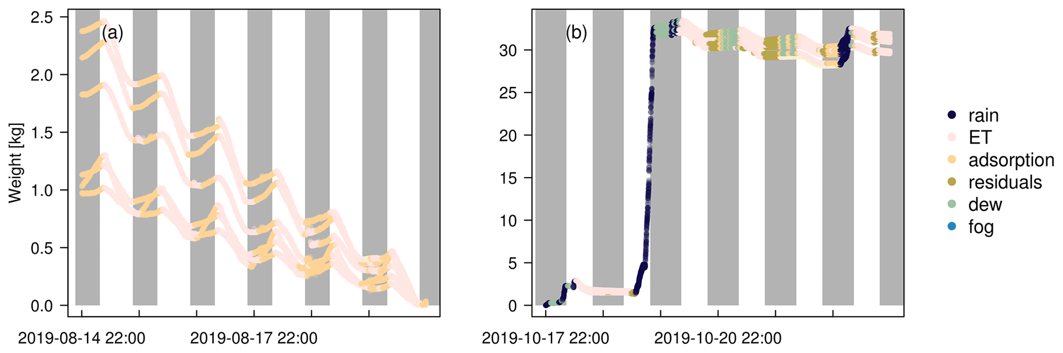
Figure D1Lysimeter weight (normalized over the shown time period for each lysimeter by subtracting the respective minimum weight) exemplar shown for (a) a week without rain from 15 to 20 August 2019 and (b) a week with several rain events from 18 to 23 October 2019. The color code shows the respective flux that was assigned to the preceding weight change. Gray shaded areas illustrate nights.
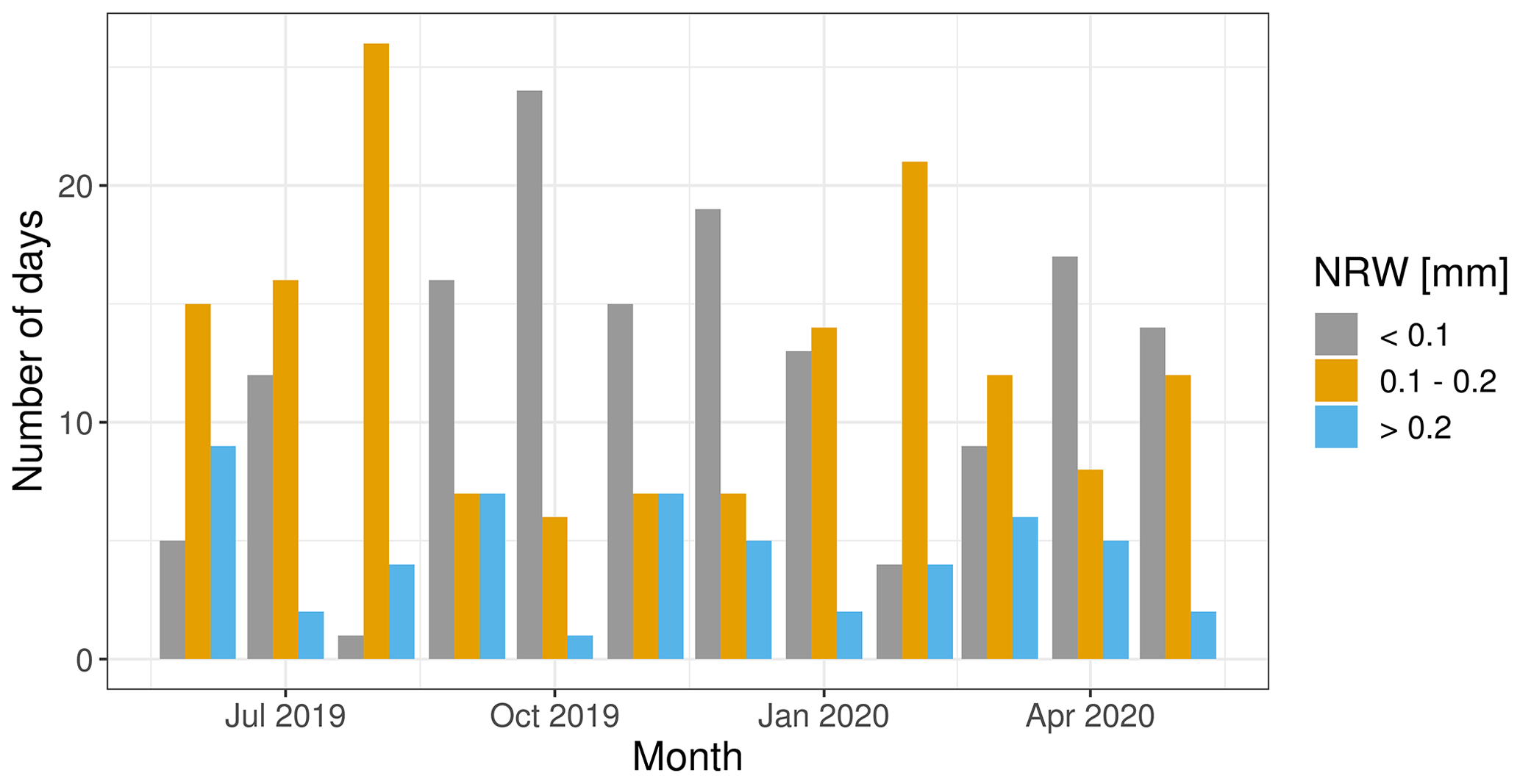
Figure E1The number of days per month with average NRW inputs of < 0.1, 0.1–0.2, and >0.2 mm d−1.
Table F1Evaluation statistics for the comparison of the occurrence duration between lysimeter measurements and modeling. Dew was modeled based on Penman–Monteith (PM), and the equilibrium evaporation model and adsorption were based on the aerodynamic diffusion equation. Statistics are shown for the options of (i) more than one and (ii) more than two lysimeters measuring dew or adsorption, respectively.
Suspended droplets during fog cause an optically thick layer that obstructs the surface radiation to the sky and creates a radiation equilibrium. Under such conditions, visibility sensors would also record a decrease in visibility which has been used in other studies, in addition to RH sensors, to separate fog from dew (e.g., Feigenwinter et al., 2020; Riedl et al., 2022). We visually identified mornings with fog and mornings where no fog occurred from images collected by a digital camera installed at the site from 1 October to 31 December 2020 between 06:00 and 14:30 LT. A direct comparison between the camera images and the lysimeter-measured fog deposition was not possible because fog could only be visually identified from pictures after sunrise. The deposition recorded with the lysimeters, however, stopped with sunrise. Lysimeter ΔW are exemplars shown with measurements of RH at different sensor heights and longwave radiation measurements in Fig. G1. Similar to measurements with a visibility sensor, fog should create a detectable radiation equilibrium at our sensor at 1.6 m measurement height. The hypothesis was tested by comparing the ratio of LW↑ to LW↓ between foggy and non-foggy conditions identified from the digital camera with the non-parametric Mann–Whitney U test.
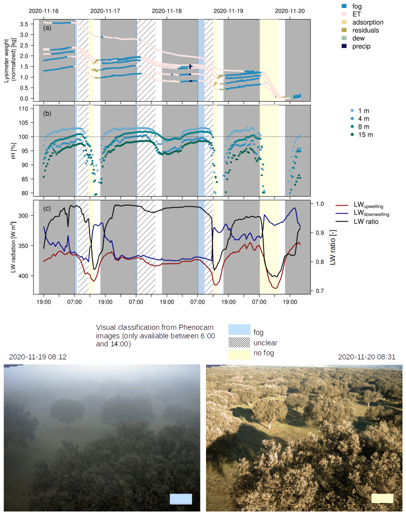
Figure G1Time series of (a) normalized weight changes in each lysimeter column with the respective assigned fluxes, (b) rH measurements, and (c) LW upwelling and LW downwelling and their respective ratios. Shaded areas illustrate nights (gray), conditions clearly identified as fog from digital camera images (blue; image bottom left), and non-foggy conditions (yellow; image bottom right). Hatched areas are used for periods that could not be unequivocally identified as foggy.
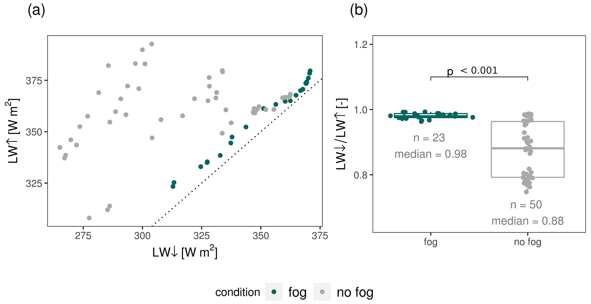
Figure G2Comparison of LW upwelling (↑) and LW downwelling (↓) during the conditions classified as having fog and without fog from a digital camera (example pictures shown in Fig. G1). The black dotted line in panel (a) displays the identity line. Panel (b) illustrates the radiation ratios during foggy and non-foggy conditions. The differences between the ratios are statistically significant, with a significance level of p<0.001.
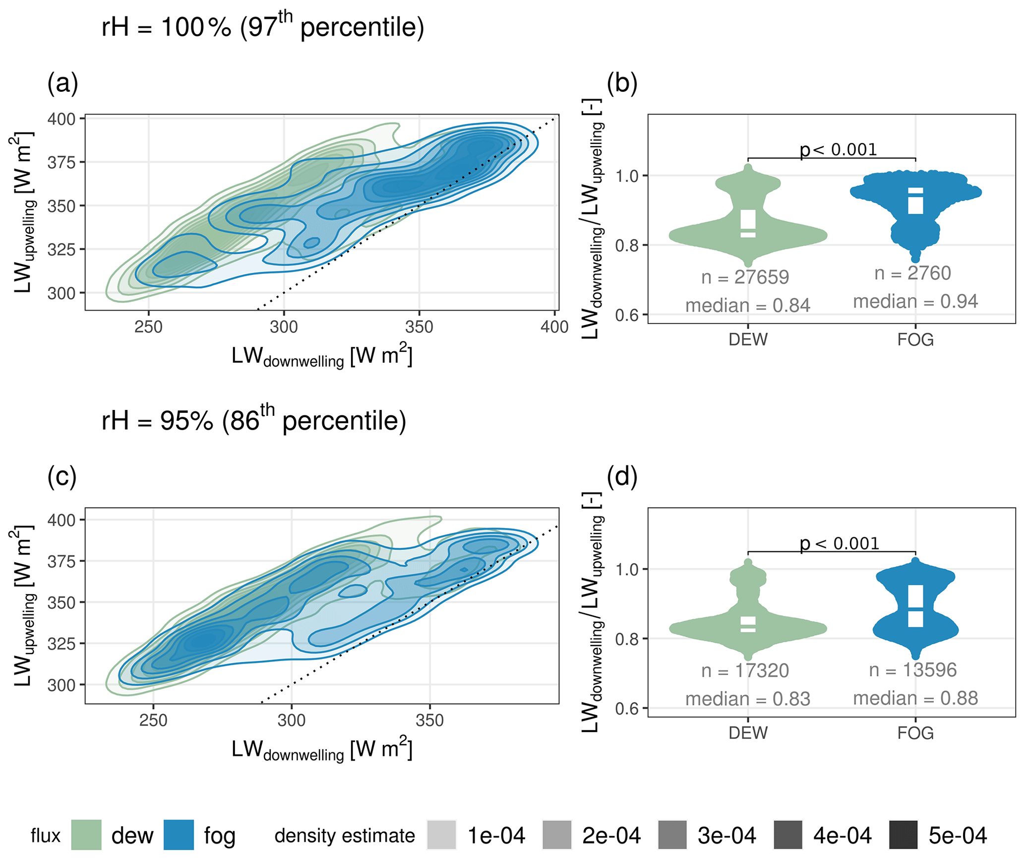
Figure G3Comparison of upwelling LW and downwelling LW during the conditions classified as having fog and dew from the flux partitioning of the lysimeter weight changes based on a rH threshold of 100 % (a, b) and 95 % (c, d). Panels (a) and (c) illustrate the smoothed kernel density estimate, with the black dotted line displaying the identity line. Panels (b) and (d) illustrate the distribution of radiation ratios during dew and fog conditions. The differences between the distributions are statistically significant, with a significance level p<0.001.
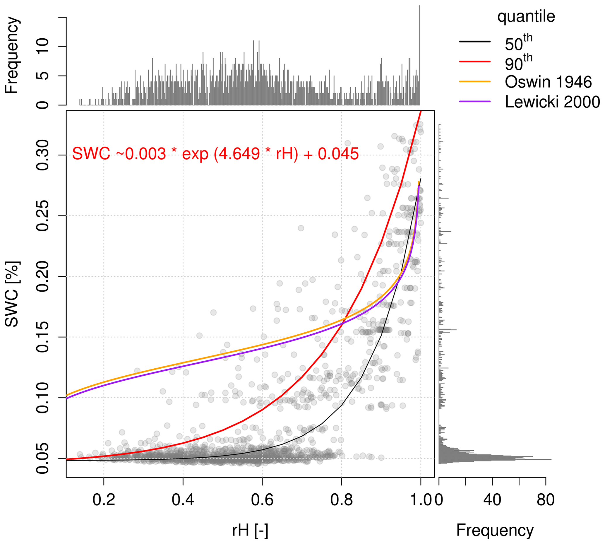
Figure H1Relationship of SWC and rH during modeled adsorption (gradient-driven vapor diffusion towards the soil surface) from April to October. The full formula with the parameters for the 90th quantile from nonlinear quantile regression is given in the upper left. The black line additionally illustrates the 50th quantile. Empirical relationships from the literature for equilibrated conditions are shown in orange and purple (Oswin, 1946; Lewicki, 2000).
Data and the R code to reproduce the results of this analysis are available in Paulus et al. (2022) at https://doi.org/10.5281/zenodo.7354493.
MM, RO, MR, OPP, and SP designed the setup and planned the study. OK, GM, AC, TEM, MM, and OPP maintained the site and instrumentation and conducted the measurements. SP, TEM, and TW processed the data. SP analyzed the data and prepared the original draft, both under the supervision of MM, RO, TEM, and AH. All authors discussed, reviewed, and edited the paper.
The contact author has declared that none of the authors has any competing interests.
Publisher's note: Copernicus Publications remains neutral with regard to jurisdictional claims in published maps and institutional affiliations.
We thank the city council of Majadas de Tiétar, for support. Our thanks go to Martin Strube, Ramón López-Jimenez, Martin Hertel, and the Freiland group at the MPI-BGC, for great technical and scientific assistance during fieldwork. Sinikka Jasmin Paulus would further like to thank Andre Peters and Johanna Böcher, for their helpful comments and suggestions. The authors acknowledge the Alexander von Humboldt Foundation, for supporting this research through the Max Planck Research Prize 2013 to Markus Reichstein. We thank Werner Eugster, Giora J. Kidron, and Xiaohong Jia, for their valuable comments on earlier drafts of the paper.
Sinikka Jasmin Paulus has been supported by funding through the International Max Planck Research School for Global Biogeochemical Cycles (IMPRS-gBGC) at the University of Jena. René Orth has been supported by funding from the German Research Foundation (Emmy Noether Grant; grant no. 391059971). The Alexander von Humboldt Foundation has supported this research through the Max Planck Research Prize 2013 to Markus Reichstein.
The article processing charges for this open-access publication were covered by the Max Planck Society.
This paper was edited by Lixin Wang and reviewed by Werner Eugster, Xiaohong Jia, and Giora J. Kidron.
Agam, N. and Berliner, P.: Dew formation and water vapor adsorption in semi-arid environments – A review, J. Arid Environ., 65, 572–590, https://doi.org/10.1016/j.jaridenv.2005.09.004, 2006. a
Aguirre-Gutiérrez, C. A., Holwerda, F., Goldsmith, G. R., Delgado, J., Yepez, E., Carbajal, N., Escoto-Rodríguez, M., and Arredondo, J. T.: The importance of dew in the water balance of a continental semiarid grassland, J. Arid Environ., 168, 26–35, https://doi.org/10.1016/j.jaridenv.2019.05.003, 2019. a
Aparecido, L. M. T., Miller, G. R., Cahill, A. T., and Moore, G. W.: Leaf surface traits and water storage retention affect photosynthetic responses to leaf surface wetness among wet tropical forest and semiarid savanna plants, Tree Physiol., 37, 1285–1300, https://doi.org/10.1093/treephys/tpx092, 2017. a, b
Arthur, E., Tuller, M., Moldrup, P., and de Jonge, L. W.: Evaluation of theoretical and empirical water vapor sorption isotherm models for soils, Water Resour. Res., 52, 190–205, https://doi.org/10.1002/2015WR017681, 2016. a, b, c
Baldocchi, D.: Measuring fluxes of trace gases and energy between ecosystems and the atmosphere – the state and future of the eddy covariance method, Global Change Biol., 20, 3600–3609, https://doi.org/10.1111/gcb.12649, 2014. a
Baldocchi, D. D.: How eddy covariance flux measurements have contributed to our understanding of Global Change Biology, Global Change Biol., 26, 242–260, https://doi.org/10.1111/gcb.14807, 2020. a
Ben-Asher, J., Alpert, P., and Ben-Zvi, A.: Dew is a major factor affecting vegetation water use efficiency rather than a source of water in the eastern Mediterranean area, Water Resour. Res., 46, 2008WR007484, https://doi.org/10.1029/2008WR007484, 2010. a
Berry, Z. C., White, J. C., and Smith, W. K.: Foliar uptake, carbon fluxes and water status are affected by the timing of daily fog in saplings from a threatened cloud forest, Tree Physiol., 34, 459–470, https://doi.org/10.1093/treephys/tpu032, 2014. a
Berry, Z. C., Emery, N. C., Gotsch, S. G., and Goldsmith, G. R.: Foliar water uptake: Processes, pathways, and integration into plant water budgets: Foliar Water Uptake, Plant Cell Environ., 42, 410–423, https://doi.org/10.1111/pce.13439, 2019. a, b
Beysens, D.: Dew water, River Publishers, https://doi.org/10.1201/9781003337898, 2018. a
Bogdanovich, E., Perez-Priego, O., El-Madany, T. S., Guderle, M., Pacheco-Labrador, J., Levick, S. R., Moreno, G., Carrara, A., Pilar Martín, M., and Migliavacca, M.: Using terrestrial laser scanning for characterizing tree structural parameters and their changes under different management in a Mediterranean open woodland, Forest Ecol. Manage., 486, 118945, https://doi.org/10.1016/j.foreco.2021.118945, 2021. a, b
Camuffo, D.: Condensation-evaporation cycles in pore and capillary systems according to the Kelvin model, Water Air Soil Poll., 21, 151–159, https://doi.org/10.1007/BF00163620, 1984. a
Dawson, T. E. and Goldsmith, G. R.: The value of wet leaves, New Phytol., 219, 1156–1169, https://doi.org/10.1111/nph.15307, 2018. a, b, c, d, e
de Roode, S. R., Bosveld, F. C., and Kroon, P. S.: Dew Formation, Eddy-Correlation Latent Heat Fluxes, and the Surface Energy Imbalance at Cabauw During Stable Conditions, Bound.-Lay. Meteorol., 135, 369–383, https://doi.org/10.1007/s10546-010-9476-1, 2010. a
Dijkema, J., Koonce, J., Shillito, R., Ghezzehei, T., Berli, M., van der Ploeg, M., and van Genuchten, M.: Water Distribution in an Arid Zone Soil: Numerical Analysis of Data from a Large Weighing Lysimeter, Vadose Zone J., 17, 1–17, https://doi.org/10.2136/vzj2017.01.0035, 2018. a
Dirks, I., Navon, Y., Kanas, D., Dumbur, R., and Grünzweig, J. M.: Atmospheric water vapor as driver of litter decomposition in Mediterranean shrubland and grassland during rainless seasons, Global Change Biol., 16, 2799–2812, https://doi.org/10.1111/j.1365-2486.2010.02172.x, 2010. a
Duvdevani, S.: Dew in Israel and its effect on plants, Soil Sci., 98, 14–21, 1964. a
Edlefsen, N. and Anderson, A.: Thermodynamics of soil moisture, Hilgardia, 15, 31–298, https://doi.org/10.3733/hilg.v15n02p031, 1943. a
El-Madany, T. S., Reichstein, M., Perez-Priego, O., Carrara, A., Moreno, G., Pilar Martín, M., Pacheco-Labrador, J., Wohlfahrt, G., Nieto, H., Weber, U., Kolle, O., Luo, Y.-P., Carvalhais, N., and Migliavacca, M.: Drivers of spatio-temporal variability of carbon dioxide and energy fluxes in a Mediterranean savanna ecosystem, Agr. Forest Meteorol., 262, 258–278, https://doi.org/10.1016/j.agrformet.2018.07.010, 2018. a, b
El-Madany, T. S., Carrara, A., Martín, M. P., Moreno, G., Kolle, O., Pacheco-Labrador, J., Weber, U., Wutzler, T., Reichstein, M., and Migliavacca, M.: Drought and heatwave impacts on semi-arid ecosystems' carbon fluxes along a precipitation gradient, Philos. T. Roy. Soc. B, 375, 20190519, https://doi.org/10.1098/rstb.2019.0519, 2020. a
El-Madany, T. S., Reichstein, M., Carrara, A., Martín, M. P., Moreno, G., Gonzalez-Cascon, R., Peñuelas, J., Ellsworth, D. S., Burchard-Levine, V., Hammer, T. W., Knauer, J., Kolle, O., Luo, Y., Pacheco-Labrador, J., Nelson, J. A., Perez-Priego, O., Rolo, V., Wutzler, T., and Migliavacca, M.: How Nitrogen and Phosphorus Availability Change Water Use Efficiency in a Mediterranean Savanna Ecosystem, J. Geophys. Res.-Biogeo., 126, e2020JG006005, https://doi.org/10.1029/2020JG006005, 2021. a, b
Evans, S., Todd-Brown, K. E. O., Jacobson, K., and Jacobson, P.: Non-rainfall Moisture: A Key Driver of Microbial Respiration from Standing Litter in Arid, Semiarid, and Mesic Grasslands, Ecosystems, 23, 1154–1169, https://doi.org/10.1007/s10021-019-00461-y, 2019. a, b
Feigenwinter, C., Franceschi, J., Larsen, J. A., Spirig, R., and Vogt, R.: On the performance of microlysimeters to measure non-rainfall water input in a hyper-arid environment with focus on fog contribution, J. Arid Environ., 182, 104260, https://doi.org/10.1016/j.jaridenv.2020.104260, 2020. a, b, c, d, e, f, g, h
Fernández, V., Sancho-Knapik, D., Guzmán, P., Peguero-Pina, J. J., Gil, L., Karabourniotis, G., Khayet, M., Fasseas, C., Heredia-Guerrero, J. A., Heredia, A., and Gil-Pelegrín, E.: Wettability, Polarity, and Water Absorption of Holm Oak Leaves: Effect of Leaf Side and Age, Plant Physiol., 166, 168–180, https://doi.org/10.1104/pp.114.242040, 2014. a
Florentin, A. and Agam, N.: Estimating non-rainfall-water-inputs-derived latent heat flux with turbulence-based methods, Agr. Forest Meteorol., 247, 533–540, https://doi.org/10.1016/j.agrformet.2017.08.035, 2017. a, b
Gerlein-Safdi, C.: Seeing dew deposition from satellites: leveraging microwave remote sensing for the study of water dynamics in and on plants, New Phytol., 231, 5–7, https://doi.org/10.1111/nph.17418, 2021. a
Gerlein-Safdi, C., Gauthier, P. P. G., and Caylor, K. K.: Dew-induced transpiration suppression impacts the water and isotope balances of Colocasia leaves, Oecologia, 187, 1041–1051, https://doi.org/10.1007/s00442-018-4199-y, 2018. a
Glickman, T. S. and Zenk, W.: Glossary of Meteorology, 2nd Edn., AMS – American Meteorological Society, Boston, MA, https://glossary.ametsoc.org/wiki/Fog (last access: 9 December 2022), 2000. a
Gliksman, D., Rey, A., Seligmann, R., Dumbur, R., Sperling, O., Navon, Y., Haenel, S., De Angelis, P., Arnone, J. A., and Grüzweig, J. M.: Biotic degradation at night, abiotic degradation at day: positive feedbacks on litter decomposition in drylands, Global Change Biol., 23, 1564–1574, https://doi.org/10.1111/gcb.13465, 2017. a, b
Göckede, M., Rebmann, C., and Foken, T.: A combination of quality assessment tools for eddy covariance measurements with footprint modelling for the characterisation of complex sites, Agr. Forest Meteorol., 127, 175–188, https://doi.org/10.1016/j.agrformet.2004.07.012, 2004. a
Groh, J., Vanderborght, J., Pütz, T., and Vereecken, H.: How to Control the Lysimeter Bottom Boundary to Investigate the Effect of Climate Change on Soil Processes?, Vadose Zone J., 15, vzj2015.08.0113, https://doi.org/10.2136/vzj2015.08.0113, 2016. a, b
Groh, J., Slawitsch, V., Herndl, M., Graf, A., Vereecken, H., and Pütz, T.: Determining dew and hoar frost formation for a low mountain range and alpine grassland site by weighable lysimeter, J. Hydrol., 563, 372–381, https://doi.org/10.1016/j.jhydrol.2018.06.009, 2018. a, b, c, d, e
Hannes, M., Wollschläger, U., Schrader, F., Durner, W., Gebler, S., Pütz, T., Fank, J., von Unold, G., and Vogel, H.-J.: A comprehensive filtering scheme for high-resolution estimation of the water balance components from high-precision lysimeters, Hydrol. Earth Syst. Sci., 19, 3405–3418, https://doi.org/10.5194/hess-19-3405-2015, 2015. a, b, c, d
Hill, A. J., Dawson, T. E., Shelef, O., and Rachmilevitch, S.: The role of dew in Negev Desert plants, Oecologia, 178, 317–327, https://doi.org/10.1007/s00442-015-3287-5, 2015. a
IUSS Working Group WRB: World reference base for soil resources 2014: International soil classification system for naming soils and creating legends for soil maps, Update 2015, https://www.fao.org/3/i3794en/I3794en.pdf (last access: 9 December 2022), 2014. a
Jacobs, A. F. G., Heusinkveld, B. G., Wichink Kruit, R. J., and Berkowicz, S. M.: Contribution of dew to the water budget of a grassland area in the Netherlands, Water Resour. Res., 42, W03415, https://doi.org/10.1029/2005WR004055, 2006. a, b, c
Jung, M., Reichstein, M., Ciais, P., Seneviratne, S. I., Sheffield, J., Goulden, M. L., Bonan, G., Cescatti, A., Chen, J., de Jeu, R., Dolman, A. J., Eugster, W., Gerten, D., Gianelle, D., Gobron, N., Heinke, J., Kimball, J., Law, B. E., Montagnani, L., Mu, Q., Mueller, B., Oleson, K., Papale, D., Richardson, A. D., Roupsard, O., Running, S., Tomelleri, E., Viovy, N., Weber, U., Williams, C., Wood, E., Zaehle, S., and Zhang, K.: Recent decline in the global land evapotranspiration trend due to limited moisture supply, Nature, 467, 951–954, https://doi.org/10.1038/nature09396, 2010. a
Kidron, G. J.: The effect of substrate properties, size, position, sheltering and shading on dew: An experimental approach in the Negev Desert, Atmos. Res., 98, 378–386, https://doi.org/10.1016/j.atmosres.2010.07.015, 2010. a
Kidron, G. J. and Kronenfeld, R.: Atmospheric humidity is unlikely to serve as an important water source for crustose soil lichens in the Tabernas Desert, J. Hydrol. Hydromech., 68, 359–367, https://doi.org/10.2478/johh-2020-0034, 2020a. a, b, c, d
Kidron, G. J. and Kronenfeld, R.: Microlysimeters overestimate the amount of non-rainfall water – an experimental approach, Catena, 194, 104691, https://doi.org/10.1016/j.catena.2020.104691, 2020b. a, b, c
Kidron, G. J. and Lázaro, R.: Are coastal deserts necessarily dew deserts? An example from the Tabernas Desert, J. Hydrol. Hydromech., 68, 19–27, https://doi.org/10.2478/johh-2020-0002, 2020. a
Kidron, G. J. and Starinsky, A.: Measurements and ecological implications of non-rainfall water in desert ecosystem – A review, Ecohydrology, 12, e2121, https://doi.org/10.1002/eco.2121, 2019. a, b, c, d, e
Kidron, G. J., Yair, A., and Danin, A.: Dew variability within a small arid drainage basin in the Negev Highlands, Israel, Q. J. Roy. Meteorol. Soc., 126, 63–80, https://doi.org/10.1002/qj.49712656204, 2000. a
Knauer, J., El-Madany, T. S., Zaehle, S., and Migliavacca, M.: Bigleaf – An R package for the calculation of physical and physiological ecosystem properties from eddy covariance data, PLOS ONE, 13, e0201114, https://doi.org/10.1371/journal.pone.0201114, 2018. a
Kohfahl, C., Molano-Leno, L., Marínez, G., Vanderlinden, K., Guardiola-Albert, C., and Moreno, L.: Determining groundwater recharge and vapor flow in dune sediments using a weighable precision meteo lysimeter, Sci. Total Environ., 656, 550–557, https://doi.org/10.1016/j.scitotenv.2018.11.415, 2019. a, b
Kosmas, C., Danalatos, N., Poesen, J., and van Wesemael, B.: The effect of water vapour adsorption on soil moisture content under Mediterranean climatic conditions, Agr. Water Manage., 36, 157–168, https://doi.org/10.1016/S0378-3774(97)00050-4, 1998. a
Kosmas, C., Marathianou, M., Gerontidis, S., Detsis, V., Tsara, M., and Poesen, J.: Parameters affecting water vapor adsorption by the soil under semi-arid climatic conditions, Agr. Water Manage., 48, 61–78, https://doi.org/10.1016/S0378-3774(00)00113-X, 2001. a, b, c, d
Lewicki, P. P.: Raoult's law based food water sorption isotherm, J. Food Eng., 43, 31–40, 2000. a
Li, S., Xiao, B., Sun, F., and Kidron, G. J.: Moss-dominated biocrusts enhance water vapor sorption capacity of surface soil and increase non-rainfall water deposition in drylands, Geoderma, 388, 114930, https://doi.org/10.1016/j.geoderma.2021.114930, 2021. a
Li, Y., Aemisegger, F., Riedl, A., Buchmann, N., and Eugster, W.: The role of dew and radiation fog inputs in the local water cycling of a temperate grassland during dry spells in central Europe, Hydrol. Earth Syst. Sci., 25, 2617–2648, https://doi.org/10.5194/hess-25-2617-2021, 2021. a, b, c, d, e, f
Lopez-Canfin, C., Lázaro, R., and Sánchez-Cañete, E. P.: Disparate responses of soil-atmosphere CO2 exchange to biophysical and geochemical factors over a biocrust ecological succession in the Tabernas Desert, Geoderma, 425, 116067, https://doi.org/10.1016/j.geoderma.2022.116067, 2022. a
López-Ballesteros, A., Serrano-Ortiz, P., Sánchez-Cañete, E. P., Oyonarte, C., Kowalski, A. S., Pérez-Priego, Ã., and Domingo, F.: Enhancement of the net CO2 release of a semiarid grassland in SE Spain by rain pulses, J. Geophys. Res., 121, 52–66, https://doi.org/10.1002/2015JG003091, 2016. a
Luo, Y., El-Madany, T., Ma, X., Nair, R., Jung, M., Weber, U., Filippa, G., Bucher, S. F., Moreno, G., Cremonese, E., Carrara, A., Gonzalez-Cascon, R., Cáceres Escudero, Y., Galvagno, M., Pacheco-Labrador, J., Martín, M. P., Perez-Priego, O., Reichstein, M., Richardson, A. D., Menzel, A., Römermann, C., and Migliavacca, M.: Nutrients and water availability constrain the seasonality of vegetation activity in a Mediterranean ecosystem, Global Change Biol., 26, 4379–4400, https://doi.org/10.1111/gcb.15138, 2020. a
Massman, W. and Lee, X.: Eddy covariance flux corrections and uncertainties in long-term studies of carbon and energy exchanges, Agr. Forest Meteorol., 113, 121–144, https://doi.org/10.1016/S0168-1923(02)00105-3, 2002. a
McHugh, T. A., Morrissey, E. M., Reed, S. C., Hungate, B. A., and Schwartz, E.: Water from air: an overlooked source of moisture in arid and semiarid regions, Scient. Rep., 5, 13767, https://doi.org/10.1038/srep13767, 2015. a, b
Meissner, R., Rupp, H., and Schubert, M.: Novel lysimeter techniques' basis for the improved investigation of water, gas, and solute transport in soils, J. Plant Nutr. Soil Sci., 163, 603–608, 2000. a
Meissner, R., Seeger, J., Rupp, H., Seyfarth, M., and Borg, H.: Measurement of dew, fog, and rime with a high-precision gravitation lysimeter, J. Plant Nutr. Soil Sci., 170, 335–344, https://doi.org/10.1002/jpln.200625002, 2007. a
Migliavacca, M., Perez-Priego, O., Rossini, M., El-Madany, T. S., Moreno, G., van der Tol, C., Rascher, U., Berninger, A., Bessenbacher, V., Burkart, A., Carrara, A., Fava, F., Guan, J.-H., Hammer, T. W., Henkel, K., Juarez-Alcalde, E., Julitta, T., Kolle, O., Martín, M. P., Musavi, T., Pacheco-Labrador, J., Pérez-Burgueño, A., Wutzler, T., Zaehle, S., and Reichstein, M.: Plant functional traits and canopy structure control the relationship between photosynthetic CO2 uptake and far-red sun-induced fluorescence in a Mediterranean grassland under different nutrient availability, New Phytol., 214, 1078–1091, https://doi.org/10.1111/nph.14437, 2017. a, b, c, d
Milly, P.: A simulation analysis of thermal effects on evaporation from soil, Water Resour. Res., 20, 1087–1098, 1984. a
Monteith, J. L.: Dew, Q. J. Roy. Meteorol. Soc., 83, 322–341, https://doi.org/10.1002/qj.49708335706, 1957. a, b
Monteith, J. L.: Evaporation and environment. The stage and movement of water in living organisms, in: Symposia of the Society for Experimental Biology, vol. 19, Cambridge University Press, 205–234, PMID 5321565, 1965. a
Monteith, J. L. and Unsworth, M. H.: Principles of environmental physics: plants, animals, and the atmosphere, in: 4th Edn., oCLC: ocn858967864, Elsevier/Academic Press, Amsterdam, Boston, Hardcover ISBN 9780123869104, eBook ISBN 9780123869937, 2013. a
Nair, R. K. F., Morris, K. A., Hertel, M., Luo, Y., Moreno, G., Reichstein, M., Schrumpf, M., and Migliavacca, M.: N:P stoichiometry and habitat effects on Mediterranean savanna seasonal root dynamics, Biogeosciences, 16, 1883–1901, https://doi.org/10.5194/bg-16-1883-2019, 2019. a, b
Nolz, R., Kammerer, G., and Cepuder, P.: Interpretation of lysimeter weighing data affected by wind, J. Plant Nutr. Soil Sci., 176, 200–208, https://doi.org/10.1002/jpln.201200342, 2013. a, b
Nolz, R., Cepuder, P., and Kammerer, G.: Determining soil water-balance components using an irrigated grass lysimeter in NE Austria, J. Plant Nutr. Soil Sci., 177, 237–244, https://doi.org/10.1002/jpln.201300335, 2014. a
Orchiston, H. D.: Adsorption of water vapor: I. Soils at 25 ∘C, Soil Sci., 76, 453–466, https://doi.org/10.1097/00010694-195312000-00005, 1953. a
Oswin, C. R.: The kinetics of package life. III. The isotherm, J. Soc. Chem. Indust., 65, 419–421, https://doi.org/10.1002/jctb.5000651216, 1946. a
Panwar, A., Kleidon, A., and Renner, M.: Do Surface and Air Temperatures Contain Similar Imprints of Evaporative Conditions?, Geophys. Res. Lett., 46, 3802–3809, https://doi.org/10.1029/2019GL082248, 2019. a
Paulus, S. J., El-Madany, T. S., Wutzler, T., Carrara, A., Moreno, G. M., Reichstein, M., Orth, R., Hertel, M., López-Jimenez, R., and Migliavacca, M.: High-resolution large weighing lysimeter measurements with meteorological and soil- hydrological variables from a Mediterranean Savanna, Zenodo [code and data set], https://doi.org/10.5281/zenodo.7354493, 2022. a
Perez-Priego, O., El-Madany, T. S., Migliavacca, M., Kowalski, A. S., Jung, M., Carrara, A., Kolle, O., Martín, M. P., Pacheco-Labrador, J., Moreno, G., and Reichstein, M.: Evaluation of eddy covariance latent heat fluxes with independent lysimeter and sapflow estimates in a Mediterranean savannah ecosystem, Agr. Forest Meteorol., 236, 87–99, https://doi.org/10.1016/j.agrformet.2017.01.009, 2017. a, b, c
Perez-Priego, O., Katul, G., Reichstein, M., El-Madany, T. S., Ahrens, B., Carrara, A., Scanlon, T. M., and Migliavacca, M.: Partitioning Eddy Covariance Water Flux Components Using Physiological and Micrometeorological Approaches, J. Geophys. Res.-Biogeo., 123, 3353–3370, https://doi.org/10.1029/2018JG004637, 2018. a, b
Peters, A., Nehls, T., Schonsky, H., and Wessolek, G.: Separating precipitation and evapotranspiration from noise – a new filter routine for high-resolution lysimeter data, Hydrol. Earth Syst. Sci., 18, 1189–1198, https://doi.org/10.5194/hess-18-1189-2014, 2014. a, b
Peters, A., Nehls, T., and Wessolek, G.: Technical note: Improving the AWAT filter with interpolation schemes for advanced processing of high resolution data, Hydrol. Earth Syst. Sci., 20, 2309–2315, https://doi.org/10.5194/hess-20-2309-2016, 2016. a, b
Peters, A., Groh, J., Schrader, F., Durner, W., Vereecken, H., and Pütz, T.: Towards an unbiased filter routine to determine precipitation and evapotranspiration from high precision lysimeter measurements, J. Hydrol., 549, 731–740, https://doi.org/10.1016/j.jhydrol.2017.04.015, 2017. a, b, c, d
Podlasly, C. and Schwärzel, K.: Development of a Continuous Closed Pipe System for Controlling SoilTemperature at the Lower Boundary of Weighing Field Lysimeters, Soil Sci. Soc. Am. J., 77, 2157–2163, https://doi.org/10.2136/sssaj2013.03.0113n, 2013. a
Price, J. D. and Clark, R.: On the Measurement of Dewfall and Fog-Droplet Deposition, Bound.-Lay. Meteorol., 152, 367–393, https://doi.org/10.1007/s10546-014-9930-6, 2014. a, b
Qubaja, R., Amer, M., Tatarinov, F., Rotenberg, E., Preisler, Y., Sprintsin, M., and Yakir, D.: Partitioning evapotranspiration and its long-term evolution in a dry pine forest using measurement-based estimates of soil evaporation, Agr. Forest Meteorol., 281, 107831, https://doi.org/10.1016/j.agrformet.2019.107831, 2020. a, b, c
R Core Team: R: A Language and Environment for Statistical Computing, R Foundation for Statistical Computing, Vienna, Austria, https://www.R-project.org/ (last access: 9 December 2022), 2020. a
Reichstein, M., Papale, D., Valentini, R., Aubinet, M., Bernhofer, C., Knohl, A., Laurila, T., Lindroth, A., Moors, E., Pilegaard, K., and Seufert, G.: Determinants of terrestrial ecosystem carbon balance inferred from European eddy covariance flux sites, Geophys. Res. Lett., 34, L01402, https://doi.org/10.1029/2006GL027880, 2007. a
Reth, S., Perez-Priego, O., Coners, H., and Nolz, R.: Lysimeter, Springer International Publishing, Cham, 1583–1593, https://doi.org/10.1007/978-3-030-52171-4_58, 2021. a
Riedl, A., Li, Y., Eugster, J., Buchmann, N., and Eugster, W.: Technical note: High-accuracy weighing micro-lysimeter system for long-term measurements of non-rainfall water inputs to grasslands, Hydrol. Earth Syst. Sci., 26, 91–116, https://doi.org/10.5194/hess-26-91-2022, 2022. a, b, c, d, e, f
Ritter, F., Berkelhammer, M., and Beysens, D.: Dew frequency across the US from a network of in situ radiometers, Hydrol. Earth Syst. Sci., 23, 1179–1197, https://doi.org/10.5194/hess-23-1179-2019, 2019. a, b
Rodriguez-Iturbe, I., Porporato, A., Laio, F., and Ridol, L.: Plants in water-controlled ecosystems: active role in hydrologic processes and response to water stress I. Scope and general outline, Adv. Water Resour., 24, 695–705, https://doi.org/10.1016/S0309-1708(01)00004-5, 2001. a
Saaltink, M. W., Kohfahl, C., and Molano-Leno, L.: Analysis of water vapor adsorption in soils by means of a lysimeter and numerical modeling, Vadose Zone J., 19, e20012, https://doi.org/10.1002/vzj2.20012, 2020. a, b, c
Schneider, J., Groh, J., Pütz, T., Helmig, R., Rothfuss, Y., Vereecken, H., and Vanderborght, J.: Prediction of soil evaporation measured with weighable lysimeters using the FAO Penman–Monteith method in combination with Richards' equation, Vadose Zone J., 20, e20102, https://doi.org/10.1002/vzj2.20102, 2021. a
Schrader, F., Durner, W., Fank, J., Gebler, S., Pütz, T., Hannes, M., and Wollschläger, U.: Estimating Precipitation and Actual Evapotranspiration from Precision Lysimeter Measurements, Proced. Environ. Sci., 19, 543–552, https://doi.org/10.1016/j.proenv.2013.06.061, 2013. a, b, c, d
Seneviratne, S. I., Corti, T., Davin, E. L., Hirschi, M., Jaeger, E. B., Lehner, I., Orlowsky, B., and Teuling, A. J.: Investigating soil moisture–climate interactions in a changing climate: A review, Earth-Sci. Rev., 99, 125–161, https://doi.org/10.1016/j.earscirev.2010.02.004, 2010. a
Sonntag, D.: Important new values of the physical constants of 1986, vapour pressure formulations based on the ITS-90, and psychrometer formulae, Z. Meteorol., 40, 340–344, 1990. a
Thom, A.: Momentum, mass and heat exchange of vegetation, Q. J. Roy. Meteorol. Soc., 98, 124–134, https://doi.org/10.1002/qj.49709841510, 1972. a
Tomaszkiewicz, M., Abou Najm, M., Beysens, D., Alameddine, I., and El-Fadel, M.: Dew as a sustainable non-conventional water resource: a critical review, Environ. Rev., 23, 425–442, https://doi.org/10.1139/er-2015-0035, 2015. a, b, c, d, e, f, g
Tuller, M., Or, D., and Dudley, L. M.: Adsorption and capillary condensation in porous media: Liquid retention and interfacial configurations in angular pores, Water Resour. Res., 35, 1949–1964, https://doi.org/10.1029/1999WR900098, 1999. a, b
Uclés, O., Villagarcía, L., Moro, M. J., Canton, Y., and Domingo, F.: Role of dewfall in the water balance of a semiarid coastal steppe ecosystem, Hydrol. Process., 28, 2271–2280, https://doi.org/10.1002/hyp.9780, 2014. a, b, c, d
Uclés, O., Villagarcía, L., Cantón, Y., Lázaro, R., and Domingo, F.: Non-rainfall water inputs are controlled by aspect in a semiarid ecosystem, J. Arid Environ., 113, 43–50, https://doi.org/10.1016/j.jaridenv.2014.09.009, 2015. a, b, c
Uclés, O., Villagarcía, L., Cantón, Y., and Domingo, F.: Partitioning of non rainfall water input regulated by soil cover type, Catena, 139, 265–270, https://doi.org/10.1016/j.catena.2015.02.018, 2016. a
Verhoef, A., Diaz-Espejo, A., Knight, J. R., Villagarcía, L., and Fernández, J. E.: Adsorption of Water Vapor by Bare Soil in an Olive Grove in Southern Spain, J. Hydrometeorol., 7, 1011–1027, https://doi.org/10.1175/JHM556.1, 2006. a, b, c, d, e, f
Wærsted, E. G., Haeffelin, M., Dupont, J.-C., Delanoë, J., and Dubuisson, P.: Radiation in fog: quantification of the impact on fog liquid water based on ground-based remote sensing, Atmos. Chem. Phys., 17, 10811–10835, https://doi.org/10.5194/acp-17-10811-2017, 2017. a, b
Weathers, K. C., Ponette-González, A. G., and Dawson, T. E.: Medium, Vector, and Connector: Fog and the Maintenance of Ecosystems, Ecosystems, 23, 217–229, https://doi.org/10.1007/s10021-019-00388-4, 2020. a, b
Xiao, H., Meissner, R., Seeger, J., Rupp, H., and Borg, H.: Effect of vegetation type and growth stage on dewfall, determined with high precision weighing lysimeters at a site in northern Germany, J. Hydrol., 377, 43–49, https://doi.org/10.1016/j.jhydrol.2009.08.006, 2009. a, b
Xu, X., Konings, A. G., Longo, M., Feldman, A., Xu, L., Saatchi, S., Wu, D., Wu, J., and Moorcroft, P.: Leaf surface water, not plant water stress, drives diurnal variation in tropical forest canopy water content, New Phytol., 231, 122–136, https://doi.org/10.1111/nph.17254, 2021. a
Yamanaka, T. and Yonetani, T.: Dynamics of the evaporation zone in dry sandy soils, J. Hydrol., 217, 135–148, 1999. a
Yokoyama, G., Yasutake, D., Wang, W., Wu, Y., Feng, J., Dong, L., Kimura, K., Marui, A., Hirota, T., Kitano, M., and Mori, M.: Limiting factor of dew formation changes seasonally in a semiarid crop field of northwest China, Agr. Forest Meteorol., 311, 108705, https://doi.org/10.1016/j.agrformet.2021.108705, 2021. a
Zhang, Q., Wang, S., Yue, P., and Wang, R.: A measurement, quantitative identification and estimation method (QINRW) of non-rainfall water component by lysimeter, Methods X, 6, 2873–2881, https://doi.org/10.1016/j.mex.2019.11.012, 2019a. a, b, c
Zhang, Q., Wang, S., Yue, P., and Wang, S.: Variation characteristics of non-rainfall water and its contribution to crop water requirements in China's summer monsoon transition zone, J. Hydrol., 578, 124039, https://doi.org/10.1016/j.jhydrol.2019.124039, 2019b. a, b, c, d, e, f, g, h, i
- Abstract
- Introduction
- Material and methods
- Results
- Discussion
- Conclusions and outlook
- Appendix A: Lysimeter images
- Appendix B: Symbols list
- Appendix C: Additional equations
- Appendix D: Example lysimeter weight evolution and flux categories
- Appendix E: Monthly number of days with NRW
- Appendix F: Model comparison
- Appendix G: Phenocam
- Appendix H: Relationship for the distinction of adsorption from noise
- Code and data availability
- Author contributions
- Competing interests
- Disclaimer
- Acknowledgements
- Financial support
- Review statement
- References