the Creative Commons Attribution 4.0 License.
the Creative Commons Attribution 4.0 License.
 | 04 Nov 2022
Technical note: Data assimilation and autoregression for using near-real-time streamflow observations in long short-term memory networks
Grey S. Nearing
Daniel Klotz
Jonathan M. Frame
Martin Gauch
Oren Gilon
Frederik Kratzert
Alden Keefe Sampson
Guy Shalev
Sella Nevo
Ingesting near-real-time observation data is a critical component of many operational hydrological forecasting systems. In this paper, we compare two strategies for ingesting near-real-time streamflow observations into long short-term memory (LSTM) rainfall–runoff models: autoregression (a forward method) and variational data assimilation. Autoregression is both more accurate and more computationally efficient than data assimilation. Autoregression is sensitive to missing data, however an appropriate (and simple) training strategy mitigates this problem. We introduce a data assimilation procedure for recurrent deep learning models that uses backpropagation to make the state updates.
- Article
(2601 KB) - Full-text XML
- BibTeX
- EndNote


Long short-term memory networks (LSTMs) are currently the most accurate and extrapolatable streamflow models available (e.g., Kratzert et al., 2019c, b; Gauch et al., 2021a; Frame et al., 2021; Mai et al., 2022). Achieving the highest accuracy simulations possible in an operational setting requires the ability to leverage near-real-time streamflow observation data during prediction, wherever and whenever such data are available. There are two primary ways that rainfall–runoff models most often use near-real-time streamflow observation data: autoregression and data assimilation.
Autoregression (AR) has been a core component of statistical hydrology for decades (e.g., Matalas, 1967; Fernandez and Salas, 1986; Hsu et al., 1995; Abrahart and See, 2000; Wunsch et al., 2021). AR is also common in machine learning applications across many different types of domain applications (e.g., Uria et al., 2013; Vaswani et al., 2017; De Fauw et al., 2019; Child, 2020; Salinas et al., 2020; Dhariwal et al., 2020), including LSTM-based approaches (e.g., Graves, 2013; Gregor et al., 2015; Van Oord et al., 2016). Most importantly for this discussion, Feng et al. (2020) and Moshe et al. (2020) showed that AR improves streamflow predictions from LSTMs. AR modeling with LSTMs is complicated somewhat by the fact that LSTMs are sensitive to missing input data. In particular, a naive LSTM simply cannot run if any of its inputs are missing, and missing near-real-time streamflow data is common, since in many parts of the world streamflow data are collected by hand or using sensors that are prone to malfunction, large measurement error, or breaks in communication with data loggers. It is possible to mitigate the problem of missing data in LSTM inputs by masking (e.g., Chollet, 2017, chapter 4), gap filling, or adversarial learning (Kim et al., 2020; Dong et al., 2021), however these strategies necessarily introduce some amount of bias in the inputs.
In contrast with statistical autoregressive models, conceptual and process-based rainfall–runoff models typically use data assimilation (DA) to ingest near-real-time streamflow observations. There are a number of different DA methods used in the Earth sciences (Reichle, 2008), ranging from direct insertion to full Markov chain Monte Carlo approximations of nonlinear, non-Gaussian conditional probabilities (e.g., van Leeuwen, 2010). Most DA methods use filters or smoothers based on simplified probabilities – for example, variations of Kalman-type filters minimize variance (e.g., Evensen, 2003), particle filters maximize more general likelihoods (e.g., Del Moral, 1997) but run into challenges related to high dimensional sampling (Snyder et al., 2008), and variational filters numerically minimize specified loss functions (Rabier and Liu, 2003). All data assimilation methods fundamentally work by conditioning (changing) the states of a dynamical systems model so that information from observations persist in the model for some amount of time.
Like dynamical systems models, LSTMs have a recurrent state. This means that it is possible to use DA with LSTMs. This would allow ingesting near-real-time observation data without AR, making it possible to train LSTM models that are able to leverage near-real-time streamflow data where and when available. Further, LSTMs are trained with backpropagation, which means that there already exists a gradient chain through the model's tensor network that can be used for implementing certain types of inverse methods required for DA. Similar principles have been applied to update other features in deep learning models for a variety of purposes. For example, backpropagation to update inputs and specific layers has been used as an analytical tool (e.g., Olah et al., 2017; Dosovitskiy and Brox, 2016; Mahendran and Vedaldi, 2015) and to generate adversarial examples for training (Szegedy et al., 2013).
The major concern with statistical approaches (like AR) is that they often do not generalize to new locations or to situations that are dissimilar to the training data (e.g., Cameron et al., 2002; Gaume and Gosset, 2003). Rainfall–runoff models based on LSTMs generalize to ungauged basins (Kratzert et al., 2019b; Mai et al., 2022) and extreme events (Frame et al., 2021) better than both conceptual and process-based hydrology models, however we do not know whether this will also be true for AR LSTMs. DA has at least a potential advantage over AR in that it is robust to missing data: whenever there are no observation data to assimilate, the original model continues to make predictions.
The purpose of this paper is to provide insight into trade-offs between DA and AR for leveraging potentially sparse near-real-time streamflow observation data. AR is easier to implement than DA (simply train a model with autoregressive inputs), and it is also more computationally efficient because it does not require any type of inverse procedure during prediction (e.g., variational optimization, ensembles for estimating conditional probabilities, high-dimensional particle sampling, etc.). Inverse procedures used for DA not only require significant computational expense, but also are sensitive to (hyper)parameters related to things like error distributions, regularization coefficients, and resampling procedures (Nearing et al., 2018; Bannister, 2017; Snyder et al., 2008). On the other hand, AR suffers from problems with missing input data. In this paper, we compare two things: (i) a very simple procedure for dealing with missing data in an AR LSTM model, and (ii) variational DA applied to an LSTM. We show that the simple AR approach is generally more accurate.
As a caveat, DA is a large category of very diverse methods. We prefer to define data assimilation as any Bayesian or approximately Bayesian method for (probabilistically) conditioning the states of a dynamical systems model on observations. Most common DA methods fit this definition (e.g., Kalman filters and smoothers, EnFK, ENKS, particle filters, variational filters and smoothers, etc.). The DA method that we present here is novel – we use backpropagation through a tensor network to update the cell states of an LSTM (see Appendix C) – however we cannot claim that our results will hold for every type of DA. Similarly, the AR method we test here is extremely simple and it might be possible to improve on our methodology. However, our opinion is that both the DA and AR methods that we test are perhaps the most straightforward way to use either of these categories of approaches for ingesting near-real-time streamflow data, and our objective for this paper (aside from highlighting our new deep learning DA approach) is to provide some guidance on what might be most promising for operational modeling (e.g., Nevo et al., 2021).
2.1 Data
To allow for direct comparison with previous studies, we tested autoregression and backpropagation-based variational data assimilation using an open community hydrologic benchmark data set that is curated by the US National Center for Atmospheric Research (NCAR). This catchment attributes and meteorological large sample data set (CAMELS; Newman et al., 2015; Addor et al., 2017) consists of daily meteorological and daily discharge data from 671 catchments in the continental United States (CONUS) ranging in size from 4 km2 to 25 000 km2 that have largely natural flows and long streamflow gauge records (1980–2014). Again, to be consistent with previous studies (Kratzert et al., 2019c, 2021; Klotz et al., 2021; Gauch et al., 2021b; Newman et al., 2017; Frame et al., 2021), we used the 531 of 671 CAMELS catchments that were chosen for model benchmarking by Newman et al. (2017), who removed basins with (i) large discrepancies between different methods of calculating catchment area, and (ii) areas larger than 2000 km2.
CAMELS includes daily discharge data from the United States Geological Survey (USGS) Water Information System, which are used as training and evaluation target data. CAMELS also includes several daily meteorological forcing data sets (Daymet, NLDAS, Maurer) that are used as model inputs. Following Kratzert et al. (2021), we used all three data sets as inputs. CAMELS also includes several static catchment attributes related to soils, climate, vegetation, topography, and geology (Addor et al., 2017) that we used as input features – we used the same input features (meteorological forcings and static catchment attributes) that were listed in Table 1 by Kratzert et al. (2019c), and this table is reproduced in Appendix G.
2.2 Models
In total, we trained 46 LSTM models. Twenty-six (26) of these models were trained and tested using a sample split in time (i.e., some years of data were used for training and some years for testing, but all CAMELS basins contributed training data to all models). Twenty (20) of these models were trained and tested using a cross-validation split in space (i.e., some basins were withheld from training and used only for testing). The latter mimics a situation where no streamflow data are available in a given location for training (i.e., an ungauged basin), but data become available at some point during inference. The purpose of these basin-split experiments is less to test a likely real-world scenario as it is to highlight how the different approaches learn to generalize.
We trained two classes of models using both the space-split and basin-split approaches: simulation models and AR models. Simulation models do not receive lagged streamflow inputs and AR models do. Simulation models are used for baseline benchmarking and also for DA. One (1) simulation model was trained for the time-based train/test split, meaning that a single model was trained on all training data from all 531 basins. Ten (10) simulation models were trained for the basin split – in that case we used a k-fold cross validation approach with k=10. We used k-fold cross validation for the basin split so that out-of-sample simulations are available for all 531 basins, to compare with models that used a time split. The same time periods were used for training and testing in both the time split and basin split.
We trained time-split AR models at five different lag times, meaning that the autoregressive streamflow was lagged by 1, 2, 4, 8, or 10 d, respectively. We also trained with different fractions of the streamflow data record withheld (as inputs) during the training period (0 %, 25 %, 50 %, 75 %, 100 %). This means that a total of 25 AR models were trained on a time-based train/test split. The reason for training AR models with different missing data fractions becomes apparent when we present results: models trained with some missing lagged streamflow inputs perform better when there are missing data during inference. Lagged streamflow data were withheld at these fractions as random sequences of missing data with mean sequence length of 5 d. For a full description about how data were withheld, see Appendix A. We chose a mean sequence length of 5 d for withheld AR inputs because at time lags greater than this, the AR models revert to accuracies that become similar to simulation (non-AR) models. The 100 % missing data fractions test cases that are similar to having long periods of missing data. For each of these 25 time-split AR models, we performed inference with different amounts of missing data (the same fractions as used for training). This means that each trained time-split AR model was used for inference 5 times.
We trained and tested basin-split AR models only at a lead time of 1 d, and only with a missing data fraction of 50 %. This means we trained a total of 10 basin-split AR models.
We did not consider other types of missing data (i.e., meteorological forcings or basin attributes) because they are not central to the question at hand (how best to use lagged streamflow observations where those are available), and missing meteorological inputs are not common in operational models – most operational hydrology models require meteorological data at every time step and most meteorological data sets are dense in time at the time resolution of the data set.
DA was performed on the trained simulation models – both the time-split and basin-split models. We performed DA on the 1 time-split simulation model with the same missing data fractions as the time split AR models: 0 %, 25 %, 50 %, and 75 %, (100 % missing data with DA are equivalent to the simulation model without DA). We also performed DA on the 10 k-fold cross validation basin-split simulation models with the same missing data fractions as the basin-split AR models (50 %).
2.2.1 Training
Daily meteorological forcing data and static catchment attributes were used as input features for all models, and daily streamflow records were used as training targets with a normalized squared error loss function that does not depend on basin-specific mean discharge (i.e., to ensure that large and/or wet basins are not over-weighted in the loss function):
B is the number of basins, Nb is the number of samples (days) per basin b, ϵ=0.1 is a constant designed to avoid divide-by-zero errors, is the prediction for sample n (), yn is the corresponding observation, and s(b) is the standard deviation of the discharge in basin b (), calculated from the training period (see, Kratzert et al., 2019c).
All models were trained using the training and test procedures outlined by Kratzert et al. (2019c). We trained for 30 epochs using sequence-to-one prediction to allow for randomized, small minibatches. We used a minibatch size of 256, and due to sequence-to-one training, each minibatch contained (randomly selected) samples from multiple basins. We used 128 cell states and a 365 d sequence length. Input and target features were pre-normalized by removing bias and scaling by variance. Gradients were clipped to a global norm (per minibatch) of 1. Heteroscedastic noise was added to training targets (resampled at each minibatch) with standard deviation of 0.005 times the value of each target datum. We used an ADAM optimizer with a fixed learning rate schedule with initial learning rate of that decreased to after 10 epochs and after 25 epochs. Biases of the LSTM forget gate were initialized to 3 so that gradient signals persisted through the sequence from early epochs (Gers et al., 2000). All models were trained on data from all 531 CAMELS catchments simultaneously. The training period was 1 October 1999 through 30 September 2008 and the test period was 1 October 1989 through 30 September 1999.
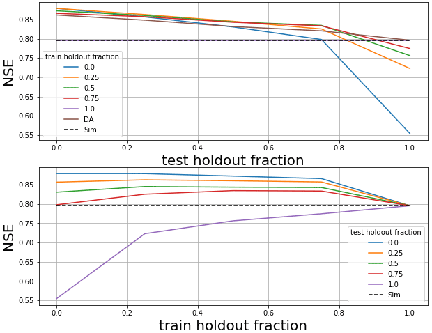
Figure 1Median NSE (Nash–Sutcliffe efficiency) scores of AR models trained and tested with different fractions of lagged streamflow data withheld. The two subplots show the same results, but organized by the amount of lagged streamflow data withheld during training vs. during testing.
2.2.2 Autoregression
The strategy that we used to deal with missing data in AR models was to replace missing lagged streamflow data with model-predicted streamflow data at the same lag time. This is related to a standard machine learning (ML) technique for training recursive models, discussed in Appendix B. Autoregression models were thus trained with two inputs in addition to the CAMELS data inputs described in Sect. 2.1: (i) streamflow lagged by some number of days (different lag times) and (ii) a binary input flag that represents whether any particular autoregressive input came from observation or from previous model predictions. The binary flag allows the model to differentiate between observed vs. simulated autoregressive inputs.

Figure 2Comparison of per-basin NSEs with an observation lag of 1 d: (a) simulation vs. DA with no missing data, (b) simulation vs. AR with no missing data, (c) AR vs. DA with no missing data, and (d) AR with no missing data vs. AR with 50 % missing data during inference (no missing data during training to be comparable with other models shown in these plots).
2.2.3 Data assimilation
The theory behind using backpropagation through tensor networks to perform variational data assimilation is given in Appendix C – this is essentially a direct implementation of standard variational DA using tensor networks.
Data assimilation was performed during the test period on the “simulation” LSTMs outlined in Sect. 2.2. Unlike training an LSTM, where all training data from all catchments must be used together to train a single model (Nearing et al., 2020; Gauch et al., 2021b), DA is independent between basins. As such, the loss function we used for data assimilation was a regularized mean squared error (MSE) (for more details on the loss function used for data assimilation, see Appendix D)

Figure 3Cumulative density function (CDF) plots of per-basin NSE scores. (a) Comparison between the main model types with no holdout. (b) Comparison of DA models with different holdout fractions during inference (testing). (c) Comparison of AR models with equal train and inference (test) holdout fractions. (d) Comparison of AR models with 50 % train holdout and varying inference holdout. All results from lead times of 1 d.
We used the ADAM optimizer for data assimilation with a dynamic learning rate that started at 0.1 and decreased by a factor of 0.9 (90 %) each time the update step loss failed to decrease. We used an assimilation window of 5 time steps (updating the cell state at time steps t−5), 100 update steps (similar to epochs) with early stopping criteria if the learning rate decreased below , and we did not use any regularization. The search used to find these hyperparameter values for data assimilation is reported in Appendix F.
2.3 Testing and evaluation
Following previous studies (cited in Sect. 2.1), we report a number of hydrologically relevant performance metrics, listed in Table 1. These metrics (and our evaluation procedure in general) were chosen to allow for benchmarking against previous studies (Kratzert et al., 2019c, b, 2021; Gauch et al., 2021a; Frame et al., 2020). Metrics in this paper are reported for now-casting, meaning that we do not use meteorological forecast data and we do not predict beyond the end of the precipitation data.
AR models were trained with fractions of missing data (withheld randomly) between 0 % and 100 %, and tested on data with different fractions of missing data. This was done to understand what effect the training data fraction has on performance. After choosing an appropriate fraction of missing data for training AR models, these models were trained with streamflow inputs that had varying lag times (between 1 and 10 d). Both AR and DA models were tested with different fractions of (randomly) withheld lagged streamflow input data and different lag times, however all metrics were calculated on all streamflow observations within each basin during the entire test period, even when some of the lagged streamflow data were withheld as inputs.

Figure 4Median NSE over 531 basins of four models (simulation, AR trained with and without holdout data, and DA) as a function of lag time in days and fraction of missing lagged streamflow data in the test period. The AR and DA models here used 0 % missing data during inference. Notice the different scales on the y axis.
Table 1Overview of evaluation metrics.
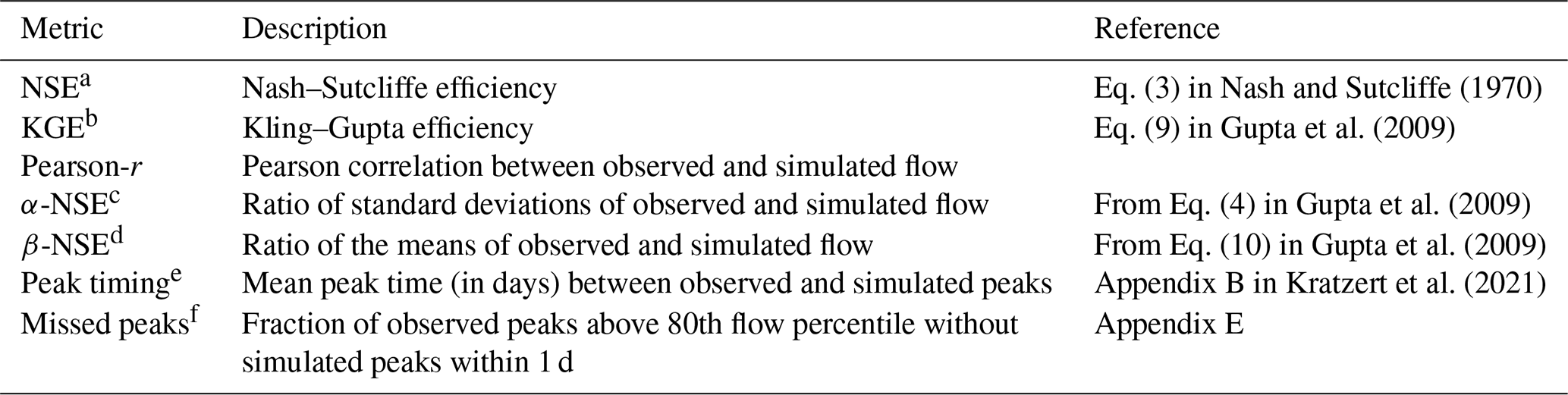
a Nash–Sutcliffe efficiency: , values closer to 1 are desirable. b Kling–Gupta efficiency: , values closer to 1 are desirable. c α-NSE decomposition: (0,∞), values close to 1 are desirable. d β-NSE decomposition: , values close to zero are desirable. e Peak-Timing: [0,∞), values close to zero are desirable. f Missed-Peaks: [0,1], values close to zero are desirable.
3.1 Training AR models with missing data
Figure 1 compares median (over test periods in 531 basins) NSE values from AR models trained with 5 missing data fractions, each tested on 5 different missing data fractions (a total of 25 inference models). The primary signal in these results is that AR models lose accuracy as the fraction of missing lagged streamflow data in the test period increases. In general, training with fewer missing data is better if the fraction of missing data in the test period is also low. However, if the fraction of missing data in the test period is high, then it is better to train with more missing data. No matter how the AR model is trained, when all lagged streamflow data are withheld during inference, performance is similar to the simulation model.
For the remainder of our experiments (including basin-split experiments), we chose to benchmark AR models trained with 50 % missing lagged streamflow inputs. This represents a compromise between training with too many or too few missing data that only degrade below the (median) accuracy of the pure simulation model with a missing data fraction of 90 %.
3.2 Time-split models
Table 2 lists the median (over 531 basins) performance metrics for all models with a lag of 1 d and no missing data. Figure 3 shows the distribution (over 531 basins) NSE scores for the same models. The major takeaways from these statistics are that both DA and AR improved over the base LSTM model but AR was better. AR (with no holdout) improved the median NSE (across test periods in 531 basins) by ∼10 %, whereas DA improved the median NSE by ∼8 %. In general, AR with no missing data performed better than DA across all metrics, and also across most basins (Fig. 2). Note that AR trained with and without any missing lagged streamflow data performed similarly with no missing data during inference.
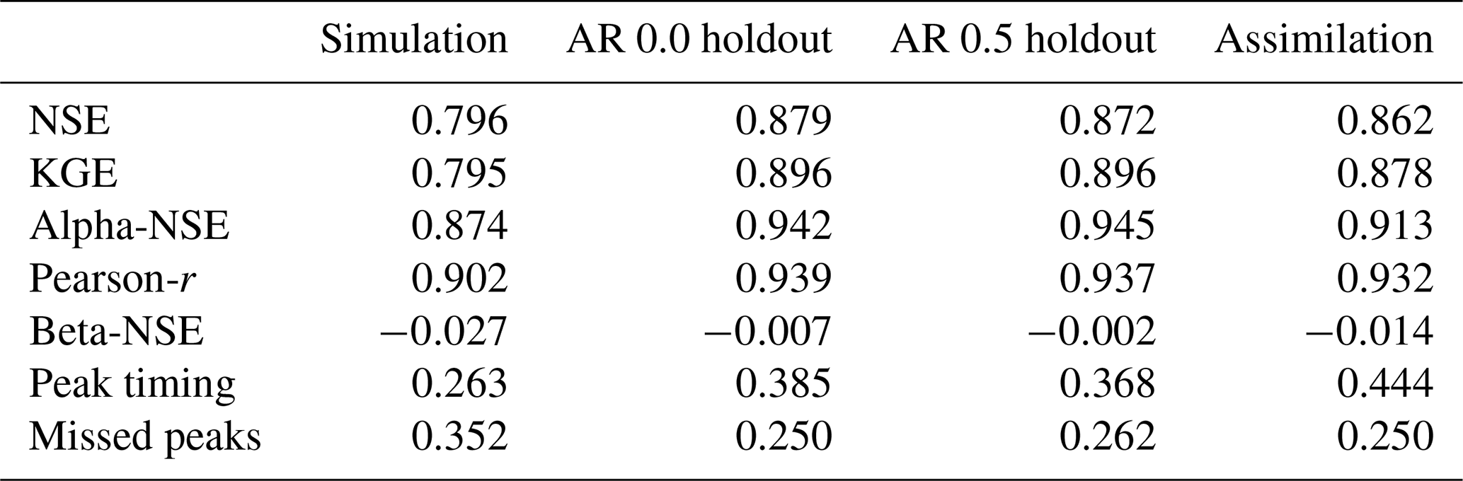
As a point of comparison with previous work, Feng et al. (2020) reported that autoregression improved LSTM median NSE by ∼19 % (from 0.714 to 0.852), whereas we saw improvement to median NSE of ∼10 % (from 0.796 to 0.879). The primary difference between that previous study and ours is that our baseline LSTMs were better (median NSE of 0.796 vs. 0.714) due to the fact that the models reported in this study used multiple forcing data products (Kratzert et al., 2021).
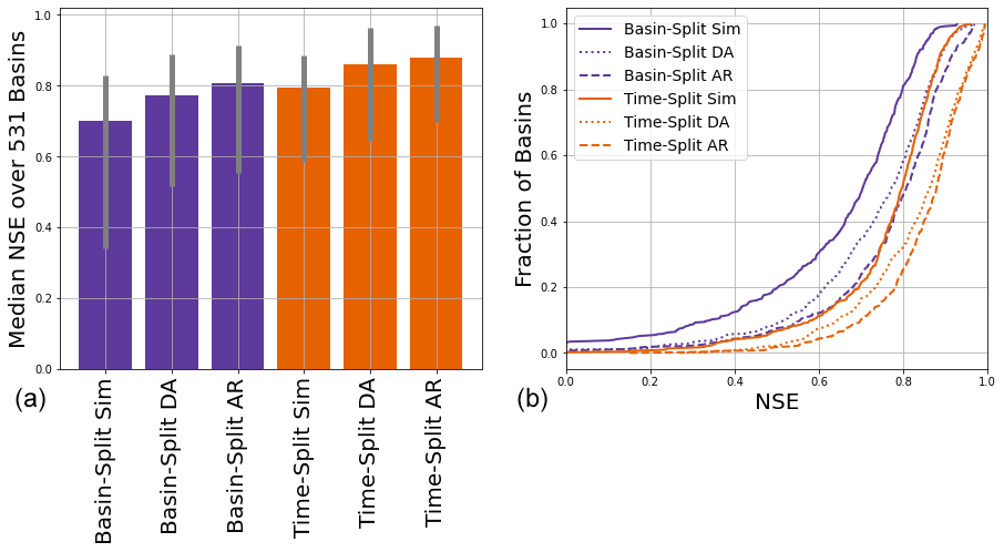
Figure 5Comparison of NSE scores between time split and basin split models at 1 d lead time with no training or inference (test) holdout. The left subplot shows median scores (over 531 basins) and 80 % interval (10th to 90th percentiles), and the right subplot shows distributions (over 531 basins).
Feng et al. (2020) also reported that autoregression was less informative in flashy basins, and there is a similar effect in our results (Appendix G reports similar efforts here to correlate differences between autoregression and data assimilation with basin attributes related to climate, geology, soils, vegetation). While both autoregression and assimilation improved the average absolute peak timing error and also allowed the model to miss fewer peak-flow events, the peak timing error with both autoregression and data assimilation was always negative due to the fact that the model receives delayed information from lagged streamflow about any peak event that it might otherwise miss predicting from meteorological data alone. That is, we predict more peaks but the ones we pick up from using real-time inputs are lagged.
Figure 4 compares the median NSE scores (over 531 basins) between the four models as a function of lag time in days and fraction of missing lagged streamflow data in the test period. AR is always better than DA, but if the DA model is not trained with a fraction of missing data (here 50 %), then performance decreases whenever there is missing data in the test period. In this case, the autoregression model can perform worse than a simulation model with no lagged streamflow data. If the autoregression model is trained with an input flag to indicate whether a particular lagged streamflow value is from observation or simulation, then autoregression almost always improves on the baseline simulation model and is almost always better than data assimilation (up to large values of missing data). Similar figures for all metrics in Table 1 are given in Appendix H.
3.3 Basin-split models
Figure 5 compares the time-split and basin-split results at 1 d lead time with no training or test holdout. Previous studies have shown that LSTM models can often be used to predict in basins that did not supply training data, and the purpose of these basin-split experiments was to assess whether this ability to generalize holds when using observation data as inputs. This covers a class of use cases where data are not available for training in a given basin, but become available during inference, but more importantly, it helps us assess whether the model is learning general relationships between past and future streamflow.
Results in Fig. 5 show that this is the case. The main thing to highlight in these results is that AR in basins that were “ungauged” for training but where data were available during inference (the basin-split AR model) generally performed better than basins where data were available for training but not for inference (the time-split simulation model). This indicates that adding AR to the model does not break extrapolatability – for example, the model learns a general representation of relationships between past streamflow and current inputs, and can extrapolate those relationships to new basins. It does not simply learn to extrapolate streamflow in basins where it was trained.
Data assimilation is necessary in order to use certain types of data to “drive” dynamical systems models. For example, if a model is based on some conceptual understanding of a physical system (like a conceptual process-based rainfall–runoff model), then the only way to use observations of system states or outputs is through some type of inverse method. DA is a class of inverse methods that project information onto the states of a dynamical systems model. DA is often complicated to set up (e.g., choosing parameters to represent uncertainty distributions, sampling procedures), and often requires simplifying assumptions that cause significant information loss (e.g., Nearing et al., 2018, 2013). ML models do not necessarily suffer from these same limitations – it is possible to simply train models to use whatever data are available. This has several advantages, including ease of use (no additional hyperparameter tuning), computational efficiency (see below), and apparently from our results, an increase in accuracy (less information loss).
It is worth noting that in the experiments presented here, running DA for inference on the 10 yr test period in 531 basins required approximately ∼2 h of GPU time (NVIDIA Tesla v100) using the hyperparameters specified in Appendix F. Inference over the same basins and time period with an AR model required ∼30 min, and simulation required less than 5 min. The reason that AR is more expensive than simulation is because the AR LSTM is not CUDA-optimized, since the tensor network includes a gradient path from outputs to inputs. It might be possible to design an optimized version of this model (similar to the PyTorch-optimized LSTM), however this is significantly outside the scope of our project.
DA has one advantage: it does not require that we choose how to withhold inputs to train the model. In cases where there are no target data during inference, AR models have potential to perform worse than a simulation model (see Fig. 3), whereas DA models do not. DA reverts to a pure simulation model when there are no data to assimilate. This means that if the purpose of a model were to predict in a combination of gauged and ungauged basins, DA would allow you to use one trained model whereas AR would require separate models for gauged and ungauged basins. In principle, you would likely choose whether to use a simulation model or an AR model dynamically based on whether streamflow data were available at the time and place of each individual prediction.
To reiterate from the introduction, both DA and AR are broad classes of methods. We do not know of any benchmarking study in the hydrology literature that directly compares different DA methods over large, standardized, public data sets. Most DA methods are based on some type of inverse algorithm, which cause information loss e.g., Nearing et al. (2018). Whereas inverse methods require making strong assumptions about the characteristics of model and data error, generative models, like the LSTM models used here, do not. To summarize, our conclusion is that it is cheaper, easier, and generally more accurate to simply give your models all the data you have as inputs whenever possible.
Streamflow input data were sampled at different missing data fractions for training and testing AR models and for DA. We masked continuous periods of missing data by using two Bernoulli samplers. We sampled “downshifts” and “upshifts” through a time series at different rates (ρd and ρu, respectively). Moving sequentially through a time series, downshifts indicate that the missing data mask is turned on (a period of missing data begins), and upshifts indicate that the missing data mask turns off (a period of missing data ends). The ρd and ρu were chosen as to yield a mask with two properties: (i) an average masking sequence length of a given length (we used 5 time steps), and (ii) a total masking density of a given percentage of the whole time series. These relationships are
The strategy we use for handling missing data in AR models is loosely related to a class of techniques used commonly to train recursive neural networks called teacher-forcing methods (Williams and Zipser, 1989). Teacher-forcing methods substitute model outputs from time step t as inputs into the network at time step t+1 with observations during training (not during inference). This was originally used to avoid backpropagating through time, and the method is sensitive to differences between train and test samples which can result in divergent behavior when the model is run recursively during inference.
Our strategy for dealing with missing data in AR models does not replace the cell state (the recursive state of the LSTM) during training, but does run the risk of over-training to observed lagged streamflow inputs in cases where these data are sparse during inference (Fig. 1). Our solution to this problem is to train with a combination of observed and simulated lagged streamflow inputs, which is a form of scheduled sampling (Bengio et al., 2015). This seems to work in this case (see Sect. 3.1). Another class of approaches to solving this problem are professor-forcing methods (Lamb et al., 2016), which uses adversarial learning to encourage a teacher-forcing network (i.e., trained with only observed inputs) to match the fully recursive model. This could be applied to the streamflow problem if AR models were to exhibit divergent behavior that cannot be solved with scheduled sampling.
The method of data assimilation that we will use in this paper is a type of variational assimilation. Variational assimilation works as follows (Rabier and Liu, 2003). We begin with a model that has time-dependent states, c[t], that determine a time-dependent observable, y[t], through a (potentially nonlinear) observation operator, ℋ, up to random error, εy[t]:
The model itself propagates through time according to some state transition function, ℳ, that operates on the state at the previous time step and model inputs, x[t]:
The background state, cb[t], is the state estimated by model ℳ at time t without performing assimilation at time t (although assimilation may have been performed at previous time steps). The true (but unknown) state of the system is assumed to be equal to the background state up to random error εc:
Notating observations and states as drawn from distributions py and pc, we condition the model state on observations at time t as
The maximum likelihood estimate of the state vector is found by minimizing the negative log likelihood associated with Eq. (C4). For example, if the state and observation errors (εc and εy) are assumed to be normally distributed, the resulting loss function is
where B and R are covariances of the state and observation errors, respectively. Analytical solutions are known for the special case when ℋ(⋅) is linear. Equation (C5) can be understood as a regularized loss function acting on target variables that is to be maximized with respect to the model states. If any component of this is not linear and Gaussian, then 𝒥(⋅) must be minimized numerically.
The LSTM is described by the following equations:
x[t] are again the model inputs at time t, and i[t], f[t], and o[t] refer to the input gate, forget gate, and output gate of the LSTM, respectively. g[t] are the cell inputs, h[t−1] are the LSTM outputs, which are also called the recurrent input because these are used as inputs to all gates in the next time step. c[t−1] is the cell state from the previous time step. Similar to dynamical systems models, the cell state, c[t], tracks the time evolution of the system.
Model-predicted streamflow values comes from a head layer, and many LSTM studies in hydrology (e.g., Kratzert et al., 2018) have used a linear (dense) head layer:
Equations (C11) and (C12) effectively define the observation operator for data assimilation (Eq. C1). Notice that observations y[t] are not linear functions of the cell state (through the hyperbolic tangent operator in Eq. C11), so no analytical solution to maximizing Eq. (C4) or minimizing Eq. (C5) exists. We therefore must minimize 𝒥(c[t]) numerically, which requires gradients with respect to the cell states.
In any deep learning model, the various weights, W*, and biases, b*, are trained by minimizing a training loss function, L(⋅), using backpropagation along gradient chains like
where the subscripts j and k (e.g., , hk[t]) indicate arbitrary components of vectors or matrices (e.g., W* like Wi, Wf, Wo, or Wg). h[t−1] are again the LSTM outputs (recurrent inputs), and the ellipses indicate that the network may have arbitrary depth. Equation (C13) is a simple derivative chain rule that any machine learning software library calculates automatically through the entirety of whatever tensor network defines a particular model. Almost all deep learning models are trained by backpropagating information through this type of gradient chain. Every time that the training loss function L(⋅) is calculated on a series of model inputs, x[0:t], and outputs, y[0:t], the values of all weights and biases in the model are updated based on perturbing in a direction that will decrease the loss according to these partial derivatives.
Notice that gradient chains like Eq. (C13) necessarily include partial derivatives of the loss function with respect to features in the model that are not weights and biases. As an example, the partial derivative of loss L with respect to weights in the input gate, Wi, requires derivatives with respect to the cell states, c[t]. To perform data assimilation, we can simply break the gradient chains to get partial derivatives of a loss function with respect to cell states like
Gradient chains like Eq. (C13) are used when training deep learning models. In this case, the loss function is calculated over a large number of historical data points (sometimes using minibatches). We want to be able to use streamflow observation data as they become available in near-real-time, which means that we want to use gradient chains like Eq. (C14) during inference rather than during training. These take the following form:
The primary difference between Eqs. (C14) and (C15) is that the loss function is calculated over observations within a finite time period, s, into the past, , and used to update cell states at the start of that observation period. We call s the assimilation window. After the model is fully trained, and while it is running in forward mode to make new predictions, we can at any point calculate a loss function like , and use this to update the cell states of the LSTM using gradient chains like Eq. (C15).
The loss functions used for assimilation (i.e., ℒ(⋅) in Eq. C15) do not need to be the same loss functions used for training (i.e., L in Eq. C13). The derivatives that result from gradient chains in a deep learning tensor network can be calculated with respect to any loss function. Additionally, any loss function can be augmented with regularization – for example, to ensure that the updated cell states do not deviate too much from the values that are estimated by the trained model. The R and B matrices in Eq. (C5) are an example of this type of regularization, and it is trivial to use this (or any other) type or regularization in the data assimilation loss function.
Coefficients αc and αy are constants that are analogous to the B and R terms in Eq. (C5). Since in this form these are mixing parameters, our experiments assume that . The assimilation window, s, is as in Eq. (C15). Gradient chains like Eq. (C15) do not look forward in time in the sense that the derivative of ℒ with respect to c[t] does not depend on any observation prior to time t. This means that the assimilation loss Eq. (D1) is general in s.
The missed peaks metric is calculated by first locating all peaks in the observation and simulation time series that satisfy the following two criteria: (1) observed and simulated peaks must be at least 30 d apart, and (2) peaks must be above the 80th flow percentile in a given basin. Any peak in the observed time series that meets these two criteria and for which there is not a peak in the simulated time series that also meets these criteria within 1 d (before or after) is considered a missed peak. We report the fraction of observed peaks that are missed.
Hyperparameter tuning for data assimilation was done with a validation period (1980–1989) that is distinct from both the training (1999–2008) and test periods (1989–1999) outlined in Sect. 2.2.1. Due to computational expense, hyperparameter tuning was done on a subset of 53 basins out of the 531 used for the rest of the study (approximately 10 %). We used a simple grid search, which is outlined in Table F1. This grid search resulted in the final data assimilation hyperparameters listed in the right-most column of Table F1.
Table F1Data assimilation hyperparameter tuning grid search and final values.
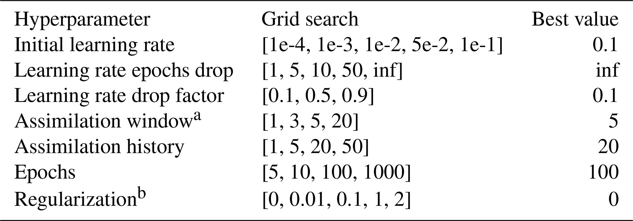
We used a learning rate scheduler that dropped the learning rate every N epochs. This is the learning rate epochs drop hyperparameter in Table F1 and did not improve performance. Because we used sequence-to-one prediction, we did not perform assimilation through the entire time series, and the assimilation history hyperparameter determines how far back in each sequence (before time of prediction) we start assimilation. This parameter is a multiple of the assimilation window. The assimilation window itself is s in Eq. (C15).
In our setup, αc (see Eq. D1) was set as a hyperparameter and not trained directly, although learning this parameter through backpropagation is possible. Our hyperparameter search returned a value of αc=0 (and implied value of αy=1), meaning that regularizing the loss function was not helpful.
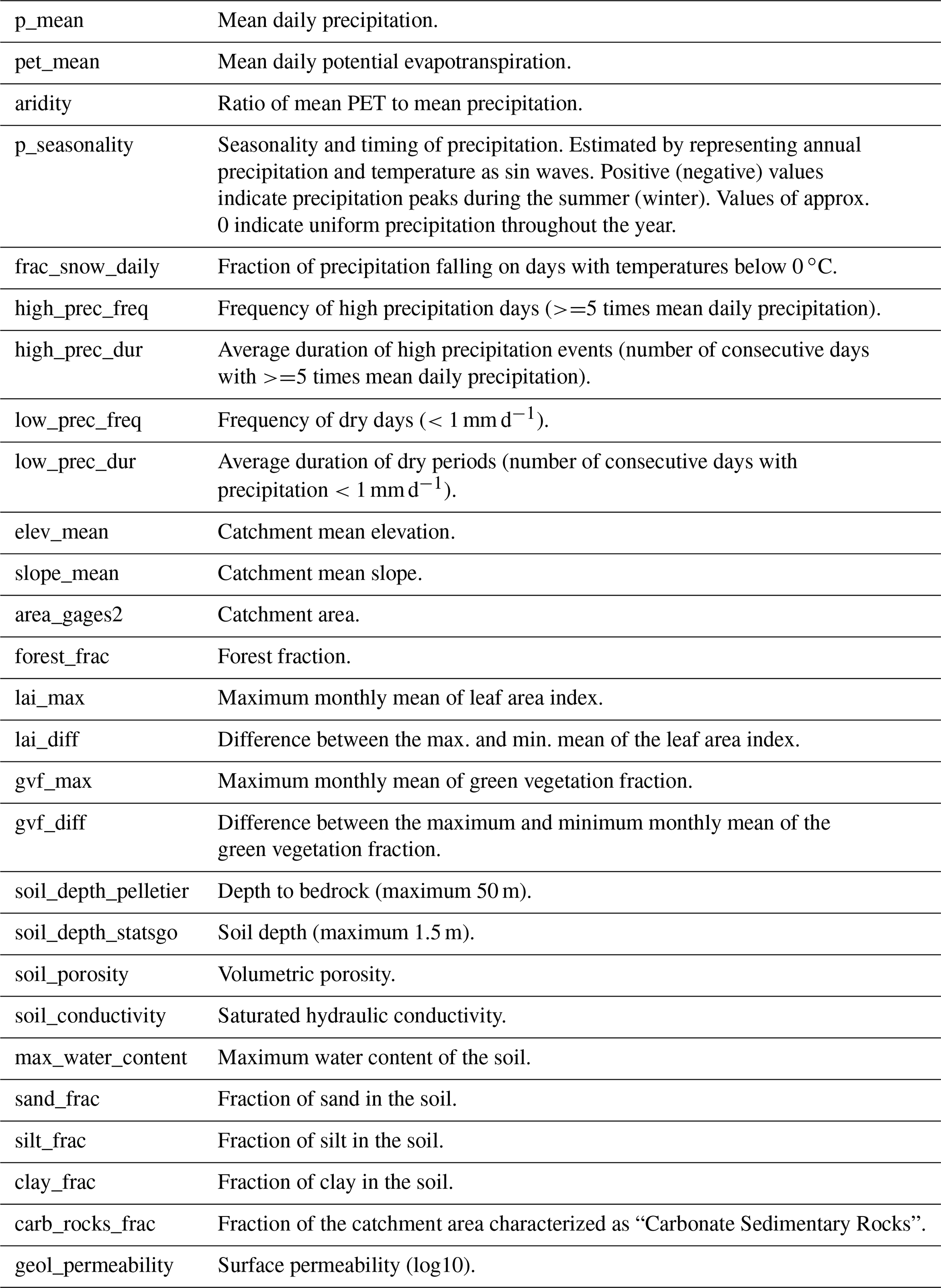
We tested whether it was possible to predict where DA or AR might offer the most benefit by using CAMELS catchment attributes (Addor et al., 2017). These attributes and their abbreviations are listed in Table G1. We used random forest models trained with static catchment attributes as inputs using k-fold cross validation to measure the predictability of the increase or decrease in test-period NSE scores at individual basins. The objective was to determine which types of hydrological characteristics determine the value or information content of lagged streamflow data.
Table G1Table of static catchment attributes. Descriptions taken from Addor et al. (2017).
Results for this analysis are given in Fig. G1. The top subplots of Fig. G1 illustrate the ability to predict test-period NSE scores from basin attributes in the three models (simulation, AR, DA), and the bottom subplots illustrate the ability to predict differences between test-period NSE scores from the different models. Kratzert et al. (2019c) found that forest fraction was strongly correlated with a predictor of the basin similarity mapping in an LSTM, and we see a similar effect in the top left subplot of Fig. G1 (forest fraction is the second-highest predictor of the skill of the simulation model).
Feng et al. (2020) reported that AR was less informative in flashy basins, and we see some evidence of that effect here: in particular, the frequency of low precipitation days was the strongest predictor of AR skill such that lower fractions of rainfall occurring in low intensity events corresponds with higher AR skill. Similarly, basin area was the third-strongest predictor of AR skill, with AR being better in larger basins.
Snow fraction was the second strongest predictor of skill for both AR and DA, whereas this was not a strong predictor of skill in the pure simulation model. Kratzert et al. (2019a) showed that LSTMs can learn to store and release snow (without seeing snow data), however snowpack introduces correlations in streamflow time series that are exploited by both DA and AR.
The basin attributes that were the most important for determining NSE improvements due to both DA and AR (bottom center and bottom right subplots of Fig. G1) were (i) mean annual precipitation and (ii) high precipitation frequency. High precipitation frequency was positively correlated with both AR and DA performance improvements. The reason for this is error in the rainfall data – AR and DA allow the model to effectively “see” streamflow events that occur due to unobserved or under-observed rainfall, although it takes 1 time step for the model to register that a large event happened. This helps the model to avoid large errors for events with long recession curves. In general, average precipitation was negatively correlated with improvements due to incorporating lagged streamflow data, since precipitation events in general reduce autocorrelation in the streamflow time series. This effect appears worse for DA than AR (bottom left subplot), although this is a weak signal because we were generally unable to predict differences between the NSE scores of DA and AR (r2=0.12; bottom right subplot in Fig. G1).
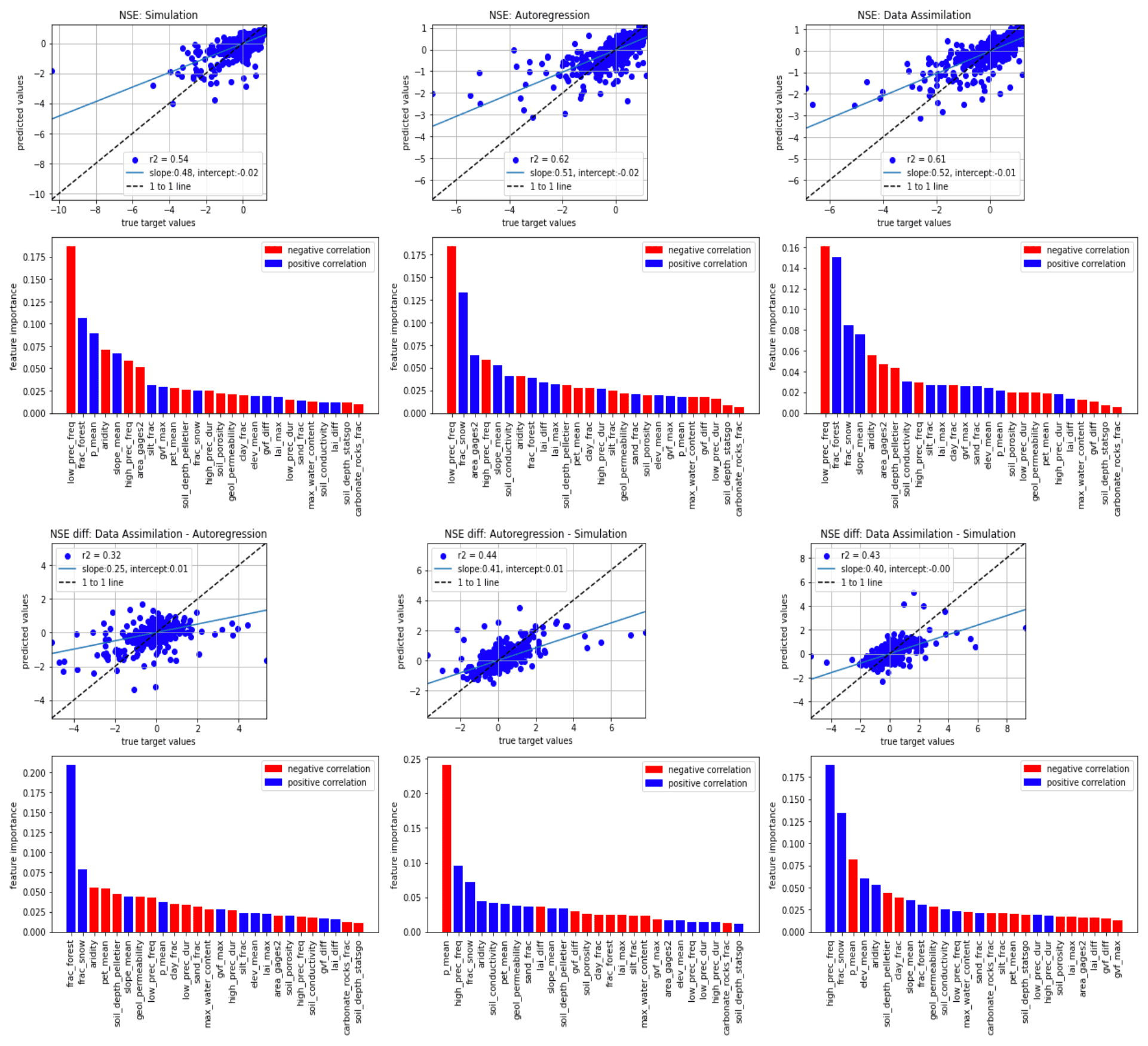
Figure G1Scatterplots, r2 metrics, and feature importances for predicting test-period NSE scores using different models (top subplots), and for predicting differences between models (bottom subplots). Bar charts show the feature importance for these predictions with blue indicating positive correlations between a given basin attribute and the NSE (or delta-NSE) and red indicating a negative correlation.
Figure G2 shows the spatial distribution of DA and AR NSE improvements relative to simulation. In both cases – but especially for DA – there is a group of basins in the Midwest and southeast United States where performance was harmed by adding lagged streamflow data. We are unsure of the reason for this, but it warrants further exploration.

Figure G2The performance difference (NSE score) between top: autoregression and the baseline simulation, and bottom: data assimilation and the baseline simulation.
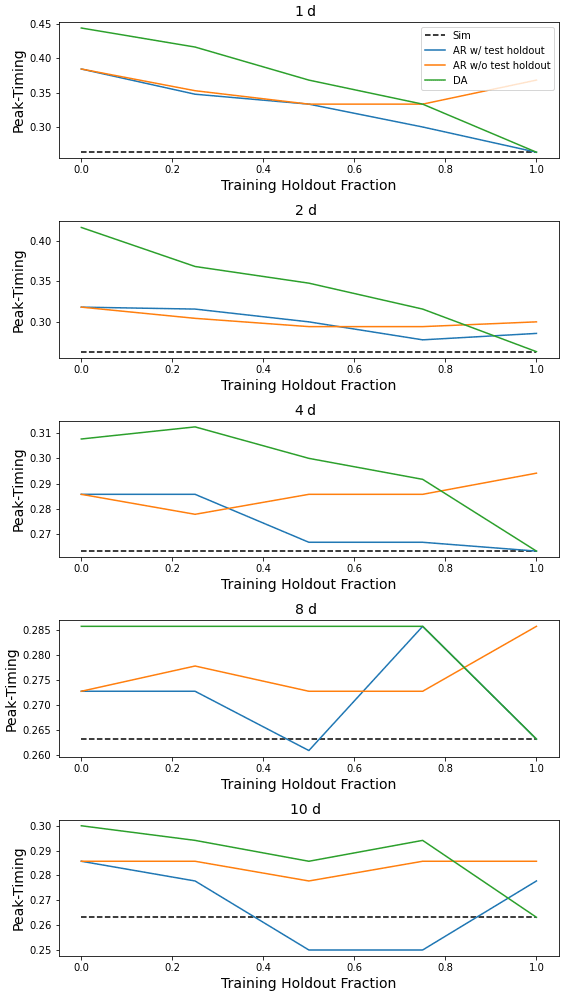
This appendix contains figures similar to Fig. 4 for all metrics listed in Table 1. These figures compare the median (over 531 basins) performance of four models (simulation, autoregression trained with and without holdout data, and data assimilation) as a function of lag time in days and fraction of missing lagged streamflow data in the test period.
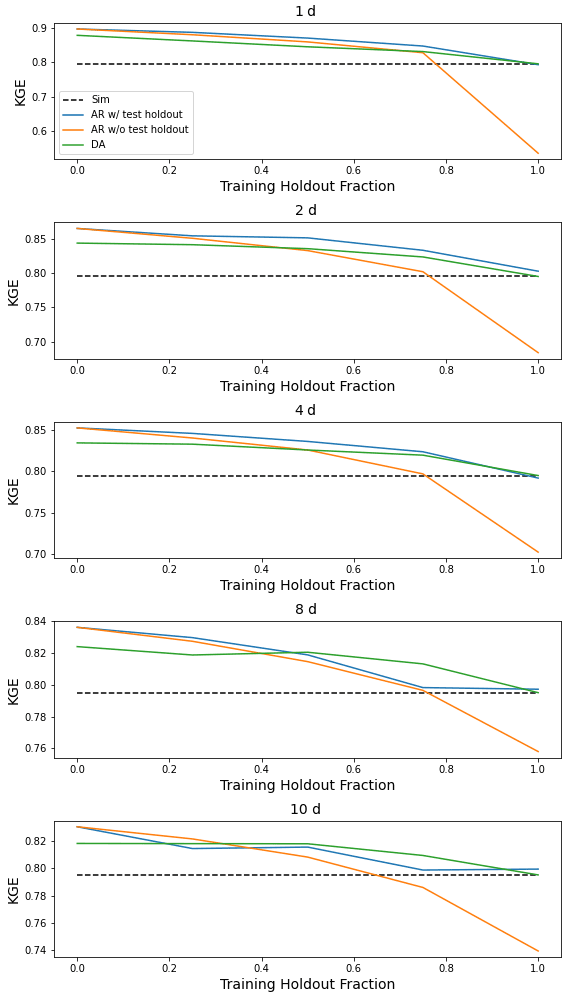
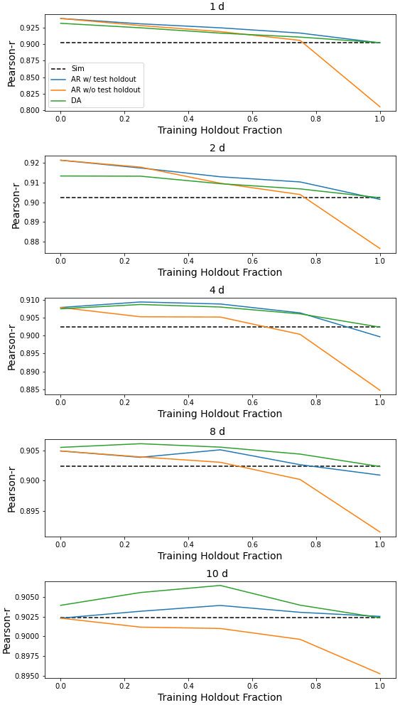
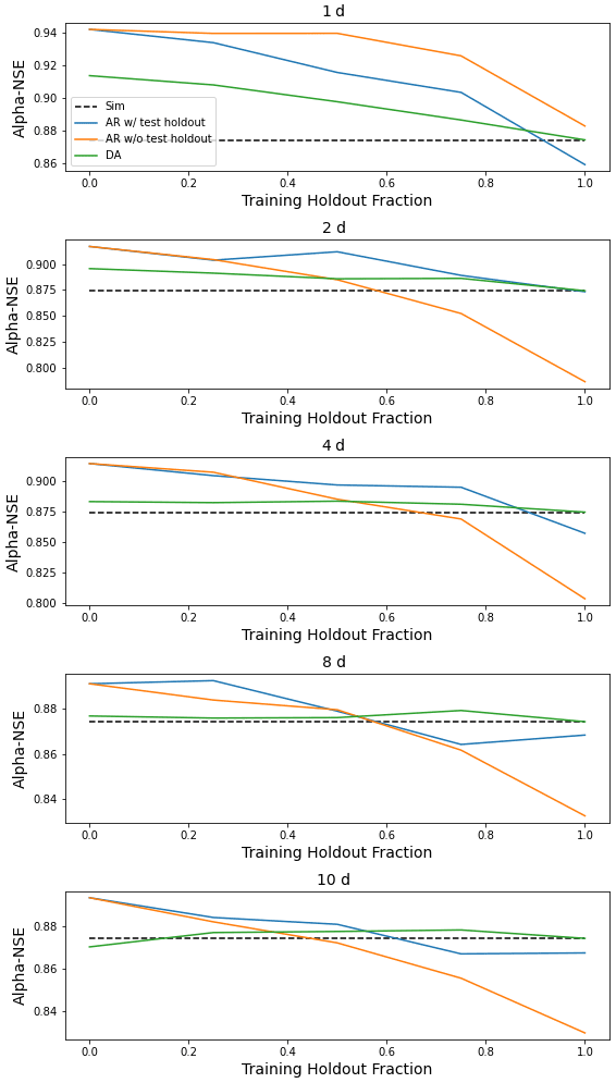
Figure H3Same as Fig. 4 but for α-NSE, which is the ratio of the standard deviation of the observed vs. modeled hydrographs.
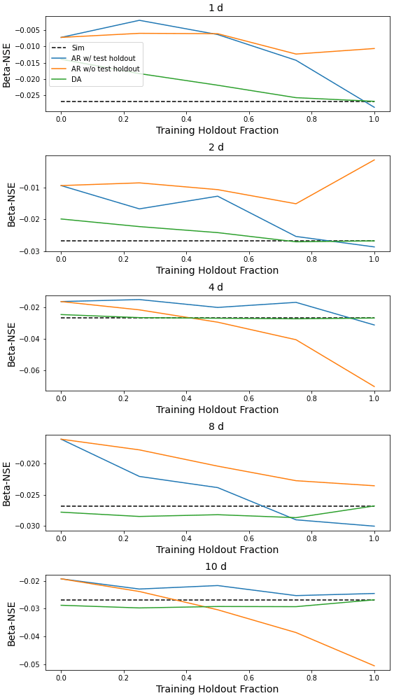
Figure H4Same as Fig. 4 but for β-NSE, which is the ratio of the means of the observed vs. modeled hydrographs.

Plug-and-play code to reproduce the experiments reported in this paper is available at https://doi.org/10.5281/zenodo.7063252 (Kratzert et al., 2022a). Model code, including data assimilation and autoregression, is available at https://doi.org/10.5281/zenodo.7063259 (Kratzert et al., 2022b). This is a fork of the NeuralHydrology codebase (https://neuralhydrology.github.io/). The fork contains a branch called “assimilation” that contains code necessary for data assimilation. CAMELS data are available at https://doi.org/10.5065/D6MW2F4D (Newman et al., 2014), with extensions to 2014 at https://doi.org/10.4211/hs.0a68bfd7ddf642a8be9041d60f40868c (Kratzert, 2019a) and https://doi.org/10.4211/hs.17c896843cf94033 (Kratzert, 2019b).
DK, AKS, and GSN had the original idea for backpropagation-based data assimilation. All authors contributed to experimental design. GSN wrote the data assimilation code, performed hyperparameter tuning, and conducted all experiments except correlations with basin attributes, which were done by JMF. All authors contributed to experimental design. MG suggested to implement the input data flag for autoregression (which was transformative for AR skill). GSN, MG, DK, and FK integrated the data assimilation code into the NeuralHydrology codebase. GSN wrote the paper with contributions from all authors.
The contact author has declared that none of the authors has any competing interests.
Publisher’s note: Copernicus Publications remains neutral with regard to jurisdictional claims in published maps and institutional affiliations.
Frederik Kratzert was supported by a Google Faculty Research Award (PI: Sepp Hochreiter). Martin Gauch was supported by the Linz Institute of Technology DeepFlood project. Daniel Klotz was supported by Verbund AG.
This paper was edited by Erwin Zehe and reviewed by Ralf Loritz and one anonymous referee.
Abrahart, R. J. and See, L.: Comparing neural network and autoregressive moving average techniques for the provision of continuous river flow forecasts in two contrasting catchments, Hydrol. Proc., 14, 2157–2172, 2000. a
Addor, N., Newman, A. J., Mizukami, N., and Clark, M. P.: The CAMELS data set: catchment attributes and meteorology for large-sample studies, Hydrol. Earth Syst. Sci., 21, 5293–5313, https://doi.org/10.5194/hess-21-5293-2017, 2017. a, b, c, d
Bannister, R.: A review of operational methods of variational and ensemble-variational data assimilation, Q. J. Roy. Meteor. Soc., 143, 607–633, 2017. a
Bengio, S., Vinyals, O., Jaitly, N., and Shazeer, N.: Scheduled sampling for sequence prediction with recurrent neural networks, arXiv [preprint], https://doi.org/10.48550/arXiv.1506.03099, 2015. a
Cameron, D., Kneale, P., and See, L.: An evaluation of a traditional and a neural net modelling approach to flood forecasting for an upland catchment, Hydrol. Proc., 16, 1033–1046, https://doi.org/10.1002/hyp.317, 2002. a
Child, R.: Very deep vaes generalize autoregressive models and can outperform them on images, arXiv [preprint], https://doi.org/10.48550/arXiv.2011.10650, 2020. a
Chollet, F.: Deep learning with Python, Simon and Schuster, ISBN-13: 9781617296864, 2017. a
De Fauw, J., Dieleman, S., and Simonyan, K.: Hierarchical autoregressive image models with auxiliary decoders, arXiv [preprint], https://doi.org/10.48550/arXiv.1903.04933, 2019. a
Del Moral, P.: Nonlinear filtering: Interacting particle resolution, Comptes Rendus de l'Académie des Sciences-Series I-Mathematics, 325, 653–658, 1997. a
Dhariwal, P., Jun, H., Payne, C., Kim, J. W., Radford, A., and Sutskever, I.: Jukebox: A generative model for music, arXiv [preprint], https://doi.org/10.48550/arXiv.2005.00341, 2020. a
Dong, W., Fong, D. Y. T., Yoon, J.-s., Wan, E. Y. F., Bedford, L. E., Tang, E. H. M., and Lam, C. L. K.: Generative adversarial networks for imputing missing data for big data clinical research, BMC Med. Res. Methodol., 21, 1–10, 2021. a
Dosovitskiy, A. and Brox, T.: Inverting visual representations with convolutional networks, in: Proceedings of the IEEE conference on computer vision and pattern recognition, 4829–4837, 2016. a
Evensen, G.: The ensemble Kalman filter: Theoretical formulation and practical implementation, Ocean Dynam., 53, 343–367, 2003. a
Feng, D., Fang, K., and Shen, C.: Enhancing streamflow forecast and extracting insights using long-short term memory networks with data integration at continental scales, Water Resour. Res., 56, e2019WR026793, 2020. a, b, c, d
Fernandez, B. and Salas, J. D.: Periodic gamma autoregressive processes for operational hydrology, Water Resour. Res., 22, 1385–1396, 1986. a
Frame, J., Nearing, G., Kratzert, F., and Rahman, M.: Post processing the US national water model with a long short-term memory network, J. Am. Water Resour. As., https://doi.org/10.31223/osf. io/4xhac, 2020. a
Frame, J. M., Kratzert, F., Klotz, D., Gauch, M., Shalev, G., Gilon, O., Qualls, L. M., Gupta, H. V., and Nearing, G. S.: Deep learning rainfall–runoff predictions of extreme events, Hydrol. Earth Syst. Sci., 26, 3377–3392, https://doi.org/10.5194/hess-26-3377-2022, 2022. a, b, c
Gauch, M., Kratzert, F., Klotz, D., Nearing, G., Lin, J., and Hochreiter, S.: Rainfall–runoff prediction at multiple timescales with a single Long Short-Term Memory network, Hydrol. Earth Syst. Sci., 25, 2045–2062, https://doi.org/10.5194/hess-25-2045-2021, 2021a. a, b
Gauch, M., Mai, J., and Lin, J.: The proper care and feeding of CAMELS: How limited training data affects streamflow prediction, Environ. Modell. Softw., 135, 104926, 2021b. a, b
Gaume, E. and Gosset, R.: Over-parameterisation, a major obstacle to the use of artificial neural networks in hydrology?, Hydrol. Earth Syst. Sci., 7, 693–706, https://doi.org/10.5194/hess-7-693-2003, 2003. a
Gers, F. A., Schmidhuber, J., and Cummins, F.: Learning to forget: Continual prediction with LSTM, Neural Comput., 12, 2451–2471, 2000. a
Graves, A.: Generating sequences with recurrent neural networks, arXiv [preprint], https://doi.org/10.48550/arXiv.1308.0850, 2013. a
Gregor, K., Danihelka, I., Graves, A., Rezende, D., and Wierstra, D.: Draw: A recurrent neural network for image generation, in: International Conference on Machine Learning, 1462–1471, 2015. a
Gupta, H. V., Kling, H., Yilmaz, K. K., and Martinez, G. F.: Decomposition of the mean squared error and NSE performance criteria: Implications for improving hydrological modelling, J. Hydrol., 377, 80–91, 2009. a, b, c
Hsu, K.-L., Gupta, H. V., and Sorooshian, S.: Artificial neural network modeling of the rainfall-runoff process, Water Resour. Res., 31, 2517–2530, 1995. a
Kim, J., Tae, D., and Seok, J.: A survey of missing data imputation using generative adversarial networks, in: 2020 International Conference on Artificial Intelligence in Information and Communication (ICAIIC), IEEE, 454–456, 2020. a
Klotz, D., Kratzert, F., Gauch, M., Keefe Sampson, A., Brandstetter, J., Klambauer, G., Hochreiter, S., and Nearing, G.: Uncertainty estimation with deep learning for rainfall–runoff modeling, Hydrol. Earth Syst. Sci., 26, 1673–1693, https://doi.org/10.5194/hess-26-1673-2022, 2022. a
Kratzert, F.: CAMELS Extended NLDAS Forcing Data, HydroShare [data set], https://doi.org/10.4211/hs.0a68bfd7ddf642a8be9041d60f40868c, 2019a. a
Kratzert, F.: CAMELS Extended Maurer Forcing Data, HydroShare [data set], https://doi.org/10.4211/hs.17c896843cf940339c3c3496d0c1c077, 2019b. a
Kratzert, F., Klotz, D., Brenner, C., Schulz, K., and Herrnegger, M.: Rainfall–runoff modelling using Long Short-Term Memory (LSTM) networks, Hydrol. Earth Syst. Sci., 22, 6005–6022, https://doi.org/10.5194/hess-22-6005-2018, 2018. a
Kratzert, F., Herrnegger, M., Klotz, D., Hochreiter, S., and Klambauer, G.: Neuralhydrology–interpreting lstms in hydrology, in: Explainable ai: Interpreting, explaining and visualizing deep learning, Springer, 347–362, 2019a. a
Kratzert, F., Klotz, D., Herrnegger, M., Sampson, A. K., Hochreiter, S., and Nearing, G. S.: Toward Improved Predictions in Ungauged Basins: Exploiting the Power of Machine Learning, Water Resour. Res., 55, 11344–11354, https://doi.org/10.1029/2019WR026065, 2019b. a, b, c
Kratzert, F., Klotz, D., Shalev, G., Klambauer, G., Hochreiter, S., and Nearing, G.: Towards learning universal, regional, and local hydrological behaviors via machine learning applied to large-sample datasets, Hydrol. Earth Syst. Sci., 23, 5089–5110, https://doi.org/10.5194/hess-23-5089-2019, 2019c. a, b, c, d, e, f, g
Kratzert, F., Gauch, M., Nearing, G., and Klotz, D.: NeuralHydrology – A Python library for Deep Learning research in hydrology, Zenodo [code] https://doi.org/10.5281/zenodo.7063252, 2022a. a
Kratzert, F., Gauch, M., Nearing, G., and Klotz, D.: NeuralHydrology – A Python library for Deep Learning research in hydrology (v.1.3.0), Zenodo [code], https://doi.org/10.5281/zenodo.7063259, 2022b. a
Kratzert, F., Klotz, D., Hochreiter, S., and Nearing, G. S.: A note on leveraging synergy in multiple meteorological data sets with deep learning for rainfall–runoff modeling, Hydrol. Earth Syst. Sci., 25, 2685–2703, https://doi.org/10.5194/hess-25-2685-2021, 2021. a, b, c, d, e
Lamb, A. M., Goyal, A. G. A. P., Zhang, Y., Zhang, S., Courville, A. C., and Bengio, Y.: Professor forcing: A new algorithm for training recurrent networks, in: Advances in neural information processing systems, 4601–4609, 2016. a
Mahendran, A. and Vedaldi, A.: Understanding deep image representations by inverting them, in: Proceedings of the IEEE conference on computer vision and pattern recognition, 5188–5196, 2015. a
Mai, J., Shen, H., Tolson, B. A., Gaborit, É., Arsenault, R., Craig, J. R., Fortin, V., Fry, L. M., Gauch, M., Klotz, D., Kratzert, F., O'Brien, N., Princz, D. G., Rasiya Koya, S., Roy, T., Seglenieks, F., Shrestha, N. K., Temgoua, A. G. T., Vionnet, V., and Waddell, J. W.: The Great Lakes Runoff Intercomparison Project Phase 4: the Great Lakes (GRIP-GL), Hydrol. Earth Syst. Sci., 26, 3537–3572, https://doi.org/10.5194/hess-26-3537-2022, 2022. a, b
Matalas, N. C.: Mathematical assessment of synthetic hydrology, Water Resour. Res., 3, 937–945, 1967. a
Moshe, Z., Metzger, A., Elidan, G., Kratzert, F., Nevo, S., and El-Yaniv, R.: Hydronets: Leveraging river structure for hydrologic modeling, arXiv [preprint], https://doi.org/10.48550/arXiv.2007.00595, 2020. a
Nash, J. E. and Sutcliffe, J. V.: River flow forecasting through conceptual models part I – A discussion of principles, J. Hydrol., 10, 282–290, 1970. a
Nearing, G., Yatheendradas, S., Crow, W., Zhan, X., Liu, J., and Chen, F.: The efficiency of data assimilation, Water Resour. Res., 54, 6374–6392, 2018. a, b, c
Nearing, G. S., Gupta, H. V., and Crow, W. T.: Information loss in approximately Bayesian estimation techniques: A comparison of generative and discriminative approaches to estimating agricultural productivity, J. Hydrol., 507, 163–173, 2013. a
Nearing, G. S., Kratzert, F., Sampson, A. K., Pelissier, C. S., Klotz, D., Frame, J. M., Prieto, C., and Gupta, H. V.: What role does hydrological science play in the age of machine learning?, Water Resour. Res., 57, e2020WR028091, https://doi.org/10.1029/2020WR028091, 2020. a
Nevo, S., Morin, E., Gerzi Rosenthal, A., Metzger, A., Barshai, C., Weitzner, D., Voloshin, D., Kratzert, F., Elidan, G., Dror, G., Begelman, G., Nearing, G., Shalev, G., Noga, H., Shavitt, I., Yuklea, L., Royz, M., Giladi, N., Peled Levi, N., Reich, O., Gilon, O., Maor, R., Timnat, S., Shechter, T., Anisimov, V., Gigi, Y., Levin, Y., Moshe, Z., Ben-Haim, Z., Hassidim, A., and Matias, Y.: Flood forecasting with machine learning models in an operational framework, Hydrol. Earth Syst. Sci., 26, 4013–4032, https://doi.org/10.5194/hess-26-4013-2022, 2022. a
Newman, A., Sampson, K., Clark, M. P., Bock, A., Viger, R. J., and Blodgett, D.: A large-sample watershed-scale hydrometeorological dataset for the contiguous USA, UCAR/NCAR [data set], https://doi.org/10.5065/D6MW2F4D, 2014. a
Newman, A. J., Clark, M. P., Sampson, K., Wood, A., Hay, L. E., Bock, A., Viger, R. J., Blodgett, D., Brekke, L., Arnold, J. R., Hopson, T., and Duan, Q.: Development of a large-sample watershed-scale hydrometeorological data set for the contiguous USA: data set characteristics and assessment of regional variability in hydrologic model performance, Hydrol. Earth Syst. Sci., 19, 209–223, https://doi.org/10.5194/hess-19-209-2015, 2015. a
Newman, A. J., Mizukami, N., Clark, M. P., Wood, A. W., Nijssen, B., and Nearing, G.: Benchmarking of a physically based hydrologic model, J. Hydrometeorol., 18, 2215–2225, 2017. a, b
Olah, C., Mordvintsev, A., and Schubert, L.: Feature Visualization, Distill, https://doi.org/10.23915/distill.00007, 2017. a
Rabier, F. and Liu, Z.: Variational data assimilation: theory and overview, in: Proc. ECMWF Seminar on Recent Developments in Data Assimilation for Atmosphere and Ocean, Reading, 8–12 September, UK, 29–43, 2003. a, b
Reichle, R. H.: Data assimilation methods in the Earth sciences, Adv. Water Res., 31, 1411–1418, 2008. a
Salinas, D., Flunkert, V., Gasthaus, J., and Januschowski, T.: DeepAR: Probabilistic forecasting with autoregressive recurrent networks, Int. J. Forecast., 36, 1181–1191, 2020. a
Snyder, C., Bengtsson, T., Bickel, P., and Anderson, J.: Obstacles to high-dimensional particle filtering, Month. Weather Rev., 136, 4629–4640, 2008. a, b
Szegedy, C., Zaremba, W., Sutskever, I., Bruna, J., Erhan, D., Goodfellow, I., and Fergus, R.: Intriguing properties of neural networks, arXiv [preprint], https://doi.org/10.48550/arXiv.1312.6199, 2013. a
Uria, B., Murray, I., and Larochelle, H.: RNADE: the real-valued neural autoregressive density-estimator, in: Proceedings of the 26th International Conference on Neural Information Processing Systems-Volume 2, 2175–2183, 2013. a
van Leeuwen, P. J.: Nonlinear data assimilation in geosciences: an extremely efficient particle filter, Q. J. Roy. Meteor. Soc., 136, 1991–1999, 2010. a
Van Oord, A., Kalchbrenner, N., and Kavukcuoglu, K.: Pixel recurrent neural networks, in: International Conference on Machine Learning, PMLR, 1747–1756, 2016. a
Vaswani, A., Shazeer, N., Parmar, N., Uszkoreit, J., Jones, L., Gomez, A. N., Kaiser, L., and Polosukhin, I.: Attention is all you need, arXiv [preprint], https://doi.org/10.48550/arXiv.706.03762, 2017. a
Williams, R. J. and Zipser, D.: A learning algorithm for continually running fully recurrent neural networks, Neural Comput., 1, 270–280, 1989. a
Wunsch, A., Liesch, T., and Broda, S.: Groundwater level forecasting with artificial neural networks: a comparison of long short-term memory (LSTM), convolutional neural networks (CNNs), and non-linear autoregressive networks with exogenous input (NARX), Hydrol. Earth Syst. Sci., 25, 1671–1687, https://doi.org/10.5194/hess-25-1671-2021, 2021. a
- Abstract
- Introduction
- Methods
- Results
- Conclusions and discussion
- Appendix A: Sampling missing data
- Appendix B: Related ML techniques for autoregressive modeling
- Appendix C: Variational data assimilation in LSTMs
- Appendix D: Data assimilation loss function
- Appendix E: Description of missed peaks metric
- Appendix F: Hyperparameter tuning
- Appendix G: Performance by basin attributes
- Appendix H: All metrics figures
- Code and data availability
- Author contributions
- Competing interests
- Disclaimer
- Financial support
- Review statement
- References