the Creative Commons Attribution 4.0 License.
the Creative Commons Attribution 4.0 License.
 | 20 Oct 2022
A time-varying distributed unit hydrograph method considering soil moisture
Bin Yi
Lu Chen
Hansong Zhang
Vijay P. Singh
Ping Jiang
Yizhuo Liu
Hexiang Guo
Hongya Qiu
The distributed unit hydrograph (DUH) method has been widely used for flow routing in a watershed because it adequately characterizes the underlying surface characteristics and varying rainfall intensity. Fundamental to the calculation of DUH is flow velocity. However, the currently used velocity formula assumes a global equilibrium of the watershed and ignores the impact of time-varying soil moisture content on flow velocity, which thus leads to a larger flow velocity. The objective of this study was to identify a soil moisture content factor, which, based on the tension water storage capacity curve, was derived to investigate the response of DUH to soil moisture content in unsaturated areas. Thus, an improved distributed unit hydrograph, based on time-varying soil moisture content, was obtained. The proposed DUH considered the impact of both time-varying rainfall intensity and soil moisture content on flow velocity, assuming the watershed to be not in equilibrium but varying with soil moisture. The Qin River basin and Longhu River basin were selected as two case studies, and the synthetic unit hydrograph (SUH), the time-varying distributed unit hydrograph (TDUH) and the current DUH methods were compared with the proposed method. Then, the influence of time-varying soil moisture content on flow velocity and flow routing was evaluated, and results showed that the proposed method performed the best among the four methods. The shape and duration of the unit hydrograph (UH) were mainly related to the soil moisture content at the initial stage of a rainstorm, and when the watershed was approximately saturated, the grid flow velocity was mainly dominated by excess rainfall. The proposed method can be used for the watersheds with sparse gauging stations and limited observed rainfall and runoff data.
- Article
(7108 KB) - Full-text XML
- BibTeX
- EndNote


Flow routing is an essential component of a hydrological model, whose accuracy directly affects runoff prediction and forecasting. Different types of flow routing techniques are available, such as hydraulic and hydrologic methods (Akram et al., 2014). Since hydraulic methods are usually computationally intensive, hydrologic methods are widely used all over the world. The unit hydrograph (UH), proposed by Sherman (1932), is one of the methods most widely used in the development of flood prediction and warning systems for gauged basins with observed rainfall and runoff data (Singh et al., 2014). However, the UH method has inherent problems, such as areal lumping of catchment and rainfall characteristics, as well as the utilization of linear system theory (Singh, 1988; James and Johanson, 1999). Moreover, current routing methods usually require numerous rainfall and runoff data. For watersheds with sparse gauging stations, it is difficult to develop an adequate relationship between physical watershed characteristics and unit hydrograph shape. The unit hydrograph estimation in small and ungauged basins is still a challenge in hydrological studies (Petroselli and Grimaldi, 2018).
The UH, which is a surface runoff hydrograph resulting from one unit of rainfall excess uniformly distributed spatially and temporally over the watershed for the specified rainfall excess duration (Chow 1964), can be categorized into four major types (Singh, 1988), including traditional, probability-based, conceptual and geomorphologic methods (Bhuyan et al., 2015).
Synthetic UH methods establish the relationships between watershed characteristic for describing the UH (e.g., peak flow, time to peak and time base) and parameters used to describe the basin. Snyder (1938), Mockus (1957) and U.S. Soil Conservation Service (SCS) (1972) proposed some of these methods, which are still used. The disadvantages of these methods are that they do not yield adequately satisfactory results, and their application to practical engineering problems is tedious and cumbersome (Nigussie et al., 2016).
Since most UHs have rising limbs steeper than their receding sides, and their shape resembles typical probability distribution functions (PDFs), many PDFs have been used for the derivation of UHs. The difficulty of this method is that the PDFs are diverse, and their parameters depend on numerous hydrological data (Bhuyan et al., 2015).
Conceptual methods are another technique for deriving UHs. Nash (1957) proposed a conceptual model composed of n linear reservoirs connected in series (or a cascade) with the same storage coefficient K for the derivation of the instantaneous unit hydrograph (IUH). Dooge (1959) proposed a generalized IUH based on linear reservoirs, linear channels, and time–area concentration diagrams. Bhunya et al. (2005) and Singh et al. (2007) represented a hybrid method and an extended hybrid method based on a linear reservoir. Singh (2015) proposed a new simple two-parameter IUH with conceptual and physical justification. Khaleghi et al. (2018) suggested a new conceptual model, namely, the inter-connected linear reservoir model (ICLRM), which, however, neglects the impact of uneven basin surface on the UH.
Rodriguez-Iturbe (1979) proposed a geomorphologic instantaneous unit hydrograph (GIUH) method, which couples the hydrologic characteristics of a catchment with geomorphologic parameters (Singh, 1988; Kumar et al., 2007). In this method, the IUH corresponds to the probability density function of travel times from the locations of runoff production to the watershed outlet (Gupta et al., 1980; Singh, 1988). With the development of digital elevation models (DEMs) and geographic information system (GIS) technology, the width-function-based geomorphological IUH method has been formulated. However, in capacity it is unable to properly account (i.e., to respect the geometry) for the spatial distribution of rainfall (Rigon et al., 2016).
The UH method assumes the watershed response to be linear and time-invariant and rainfall to be spatially homogeneous. Contrary to the linearity assumption, basins have been shown to exhibit nonlinearity in the transformation of excess rainfall to storm flow (Bunster et al., 2019). For a small watershed, Minshall (1960) showed that significantly different UHs were produced by different rainfall intensities. To cope with this nonlinearity, Rodríguez-Iturbe et al. (1982) extended the GIUH to the geomorphoclimatic IUH (GcIUH) by incorporating excess rainfall intensity. Lee et al. (2008) proposed a variable kinematic-wave GIUH accounting for time-varying rainfall intensity, which may be applicable to ungauged catchments that are influenced by high-intensity rainfall. Du et al. (2009) proposed a GIS-based routing method to simulate storm runoff with the consideration of spatial and temporal variability of runoff generation and flow routing through hillslope and river network. A similar work was done by Muzik (1996), Gironás et al. (2009), and Bunster et al. (2019).
The traditional, probabilistic, conceptual, and geomorphologic methods have not been able to fully consider the geomorphic characteristics of the watershed and incorporate time-varying rainfall intensity.
The spatially distributed unit hydrograph (DUH) method conceptualizes that the unit hydrograph can be derived from the time–area curve of the watershed using the S-curve method (Muzik, 1996). It is a type of geomorphoclimatic unit hydrograph, since its derivation considers watershed geomorphology (Du et al., 2009) and spatially distributed flow celerity, and temporally varying excess rainfall intensities can be considered in DUH (Bunster et al., 2019). In this method, the travel time of each grid cell can be calculated by dividing the travel distance of a cell to the next cell by the velocity of flow generated in that cell (Paul et al., 2018). The travel time is then summed along the flow path to obtain the total travel time from each cell to the outlet. The DUH is thus derived using the distribution of travel time from all grid cells in a watershed (Bunster et al., 2019). Some DUH methods assumed a time-invariant travel time field and ignored the dependence of travel time on excess rainfall intensity (Melesse and Graham, 2004; Noto and La Loggia, 2007; Gibbs et al., 2010), while others suggested various UHs corresponding to different storm events, namely the time-varying distributed unit hydrograph (TDUH) (Martinez et al., 2002; Sarangi et al., 2007; Du et al., 2009). Compared to the fully distributed methods based on the momentum equation, the DUH is a more efficient method because it allows for the use of distributed terrain information and is an alternative to semi-distributed and fully distributed methods for rainfall-runoff modeling (Bunster et al., 2019).
Besides excess rainfall intensity, the upstream contributions to the travel time estimation have also been considered in the time-varying DUH method. For instance, Maidment et al. (1996) defined the velocity in the cell as a function of the contributing area to take into account the velocity increase observed downstream in river systems (Gironás et al., 2009). Gad (2014) applied a grid-based method using stream power to relate flow velocity to the hydrologic parameters of the upstream watershed area. Similar work was done by Saghafian and Julien (1995), Bhattacharya et al. (2012) and Chinh et al. (2013). A major drawback of this method is the assumption that the watershed is near global equilibrium. Bunster et al. (2019) developed a spatially time-varying DUH method that accounts for dynamic upstream contributions and characterized the temporal behavior of upstream contributions and their impact on travel times in the basin. However, this time-varying DUH also assumed that equilibrium in each individual grid cell was reached before the end of the rainfall excess pulse. When continuous excess rainfall accrues in a watershed, the soil moisture content and surface runoff increase, and the infiltration rate decreases, leading to an acceleration of flow routing velocity, until the entire basin is saturated, and the routing velocity reaches its maximum. This assumption of equilibrium globally or in grid cells yields faster travel flow velocities, smaller travel time and higher peak discharge. However, these approximations neglect the impact of dynamic changes of soil moisture exchange and water storage in unsaturated regions.
The objective of this study was therefore to propose a time-varying distributed unit hydrograph method for runoff routing that accounts for dynamic rainfall intensity and soil moisture content based on the Xinanjiang (XAJ) model, namely the time-varying distributed unit hydrograph considering soil moisture content (TDUH-MC). The main contributions of the present study are as follows. First, a soil moisture content proportional factor in the unsaturated area was identified and expressed based on the Pareto distribution function. Second, the travel time function based on the kinematic wave theory was modified by considering the soil moisture content proportional factor. Besides rainfall intensity, the influence of time-varying soil moisture storage on flow velocity in the watershed was considered, where runoff generation was dominated by the saturation-excess mechanism. Finally, the Qin River basin and Longhu River basin in Guangdong Province, China, were selected as two case studies. The flow forecast method mainly consisted of the calculation of excess rainfall and the derivation of DUH. A new routing method was developed to incorporate the dynamic changes of soil moisture content and rainfall intensity, and the XAJ model was adopted to calculate excess rainfall. The synthetic unit hydrograph (SUH), DUH and TDUH methods were compared with the TDUH-MC method, and sensitivity analysis of parameters was conducted.
2.1 Calculation of flow velocity considering time-varying soil moisture content
The DUH relies on the computation of travel time in the basin. Grimaldi et al. (2010) found that the Soil Conservation Service (SCS) formula, given by Eq. (1), can be used to adequately define the basin flow time. This formula was also used by NRCS (1997) and Grimaldi et al. (2012), but this formula is time-invariant, and the time-varying rainfall intensity should be considered, as given by Eq. (2), which was used by Wong (1995), Muzik (1996), Gironas et al. (2009), Du et al. (2009) and Kong et al. (2019).
where V (m s−1) is the flow velocity, k (m s−1) is the land use or flow type coefficient, S (m m−1) is the slope of the grid cell, It (mm h−1) represents the excess rainfall intensity at time t and Ic (mm h−1) represents the reference excess rainfall intensity of the basin.
These formulas assume that equilibrium in individual grid cell can be reached before the end of the rainfall excess (Bunster et al., 2019), which leads to larger flow velocity, shorter travel time and higher peak discharge. Actually, the hillslope flow velocity in each grid is related to soil moisture content. Fast subsurface velocities and quick runoff responses to precipitation have been observed on many hillslopes (Hutchinson and Moore, 2000; Peters et al., 1995; Tani, 1997). The exact mechanisms that cause water to move through the preferential flow path network are not well quantified, but it is often assumed that saturated soil provides the connection between preferential features (Sidle et al., 2001; Steenhuis et al., 1988). Studies have also shown that antecedent moisture condition, precipitation intensity, precipitation amount, topography and so on play a significant role in flow configuration (Sidle et al., 2000; Tsuboyama et al., 1994; Anderson et al., 2009).
To that end, a soil moisture factor θt was introduced to characterize the soil moisture content in unsaturated areas. Because the flow velocity will reach its maximum value when the entire basin is saturated, this new factor (θt) was added to the current time-varying flow velocity formula as
where θt (unitless) represents the soil moisture content of unsaturated areas at time t, and γ (unitless) is an exponent smaller than unity, which represents the nonlinear relationship between soil moisture content and flow velocity.
Factor θt was defined as the ratio of wt and wmax,t, which is expressed by
where wt (mm) represents the mean tension water storage of the unsaturated region, and wmax,t (mm) represents the maximum tension water storage of the unsaturated region at time t.
Specifically, wt and wmax,t were calculated based on the Pareto distribution function in this study. The Pareto distribution function has mostly been used to express the spatial variability of soil moisture capacity (Moore, 1985). As shown in Fig. 1, the area below the curve represents the mean tension water capacity of the entire basin.

For the tension water storage capacity curve, the specific formula is given by
where α (unitless) represents the proportion of the basin area where the tension water capacity is less than or equal to the value of the ordinate WM (mm). The tension water capacity at a point, WM, varies from 0 to a maximum WMM (mm) according to Eq. (5).
Since the soil moisture content in a basin varies with time, the state of the catchment at any time t can be represented by a point x(αt,WMt) on the curved line of Fig. 1 (Zhao, 1992). The area to the right and below the point x is proportional to the areal mean tension water storage (not capacity). Thus, WMt, the ordinate of the point x, represents the tension water storage capacity in the basin at time t, wt (mm) can be assumed to represent the mean tension water storage of the unsaturated region and wmax,t (mm) represents the maximum tension water storage of the unsaturated region at time t. Their expressions are given by
Combining Eqs. (4), (7) and (8), the soil moisture content can be written as
Substituting Eq. (6) into (9),
It can be seen from Eq. (10) that as rainfall continues, the soil moisture content in the unsaturated area continues to increase, whereas the non-runoff area continues to decrease. The range of θt is (0, 1], and with the gradual increase of soil moisture, θt tends to 1.
2.2 Calculation of runoff routing based on DUH
The GIS-derived DUH method was employed for runoff routing calculations, which allowed the velocity to be calculated on a grid cell basis over the watershed. The DUH routing method is a semi-analytical form of the width-function-based IUH enumerated by Rigon et al. (2016). The DUH has been used for small ungauged basins. To remove the linearity assumption, fully distributed models use routing methods which are usually computationally intensive because they solve the St. Venant equations (Bunster et al., 2019), so they are usually limited to small basins. Therefore, the DUH method is an alternative method that allows for the use of distributed information in a much more efficient manner, and we applied it to different sizes of watersheds.
The core of the DUH method is to equate the probability density function of time at which the rainfall flows to the basin outlet to form the instantaneous unit hydrograph, in which the time–area relationship is derived using the velocity field with spatial distribution characteristics. The traditional DUH method can route the time-variant spatially distributed rainfall to the watershed outlet, but such a method is a lumped linear model of watershed response (Grimaldi et al., 2010). The schematic diagram of the DUH method is shown in Fig. 2.
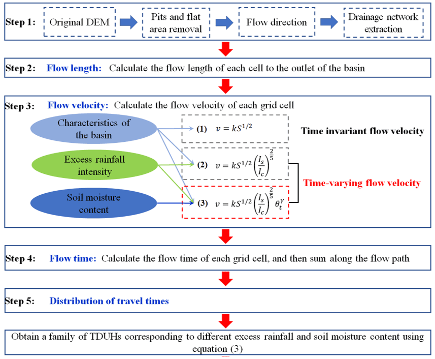
Figure 2Schematic diagram of the DUH method considering time-varying rainfall intensity and soil moisture content, in which Eqs. (1), (2) and (3) are the time-invariant flow velocity, time-varying flow velocity considering excess rainfall intensity and time-varying flow velocity considering both excess rainfall intensity and soil moisture content. The unit hydrograph derived from the three flow velocity equations corresponds to DUH, TDUH and the TDUH-MC method respectively.
The steps of the DUH method are summarized as follows:
-
The drainage network based on the advanced DEM preprocessing method is identified. More details can be found in Grimaldi et al. (2012).
-
Estimate the flow path, which is measured for each grid cell along the flow directions to the basin outlet.
-
Calculate the flow velocity based on watershed characteristics and the spatial–temporal distribution characteristics of rainfall. Several flow velocity formulas are commonly used for deriving the spatially distributed unit hydrograph, such as Manning's formula (Chow et al., 1988), the SCS formula (Haan et al., 1994), the Darcy–Weisbach formula (Katz et al., 1995), and the uniform flow equation by Maidment et al. (1996).
-
To compute the total travel time τi of flow from each cell i to the outlet, we added travel times along the Ri cells belonging to the flow path that starts at that cell, given by Eq. (11) (Muzik, 1996). The travel time for each grid cell can be calculated by Eq. (12):
where Δτi is the retention time in grid cell i, τi is the total travel time along the flow path in grid cell i and Li is the grid cell size. Travel length in a specific grid cell is the cell size Li when the rasterized flow is flowing along the edges of the grid, whereas the travel length is when it is flowing diagonally.
-
Develop a cumulative travel time map of the watershed based on cell-by-cell estimates for hillslope velocities. The cumulative travel time map is further divided into isochrones, which can be used to generate a time–area curve and the resulting unit hydrograph (Kilgore, 1997).
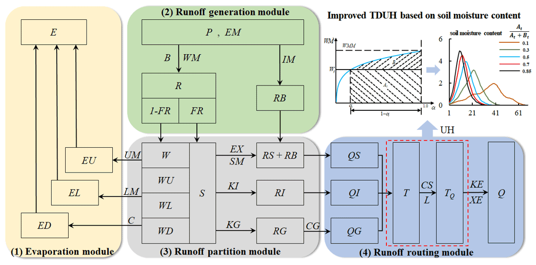
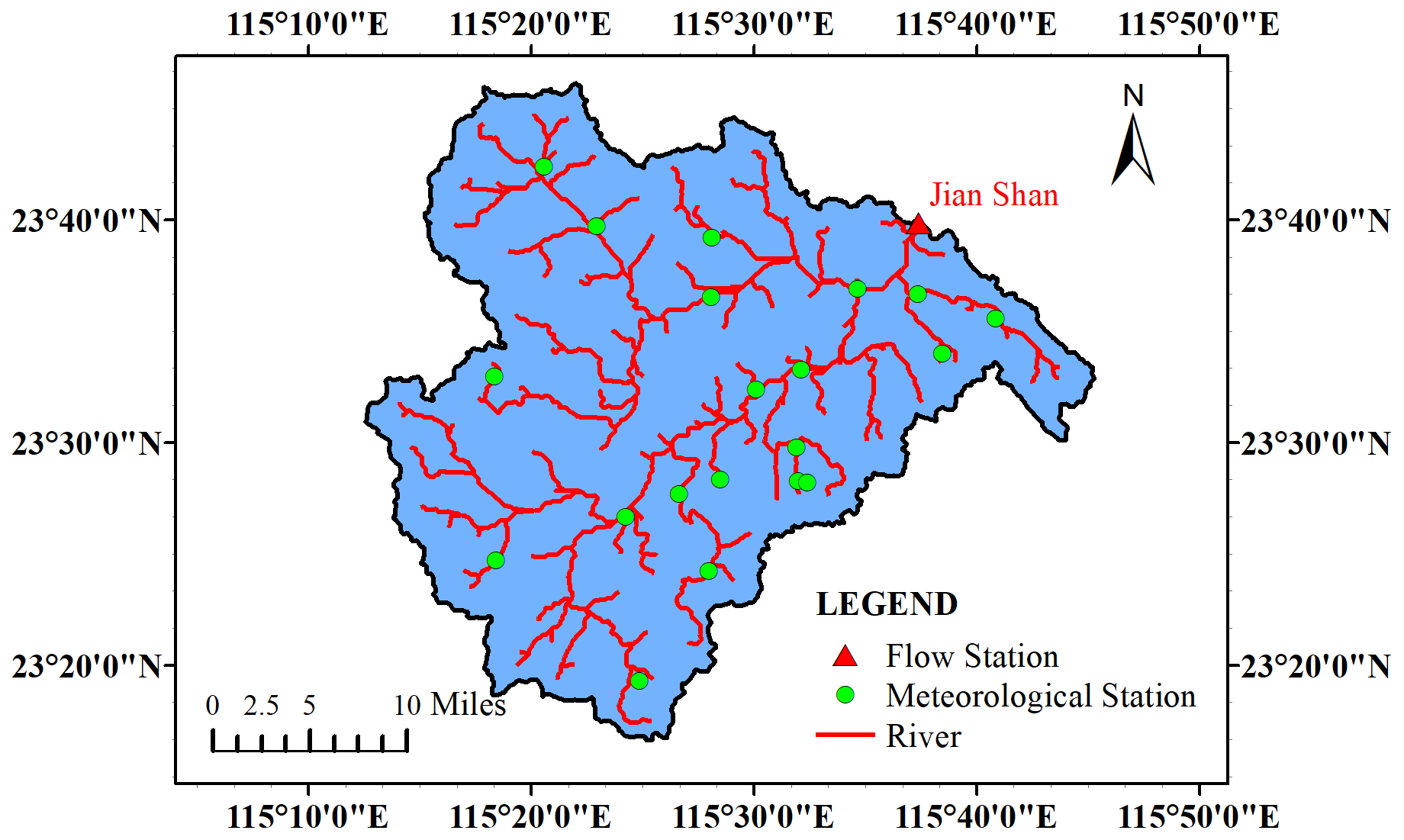
Figure 4Locations of meteorological stations and gauging stations in the Qin River basin.
The Xinanjiang (XAJ) model was used for the calculation of excess rainfall in this study. It is a conceptual hydrologic model proposed by Zhao et al. (1980) for flood forecasts in the Xinan River basin. The XAJ model has been widely used in humid and semi-humid watersheds all over the world (Zhao, 1992). It mainly consists of four modules, namely the evapotranspiration module, runoff generation module, runoff partition module and runoff routing module (Zhou et al., 2019). Usually, a large watershed is divided into several sub-basins to capture the spatial variability of underlying surface, precipitation, and evaporation. In each sub-basin, the inputs of the XAJ model are the average areal rainfall as well as evaporation, and the output is streamflow. The schematic diagram of the XAJ model is shown in Fig. 3.
First, for the evapotranspiration module, the soil profile of each sub-basin is divided into three layers, the upper, lower and deeper layers, and only when water in the layer above it has been exhausted does evaporation from the next layer occur. Second, for runoff generation in the XAJ model, a catchment is divided into two parts by the percentage of impervious and saturated areas, namely pervious and impervious areas, respectively. Since the soil moisture deficit is heterogeneous, runoff distribution is usually nonuniform across the basin. Thus, a storage capacity curve was adopted by the XAJ model to accommodate the nonuniformity of soil moisture deficit or the tension water capacity distribution. Third, the runoff partition in the XAJ model divides the total runoff into three components by a free reservoir, which consists of surface runoff (RS), interflow runoff (RI) and groundwater runoff (RG). More details can be found in Zhao et al. (1980).
Finally, the SUH was selected as the runoff routing approach in the XAJ model. Specifically, the Nash instantaneous unit hydrograph model (Nash, 1957) was used to derive the SUH in this study. For the Nash IUH model, a catchment was assumed to be made up of a series of n identical linear reservoirs, each with the same storage constant K. The magnitudes of n and K were estimated based on the observed excess rainfall hyetograph and corresponding direct runoff hydrograph using the method of moments. Details can be found in Singh (1988) and Chow et al. (1988).
The Muskingum method was employed to produce streamflow from each sub-basin to the outlet of the entire basin. For the SUH, the basin was taken as a whole. The parameters of the Muskingum method, including the Muskingum time constant KE and Muskingum weighting factor XE, were calibrated with those of the XAJ model. The Shuffled Complex Evolution Algorithm (SCE-UA) method was used to calibrate the parameters of XAJ model (Chu et al., 2009; Moghaddam et al., 2016). For the DUH, the basin was divided into several sub-basins. Since natural rivers are multiple inflow–single outflow runoff systems with different travel times from the sub-basins to the outlet, we adopted the physical and numerical principles established by Cunge to calculate the routing parameters of the Muskingum method, which is suitable for ungauged watersheds (Ponce et al., 1996). The Muskingum parameters for each sub-basin were determined based on flow and channel characteristics, such as the top width of the river, wave celerity, reach length and reach slope, as described in Chow (1959) and Wilson and Ruffin (1988).
The Qin River basin and Longhu River basin were selected as two case study watersheds. One is a large watershed, and the other is a small watershed. The applicability of the TDUH-MC method to different size watersheds was verified, and parameter sensitivity analysis was done to evaluate the performance of the TDUH-MC method (Chen et al., 2022a).
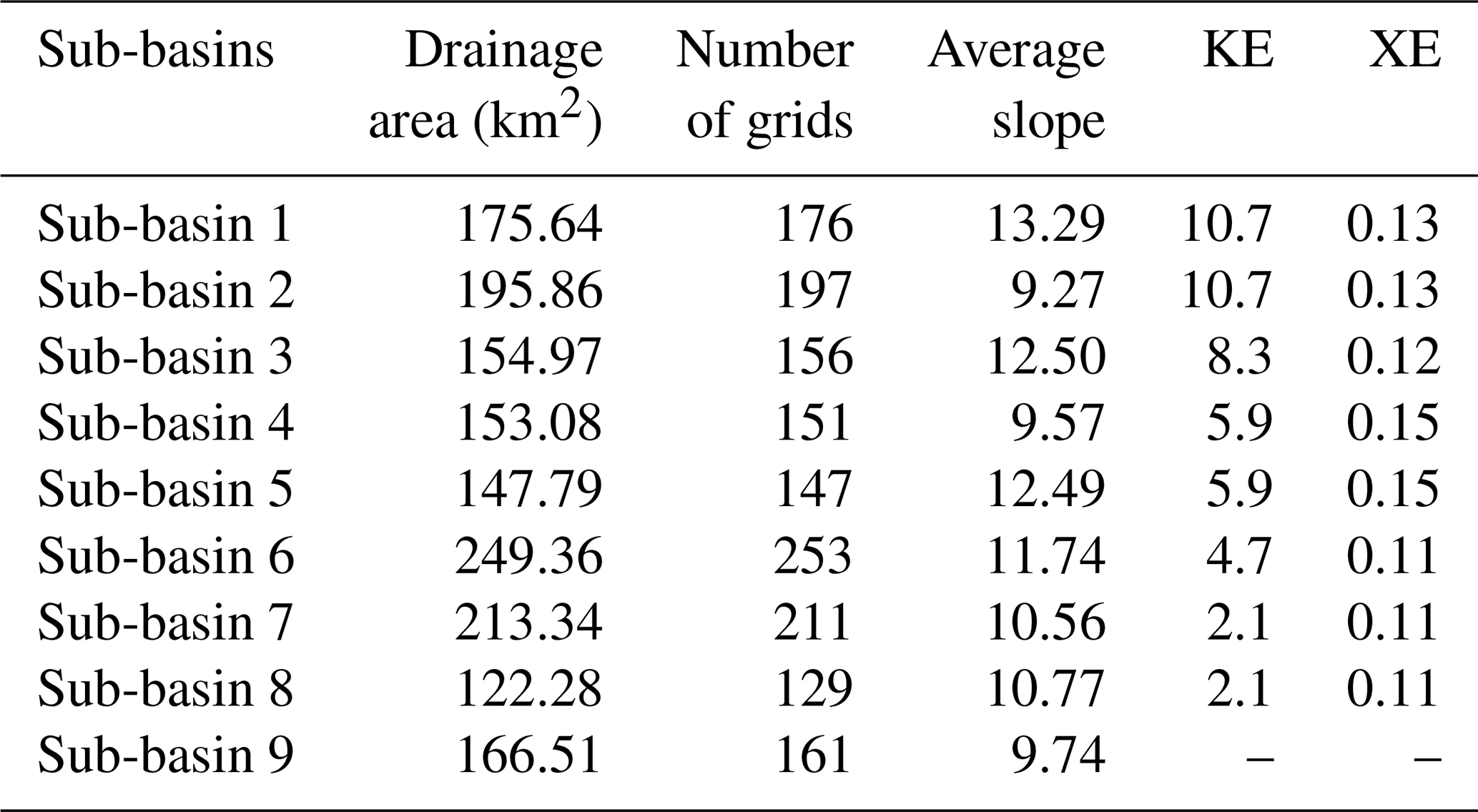
The Qin River is a tributary of the Mei River, which originates from Guangdong Province, China. The river is 91 km long, with a basin area of 1578 km2. The mean slope of the basin is 1.1 ‰. There are 21 meteorological stations and 1 flow station (the Jianshan station) in the basin, as shown in Fig. 4. Using the DEM data of the Qin River basin, the whole basin was divided into nine sub-basins, namely sub-basins 1–9 from upstream to downstream, as shown in Fig. 5. Details of each sub-basin are given in Table 1.
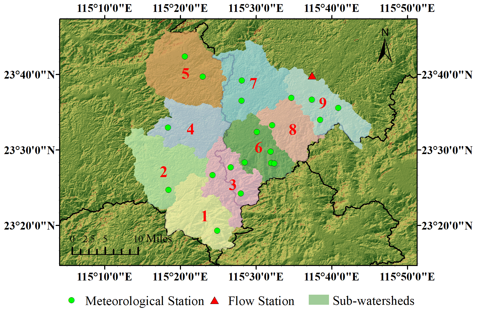
Figure 5Sub-basins of the Qin River basin. (Note that the satellite images for the study area are available at http://www.gscloud.cn, last access: 18 November 2020.)
The Longhu River basin is a small watershed, which has a drainage area of 102.7 km2, located in Guangdong Province, China. The length of the river is 17.4 km.
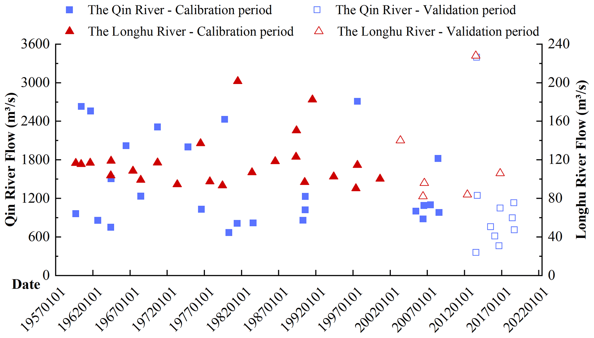
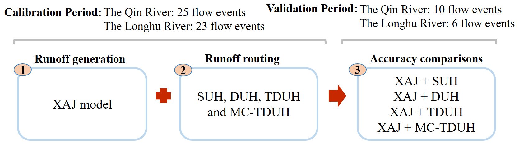
The rainfall and evaporation data from meteorological stations for the two basins were collected from 1959 to 2018, and the simultaneous hourly runoff data for the Jianshan Station and Longhu Station were collected as well. A total of 64 isolated storms with the observed runoff responses from 1959 to 2018 were selected to calibrate and verify the established model, of which 35 events were collected from the Qin River basin and 29 from the Longhu River basin. In total, 25 and 23 flow events were used for model calibration in the Qin and Longhu River basins respectively, and 10 and 6 flow events were used for model validation in the two basins.
The statistics of flow events used for model calibration and validation are shown in Fig. 6. The average peak flows of the two basins were 1311 and 118 m3 s−1, and the average flood durations were about 50 and 13 h, respectively. The antecedent precipitation was calculated based on the daily recession coefficient of water storage in the basin.
5.1 Calibration of parameters
5.1.1 Model calibration
The runoff generation model (XAJ model) and the routing model were calibrated separately in this study. First, the SUH and several distributed unit hydrographs (DUH, TDUH and MC-TDUH) were derived. Second, the Shuffled Complex Evolution Algorithm (SCE-UA) method, developed by the University of Arizona (Duan et al., 1992), was used to optimize the XAJ model parameters (Vrugt et al., 2006; Beskow et al., 2011; Zhou et al., 2019). The SUH was selected as the runoff routing method. As the SUH was derived from observed rainfall and runoff, the flow routing model corrected some inconsistencies of the hydrological model. Therefore, the parameters of excess runoff were calibrated. Third, the performances of XAJ + SUH and XAJ + DUHs (DUH, TDUH and MC-TDUH) were compared. Since the XAJ model parameters were determined by combining with SUH routing method, this calibration method would be more inclined to optimize the performance of XAJ + SUH model. When combined with other confluence models, the accuracy of results may be affected to some extent. The schematic of the calibration procedure is given below.
The steps of parameter calibration can be summarized as follows:
-
The XAJ model was used to calculate the excess rainfall, in which the SUH derived from observed runoff was selected as the runoff routing method. The SCE-UA method was used to optimize the XAJ model parameters in this study. In total, 25 and 23 flow events in the Qin River basin and Longhu River basin were used for the calibration of the XAJ + SUH model.
-
The SUH was derived using 25 and 23 flow events in the Qin River basin and Longhu River basin, respectively. The DUH, TDUH and MC-TDUH were derived, based on physical characteristics and rainfall intensities of the watersheds. The parameters' determination method is given in Sect. 5.1.3.
-
Since the objective of this study was to propose a new flow routing method, the runoff production model and its parameters were not changed in order to discuss the performance of flow routing models. The XAJ model with calibrated parameters in Step (1) and DUH, TDUH as well as MC-TDUH determined in Step (2) were used for the validation period. A total of 10 and 6 flow events of the two basins were then used for the validation of the XAJ + (SUH, DUH, TDUH and MC-TDUH) model.
The Nash–Sutcliffe efficiency (ENS) (Nash and Sutcliffe, 1970; Chen et al., 2015), the Kling–Gupta efficiency (EKG) (Gupta et al., 2009) and the root-mean-squared error to standard deviation ratio (RSR) were chosen as criteria. Moreover, the new aggregated objective function (Brunner et al., 2021) targeted at optimizing flow characteristics was composed of these three metrics, in which EKG focuses on high flows (Mizukami et al., 2019), log(ENS) emphasizes low flows and RSR quantifies volume errors. A similar method has been used by Chen et al. (2022b, c). Three metrics and the aggregated objective function are expressed by
where is the observed discharge at time t, is the simulated discharge at time t, is the mean of observed discharge, T is the duration of the flow event, r is the correlation coefficient between observed and simulated floods, σs and σo are the standard deviation values for the simulated and observed responses, respectively, and μs and μo are the corresponding mean values.
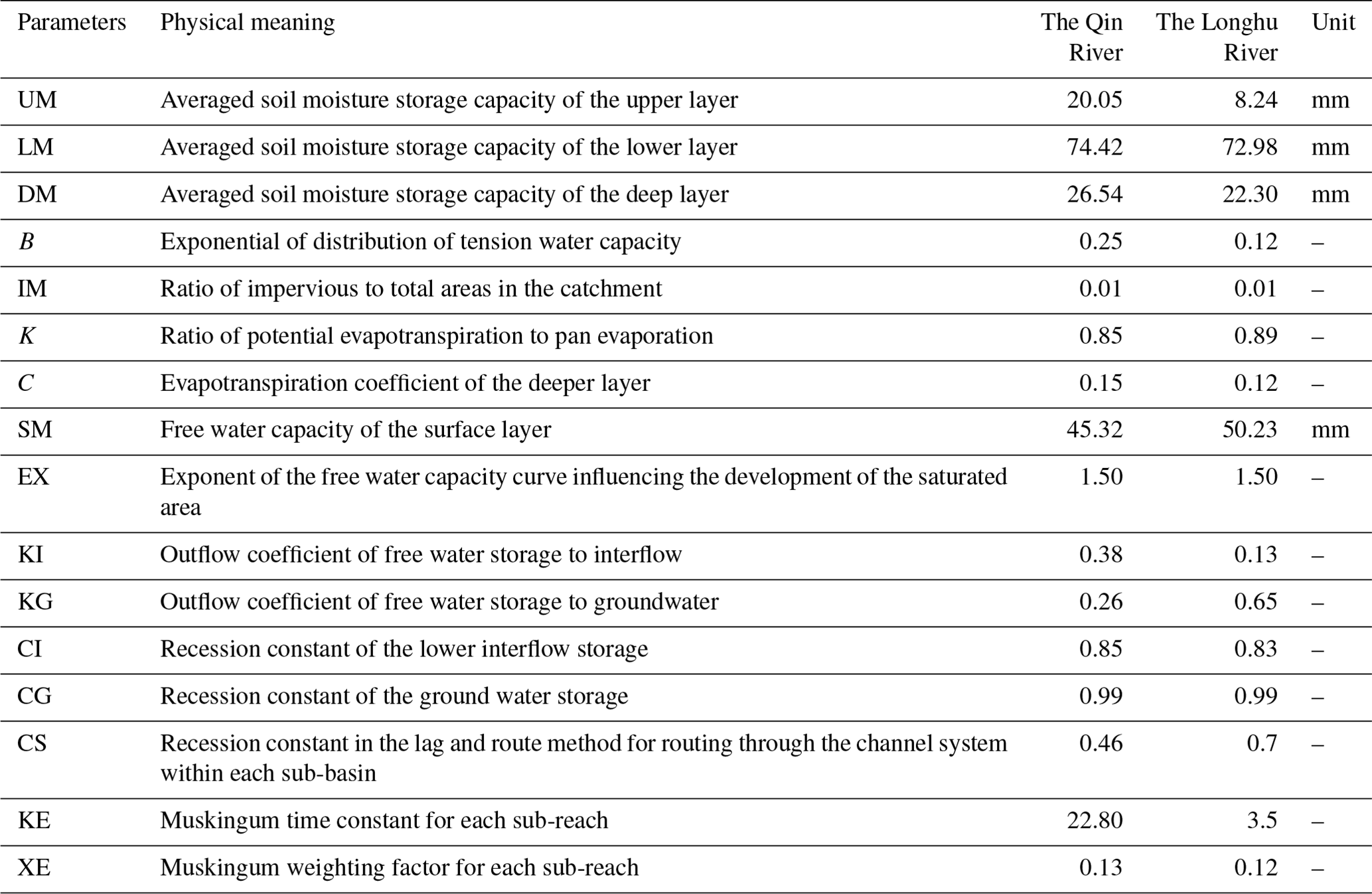

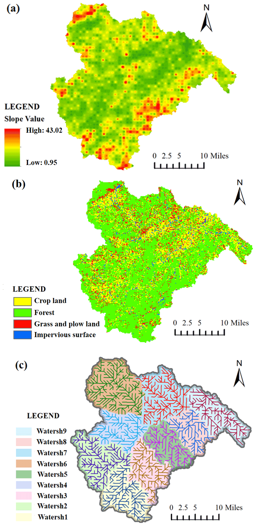
Figure 8(a) Slope distribution, (b) land types and (c) rasterized flow direction of the Qin River basin.
5.1.2 Calibrated parameters of runoff generation using the XAJ model
Since the Qin River basin and Longhu River basin are in a humid area of southern China, the saturation-excess mechanism with three-source runoff separation of the XAJ model was adopted to calculate excess rainfall. The initial condition of the XAJ model was considered by calculating the antecedent precipitation index before each flow event (Linsley et al. 1949). The synthetic unit hydrograph, derived by historical rainfall-runoff data, was used for flow routing in the process of model calibration. The time interval was 1 h. Several studies have shown that UH which is derived by considering antecedent soil moisture is more consistent than UH which ignores that (Yue and Hashino, 2000; Nourani et al., 2009). Therefore, the antecedent precipitation was calculated and considered in this study. In order to obtain the SUH, we defined excess rainfall and separated direct runoff and baseflow hydrographs in advance. The final SUH used for calibration is the average value deduced by multiple historical flow events. The parameter n of the Qin River basin and Longhu River basin was 4 and 3, and the parameter K for the two basins was 3.4 and 2.1, respectively. Then, the flow peak, flow volume and the occurrence time of flow peak are three main basic elements for describing the flow hydrograph, and Eq. (16) was used as the aggregated objective function. The average Nash–Sutcliffe efficiency, relative flood peak error and peak occurrence time error obtained in the calibration period of the XAJ model were 0.84 %, 10.4 % and 4.96 h, respectively, for the Qin River basin. Accordingly, for the Longhu River basin, they were 0.86 %, 8.81 % and 2.75 h respectively, indicating a good performance of the XAJ model. Detailed information on the calibrated parameters of the XAJ model is shown in Table 2.
5.1.3 Calibrated parameters of the TDUH-MC flow routing method
As mentioned in Sect. 2.2, the core of the DUH is the calculation of the grid flow velocity. As shown in Eq. (3), the parameters that needed to be calibrated were k, S, Ic and γ, in which Ic was determined using hourly mean rainfall intensity and flow forecast of the target basin. For the Qin River basin, Ic was set at 20 mm h−1 because the mean rainfall intensity of multiple flows was about 20 mm h−1, and this parameter was 10 mm h−1 for the Longhu River basin. Additionally, parameter γ reflected the influence of soil moisture content in unsaturated regions on flow velocity. The smaller the parameter γ was, the smaller the influence of soil moisture content on the flow velocity was. When the value of γ was equal to 1, the flow velocity of grid cell was proportional to the soil moisture content factor θt. The parameter γ of soil moisture content was determined to be 0.5 to reflect the influence of soil moisture content on the flow velocity for the two basins. Furthermore, sensitivity analysis for this parameter was conducted in Sect. 5.6. In order to get the grid cell slope S, the slope distribution of the study areas was obtained from the DEM data of the target basin. Figure 8a plots the slope distribution of the Qin River basin. Parameter k is the velocity coefficient, which was determined based on different underlying surface types or different flow states (Ajward and Muzik, 2000). Parameter k changed with different land types, and the k values used in this study are given in Table 3. The land types of the Qin River basin are shown in Fig. 8b. Then the k values of each grid cell were determined by combining Fig. 8b and Table 3.
The grid flow velocity was calculated by Eq. (3) with the above parameter values. Then, the flow travel time was determined by Eqs. (11) and (12). It is noteworthy that the raster size of the Qin River basin was divided into 1 km × 1 km, and the rasterized flow direction of each sub-basin is shown in Fig. 8c. For the Longhu River basin, the difference was that its cell size was divided into 30 m × 30 m to evaluate the performance of the TDUH-MC method in this small watershed.
5.2 Calculation of the TDUH-MC
After determining the parameters, flow routing was calculated based on the proposed DUH, considering the time-varying soil moisture content. In order to improve the effectiveness of the routing method, the rainfall intensity and soil moisture content parameters were discretized. Then, a simplified TDUH considering time-varying soil moisture content and the TDUH were obtained in a certain range of rainfall intensities or soil moisture contents; these ranges are presented in Tables 4 and 5. To evaluate the performance of the TDUH-MC method, the traditional SUH, DUH and TDUH methods were used for comparison.
Table 4The ratio of It to Ic of each period corresponds to the discrete rain intensity Is.
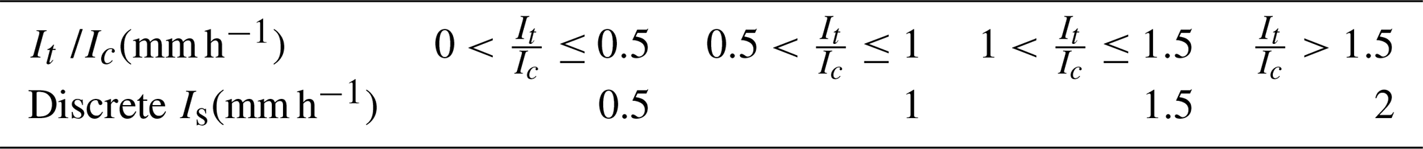
Table 5The soil moisture content θt of each period corresponds to the discrete soil moisture content θs.

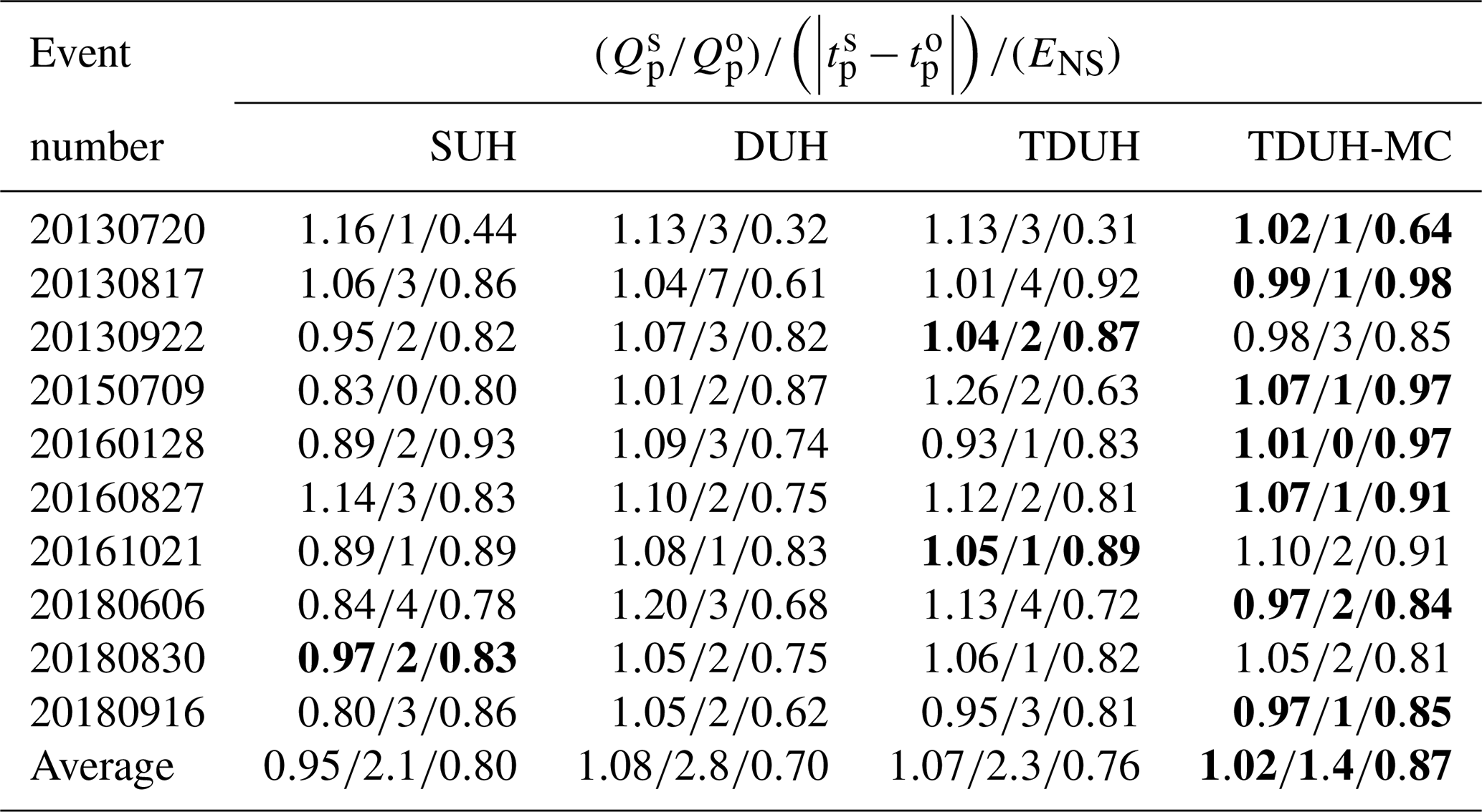
Table 6Comparison of four routing methods for the Qin River basin. The values in bold mean the result performed the best among the four methods.
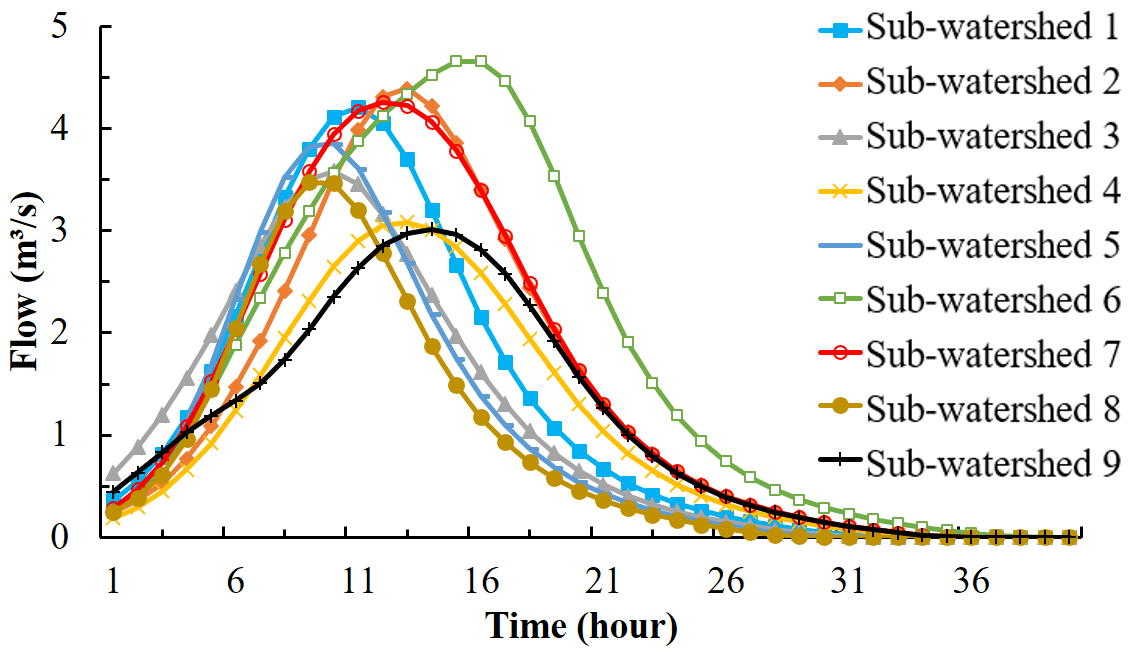
The DUH without considering rainfall intensity and soil moisture was obtained using Eq. (1). Results of the DUH for each sub-basin of the Qin River basin are shown in Fig. 9. There is only one DUH for a specific sub-basin due to the simplification of the underlying surface, such as slope and land covers. The differences among the DUHs were mainly reflected in flow peaks and their occurrence times. It can also be seen from Fig. 9 that the peak of DUHs in sub-basins 4 and 6 was significantly lower than in others. The reason may be that the smaller mean slope values of sub-basins 4 and 9 lead to lower flow velocity, resulting in a lower peak of the DUH.
The TDUHs corresponding to different rainfall intensities of nine sub-basins are shown in Fig. 10. It can be seen from Fig. 10 that different rainfall intensities corresponded to different TDUHs. The increased rainfall intensity led to higher peak and earlier peak occurrence time of the UH. This is because a larger rainfall intensity caused a larger flow velocity according to Eq. (2). In the practical use of TDUH, the UHs need to be selected according to rainfall intensities.
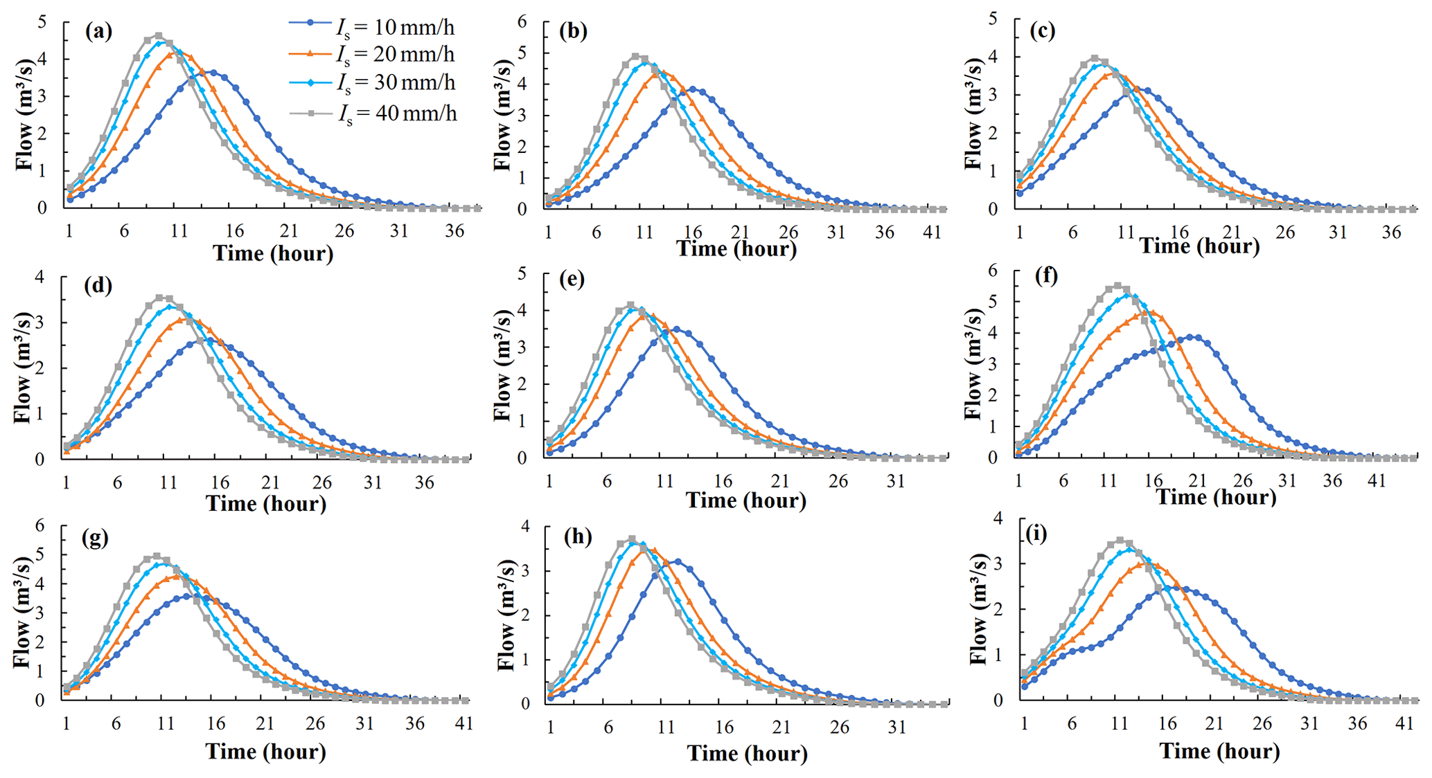
Figure 10The TDUH for the Qin River basin. (a) Sub-basin 1. (b) Sub-basin 2. (c) Sub-basin 3. (d) Sub-basin 4. (e) Sub-basin 5. (f) Sub-basin 6. (g) Sub-basin 7. (h) Sub-basin 8. (i) Sub-basin 9.
The TDUH of each sub-basin was further divided according to the soil moisture content. The TDUHs considering soil moisture contents of sub-basin 1 are shown in Fig. 11. Obviously, under the same rainfall intensity, the soil moisture content was of great importance to the shape, peak value and duration of the TDUH. Specifically, when the proportion of soil moisture content θt increased, the TDUH-MC method considering soil moisture content was accompanied by a steeper rising limb, a higher peak and shorter duration. After the whole basin was saturated, the TDUH considering the soil moisture content was the same as the TDUH.
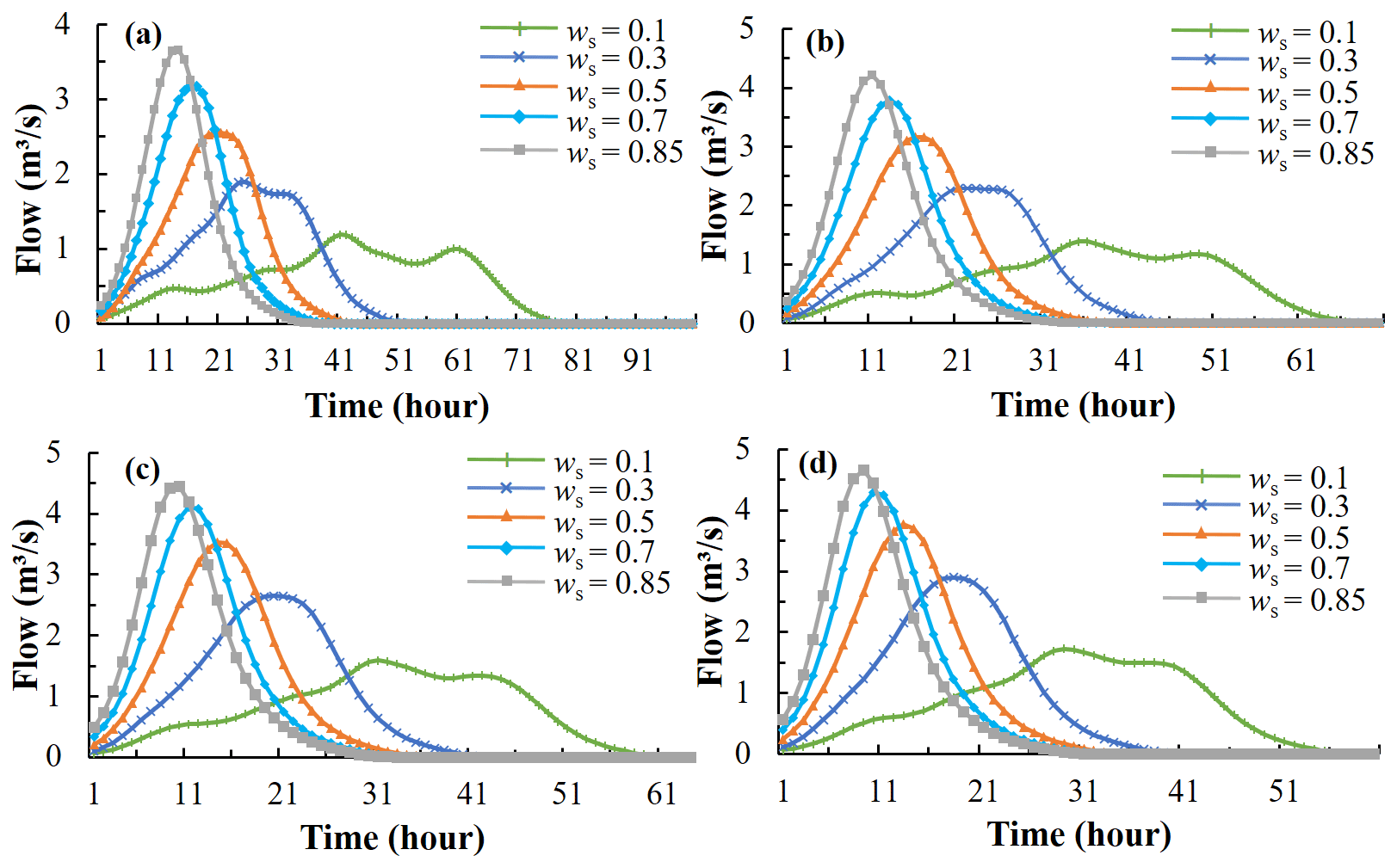
Figure 11The TDUH considering soil moisture content for sub-basin 1 of the Qin River basin. (a) Is=0.5. (b) Is=1. (c) Is=1.5. (d) Is=2.
Similarly, the TDUHs considering the soil moisture content for the Longhu River basin are shown in Fig. 12. The grey line in Fig. 12b is the DUH, where Is is equal to 1, and ws is 0.85. Four grey unit hydrographs in Figs. 12a to d make up the TDUH without considering the soil moisture content.
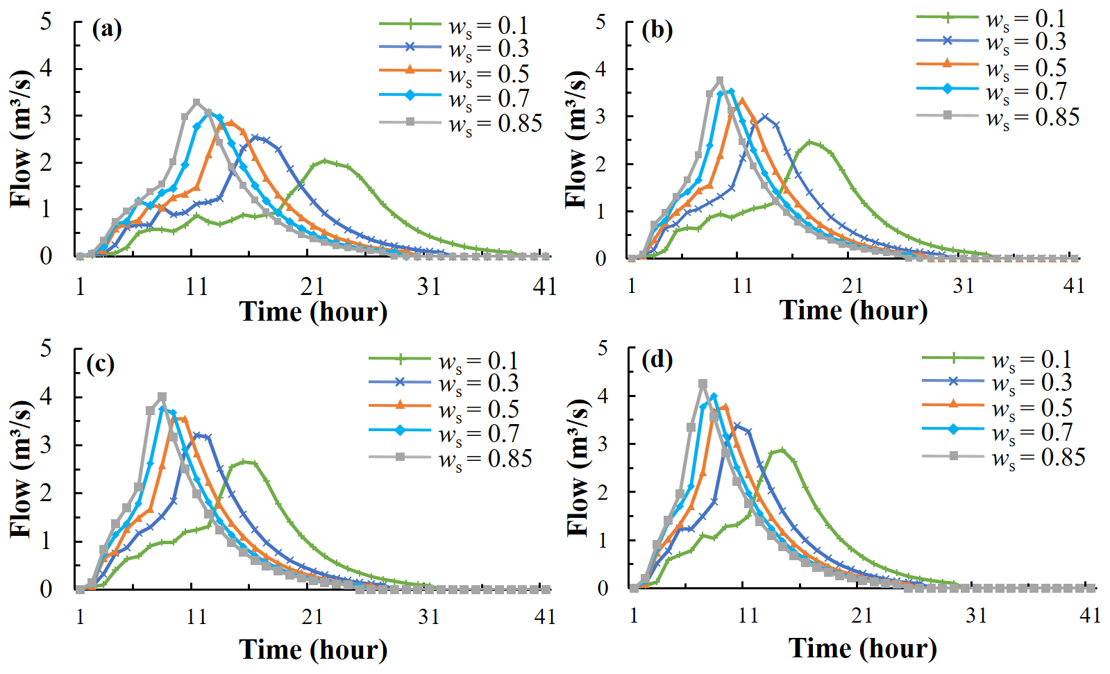
Figure 12The TDUH considering soil moisture content for the Longhu River basin. (a) Is=0.5. (b) Is=1. (c) Is=1.5. (d) Is=2.
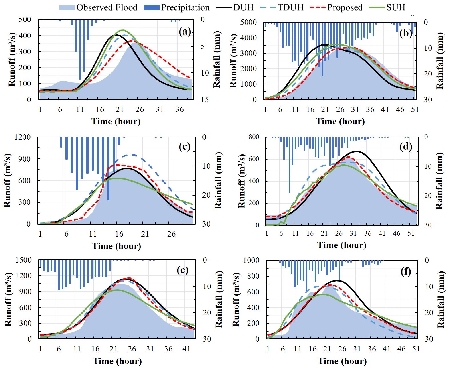
Figure 13Comparison of flow hydrographs obtained by the four methods. (a) Flow event no. 20130720. (b) Flow event no. 20130817. (c) Flow event no. 20150709. (d) Flow event no. 20160128. (e) Flow event no. 20161021. (f) Flow event no. 20180916.
5.3 Comparisons of flood routing methods
The runoff generation module of the calibrated XAJ model was used to calculate the excess rainfall, and the SUH, DUH, TDUH and improved TDUH considering soil moisture content were employed for flow routing calculations, respectively. The Muskingum parameters for each sub-basin are given in Table 1. Dozens of flow events were applied for model validation. Simulated results of the four methods for the Qin River basin are shown in Table 6. Three criteria were used for model performance evaluation, which included the Nash–Sutcliffe efficiency (ENS), the ratio between the simulated and observed peak discharges (), and the error between simulated and observed times to peak . The ratio between simulated and observed peak discharges of the TDUH-MC method ranged from 0.97 to 1.10. The average peak occurrence time error of the TDUH-MC method was 1.4 h, which was the smallest among the four methods, and the mean ENS coefficients of the 10 flow events for validation were above 0.8. Figure 13 shows the flow hydrographs of the four routing methods for part of the flow events (event no. 20130720, 20130817, 20150709, 20160128, 20161021 and 20180916). It is demonstrated that the TDUH-MC method outperformed the remaining three routing methods.
In addition, the forecast results of six flow events in the Longhu River basin using the SUH, DUH, TDUH and the TDUH-MC method are presented in Table 7. Results of the TDUH-MC method generally showed the best performance, which also verified the TDUH-MC formula for the small watershed. In general, the TDUH-MC method was capable of better simulation in this watershed than in the Qin River basin.
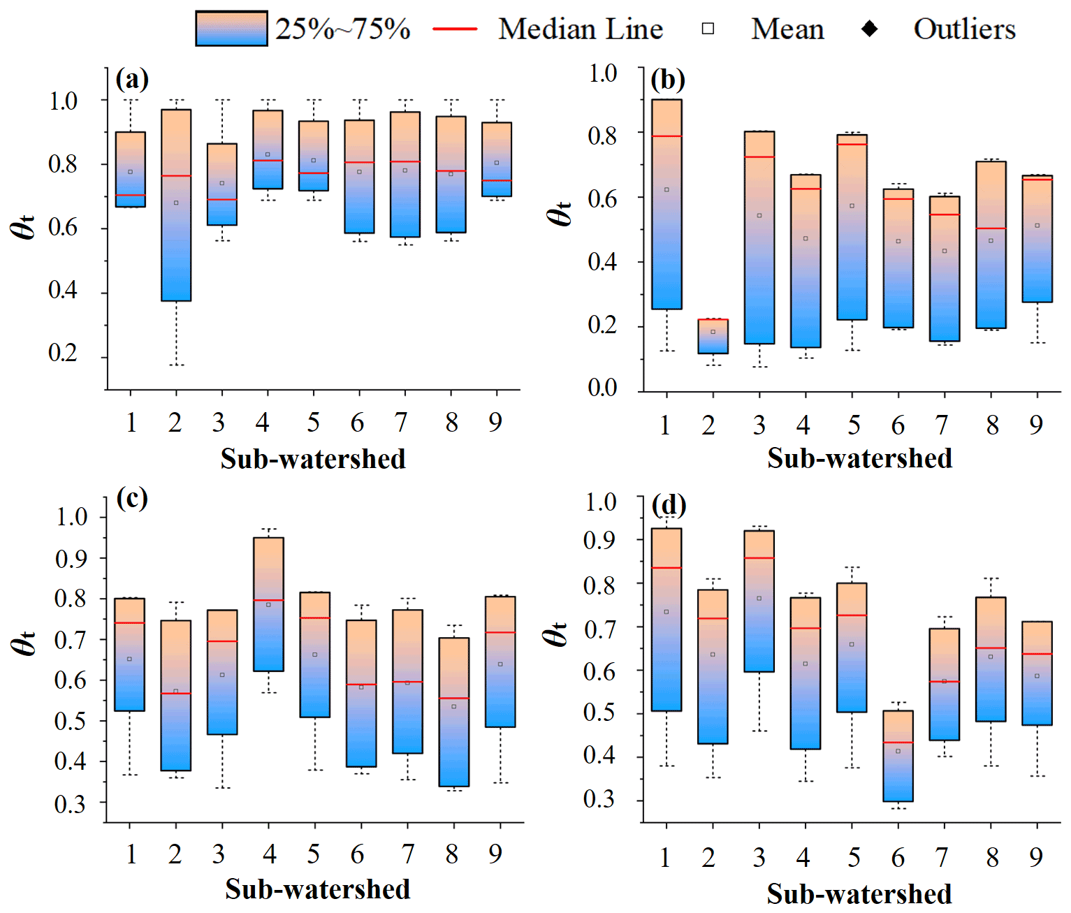
Figure 14Distributions of time-varying θt at different times in each sub-basin using the TDUH-MC method. (a) Flow event no. 20130817. (b) Flow event no. 20150709. (c) Flow event no.20160128. (d) Flow event no. 20180916. θt represents the ratio of current soil moisture storage to the corresponding maximum soil moisture capacity in the unsaturated region.
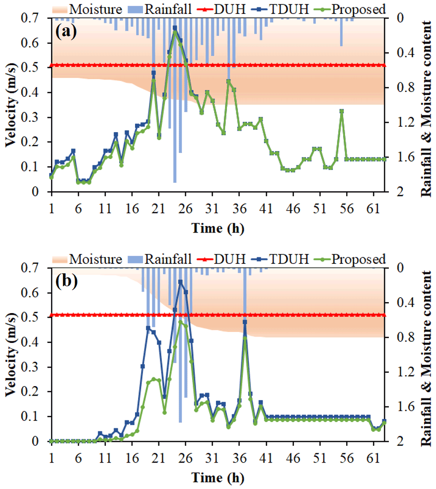
Figure 15Time-varying velocity values of a grid cell in different storm events. (a) Time-varying velocity in storm event no. 20130817. (b) Time-varying velocity in storm event no. 20150709. The rainfall content is Is, and the soil moisture content is θs.
Table 7Comparison of four routing methods for the Longhu River basin. The values in bold mean the result performed the best among the four methods.

For flow event no. 20161021, the simulation result of the TDUH-MC method was basically consistent with that of the TDUH method. This was because the antecedent rainfall was close to saturation under this flow event. As a result, the TDUH-MC method performed the same as the TDUH method when the watershed was saturated. For flow event no. 20180916, the simulation accuracy of the TDUH-MC method was lower than that of the TDUH. The possible reason for the inaccurate flow simulation is that the antecedent rainfall was relatively small. Because the runoff generation was not dominated by the saturation excess, it was not appropriate to calculate runoff with the XAJ model.
5.4 Influence of time-varying soil moisture content on flow forecasts
In order to evaluate the influence of time-varying soil moisture content on flow forecasts, three typical flow forecast results of the TDUH-MC method were selected for comparison in the Qin River basin. Specifically, compared with the forecasting results using TDUH, results of flow event no. 20130817 using the TDUH-MC method were relatively similar, results of flow events no. 20150709 and 20160128 had a better performance, and results of flow event no. 20180916 were poor. Their corresponding temporal evolution of soil moisture content in unsaturated regions was obtained. The box-and-whisker plots of soil moisture contents of all sub-basins for flow events no. 20130817, 20150709, 20160128 and 20180916 are shown in Fig. 14. It can be seen from Fig. 14 that the soil moisture content of each sub-basin was initially low, and then the soil moisture content of the sub-basin gradually increased. Meanwhile, it was obvious that θt was hard to reach the maximum value. For all flow events, nine sub-basins eventually reached saturation only under the condition of flow event no. 20130817. The mean values of θt for flow events no. 20150709, 20160128 and 20180916 ranged from 0.5 to 0.8, and the soil moisture content did not reach the maximum during the flow events. As shown from the observed flow in Fig. 13, the peak discharge of the flow event no. 20130817 was larger than those of other flow events, reaching 3500 m3 s−1, which meant that the watershed more probably reached saturation during the flow period.
As discussed in Sect. 5.3, results of flow event no. 20130817 using the TDUH-MC routing method showed the same behavior as did TDUH. This was because the simulation performance of the TDUH-MC method considering time-varying soil moisture content was the same as that of TDUH when the soil moisture content was closer to 1. Additionally, the forecast results of flow events no. 20150709 and 20160128 with the TDUH-MC routing method were obviously better than those of DUH and TDUH. The reason can be summarized as follows. The mean values of θt ranged from 0.5 to 0.6 for the two flow events, and the θt values were initially low as shown in Fig. 14. Thus, the soil moisture content had a significant impact on the shape of the hydrograph. For flow event no. 20180916, the sub-basins did not reach a global saturation, and the time-varying values of θt were generally high, which led to lower flow velocity than in the TDUH method. The peak occurrence times of unit hydrographs used for runoff routing calculations were in general later, leading to a lag time between maximum rainfall intensity and peak discharge for the forecast result of flow event no. 20180916.
5.5 Comparison of velocity calculated by three DUH methods
The routing method considering both time-varying rainfall intensity and soil moisture content was more accurate as discussed in Sect. 5.3. To evaluate the effect of time-varying soil moisture content on flow velocity, we selected a grid cell in sub-basin 3, in which slope and land type parameters were constant. Then, the flow velocity was calculated under different storm conditions. The storm events no. 20130817 and 20150709 were selected and compared because storm event no. 20130817 had a high intensity and long duration, and storm event no. 20150709 had a short period of heavy rainfall. Thus, soil moisture contents during the two storm events were significantly different. Figure 15 shows the time-varying velocity values of a grid cell for storm events no. 20130817 and 20150709. For the two storm events, the mean velocity of the DUH method was the largest among the three methods, followed by the TDUH method. The velocity calculated by the TDUH-MC method considering soil moisture content was the smallest. The velocity of DUH method was constant in the two storms, and that of the TDUH method varied with the change of excess rainfall. Meanwhile, the flow velocity of the TDUH-MC method was not only dominated by rainfall intensity, but was also related to soil water content.
For storm event no. 20130817, the initial soil moisture content was large, and it reached the maximum rapidly. The flow velocity of the TDUH-MC method was slightly smaller than that of the TDUH method at the initial stage of storm events. When the whole basin reached saturation, the flow velocities of the two methods became equal. Therefore, the differences between hydrographs were small when using the TDUH method and the TDUH-MC method for flow routing calculation, which led to similar forecast results.
For storm event no. 20150709, the initial soil moisture content was small, and the entire basin could not reach saturation after the rainstorm. Therefore, the grid velocity in the early stage of the storm was greatly affected by the soil moisture content. In the later stage of the rainstorm, θt of the watershed did not reach the maximum but was nearly close to 1. Thus, the impact of later soil moisture content on the flow velocity was small. From the above analyses, it can be concluded that the shape and duration of the unit hydrograph were mainly related to the soil moisture content at the initial stage of a storm, and when the watershed was approximately saturated, the grid flow velocity was mainly dominated by the excess rainfall.
5.6 Sensitivity analysis for the TDUH-MC method
A sensitivity analysis for the proposed formula was done in the Longhu River basin. The improved method only has two additional parameters, compared with the current model. The objective of this study was to explore the influence of the soil moisture content factor on the performance of the DUH model. Parameter γ in Eq. (3) significantly affected the significant degree of influence over how large soil moisture content will be. Thus, sensitivity analysis for parameter γ was necessary. A specific grid cell in the Longhu River basin was taken as an example, where the slope of the grid cell was set to 0.22 m m−1. The coefficient of flow velocity k and the ratio of rainfall intensity to the reference rainfall intensity Is were assumed to be 1.5 m s−1 and 1, respectively. When parameter γ was 0.1, 0.5 and 1, respectively, the hillslope flow velocity values corresponding to different rainfall and soil moisture contents using the proposed formula are given in Fig. 16.
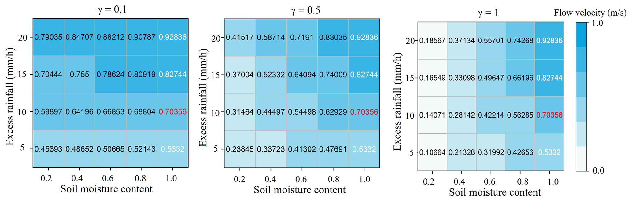
It can be seen from Fig. 16 that when θt was equal to 1, the proposed Eq. (3) turned to Eq. (2). The flow velocity values in the last column were the same and only changed with rainfall intensities. When It was equal to the reference rainfall Ic, Eq. (2) turned to Eq. (1), and the flow velocity was 0.704 m s−1. After introducing a soil moisture content factor into the flow velocity formula, the flow velocity values ranged from 0.107 to 0.928 m s−1 when γ was equal to 1. The flow velocity values were significantly different corresponding to different values of parameter γ. Thus, the parameter γ significantly affected the performance of the new routing method.
Moreover, the mean flow velocity of the Longhu River basin was calculated under different rainfall intensities (e.g., , 1, 1.5, 2, respectively). Figure 17 plots the theoretical curve of mean velocity and soil moisture content.
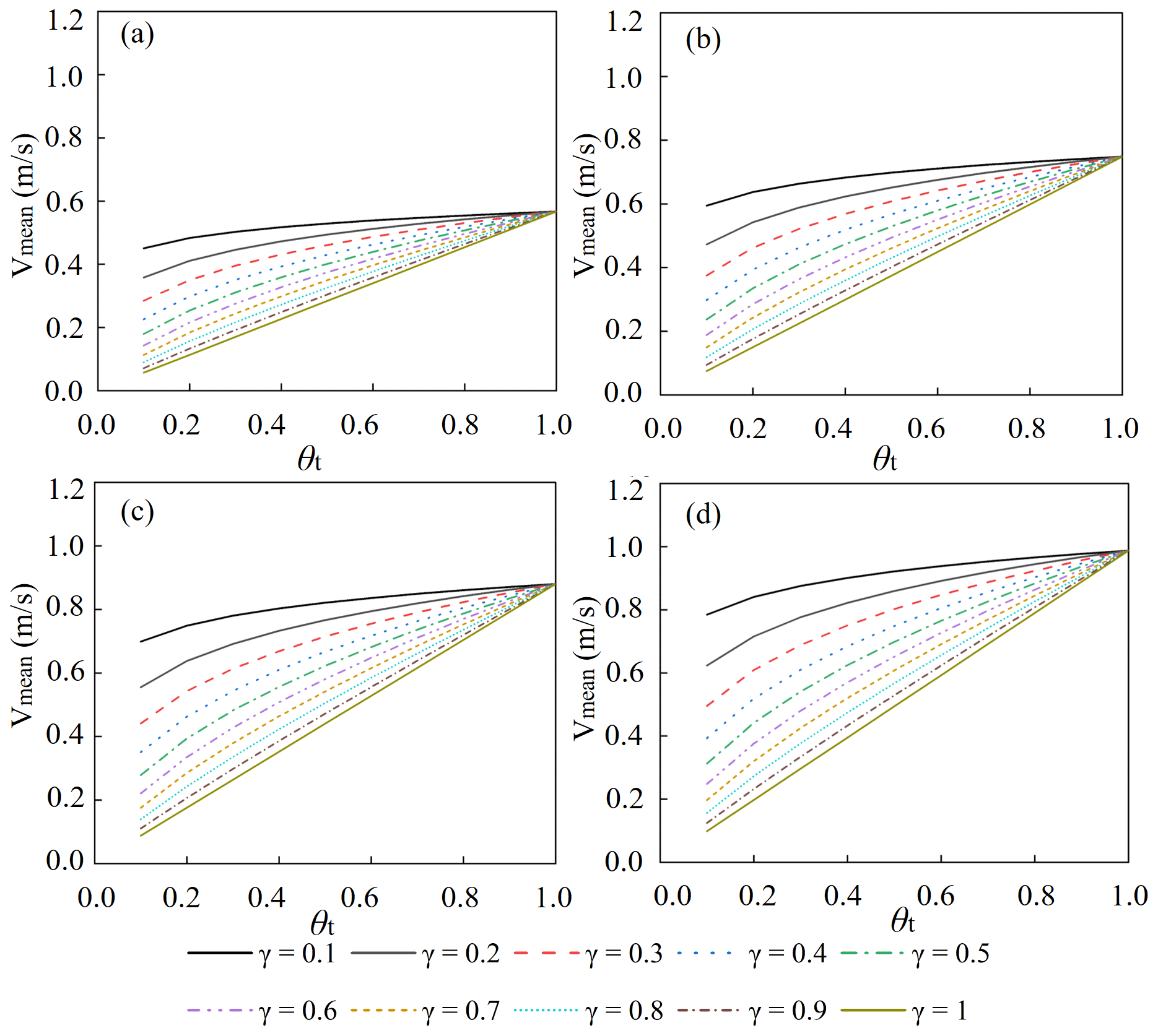
Figure 17The theoretical curve of mean velocity and soil moisture content for the Longhu River basin. (a) . (b) . (c) . (d) .
Figure 17 reveals that the mean flow velocity ranged from 0.6 to 1 under different rainfall intensities without considering the influence of soil moisture content. After introducing this new factor into the current flow velocity formula, the mean flow velocity was significantly influenced by exponent γ. In addition, when the soil moisture content exceeded 0.7, the variation range of mean flow velocity decreased sharply. Results showed that the influence of parameter γ on the flow velocity decreased gradually with the increase of soil moisture content.
An improved distributed unit hydrograph method considering time-varying soil moisture content was proposed for flow routing. The TDUH-MC method comprehensively considered the changes of time-varying soil moisture content and rainfall intensity. The response of the underlying surface to the soil moisture content was considered an important factor. The Qin River basin and Longhu River basin were selected as two case studies. The SUH, DUH, TDUH and TDUH-MC routing methods were used for flow forecasting, and simulated results were compared. The sensitivity analysis was conducted for parameter γ. The main conclusions can be summarized as follows.
-
The TDUH-MC runoff routing method, considering both time-varying rainfall intensity and soil moisture content, was proposed, and the influence of the inhomogeneity of runoff generation on the routing process was considered. It was found that the soil moisture content was a significant factor affecting the accuracy of flow forecast, especially in the catchment dominated by saturation-excess runoff, and the flow velocity increased gradually with more surface runoff after considering the soil moisture content in unsaturated regions.
-
The time-varying characteristics of the DUH can be further considered by introducing both rainfall intensity and soil moisture content into the flow velocity formula, which can effectively improve the accuracy of flow forecasts. Simulation hydrographs and criteria of the two case studies showed that the accuracy of the TDUH-MC method was the highest, followed by the SUH and TDUH methods and finally the DUH method.
-
The shape and duration of the improved TDUH considering soil moisture were mainly affected by rainfall intensity. Meanwhile, soil moisture content in the initial stage of a storm also played a significant role in the characteristics of the improved TDUH. When the watershed was approximately saturated, the grid flow velocity was mainly dominated by excess rainfall.
-
Results of sensitivity analysis showed that the accuracy of the TDUH-MC method was mainly affected by soil moisture content. The influence of parameter γ on the flow velocity decreased gradually with the increase of soil moisture content.
Due to the strict security requirements of departments, some or all data, models, or code generated or used in the study are proprietary or confidential in nature and may only be provided with restrictions (e.g., anonymized data).
LC conceived the original idea, and BY designed the methodology. PJ collected the data. BY developed the code and performed the study. BY, LC, HZ and VPS contributed to the interpretation of the results. BY wrote the paper, and LC and VPS revised the paper.
The contact author has declared that none of the authors has any competing interests.
Publisher’s note: Copernicus Publications remains neutral with regard to jurisdictional claims in published maps and institutional affiliations.
This research is supported by the National Key Research and Development Program of China (2021YFC3200400), the National Natural Science Foundation of China (51922047; 51879109), the Hubei Science Foundation for Distinguished Young Scholars (2020CFA101) and the Fundamental Research Funds for the Central Universities (2019kfyRCPY057).
This research has been supported by the National Key Research and Development Program of China (2021YFC3200400), the National Natural Science Foundation of China (51922047, 51879109), the Hubei Science Foundation for Distinguished Young Scholars (2020CFA101) and the Fundamental Research Funds for the Central Universities (2019kfyRCPY057).
This paper was edited by Fabrizio Fenicia and reviewed by two anonymous referees.
Anderson, A. E., Weiler, M., Alila, Y., and Hudson, R. O.: Hudson Subsurface flow velocities in a hillslope with lateral preferential flow, Water Resour. Res., 45, 179–204, https://doi.org/10.1029/2008WR007121, 2009.
Akram, F., Rasul, M. G., Khan, M., and Amir, M.: Comparison of different hydrograph routing techniques in XPSTORM modelling software: A case study, International Journal of Environmental and Ecological Engineering, 8, 213–223, https://doi.org/10.5281/zenodo.1093034, 2014.
Beskow, S., Mello, C. R., Norton, L. D., and da Silva, A. M.: Performance of a distributed semi-conceptual hydrological model under tropical watershed conditions, Catena, 86, 160–171, https://doi.org/10.1016/j.catena.2011.03.010, 2011.
Bhattacharya, A. K., McEnroe, B. M., Zhao, H., Kumar, D., and Shinde, C.: Modclark model: improvement and application, J. Eng., 2, 100–118, https://doi.org/10.9790/3021-0271100118, 2012.
Bhunya, P. K., Ghosh, N. C., Mishra, S. K., Ojha, C. S., and Berndtsson, R.: Hybrid Model for Derivation of Synthetic Unit Hydrograph, J Hydrol. Eng., 10, 458–467, https://doi.org/10.1061/(ASCE)1084-0699(2005)10:6(458), 2005.
Bhuyan, M. K., Kumar, S., Jena, J., and Bhunya, P. K.: Flood Hydrograph with Synthetic Unit Hydrograph Routing, Water Resour. Manag., 29, 5765–5782, https://doi.org/10.1007/s11269-015-1145-1, 2015.
Brenden, J., Stefan, H. S., Luc, F., Jeroen, C. J. H. A., Reinhard, M., Wouter Botzen, W. J., Laurens, M. B., Georg, P., Rodrigo, R., and Philip, J. W.: Increasing stress on disaster-risk finance due to large floods, Nat. Clim. Change, 4, 264–268, https://doi.org/10.1038/nclimate2124, 2014.
Brunner, M. I., Swain, D. L., Wood R. R., Willkofer, F., Done, J. M., Gilleland, E., and Ludwig, R.: An extremeness threshold determines the regional response of floods to changes in rainfall extremes, Communications Earth & Environment, 2, 173, https://doi.org/10.1038/s43247-021-00248-x, 2021.
Bunster, T., Gironás, J., and Niemann, J. D.: On the Influence of Upstream Flow Contributions on the Basin Response Function for Hydrograph Prediction, Water Resour. Res., 55, 4915–4935, https://doi.org/10.1029/2018WR024510, 2019.
Chen, L., Zhang, Y. C., Zhou, J. Z., Guo, S. L., and Zhang, J. H.: Real-time error correction method combined with combination flood forecasting technique for improving the accuracy of flood forecasting, J. Hydrol., 521, 157–169, https://doi.org/10.1016/j.jhydrol.2014.11.053, 2015.
Chen, L., Gan, X. X., Yi, B., Qin, Y. H. P., and Lu, L. Q.: Domestic water demand prediction based on system dynamics combined with social-hydrology methods, Hydrol. Res., 53, 1107–1128, https://doi.org/10.2166/nh.2022.051, 2022a.
Chen, L., Ge, L. S., Wang, D. W., Zhong, W. J., Zhan, T., and Deng, A.: Multi-objective water-sediment optimal operation of cascade reservoirs in the Yellow River Basin, J. Hydrol., 609, 127744, https://doi.org/10.1016/j.jhydrol.2022.127744, 2022b.
Chen, L., Hou, B. Q., Zhan, T., Ge, L. S., Qin, Y. H. P., and Zhong, W. J.: Water-sediment-energy joint operation model of large-scale reservoir group for sediment-laden rivers, J. Clean. Prod., 370, 133271, https://doi.org/10.1016/j.jclepro.2022.133271, 2022c.
Chinh, L., Iseri, H., Hiramatsu, K., Harada, M., and Mori, M.: Simulation of rainfall runoff and pollutant load for Chikugo River basin in Japan using a GIS-based distributed parameter model, Paddy Water. Environ., 11, 97–112, https://doi.org/10.1007/s10333-011-0296-9, 2013.
Chow, V. T.: Open Channel Hydraulics, McGraw-Hill, New York, USA, ISBN-13 978-1932846188, 1959.
Chow, V. T.: Handbook of applied hydrology, Hydrolog. Sci. J., 10, ISBN-13 978-0070107748, 1964.
Chow, V. T., Maidment, D. R., and Mays, L. W.: Applied hydrology, McGraw-Hill, New York, ISBN-13 978-0070108103, 1988.
Chu, H. J. and Chang, L. C.: Applying Particle Swarm Optimization to Parameter Estimation of the Nonlinear Muskingum Model, J. Hydrol. Eng., 14, 1024–1027, https://doi.org/10.1061/(ASCE)HE.1943-5584.0000070, 2009.
Clark, C. O.: Storage and the unit hydrograph, Transactions, 69, 1333–1360, https://doi.org/10.1061/TACEAT.0005800, 1945.
Dooge, J.: A General Theory of the Unit Hydrograph, J. Geophys. Res-Atmos., 64, 241–256, https://doi.org/10.1029/JZ064i002p00241, 1959.
Du, J., Xie, H., Hu, Y., Xu, Y. P., and Xu, C. Y.: Development and testing of a new storm runoff routing approach based on time variant spatially distributed travel time method, J. Hydrol., 369, 44–54, https://doi.org/10.1016/j.jhydrol.2009.02.033, 2009.
Duan, Q. Y., Sorooshian, S., and Gupta, V.: Effective and efficient global optimization for conceptual rainfall-runoff models, Water Resour. Res., 28, 1015–1031, https://doi.org/10.1029/91WR02985, 1992.
Gad, M. A.: Flow Velocity and Travel Time Determination on Grid Basis Using Spatially Varied Hydraulic Radius, J. Environ. Inform., 23, 36–46, https://doi.org/10.3808/jei.201400259, 2014.
Gibbs, M. S., Dandy, G. C., and Maier, H. R.: Evaluation of parameter setting for two GIS based unit hydrograph models, J. Hydrol., 393, 197–205, https://doi.org/10.1016/j.jhydrol.2010.08.014, 2010.
Gironás, J., Niemann, J. D., Roesner, L. A., Rodriguez, F., and Andrieu, H.: A morpho-climatic instantaneous unit hydrograph model for urban catchments based on the kinematic wave approximation, J. Hydrol., 377, 317–334, https://doi.org/10.1016/j.jhydrol.2009.08.030, 2009.
Grimaldi, S., Petroselli, A., Alonso, G., and Nardi, F.: Flow time estimation with spatially variable hillslope velocity in ungauged basins, Adv. Water Resour., 33, 1216–1223, https://doi.org/10.1016/j.advwatres.2010.06.003, 2010.
Grimaldi, S., Petroselli, A., and Nardi, F.: A parsimonious geomorphological unit hydrograph for rainfall-runoff modelling in small ungauged basins, Hydrolog. Sci. J., 57, 73–83, https://doi.org/10.1080/02626667.2011.636045, 2012.
Gupta, V. K., Waymire, E., and Wang, C. T.: A representation of an instantaneous unit hydrograph from geomorphology, Water Resour. Res., 16, 855–862, https://doi.org/10.1029/WR016i005p00855, 1980.
Gupta, H. V., Kling, H., Yilmaz, K. K., and Martinez, G. F.: Decomposition of the mean squared error and NSE performance criteria: Implications for improving hydrological modelling, J. Hydrol., 377, 80–91, https://doi.org/10.1016/j.jhydrol.2009.08.003, 2009.
Haan, C. T., Barfield, B. J., and Hays, J. C.: Design hydrology and sedimentology for small catchments Academic Press, New York, ISBN-13 978-0123123404, 1994.
Hutchinson, D. G. and Moore, R. D.: Throughflow variability on aforested hillslope underlain by compacted glacial till, Hydrol. Processes, 14, 1751–1766, https://doi.org/10.1002/1099-1085(200007)14:10<1751::AID-HYP68>3.0.CO;2-U, 2000.
James, W. and Johanson, R. C.: A Note on an Inherent Difficulty with the Unit Hydrograph Method, Journal of Water Management Modeling, https://doi.org/10.14796/JWMM.R204-01, 1999.
Katz, D. M., Watts, F. J., and Burroughs, E. R.: Effects of Surface Roughness and Rainfall Impact on Overland Flow, J. Hydraul. Eng., 121, 546–553, https://doi.org/10.1061/(ASCE)0733-9429(1995)121:7(546), 1995.
Khaleghi, S., Monajemi, P., and Nia, M. P.: Introducing a new conceptual instantaneous unit hydrograph model based on a hydraulic approach, Hydrolog. Sci. J., 63, 13–14, https://doi.org/10.1080/02626667.2018.1550294, 2018.
Kilgore, J. L.: Development and evaluation of a GIS-based spatially distributed unit hydrograph model, Master's thesis, Virginia Polytechnic Institute and State University, Blacksburg, VA, http://hdl.handle.net/10919/35777 (last access: 12 March 2022), 1997.
Kong, F. Z. and Guo, L.: A method of deriving time-variant distributed unit hydrograph, Adv. Water Sci., 30, 477–484, https://doi.org/10.14042/j.cnki.32.1309.2019.04.003, 2019 (in Chinese).
Kumar, R., Chatterjee, C., Singh, R. D., Lohani, A. K., and Kumar, S.: Runoff estimation for an ungauged catchment using geomorphological instantaneous unit hydrograph (GIUH) models, Hydrol. Process., 21, 1829–1840, https://doi.org/10.1002/hyp.6318, 2007.
Lee, K. T., Chen, N. C., and Chung, Y. R.: Derivation of variable IUH corresponding to time-varying rainfall intensity during storms, International Association of Scientific Hydrology Bulletin, 53, 323–337, https://doi.org/10.1623/hysj.53.2.323, 2008.
Linsley, R. K., Kohler, M. A., and Paulhus, J. L.: Applied hydrology, The McGraw-Hill Book company, Inc., New York, ISBN-13 978-0070379626, 1949.
Maidment, D. R., Olivera, F., Calver, A., Eatherall, A., and Fraczek, W.: Unit hydrograph derived from a spatially distributed velocity field, Hydrol. Process., 10, 831–844, https://doi.org/10.1002/(SICI)1099-1085(199606)10:6<831::AID-HYP374>3.0.CO;2-N, 1996.
Martinez, V., Garcia, A. I., and Ayuga, F.: Distributed routing techniques developed on GIS for generating synthetic unit hydrographs, T. Asae., 45, 1825–1834, https://doi.org/10.13031/2013.11433, 2002.
Melesse, A. M. and Graham, W. D.: Storm runoff prediction based on a spatially distributed travel time method utilizing remote sensing and GIS, J. Am. Water. Resour. As., 40, 863–879, https://doi.org/10.1111/j.1752-1688.2004.tb01051.x, 2004.
Minshall, N. E.: Predicting storm runoff on small experimental watersheds, J. Hydraul. Engng. ASCE, 86, 17–38, https://doi.org/10.1061/JYCEAJ.0000509, 1960.
Mizukami, N., Rakovec, O., Newman, A. J., Clark, M. P., Wood, A. W., Gupta, H. V., and Kumar, R.: On the choice of calibration metrics for “high-flow” estimation using hydrologic models, Hydrol. Earth Syst. Sci., 23, 2601–2614, https://doi.org/10.5194/hess-23-2601-2019, 2019.
Mockus, V.: Use of storm and watershed characteristics in synthetic hydrograph analysis and application, AGU, Pacific Southwest Region Mtg., Sacramento, Calif, ISBN-13 978-3319187860, 1957.
Moghaddam, A., Behmanesh, J., and Farsijani, A.: Parameters estimation for the new four-parameter nonlinear Muskingum model using the particle swarm optimization, Water Resour. Manage., 30, 2143–2160, https://doi.org/10.1007/s11269-016-1278-x, 2016.
Moore, R. J.: The probability-distributed principle and runoff production at point and basin scales, Hydrolog. Sci. J., 30, 273–297, https://doi.org/10.1080/02626668509490989, 1985.
Muzik, I.: A GIS-derived distributed unit hydrograph, Hydrol. Process., 10, 1401–1409, https://doi.org/10.1002/(SICI)1099-1085(199610)10:10<1401::AID-HYP469>3.0.CO;2-3, 1996.
Nash, J. E.: The form of the instantaneous unit hydrograph, International Association of Science and Hydrology, 45, 114–121, 1957.
Nash, J. E. and Sutcliffe, I. V.: River flow forecasting through conceptual models part I – a discussion of principles, J. Hydrol., 10, 282–290, https://doi.org/10.1016/0022-1694(70)90255-6, 1970.
Nigussie, T. A., Yeğen, E. B., and Melesse, A. M.: Performance Evaluation of Synthetic Unit Hydrograph Methods in Mediterranean Climate. A Case Study at Guvenc Micro-watershed, Turkey, in: Landscape Dynamics, Soils and Hydrological Processes in Varied Climates, edited by: Melesse, A. and Abtew, W., Springer, Cham, https://doi.org/10.1007/978-3-319-18787-7_15, 2016.
Noto, L. V. and Loggia, G. L.: Derivation of a distributed unit hydrograph integrating GIS and remote sensing, J. Hydrol. Eng., 12, 639–650, https://doi.org/10.1061/(ASCE)1084-0699(2007)12:6(639), 2007.
Nourani, V., Singh, V. P., and Delafrouz, H.: Three geomorphological rainfall–runoff models based on the linear reservoir concept, Catena, 76, 206–214, https://doi.org/10.1016/j.catena.2008.11.008, 2009.
NRCS (natural Resources Conservation Service): Ponds Planning, design, construction, Agriculture Handbook no. 590, US Natural Resources Conservation Service, Washington, DC, ISBN-13 978-1365086069, 1997.
Paul, P. K., Kumari, N., Panigrahi, N., Mishra, A., and Singh, R.: Implementation of cell-to-cell routing scheme in a large scale conceptual hydrological model, Environ. Modell. Softw., 101, 23–33, https://doi.org/10.1016/j.envsoft.2017.12.003, 2018.
Peters, D. L., Buttle, J. M., Taylor, C. H., and LaZerte, B.: Runoff production in a forested, shallow soil, Canadian Shield Basin, Water Resour. Res., 31, 1291–1304, https://doi.org/10.1029/94WR03286, 1995.
Petroselli, A. and Grimaldi, S.: Design hydrograph estimation in small and fully ungauged basins: a preliminary assessment of the EBA4SUB framework, J. Flood Risk Manag., 11, S197–S210, https://doi.org/10.1111/jfr3.12193, 2018.
Ponce, V. M., Lohani, A. K., and Scheyhing, C.: Analytical verification of Muskingum-Cunge routing, J. Hydrol., 174, 235–241, https://doi.org/10.1016/0022-1694(95)02765-3, 1996.
Rigon, R., Bancheri, M., Formetta, G., and Lavenne, A.: The geomorphological unit hydrograph from a historical-critical perspective, Earth Surf. Processes, 41, 27–37, https://doi.org/10.1002/esp.3855, 2016.
Rodríguez-Iturbe, I. and Valdes, J. B.: The geomorphologic structure of hydrologic response, Water Resour. Res., 15, 1409–1420, https://doi.org/10.1029/WR015i006p01409, 1979.
Rodríguez-Iturbe, I., González-Sanabria, M., and Bras R. L.: A geomorphoclimatic theory of the instantaneous unit hydrograph, Water Resour. Res., 18, 877–886, https://doi.org/10.1029/WR018i004p00877, 1982.
Saghafian, B. and Julien, P. Y.: Time to equilibrium for spatially variable watersheds, J. Hydrol., 172, 231–245, https://doi.org/10.1016/0022-1694(95)02692-I, 1995.
Sarangi, A., Madramootoo, C. A., Enright, P., and Prasher, S. O.: Evaluation of three unit hydrograph models to predict the surface runoff from a Canadian watershed, Water Resour. Manag., 21, 1127–1143, https://doi.org/10.1007/s11269-006-9072-9, 2007.
SCS: National Engineering Handbook, Section 4, Hydrology, US Department of Agriculture, Soil Conservation Service, Washington, DC, ISBN 978-9997638434, 1972.
Sherman, L. K.: Streamflow from rainfall by the unit-graph method, Eng. News-Rec., 108, 501–505, 1932.
Sidle, R. C., Tsuboyama, Y., Noguchi, S., Hosoda, I., Fujieda, M., and Shimizu, T.: Stormflow generation in steep forested head-waters: A linked hydrogeomorphic paradigm, Hydrol. Process., 14, 369–385, https://doi.org/10.1002/(SICI)1099-1085(20000228)14:3<369::AID-HYP943>3.0.CO;2-P, 2000.
Sidle, R. C., Noguchi, S., Tsuboyama, Y., and Laursen, K.: A conceptual model of preferential flow systemsin forested hillslopes: Evidence of self-organization, Hydrol. Process., 15, 1675–1692, https://doi.org/10.1002/hyp.233, 2001.
Singh, V. P.: Hydrologic Systems, Rainfall–Runoff Modeling, vol. I, Prentice-Hall, Englewood Cliffs, ISBN-13 978-0134480510, 1988.
Singh, S. K.: Simple Parametric Instantaneous Unit Hydrograph, J. Irrig. Drain. Eng., 141, 04014066.1–04014066.10, https://doi.org/10.1061/(ASCE)IR.1943-4774.0000830, 2015.
Singh, P. K., Bhunya, P. K., Mishra, S. K., and Chaube, U. C.: An extended hybrid model for synthetic unit hydrograph derivation, J. Hydrol., 336, 347–360, https://doi.org/10.1016/j.jhydrol.2007.01.006, 2007.
Singh, P. K., Mishra, S. K., and Jain, M. K.: A review of the synthetic unit hydrograph: from the empirical UH to advanced geomorphological methods, International Association of Scientific Hydrology Bulletin, 59, 239–261, https://doi.org/10.1080/02626667.2013.870664, 2014.
Snyder, F. F.: Synthetic unit-graphs, EOS T. Am. Geophys. Un., 19, 447–454, https://doi.org/10.1029/TR019i001p00447, 1938.
Steenhuis, T. S., Richard, T. L., Parlange, M. B., Aburime, S. O., Geohring, L. D., and Parlange, J. Y.: Preferential flow influences on drainage of shallow sloping soils, Agric. Water Manage., 14, 137–151, https://doi.org/10.1016/0378-3774(88)90069-8, 1988.
Tani, M.: Runoff generation processes estimated from hydrological observations on a steep forested hillslope with a thin soil layer, J. Hydrol., 200, 84–109, https://doi.org/10.1016/S0022-1694(97)00018-8, 1997.
Tsuboyama, Y., Sidle, R. C., Noguchi, S., and Hosoda, I.: Flow and solute transport through the soilmatrix and macropores of a hillslope segment, Water Resour. Res., 30, 879–890, https://doi.org/10.1029/93WR03245, 1994.
Vrugt, J. A., Gupta, H. V., Dekker, S. C., Sorooshian, S., Wagenere, T., and Boutenf, W.: Application of stochastic parameter optimization to the Sacramento Soil Moisture Accounting model, J. Hydrol., 325, 288–307, https://doi.org/10.1016/j.jhydrol.2005.10.041, 2006.
Wilson, B. N. and Ruffini, J. R.: Comparison of physically based Muskingum methods, T. ASAE, 31, 91–97, https://doi.org/10.13031/2013.30671, 1988.
Wong, T. S. W.: Time of concentration formulae for planes with upstream inflow, Hydrolog. Sci. J., 40, 663–666, https://doi.org/10.1080/02626669509491451, 1995.
Yue, S. and Hashino, M.: Unit hydrographs to model quick and slow runoff components of streamflow, J. Hydrol., 227, 195–206, https://doi.org/10.1016/S0022-1694(99)00185-7, 2000.
Zhao, R. J.: Xinanjiang model applied in China, J. Hydrol., 135, 371–381, https://doi.org/10.1016/0022-1694(92)90096-E, 1992.
Zhao, R. J., Zuang, Y., and Fang, L.: The xinanjiang model, IAHS-AISH. P., 129, 351–356, 1980.
Zhou, Q., Chen, L., Singh, V. P., Zhou, J. Z., Chen, X. H., and Xiong, L. H.: Rainfall-runoff simulation in Karst dominated areas based on a coupled conceptual hydrological model, J. Hydrol., 573, 524–533, https://doi.org/10.1016/j.jhydrol.2019.03.099, 2019.