Scaling methods of leakage correction in GRACE mass change estimates revisited for the complex hydro-climatic setting of the Indus Basin

Total water storage change (TWSC) reflects the balance of all water fluxes in a hydrological system. The Gravity Recovery and Climate Experiment/Follow-On (GRACE/GRACE-FO) monthly gravity field models, distributed as spherical harmonic (SH) coefficients, are the only means of observing this state variable. The well-known correlated noise in these observations requires filtering, which scatters the actual mass changes from their true locations. This effect is known as leakage. This study explores the traditional basin and grid scaling approaches, and develops a novel frequency-dependent scaling for leakage correction of GRACE TWSC in a unique, basin-specific assessment for the Indus Basin. We harness the characteristics of significant heterogeneity in the Indus Basin due to climate and human-induced changes to study the physical nature of these scaling schemes. The most recent WaterGAP (Water Global Assessment and Prognosis) hydrology model (WGHM v2.2d) with its two variants, standard (without glacier mass changes) and Integrated (with glacier mass changes), is used to derive scaling factors. For the first time, we explicitly show the effect of inclusion or exclusion of glacier mass changes in the model on the gridded scaling factors. The inferences were validated in a detailed simulation environment designed using WGHM fields corrupted with GRACE-like errors using full monthly error covariance matrices. We find that frequency-dependent scaling outperforms both basin and grid scaling for the Indus Basin, where mass changes of different frequencies are localized. Grid scaling can resolve trends from glacier mass loss and groundwater loss but fails to recover the small seasonal signals in trunk Indus. Frequency-dependent scaling can provide a robust estimate of the seasonal cycle of TWSC for practical applications such as regional-scale water availability assessments. Apart from these novel developments and insights into the traditional scaling approach, our study encourages the regional scale users to conduct specific assessments for their basin of interest.

1 Introduction

The terrestrial water storage (TWS) includes all water components on and underneath the Earth's surface, i.e., soil moisture, surface water, groundwater, snowpack, and the water contained in biomass (Zhang et al., 2016). Regional-scale hydrological studies mainly deal with terrestrial water storage changes (TWSCs) over time. In situ measurement of TWSC from its components is practically impossible at basin scales. This is due to the inability of current observational methods to include all possible water storage compartments and to the point-scale nature of existing measurements, which does not capture the spatial variability of TWSC in a basin. With the launch of the Gravity Recovery and Climate Experiment (GRACE) satellite mission in 2002, global-scale observation of TWSC was made possible. These observations come at a monthly timescale, making GRACE an invaluable tool to study seasonal mass changes significant to hydrology (Jiang et al., 2014) and more extended timescales required for climate change studies (Tapley et al., 2019). However, the spatial resolution is of the order of several hundred kilometers, so GRACE is most accurate and valuable in global- or continental-scale studies only. The limited spatial resolution is majorly contributed by the errors arising from the GRACE measurement process and instruments, modeling deficiencies, and background model errors used in estimating gravity field parameters (Flechtner et al., 2016). Measurement of inter-satellite ranges along the orbit causes the range rate observations to be more sensitive to mass changes in this direction, resulting in error correlations manifesting as north–south stripes in maps. Satellite altitude (∼ 450 km) and inter-satellite distance (∼ 220 km) cause these errors to be even more prominent at smaller spatial scales, limiting effective spatial resolution.

These errors are addressed by filtering the data, including destriping filters to remove striping and low pass filters to reduce random errors in small spatial scales. Destriping filters followed by low pass filtering are relatively simple, making them attractive for many users and performing well overall (Klees et al., 2008). However, the inevitability of filtering leads to additional uncertainties in TWS estimates arising from signal attenuation and leakage. Leakage errors occur from truncation of maximum degree (due to all inevitable limitations inherent to GRACE solutions) in the spherical harmonic model along with additional filtering, which leads to mass changes in the region of interest (ROI) to be affected by mass changes outside the ROI and vice versa.

Signal restoration and leakage correction have been an active area of research in hydro-geodetic communities, and have been traditionally carried out using three hydrological or land surface model-dependent approaches; the additive correction approach, the multiplicative correction approach, and the scaling factor approach (Long et al., 2015). In addition, the data driven correction (DDC) approaches (Vishwakarma et al., 2017) are also routinely applied now as a model-independent method of leakage estimation and correction at basin scale (for basins with an area greater than ∼ 65,000 km²). The scaling factor approach has been the most widely used for leakage correction. Its simplicity in application to the gridded TWS products (1⁰×1⁰) popularized and revolutionized the use of GRACE data in the hydrological community. The GRACE Tellus website (GRACE Tellus, 2019) provides gridded scaling factors calculated from the Community Land Model (CLM4.0) that must be applied to the GRACE grids as a regular procedure. The scaling factor approach (Landerer and Swenson, 2012) uses simulated TWSC from global hydrology models (GHMs) or land surface models (LSMs) and processes them in the same way as GRACE to obtain filtered simulations. A scaling factor is obtained through the least squares fit between original and filtered model simulations, which is multiplied to GRACE estimates to account for leakage.

Scaling factors have been explored in multiple schemes. Spatially, they can either be lumped, i.e., a single scaling factor for the basin, or distributed, i.e., gridded at a specific resolution. A timescale-dependent scheme uses different scaling factors for mass changes occurring at different timescales. While basin scaling and gridded scaling are the most popular schemes due to their simplicity and globally acceptable performance, the timescale-dependent approach is far less studied. The timescale-dependent (or frequency-dependent) scaling has been suggested on an application basis in previous studies (Rodell et al., 2009; Landerer and Swenson, 2012; Velicogna and Wahr, 2013), but has not been adequately assessed as a scaling method along with traditional methods. Hsu and Velicogna (2017) used a different scaling factor for seasonal and trend components at each grid cell to determine land water storage contribution to sea-level change. However, the properties of such a scaling were not discussed further. In any case, it is established that a single scheme cannot be ascertained to perform well for all regions (Long et al., 2015). In the absence of in situ observations of TWSC, no single criterion for comparison and performance assessment of these different schemes can be utilized. Therefore, we design a simulation environment using Terrestrial Water Storage Anomaly (TWSA) from a hydrological model corrupted with GRACE-like errors to validate the inferences made in a region-specific inter-comparison to establish the benefits and drawbacks of each of these schemes.

The sensitivity of the scaling factor approach to the choice of LSM or GHM has been established in numerous studies by deriving and comparing scaling factors from different models (Huang et al., 2019). This sensitivity arises from the difference in underlying model physics, modeled water storage compartments, and the accuracy of forcing datasets used in these models. Most LSMs and GHMs do not model the effect of human intervention on water storage changes. These human interventions include irrigation water use, groundwater use, and artificial reservoir storage, and affect the distribution of TWS changes through complex feedbacks between climate-induced and human-induced changes (Döll et al., 2003). The Water Global Assessment and Prognosis (WaterGAP) hydrology model (WGHM) is one such model that accounts for the human intervention in modeling TWS changes (Döll et al., 2003; Müller Schmied et al., 2016).

Moreover, an integrated version of the WGHM and global glacier model (GGM) (Marzeion et al., 2012) has been recently produced (Cáceres et al., 2020), which includes glacier mass changes in the modeled TWSC. Hence, models that include these complex interactions in deriving the scaling factors promise a more effective leakage correction in GRACE estimates. Comparing gridded scaling factors from two versions allows us to quantify the change in the spatial distribution of the factors when the model excludes a water storage compartment. Indus Basin is chosen as the study region due to its complex hydro-climatic nature, which will provide an opportunity to explore the different scaling schemes and two versions of the model with and without the glacier mass changes.

The objectives of this study are (1) to present simple processing of GRACE level 2 data to obtain TWS changes for the Indus Basin, (2) to quantify the amount of leakage error and develop scaling factors under three different schemes, and (3) to evaluate the schemes through simulation experiments and residual leakage and scaled GRACE noise levels. Through these objectives, we highlight the need for a basin-specific assessment, develop a novel frequency-dependent scheme, and show the effect of including or excluding a crucial water storage component in the model used for deriving scaling factors.

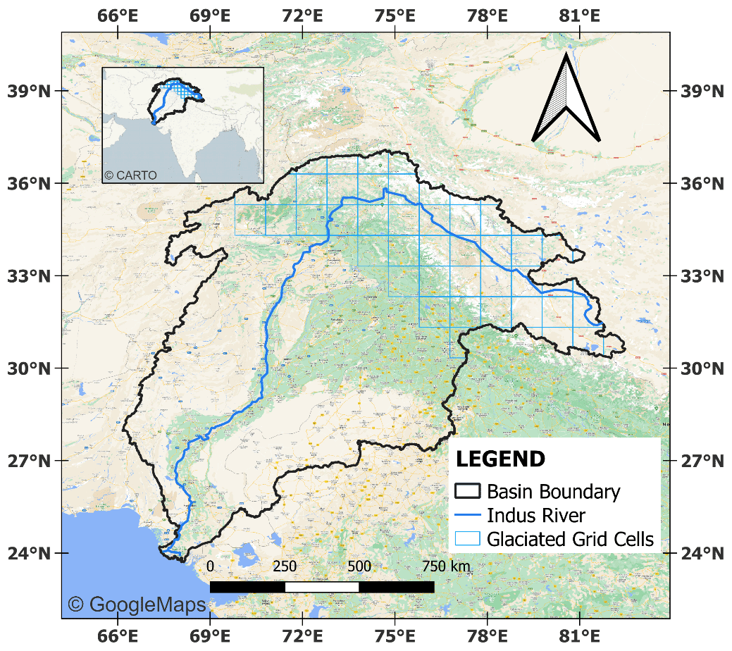
Figure 1 The Indus Basin. The blue squares represent the glaciated areas as cells of 1^∘ size. Basin boundaries by the International Centre for Integrated Mountain Development (ICIMOD). Main background map © Google Maps and inset map © Carto.

2 Materials and methods

2.1 Study area

The Indus River basin, shown in Fig. 1 (basin boundaries by ICIMOD, 2021), covers an area of 1.14 million km². The basin spans over four nations, India, Afghanistan, Pakistan, and China, and supports over 215 million people with an approximate water availability of 1329 m³ per head (Frenken, 2012). The Indus River is a perennial river originating from the Bokar Chu glacier in Mt. Kailash in Tibet. It flows through the Ladakh region in Kashmir, fed by the glaciers of the Himalayas, Karakoram, and the Hindu Kush ranges, entering the plains of Punjab in Kalabagh, Pakistan. In its journey, it is joined by the Kabul River from the west and Panjnad (Jhelum, Ravi, Chenab, Sutlej, and Beas) from the east to drain into the Arabian Sea. Almost 50 % of its discharge is due to snowmelt (Shrestha et al., 2019). Due to the complex terrain conditions, this basin is a data-scarce basin which makes monitoring of hydrological variables sparse and inconsistent. Being a transboundary basin, cooperation between nations also aggravates this situation. Hence, given that the TWSC estimates from GRACE are the only source for the entire Indus Basin, their uncertainty due to leakage and possible correction approaches must be studied thoroughly.

The winter climate over the Indus Basin is dominated by western disturbances embedded with the Indian winter monsoon. During the summer, the Indian monsoon (ISM) brings precipitation to the southern parts of the basin (Dimri et al., 2019). The mean annual rainfall varies between 90 and 500 mm in the downstream and midstream segments, while there is more than 1000 mm in the upstream catchments. The climate in the Indus Basin varies from subtropical arid and semi-arid to temperate sub-humid in Sindh and Punjab, to alpine in the mountainous highlands in the north, with average temperatures ranging between 2 and 49 ^∘C (Dimri et al., 2019). The hydro-climatic parameters in the upper Indus Basin are primarily influenced by glacier melt and in the lower part by human intervention in the form of different irrigation schemes and extensive groundwater depletion (Rodell et al., 2009).

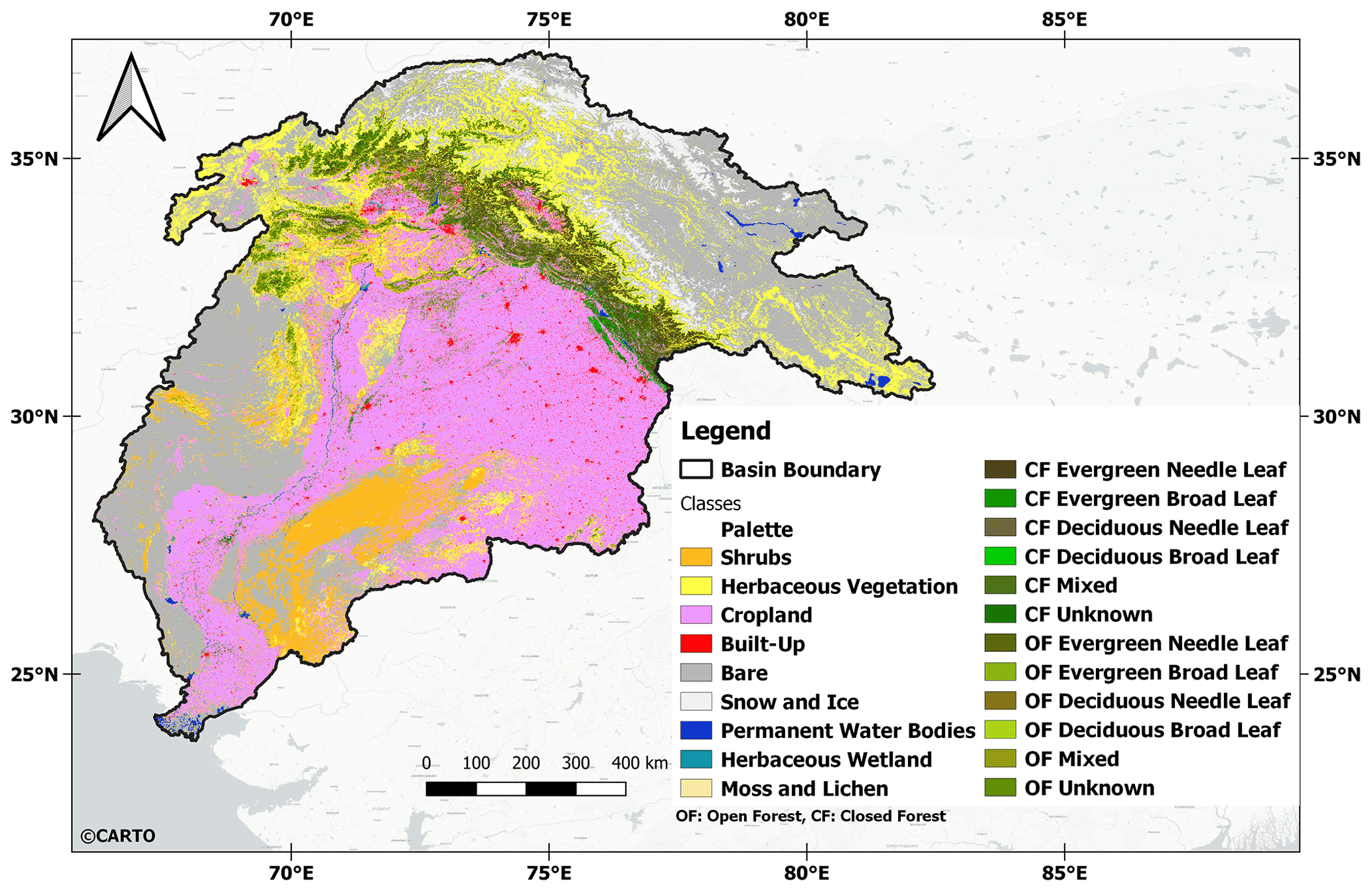
Figure 2 The land use land cover map (100 m resolution) of the Indus Basin for 2016, obtained from the Copernicus Global Land Cover Service. Background map © CARTO.

Hence, a complex hydrological regime exists in the entirety of the Indus Basin due to rapidly varying climatological and anthropogenic conditions across the basin. Figure 2, obtained from the Copernicus Global land cover service, shows the land cover distribution in the Indus Basin for 2016. Heavily irrigated areas lie along the river course and the central–east region of the basin (Cheema and Bastiaanssen, 2010). Due to the reduction in precipitation and increase in demand, groundwater has been the primary source of irrigation. The groundwater depletion in Punjab and the national capital region (just outside the Indus Basin boundaries) is a serious problem leading to severe localized land deformations (Garg et al., 2022). Due to rising mean annual temperatures, the evapo-transpiration (ET) is also high in these regions. Hence, human intervention is the dominant short-scale driver of TWS changes in these regions, as opposed to the upper Indus Basin, where glaciers and snowmelt dominate the TWS changes.

2.2 Datasets

2.2.1 GRACE data

The GRACE Level 2 data consisting of monthly Stokes coefficients of Earth's geopotential was used to derive estimates of TWSC over the Indus Basin. The data from three Science Data Centers, Jet Propulsion Laboratory (JPL), University of Texas, Center for Science and Research (CSR), and GeoForschungsZentrum (GFZ) in release 6 (RL06) were utilized up to degree 90. Only the months common to all three solutions and WGHM output were used. This resulted in 147 monthly solutions from April 2002 to December 2016. The GSM (denoted as is) products were used, containing fully normalized geopotential coefficients representing the full magnitude of land hydrology, ice, and solid Earth processes. In addition, the RL06 MASCON product from CSR was also utilized to compare the overall results of level 2 processing. The ICE-6G_D model was used to account for glacial isostatic adjustment (Peltier et al., 2018). This model is available up to degree and order 256 and provides secular rate of change of gravity field in mm yr⁻¹. The degree 1 coefficients from (Sun et al., 2016), distributed as Technical Note (TN-13) on the Tellus website, were used. The replacement C₂₀ coefficients from (Cheng and Ries, 2017), distributed as TN-11 on the Tellus website, were used. To derive GRACE-like errors for the design of simulation experiments, the monthly normal equations provided by TU Graz for the ITSG-2018 solutions (Kvas et al., 2019) in SINEX format were used.

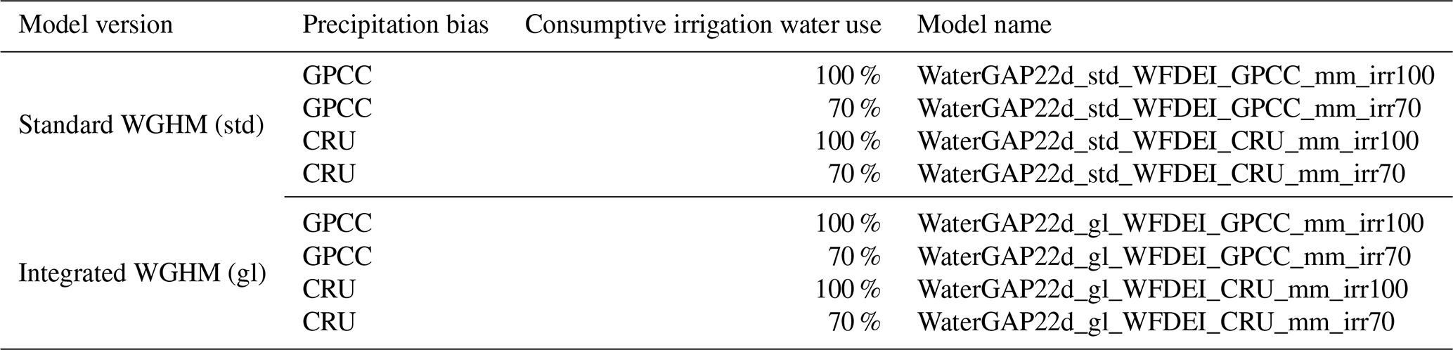
Table 1 Summary of WGHM 2.2d versions used in this study. The integrated WGHM version is standard WGHM with an additional glacier module from GGM. An average of four variants in each version were used in the study.

2.2.2 Model data

TWS anomalies from WGHM 2.2d, both standard and integrated versions, were used (Döll et al., 2003; Müller Schmied et al., 2016; Cáceres et al., 2020). The integrated version simulates glacier mass changes, unlike the standard version. Grids of 0.5^∘ resolution from April 2002 to December 2016 were used and resampled to 1^∘. For each version, there were four variants available with two climate forcings; ERA-Interim reanalysis (WFDEI) applied with WATCH Forcing Data (WFD) methodology and bias-corrected using precipitation data sets derived from rain gauge observations of either GPCC v5/v6 (Global Precipitation Climatology Centre; Schneider et al., 2015) or CRU TS3.10/TS3.21 (Climate Research Unit; Harris et al., 2014) and two irrigation variants; irrigation water use at 70 % of consumptive use (CU) and optimal CU. No single irrigation scenario can be assigned for the Indus Basin due to the heterogeneity in irrigation patterns. Hence, an average of these four variants was taken under each version (standard and integrated) to obtain the respective grids. Table 1 summarizes the variants of the model used in this study.

WGHM simulates water flows at a daily timescale on a 0.5^∘ by 0.5^∘ global grid, excluding Antarctica. Human intervention and its effect on water flows are also considered by simulating human water use in five sectors: irrigation, manufacturing, livestock farming, domestic use, and thermal power plants. The model requires daily meteorologic inputs of near-surface air temperature, precipitation (rainfall and snow), downward shortwave radiation, and downward longwave radiation. Reservoir data come from the Global Reservoir and Dam (GRanD) database, which includes 6862 reservoirs with a total storage capacity of 6197 km³ (Lehner et al., 2011).

Water balance is carried among three water storage compartments in the vertical direction: canopy, snow, and soil water storage. WaterGAP represents soil as a one-layer soil water storage compartment characterized by a land cover and soil-specific maximum storage capacity and soil texture. The groundwater is recharged from the soil, and storage is simulated after accounting for net abstractions from groundwater due to human use. A fraction of groundwater recharge is assumed to flow back to surface water bodies, and groundwater recharge under surface water bodies is neglected. The surface water storage comprises five sub-compartments: local lakes, local wetlands, global lakes, reservoirs, and global wetlands. At each stage, the storage is simulated by accounting for ET losses and net abstractions from lakes and reservoirs. Finally, the output from surface water bodies and groundwater flows into rivers, where the river water storage is simulated after accounting for the streamflow.

Groundwater surface water use (GWSUSE) model accounts for net abstractions from surface water and groundwater. Irrigation is assumed to vary with countries (efficiency of irrigation water use) and source of irrigation water. In groundwater-depleted areas, the CU from irrigation is considered 70 % of the optimal CU since farmers have less availability to satisfy the optimal requirements. In all other areas, it is assumed to be optimal. Country-specific efficiency values are used for surface water irrigation, while in case of groundwater irrigation, water use efficiency is set to a relatively high value of 0.7 worldwide. These abstractions are accounted for in the water balance for each compartment as described above.

The glacier mass changes not included in the WGHM are obtained from global glacier model (GGM) (Marzeion et al., 2012). GGM consists of a surface mass balance model based on the temperature index approach and model that accounts for changes in glacier geometry in feedback to compute the changes in glacier mass. The model is forced by a mean ensemble of seven atmospheric datasets, reducing the uncertainty inherent in the individual forcing datasets. As an initial condition for glacier geometry, data like glacier areas and boundaries are taken from Randolph Glacier Inventory (RGI v6) (Pfeffer et al., 2014). The model is calibrated using observed surface mass balance from World Glacier Monitoring Service (WGMS).

2.3 Methods

2.3.1 GRACE data processing

The GRACE level 2 SH coefficients from the GSM product represent the geopotential of Earth containing the full magnitude of land hydrology, ice, and solid Earth processes during each month t as in Eq. (1),

$$\begin{array}{}\text{(1)}& \begin{array}{rl}V\left(r,\mathit{\theta },\mathit{\lambda },t\right)& ={\displaystyle \frac{\mathrm{GM}}{R_{\mathrm{e}}}}\sum _{n=\mathrm{0}}^N{\left({\displaystyle \frac{R_{\mathrm{e}}}{r}}\right)}^{n+\mathrm{1}}\sum _{m=\mathrm{0}}^n{P}_n^m\left(\cos \mathit{\theta }\right)\\ & \left\{C_{nm}^t\cos m\mathit{\lambda }+S_{nm}^t\sin m\mathit{\lambda }\right\},\end{array}\end{array}$$

where θλ are co-latitude and longitude respectively, n,m are degree and order of the expansion, N is the maximum degree used which was 90 in this case, $P_n^m$ are the associated Legendre's functions, $C_{nm}^t$ and $S_{nm}^t$ are the spherical harmonic coefficients at month t, and R_e (6378 km) is Earth's equatorial radius.

The mean static gravity field is removed to obtain gravity field anomalies. In this study, the mean period was taken as the mean of the entire study period. Monthly solutions common to all three (JPL, CSR, and GFZ) centers till December 2016 were extracted with a tolerance of 15 d in the middle of each monthly solution epoch. Running means over three consecutive solutions are taken, which reduces the noise in the solutions. Glacial isostatic adjustment (GIA) is the ongoing secular response of Earth's surface to the mass changes that occurred due to the deglaciation process on Earth and is removed using the ICE-6G model (Peltier et al., 2018). The same GIA model used in CSR MASCONS is used to maintain consistency. Assuming mass changes occur in a thin spherical shell (∼ 15 km) around Earth (Wahr et al., 1998), these coefficients are multiplied by degree-dependent factors to obtain surface mass changes coefficients in terms of equivalent water height (EWH). The resulting change in surface mass density is obtained as Eq. (2),

$$\begin{array}{}\text{(2)}& \begin{array}{rl}\mathrm{\Delta }\mathit{\sigma }\left(\mathit{\theta }\mathit{\lambda }t\right)& ={\displaystyle \frac{R_{\mathrm{e}}{\mathit{\rho }}_{\mathrm{avg}}}{\mathrm{3}}}\sum _{n=\mathrm{0}}^N\left({\displaystyle \frac{\mathrm{2}n+\mathrm{1}}{\mathrm{1}+k_n^{\prime }}}\right)\sum _{m=\mathrm{0}}^n{P}_n^m\left(\cos \mathit{\theta }\right)\\ & \left\{\mathrm{\Delta }{C}_{nm}^t\cos m\mathit{\lambda }+\mathrm{\Delta }{S}_{nm}^t\sin m\mathit{\lambda }\right\},\end{array}\end{array}$$

where ρ_avg is the average density of Earth (5515 kg m⁻³) and $k_n^{\prime }$ are the elastic load Love numbers of Earth.

Swenson filter (Swenson and Wahr, 2006) is used for destriping, which removes the correlated errors in even and odd degrees. The filter parameters are chosen after Sasgen et al. (2018), which minimizes the signal and noise contamination between mid-latitude and polar regions during destriping. A Gaussian low pass filter of half width 300 km is employed to reduce the random errors in higher degree terms. Grids of filtered surface mass changes are obtained as Eq. (3),

$$\begin{array}{}\text{(3)}& \begin{array}{rl}\mathrm{\Delta }\mathit{\sigma }\left(\mathit{\theta }\mathit{\lambda }t\right)& ={\displaystyle \frac{R_{\mathrm{e}}{\mathit{\rho }}_{\mathrm{avg}}}{\mathrm{3}}}\sum _{n=\mathrm{0}}^N\left({\displaystyle \frac{\mathrm{2}n+\mathrm{1}}{\mathrm{1}+k_n^{\prime }}}\right)\sum _{m=\mathrm{0}}^n{P}_n^m\left(\cos \mathit{\theta }\right)W_n\\ & \left\{\mathrm{\Delta }{C}_{nm}^t\cos m\mathit{\lambda }+\mathrm{\Delta }{S}_{nm}^t\sin m\mathit{\lambda }\right\},\end{array}\end{array}$$

where W_n are degree-dependent factors of Gaussian filter in spectral-domain (Sasgen et al., 2018).

From the filtered GRACE surface density coefficients, mass changes for the Indus Basin are obtained by regional integration using the region function defined in Eq. (4),

$$\begin{array}{}\text{(4)}& \mathrm{RF}\left(\mathit{\theta }\mathit{\lambda }\right)=\left\{\begin{array}{c}\mathrm{1}\\ \mathrm{0}\end{array}\right\}\begin{array}{ccc}\forall (\mathit{\theta },\mathit{\lambda })& \in & R\\ \forall (\mathit{\theta },\mathit{\lambda })& \in & \mathrm{\Omega }-R\end{array},\end{array}$$

where RF is the region function inside the region R of the Indus Basin and region Ω is the total surface area of Earth. This region function is transformed to spectral-domain (up to degree 90), and the corresponding coefficients are multiplied with filtered surface density coefficients to obtain mass changes for the Indus Basin, ΔM, as in Eq. (5),

$$\begin{array}{}\text{(5)}& \begin{array}{rl}\mathrm{\Delta }M\left(\mathit{\theta }\mathit{\lambda }t\right)& ={\displaystyle \frac{R_{\mathrm{e}}{\mathit{\rho }}_{\mathrm{avg}}}{\mathrm{3}}}\sum _{n=\mathrm{0}}^N\left({\displaystyle \frac{\mathrm{2}n+\mathrm{1}}{\mathrm{1}+k_n^{\prime }}}\right)\sum _{m=\mathrm{0}}^{\mathrm{n}}{P}_n^m\left(\cos \mathit{\theta }\right)W_n\\ & \left\{R_{nm}^{\mathrm{c}}\mathrm{\Delta }{C}_{nm}^t\cos m\mathit{\lambda }+R_{nm}^{\mathrm{s}}\mathrm{\Delta }{S}_{nm}^t\sin m\mathit{\lambda }\right\},\end{array}\end{array}$$

where R_c and R_s are respectively the cosine and sine coefficients of the region function in the spectral domain.

2.3.2 Scaling factors determination

WGHM anomalies were centered around the mean of the entire observation period (April 2002–December 2016) by including only GRACE months. Unfiltered mass change time series for the Indus Basin from both versions were obtained using the region function in Eq. (4), by integrating the global grids over the surface of Earth as in Eq. (6),

$$\begin{array}{}\text{(6)}& \mathrm{\Delta }{M}_{\mathrm{region}}\left(t\right)=\int \mathrm{\Delta }\mathit{\sigma }\left(\mathit{\theta },\mathit{\lambda },t\right)\mathrm{RF}\left(\mathit{\theta },\mathit{\lambda }\right)\mathrm{d}\mathrm{\Omega },\end{array}$$

where $\mathrm{d}\mathrm{\Omega }=R_{\mathrm{e}}^{\mathrm{2}}\sin \mathit{\theta }\mathrm{d}\mathit{\theta }\mathrm{d}\mathit{\lambda }$ is an element of the area on the region surface. The global grids are then transformed to the spherical harmonic domain up to degree 90 and applied with Swenson destriping and Gaussian low pass filter in the same manner as described in Sect. 2.3.1. The filtered coefficients are transformed back to the spatial domain to obtain filtered model grids. Regional integration in the spectral domain is performed with filtered model coefficients to get filtered model mass change time series.

A single scaling factor (k) for the entire basin is derived by a least squares regression between unfiltered model time series and filtered model time series, that is, by minimizing L in Eq. (7),

$$\begin{array}{}\text{(7)}& L=\sum _{t=\mathrm{1}}^T{\left(\mathrm{\Delta }{S}_t^{\mathrm{u}}-k\mathrm{\Delta }{S}_t^{\mathrm{f}}\right)}^{\mathrm{2}},\end{array}$$

over the entire period of study. In Eq. (7), $\mathrm{\Delta }{S}_t^{\mathrm{u}}$ is the unfiltered and $\mathrm{\Delta }{S}_t^{\mathrm{f}}$ is the filtered model mass for the tth month. A scaling factor for each grid cell in a 1⁰×1⁰ grid is derived using the unfiltered model grid and filtered model grid and minimizing L in Eq. (7) but at every grid cell in the basin. This is done for both versions of WGHM to obtain a 1^∘ resolution map of scaling factors.

To derive frequency-dependent scaling factors, the total mass changes from unfiltered and filtered model versions are decomposed into long-term linear, seasonal, and residual components as Eq. (8),

$$\begin{array}{}\text{(8)}& \mathrm{\Delta }S=\mathrm{\Delta }{S}_{\mathrm{long}\mathrm{term}}+\mathrm{\Delta }{S}_{\mathrm{sesonal}}+\mathrm{\Delta }{S}_{\mathrm{residual}}.\end{array}$$

For this purpose, a time series model is fit to the data using least squares as in Eq. (9),

$$\begin{array}{}\text{(9)}& \begin{array}{rl}{y}_i& ={\mathit{\beta }}_{\mathrm{0}}+{\mathit{\beta }}_{\mathrm{1}}\left(\mathrm{t}\right)+{\sum }_{k=\mathrm{1}}^n\\ & \left[{\mathit{\beta }}_k^{\mathrm{c}}\cos \left({\displaystyle \frac{\mathrm{2}\mathit{\pi }}{T_k}}t\right)+{\mathit{\beta }}_k^{\mathrm{s}}\sin \left({\displaystyle \frac{\mathrm{2}\mathit{\pi }}{T_k}}t\right)\right]+\mathit{\nu }\left(t\right),\end{array}\end{array}$$

where β₁ is the linear trend, ${\mathit{\beta }}_k^{\mathrm{c}}$ and ${\mathit{\beta }}_k^{\mathrm{s}}$ are the amplitudes of the cosine and sine terms of the periodic component with a period T_k, and t represents the month with respect to the mean of the observation period. However, the periods (T_k) of the seasonal terms are unknown. For this study, the unknown periods are found from the data itself using a Lomb–Scargle (LS) periodogram analysis (Scargle, 1982) which allows detection of weak periodic signals in otherwise random, unevenly sampled data.

From this analysis, the peaks were found at annual and semi-annual periods. The false alarm probabilities associated with each peak were minimal ($\sim {\mathrm{10}}^{-\mathrm{5}}$), which shows that these periods are significant. These periods were used in Eq. (9) for time series decomposition. The trend, annual, and semi-annual components are separated in both model versions' unfiltered and filtered time series. Then a least squares fit is carried out for all three components separately to obtain three scaling factors that minimize the expression in Eq. (10),

$$\begin{array}{}\text{(10)}& \begin{array}{rl}L& =\sum _{j=\mathrm{1}}^N\left(\mathrm{\Delta }{S}_j^{\mathrm{u}}-k_j\mathrm{\Delta }{S}_j^{\mathrm{f}}\right),\\ & \text{ where }j=\left\{\begin{array}{c}\text{ trend }\\ \text{ annual }\\ \text{ semi-annual }\end{array}\right\},\end{array}\end{array}$$

where k_j is the scaling factor for jth component.

Figure 3 The schematic diagram for deriving and applying the three scaling schemes.

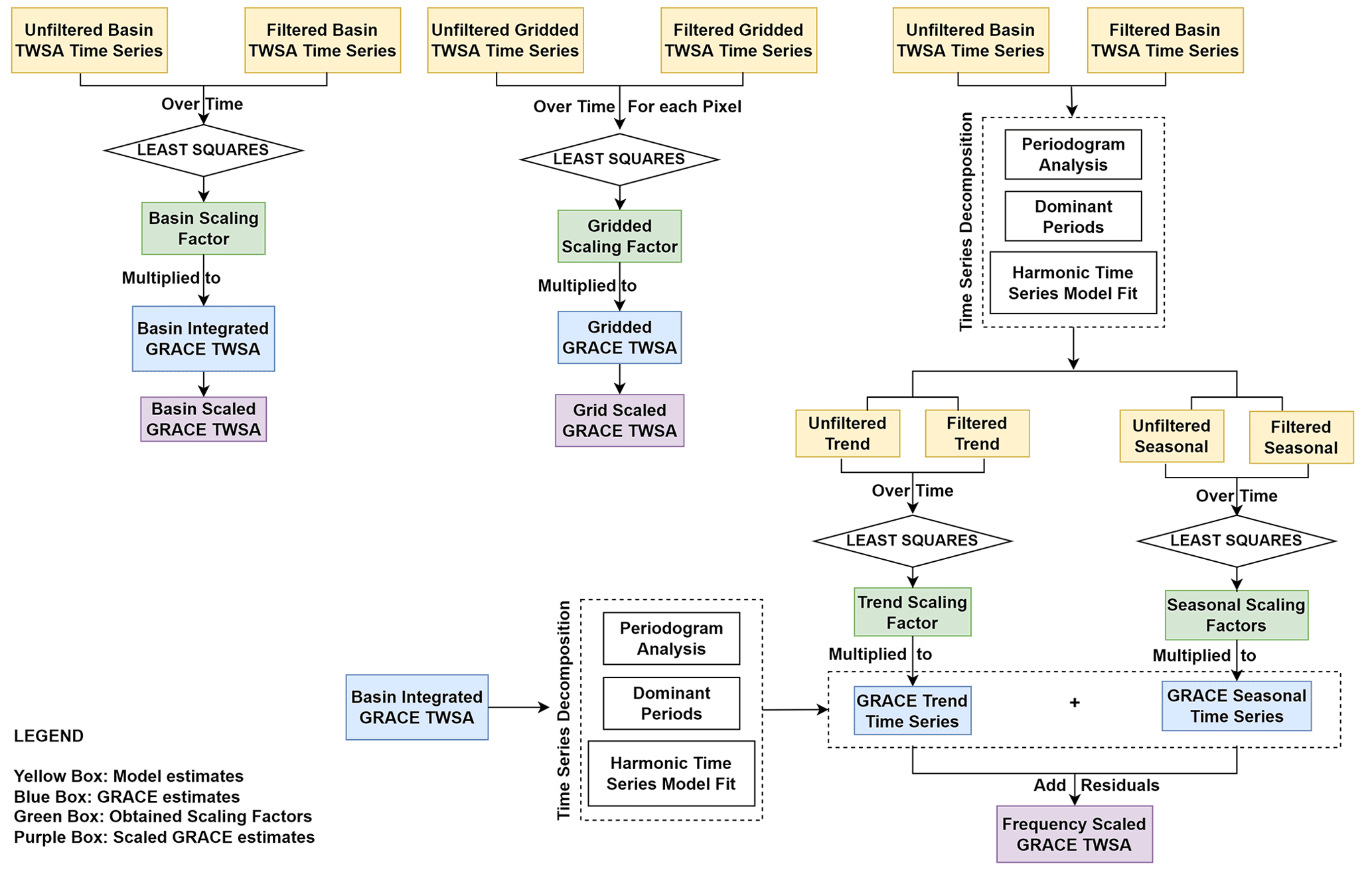
Figure 3 presents the schematic of deriving scaling factors (in green boxes) from filtered and unfiltered model time series (in yellow boxes) and applying them to corresponding GRACE time series (in blue boxes) to obtain scaled GRACE estimates (in purple boxes).

2.3.3 Implementation of data-driven correction approach

The DDC approach or the method of deviation (Vishwakarma et al., 2017) uses twice-filtered GRACE fields to determine two correction terms for the regional averages of filtered GRACE fields, namely the leakage and deviation integrals for the entire basin. We used the method codes provided by the authors (and through personal communication with the lead author) to compute basin-averaged DDC corrected time series for the Indus Basin to compare with our scaled basin averaged time series.

2.3.4 Design of simulation experiment

Due to the unavailability of distributed in situ data, we designed a simulation experiment using WGHM and monthly GRACE TWS errors to assess the extent to which the scaling schemes can recover the signal lost to filtering. We use WGHM fields as a proxy for true TWS signals and corrupt them with GRACE-like errors (Willen et al., 2022). For this, we first derived the error covariance matrices from the normal equations provided by TU Graz for the ITSG solutions (Kvas et al., 2019) from degree 2 onwards. For the degree 1 coefficients, the corresponding error covariances were computed from an ensemble of 12 different estimates derived following Swenson et al. (2008), arising from four GRACE products (JPL, CSR, and GFZ release 6, ITSG-2018) and three GIA models (A et al., 2013; Caron et al., 2018; Peltier et al., 2018). Assuming the errors to follow multivariate random distribution, we derived their random realizations in the SH domain from the covariance matrices using Cholesky decomposition. We then added these errors to the WGHM fields in SH domain and filtered using the same filter used in the study for GRACE (Swenson destriping +300 km Gaussian). These filtered–corrupted WGHM fields now represent GRACE-like observations. Finally, using the scaling factors derived in the study, we rescaled these filtered–corrupted WGHM fields as per the respective schemes (Fig. 3) to recover the lost signals as rescaled WGHM fields.

We use GRACE errors from the ITSG solutions for assessing scaled estimates of GRACE solutions in our study since the normal equations from three centers – JPL, CSR, and GFZ – are not publicly available. Moreover, using ITSG-based errors can be justified by the following: our study uses a monthly running average of the three solutions, which means the errors are already reduced. The ITSG solution which has been shown to have less noise than the JPL, CSR, and GFZ solutions (Ditmar, 2022) thus provides a reasonable estimate of the average error content.

2.3.5 Assessment of uncertainty components

Two quantities are computed using WGHM as a proxy to the true signal to assess the uncertainty specific to leakage and scaling. Equation (11) provides the initial leakage due to filtering, and Eq. (12) provides the amount of leakage not covered by the scaling factors, termed residual leakage.

$$\begin{array}{}\text{(11)}& {\displaystyle }\begin{array}{rl}\text{Initial Leakage Error}& =\text{std}\left(\mathrm{\Delta }{S}_t^{\mathrm{u}}-\mathrm{\Delta }{S}_t^{\mathrm{fc}}\right)\\ & \times {\displaystyle \frac{\mathrm{RMS}\left(\mathrm{\Delta }{G}_t\right)}{\mathrm{RMS}\left(\mathrm{\Delta }{S}_t^{\mathrm{f}}\right)}}\end{array}\text{(12)}& {\displaystyle }\begin{array}{rl}\text{Residual Leakage Error}& =\text{std}\left(\mathrm{\Delta }{S}_t^{\mathrm{u}}-k\mathrm{\Delta }{S}_t^{\mathrm{fc}}\right)\\ & \times {\displaystyle \frac{\mathrm{RMS}\left(\mathrm{\Delta }{G}_t\right)}{\mathrm{RMS}\left(\mathrm{\Delta }{S}_t^{\mathrm{f}}\right)}},\end{array}\end{array}$$

where std represents the standard deviation, RMS represents the root mean square of the time series indexed by t, k represents any one of the scaling factors schemes, ΔG_t represents GRACE mass time series, and $\mathrm{\Delta }{S}_t^{\mathrm{fc}}$ represents the filtered–corrupted model time series. If the scaling factors work, the residual leakage should be less than the initial leakage. This quantification assumes all the variation in the difference between filtered–corrupted and unfiltered model time series to represent leakage error (making no distinction between individual effects on underlying signal and noise). It is thus meaningful for intercomparison of different schemes but not as a true estimate of leakage error. This standard deviation is multiplied by the ratio of RMS of GRACE and filtered–corrupted model time series to account for the amplitude difference in GRACE and model (Landerer and Swenson, 2012).

The uncertainty estimation of GRACE mass estimates is done following Groh et al. (2019), which uses only the time series of derived GRACE masses to determine noise. The unscaled GRACE time series contains errors from measurement, leakage, GIA, and C₂₀. Since this approach provides the temporally uncorrelated component of total GRACE errors, the effect of scaling on the random component of time series (thus a random component of leakage) can be compared. The uncertainties from GIA models (<1 mm yr⁻¹ equivalent sea level) and C₂₀ (<0.1 mm yr⁻¹ equivalent sea level) coefficients are almost negligible for the Indus Basin and, hence, are not considered (Caron et al., 2018; Blazquez et al., 2018). A high pass filter is applied to the residuals of the GRACE time series (after removing trend and seasonal components) to remove the un-modeled inter-annual components in the residuals. The filter width is chosen to be 18 months (6 sigma width of Gaussian hat =18 months), which means all the signal with a larger than 18-month period is removed, leaving temporally uncorrelated errors referred to as noise. This noise contains the GRACE measurement error and the random component of the initial leakage error. A scaling factor generated from high pass filtering random white noise signals is multiplied to account for the damping of any white noise component during high pass filtering. Similarly, this process is repeated for scaled GRACE time series. The corresponding scaled noise contains the scaled measurement and residual random leakage errors.

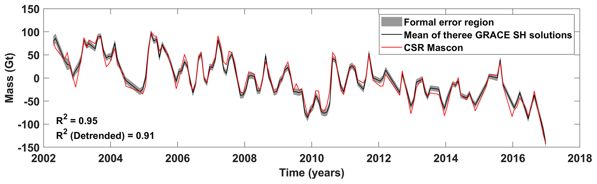
Figure 4 Time series of mass anomalies (mean removed: 2002–2016) in the Indus Basin derived from GRACE spherical harmonic solution (mean of JPL, CSR, and GFZ), corrected with ICE6G, and filtered with Swenson destriping and 300 km Gaussian filter.

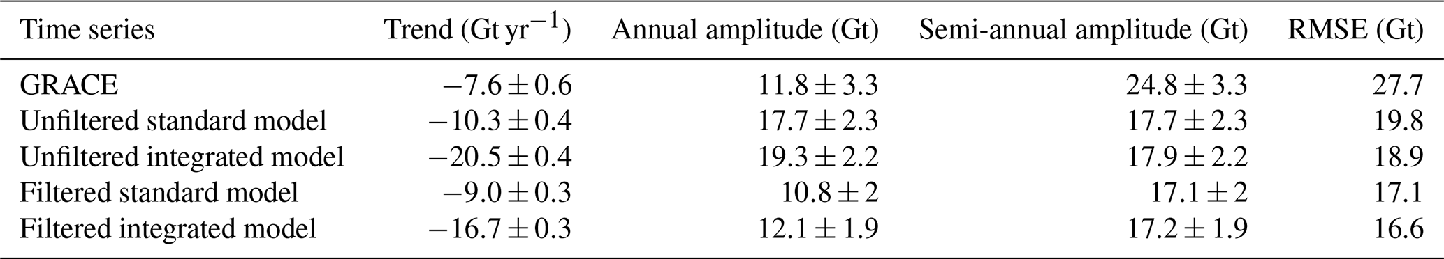
Table 2 Summary of parameters from time series fitting of basin averages.

3 Results and discussion

3.1 Mass change estimates from GRACE and WGHM

Figure 4 shows the result of the processing scheme followed to obtain mass change time series from the average of three GRACE level 2 SH solutions and MASCON time series from CSR. The shaded region depicts the 3σ interval of uncertainties from formal errors of the SH coefficients provided by the centers. These uncertainties are propagated to the mass estimates and averaged for three centers by the law of error propagation over Eq. (5) in Sect. 2.3.1. A GRACE trend value of $-\mathrm{7.6}\pm \mathrm{0.6}$ Gt yr⁻¹ is obtained (Table 2). Similar values of −8.6 Gt yr⁻¹ from (Scanlon et al., 2018) and −9.1 Gt yr⁻¹ from (Kvas et al., 2019) have been reported. The differences can be attributed to processing strategies and different data releases used in these studies. The performance of the processing scheme is assessed by comparison to the time series obtained from the Level 3 release 6 CSR MASCON (CSR-M) solution (Save et al., 2016). Although derived from the same level 1 data as SH solutions, MASCONS are constrained to reduce the leakage effect arising from the post-processing step. Figure 4 also shows the GRACE SH and CSR-M time-series correlation for the Indus Basin. The high value of Pearson's correlation coefficient (R²=0.95) indicates that the SH solution and processing strategy used are nearly as good as the MASCON solution for the Indus Basin. An R² value of 0.91 is obtained when both time series are de-trended, which confirms that the high values are not a spurious result.

Figure 5 Basin-averaged time series from GRACE SH, standard WGHM, and integrated WGHM for the Indus Basin.

Figure 5 shows the mass anomaly time series from the standard and integrated version of WGHM along with the GRACE SH-based time series. A significantly more negative trend is seen in the integrated version ($-\mathrm{20.5}\pm \mathrm{0.4}$ Gt yr⁻¹) than in the standard version ($-\mathrm{10.3}\pm \mathrm{0.4}$ Gt yr⁻¹), indicative of significant glacier melt in the Indus Basin, which has a dominating effect on the overall TWS trend of the Indus Basin. The negative trend from the standard version can be attributed to the human-induced changes due to severe groundwater depletion for meeting the irrigation demands in the Indus plains (Rodell et al., 2009) and increasing losses from ET due to climate-induced changes from increasing mean annual temperatures (Shrestha et al., 2019).

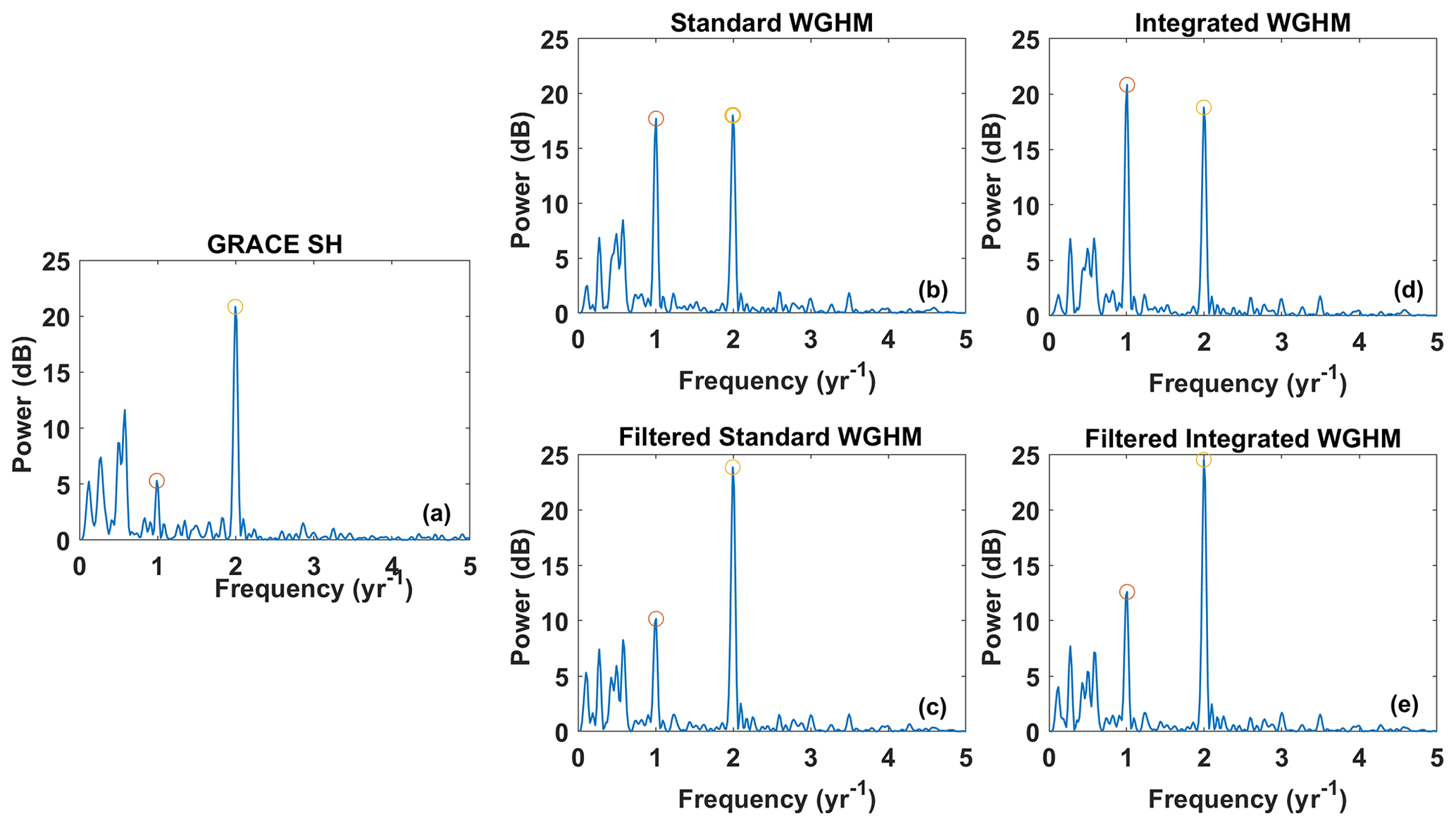
Figure 6 Lomb–Scargle periodograms for basin-averaged time series from (a) GRACE SH, (b) unfiltered standard WGHM, (c) unfiltered integrated WGHM, (d) filtered standard WGHM, and (e) filtered integrated WGHM. The peaks marked were selected as dominant for time series fit.

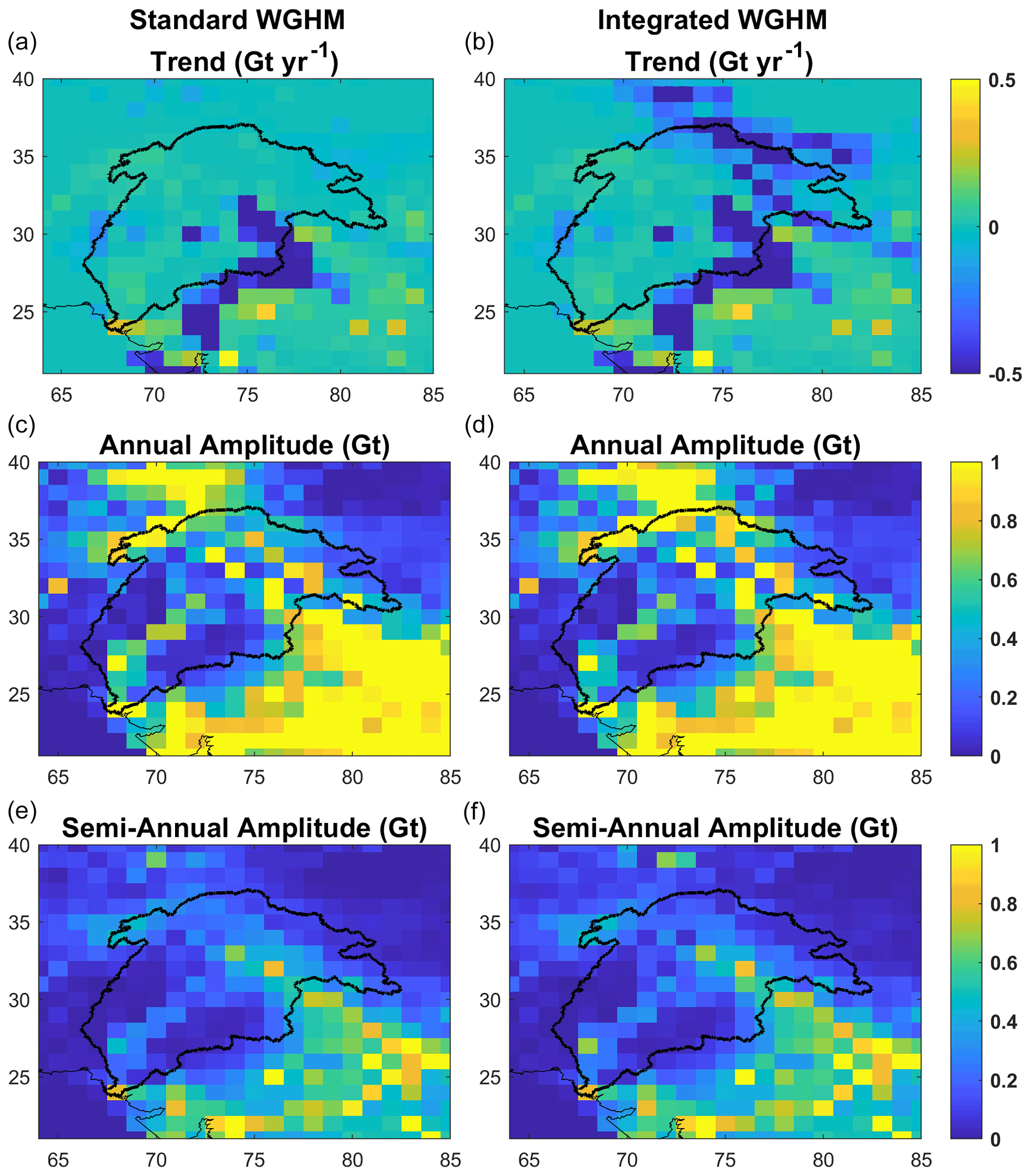
Figure 7 Spatial patterns of trend, annual, and semi-annual mass changes from WGHM standard (left) and integrated (right) versions.

The periodogram analysis of the standard and integrated version (Fig. 6b, c) shows clear peaks at annual and semi-annual frequencies. The peak frequencies obtained from the model and GRACE (Fig. 6a) are almost identical, confirming the ability of GRACE to observe small seasonal signals in the Indus Basin, which is mainly dominated by trends. However, from a subsequent time-series fit (Table 2), the annual amplitude (11.8±3 Gt) obtained from GRACE is much smaller than the semi-annual amplitude (24.8±2.9 Gt). It is found to be the artifact of filtering, as explained later in Sect. 3.2. Figure 7 shows the spatial distribution of different components of mass changes from WGHM standard and integrated versions. Close to the northern basin boundary, the annual signal content is higher in the integrated version than in the standard version, while the semi-annual component is almost the same. This is due to the annual component of glacier mass change contribution absent in the standard version. Respective amplitudes from the model time series fit (Table 2) also reflect this. The semi-annual seasonality in TWS changes results from bimodal precipitation distribution in the Indus Basin. The inter-annual signal content (area of the frequency spectrum in the inter-annual bandwidth) is almost identical in both model versions and GRACE. This shows that adding glacier mass changes to WGHM does not contribute to the inter-annual variations. These inter-annual variations are probably the result of long-term groundwater depletion (Pradhan, 2014) and inter-annual variability resulting from winter/spring precipitation over the upper Indus Basin due to El Niño–Southern Oscillation (ENSO) (Krakauer, 2019).

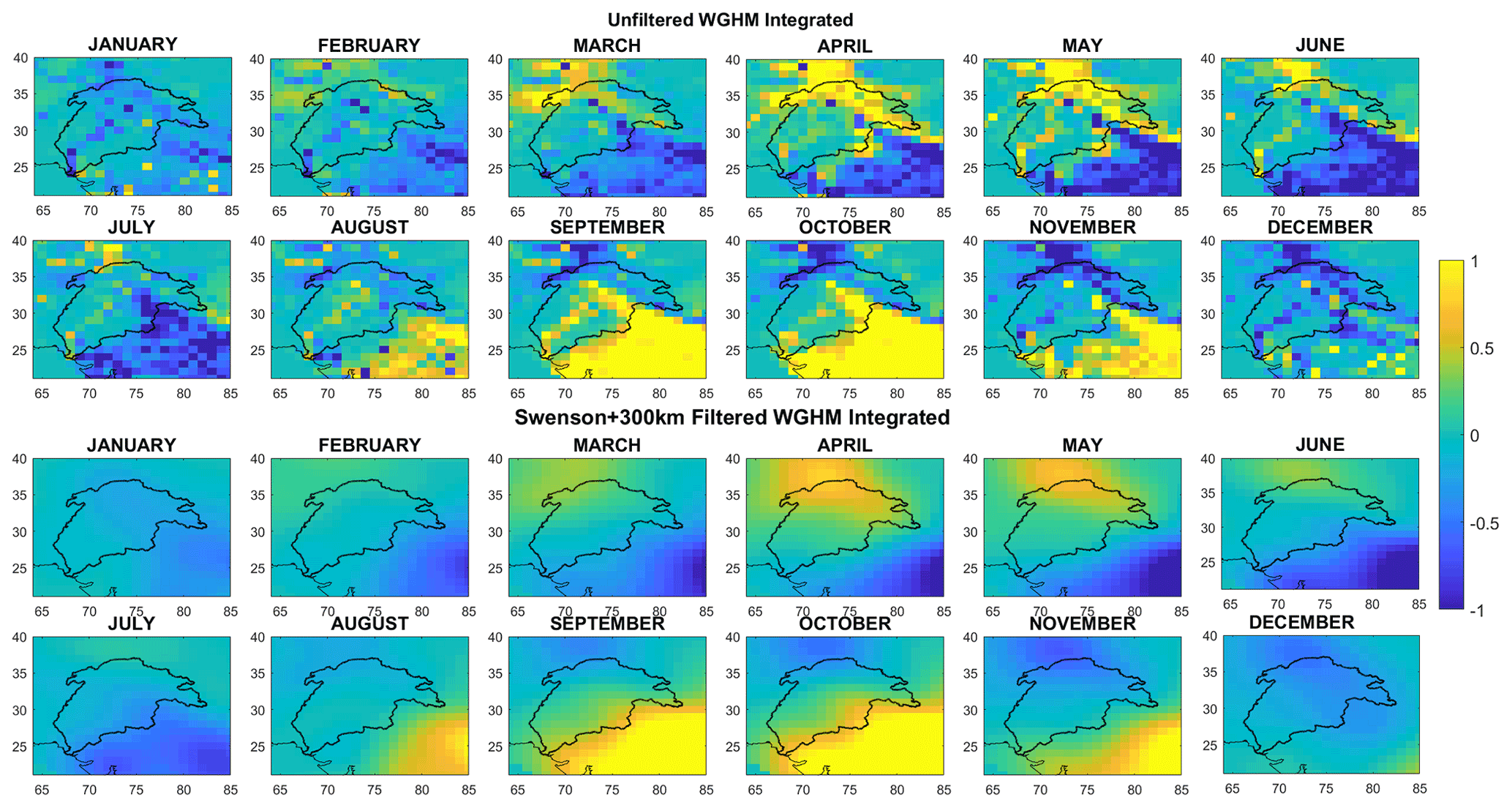
Figure 8 Mean mass anomalies (in Gt) for each month from April 2002–December 2016 obtained from WGHM Integrated: unfiltered (top) and filtered (bottom). Refer to Fig. 2 for land cover information.

3.2 Effect of filtering

Spatially, the effect of filtering is visualized in Fig. 8, which shows mean TWS anomalies for each calendar month from the unfiltered and filtered WGHM Integrated version. Local features and small-scale changes in TWS are smoothed out and reduced in amplitude. Large-scale changes in TWS (right panel, Fig. 8) follow the pattern of bimodal precipitation distribution in the Indus Basin due to western disturbances and ISM (Hasson et al., 2016; Hussain et al., 2020). The northwest to southeast increase in storage (reduction of blue color intensity) during the winter months (December to February) and pre-monsoon months (March to May) can be attributed to western disturbances. It is worth mentioning that there is generally a 1-month lag between precipitation and storage in this region. The southeast to the northwest increase of storage (decrease in blue and increase of yellow intensity) during the summer from July to October can be attributed to ISM. October and November show the retreat of monsoon and hence decreasing storage. Small-scale TWS changes (left panel, Fig. 8) are driven by heavy irrigation along the river, southeast Indus plains, and snow and glacier melt in the upper Indus Basin.

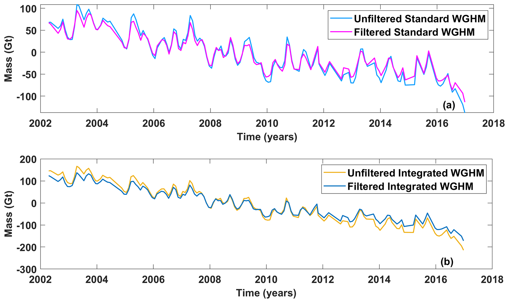
Figure 9 Unfiltered and filtered basin-averaged time series from (a) standard WGHM and (b) integrated WGHM version. Note the different y axis scales.

Temporally, the filtering dampens the trend, i.e., makes it less negative, in both the model versions (Fig. 9a, b). The dampening is by ∼ 13 % for the standard version and stronger, by ∼ 20 %, for the integrated version. The filtering brings the model-based trends closer to the GRACE-based trends, partly explaining the trend differences between filtered GRACE-based and unfiltered model-based time series.

The effect of filtering on seasonal signals can be analyzed from Fig. 6d, e. The peaks are obtained at the same frequencies as the unfiltered time series, which shows that filtering does not induce any additional periodicity of mass changes in the Indus Basin. From the relative peak heights of annual and semi-annual frequencies, it is also clear that filtering affects annual and semi-annual mass changes differently. The time series fit (Table 2) shows that filtering significantly reduces the annual amplitudes in both versions, while the semi-annual amplitudes are reduced only slightly. Hence, both versions show annual mass variations to leak out, explaining why the annual peak from GRACE (Fig. 6a) is suppressed. This is a significant effect of filtering and must be restored by scaling.

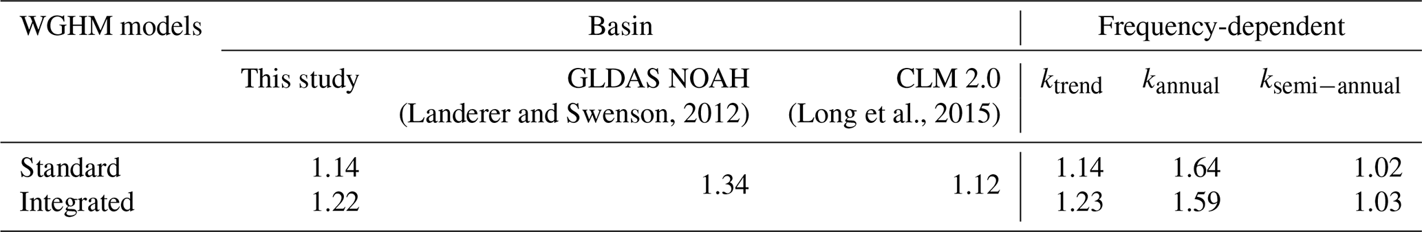
Table 3 Basin-scale factors and frequency-dependent scale factors for the Indus Basin. Basin-scale factors from two different studies are given for reference.

3.3 Scaling factors

3.3.1 Basin-scale factors

Basin scaling factors of k_s=1.14 from the standard version and k_g=1.22 from the integrated version are obtained. These values are greater than one, indicating that filtering causes the overall mass changes to leak out; hence, a factor greater than 1 is required to restore the signal. However, the values are small, indicating that the Indus Basin has a small leakage amount overall. Basin scale factors from two studies have reported similar values (Table 3). The addition of glacier mass changes in the model leads only to a minor effect on the basin-scale factor. Glacier mass changes are located at the edge of the basin and suffer from more leakage out. This explains the slightly larger scaling factor from the integrated version. The similarity of our results to results from other studies that used different models indicates that basin-scale factors are not very sensitive to the model used for the Indus Basin.

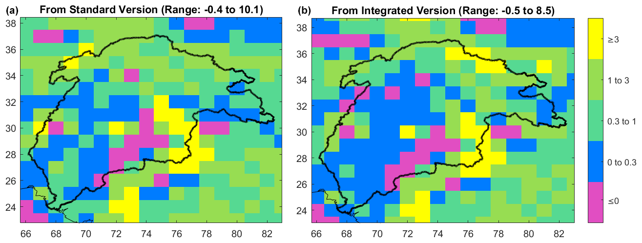
Figure 10 Gridded scaling factor map from the standard (a) and integrated (b) version of WGHM. The grid size is 1^∘ equiangular.

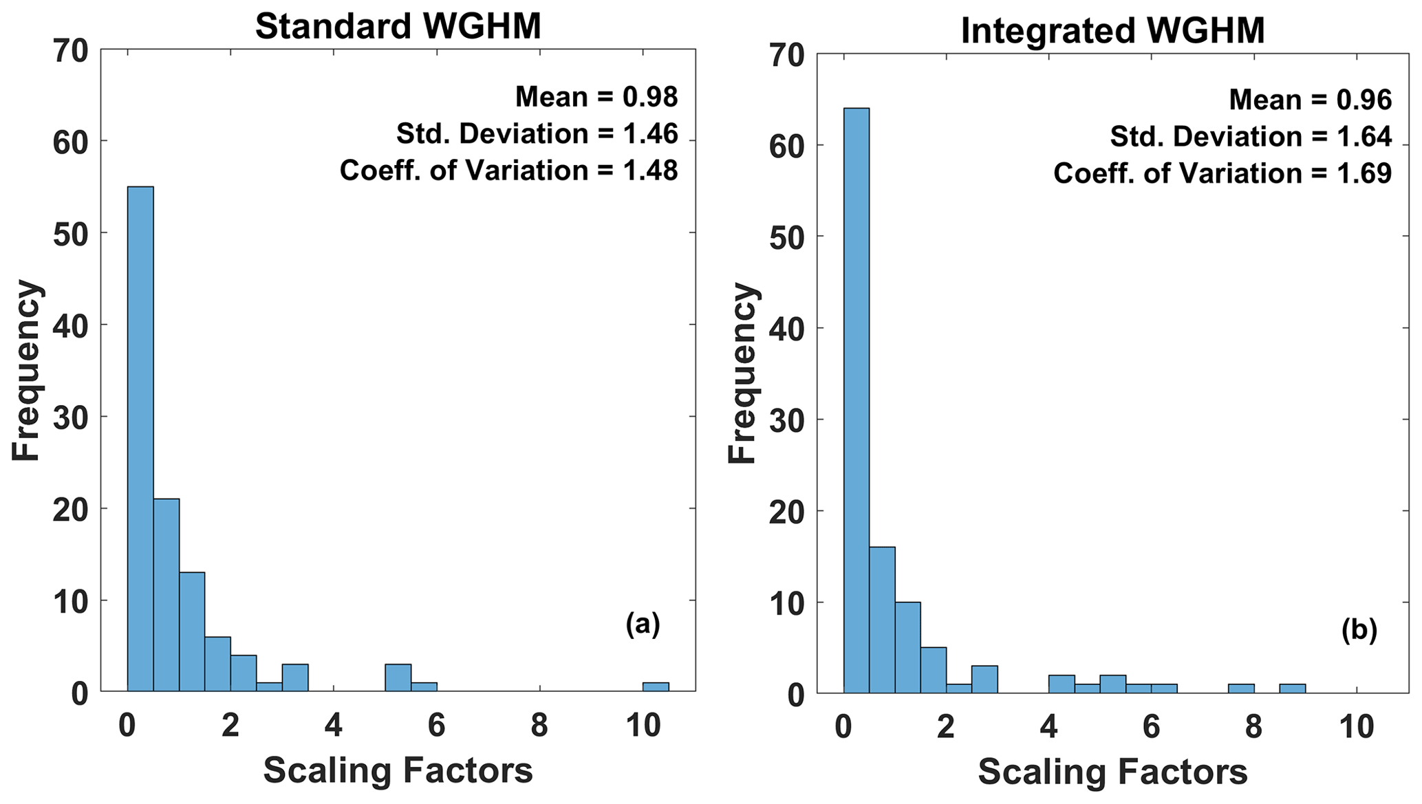
Figure 11 Frequency distributions of grid scaling factors from (a) standard and (b) integrated WGHM versions for the Indus Basin. The mean, standard deviation, and coefficient of variation (CV) are inset. Negative scaling factors are excluded.

Table 4 Interpretation of gridded scaling factors.

3.3.2 Gridded scaling factors

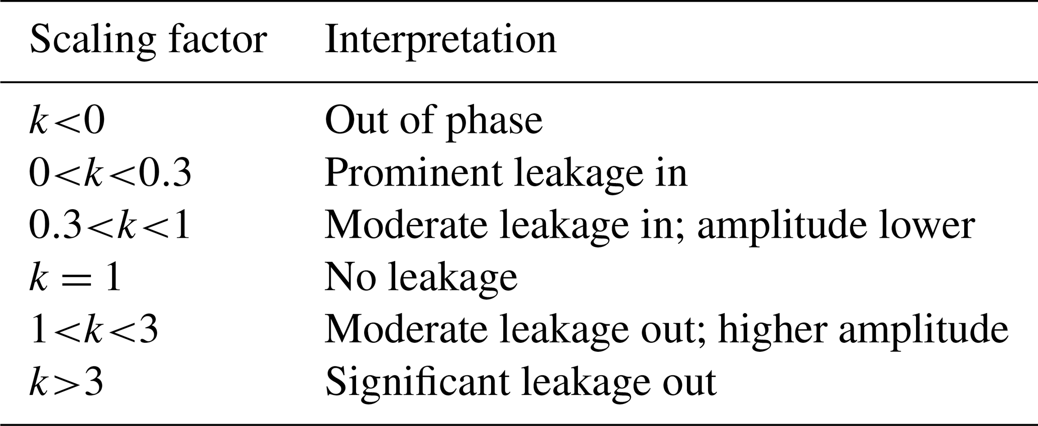
Figure 10 shows the gridded scaling factors in 1^∘ resolution maps from the standard (left) and the integrated version (right). The maps include 108 scaling factors, one for each pixel inside the Indus Basin. From the standard version, the scaling factors ranged from −0.4 to 10.1. From the integrated version, the scaling factors ranged from −0.5 to 8.5. Significant differences between the two occur in the upper Indus Basin, where the glaciers are located. Table 4 lists the standard interpretation of gridded scaling factor values used in most studies (Long et al., 2015). Figure 11 shows the histogram of scaling factors from both model versions.

From the standard version, scaling factors for 13 grid cells are negative. These grid cells were excluded for scaling, considering out-of-phase behavior with respect to their neighboring grid cells. Most scaling factors are less than 1 (67 grid cells), out of which most are less than 0.5 (55 grid cells), indicating that a large part of the basin suffers from moderate to significant leakage-in. These small scaling factors occur mainly in the lower reaches of the basin (Indus plains) and upper Indus Basin, where non-glacier mass changes are small in magnitude. Few grid cells stand out with larger scaling factors (>3), which depict large local mass changes in the pixel. These occur in the southeast Indus Basin region, which has a larger magnitude of TWS changes due to ISM and human intervention in the form of irrigation and groundwater depletion. These more considerable changes leak out to nearby dry regions of the upper Indus Basin (as represented in the standard version), requiring greater than 1 scaling factor.

From the integrated version, scaling factors at 11 grid cells are found negative and excluded. The number of grid cells with significant leakage in (k<0.5) is larger (62) than for the standard version. The grid cells with large scaling factors (k>3) are more distributed than the standard version. This is because the glacier mass changes cause large local mass variations in the upper Indus Basin, requiring larger scaling factors to account for leakage out to nearby dry regions (north-east of the Indus Basin with arid Tibetan plateau). The spatial variability of scaling factors obtained is higher (CV=1.69) from the integrated version than from the standard version (CV=1.48) due to a more heterogeneous representation of mass changes in the integrated version.

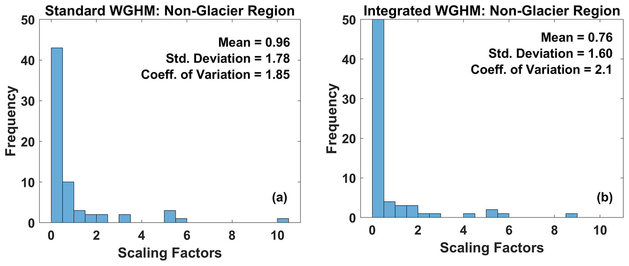
Figure 12 Frequency distributions of grid scaling factors from (a) standard and (b) integrated WGHM versions for the non-glaciated region of the Indus Basin. Notice the increased frequency of scaling factors <0.5 in the Integrated version.

Figure 12 shows the histograms of grid scaling factors only for the non-glaciated region of the Indus Basin (i.e., the non-glaciated pixels in Fig. 1). The increase in the frequency of small scaling factors (<0.5) and decrease in large ones (>3) indicates that the distribution of values from the integrated version is shifted towards zero as compared to the standard version. This shows that the addition of a localized water storage compartment in the model (glacier in this case) not only affects the scaling factors in that region but in the entire basin.

3.3.3 Frequency-dependent scaling factors

The frequency-dependent scaling factors for the Indus Basin are also shown in Table 3. For the trend component, the scaling factors from both versions (1.14 from standard and 1.23 from integrated) are almost identical to the frequency-independent basin-scale factors. This reinforces that the Indus Basin is dominated by long-term trends rather than seasonal signals, which causes the basin-scale factors to be driven by filtering the trend component. The scaling factors for the annual component from both versions (1.64 from standard and 1.59 from integrated) are significantly higher than 1 to account for leakage out of the annual mass changes described earlier. This also shows that the basin-scale factor alone would under-scale the annual component. The semi-annual scaling factors are nearly identical and close to 1 in the standard and integrated version, showing that filtering has a negligible effect on this component. These deviations from a single basin-scale factor reinforce the need for frequency-dependent scaling factors in basins where mass changes occur at different frequencies and the filtering has a significantly different effect on these individual frequencies.

Table 5 Parameters along with their formal uncertainties from time series fit to basin averages from scaled GRACE SH estimates under different scaling schemes. Also shown are corresponding parameters of DDC-corrected time series.

3.4 Scaled GRACE mass estimates

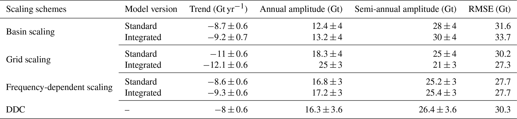
Table 5 shows the scaled GRACE time series parameters from each scaling scheme along with the corresponding values from an independent DDC approach. Trends become more negative (compared to −7.6 Gt yr⁻¹ from unscaled GRACE) from all three scaling schemes. Similar scaled trends from the basin and frequency-dependent scaling indicate the dominance of the trend component in the Indus Basin. Grid scaling leads to the most negative trends probably since grid cells with significant local mass changes contributing to the overall trend are scaled more with larger scaling factors than basin-averaged factors. All three scaling schemes restore the mass changes of annual frequency, lost due to filtering, as evident from increased annual amplitude (compared to 11.8 Gt from unscaled). Grid scaling seems to overestimate the annual amplitude when compared to frequency-dependent scaling. This overestimation is larger when using the integrated model. Across the schemes, scaling using the integrated model version leads to more negative trends and larger seasonal amplitudes than the standard version, except in the case of semi-annual amplitudes from grid scaling, which is reduced (compared to 24.8 Gt from unscaled). We studied these behaviors further in the simulation experiments and discuss their validity in detail in Sect. 3.5.

Different mass change components from grid-scaled GRACE from both model versions along with CSR MASCONS are shown in Fig. 13. We can see that even though MASCONS restore some signal, they do it in such a way that signal is added mostly where signal already was in the SH solutions (notice the corresponding pixels in panel 1 and 2 from left). Rescaling, on the other hand, can be seen to offer much more spatial contrast, driven by the spatial distribution of scaling factors. Therefore, rescaling can allow downscaling of GRACE resolution along with leakage correction if an ideal, perfect model were to be used. For example, MASCONS cannot separate the glacier loss trends in the upper Indus pixels from GW depletion trends in pixels in the southern part of Indus, while grid scaling from the integrated model does. However, the tendency of gridded scaling factors to be driven by the dominant mass change component in the pixels (trends or seasonal) may lead to incorrect spatial patterns for one or more of these components. This is discussed further in detail in Sect. 3.6.

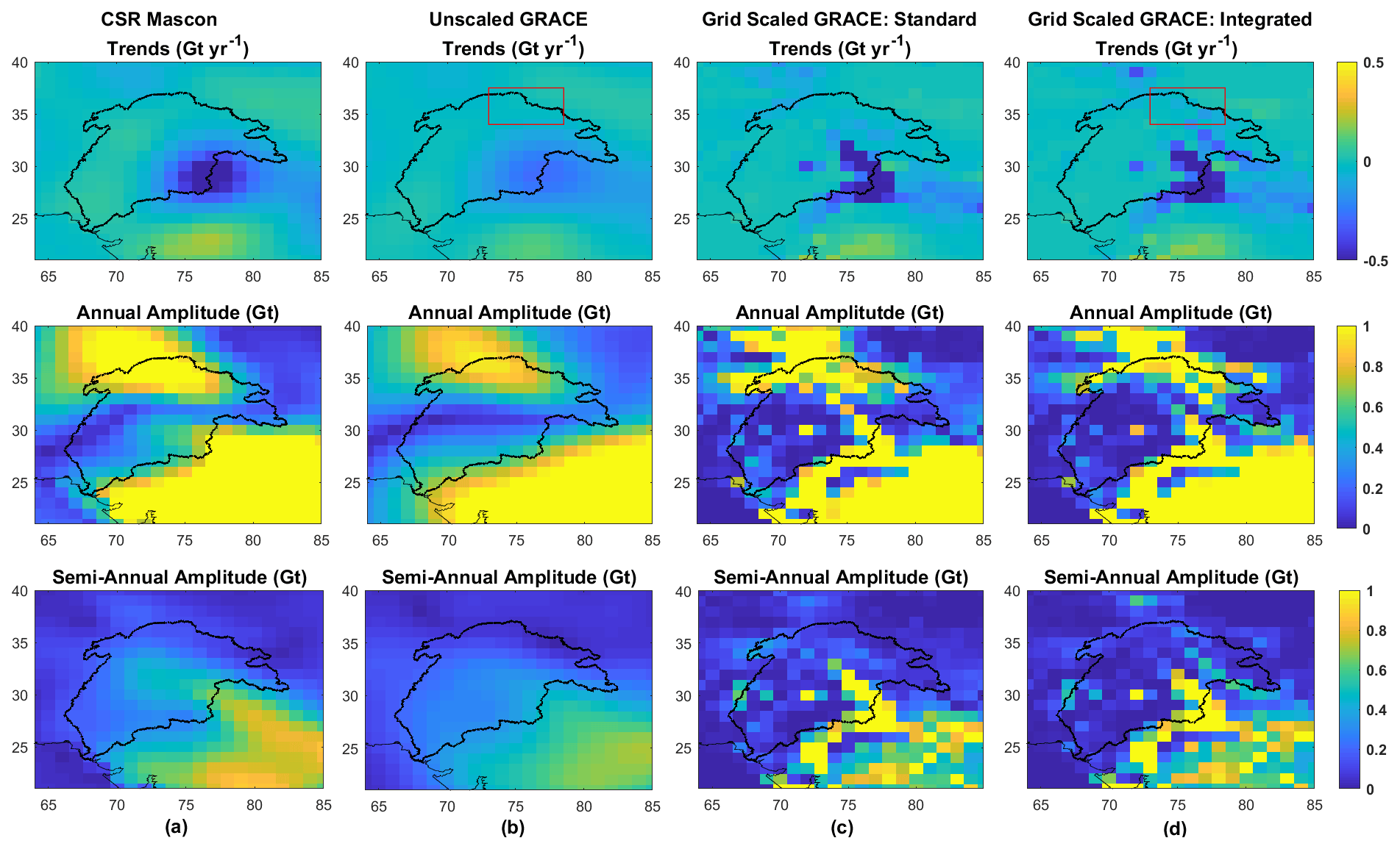
Figure 13 Spatial distributions of the components mass anomalies from (a) CSR MASCONS, (b) unscaled SH solutions, (c) grid-scaled SH solutions using standard, and (d) grid-scaled SH solutions using integrated WGHM (left to right panels) in the Indus Basin. The red bounding box indicates the extent of the Karakoram region.

The top row of trend maps in Fig. 13 also provides some interesting observations for a phenomenon known as the Karakoram Anomaly through the lens of GRACE. The “Karakoram Anomaly” is termed as the stability or anomalous growth of glaciers in the central Karakoram, in contrast to the retreat of glaciers in other nearby mountainous ranges of the Himalayas and other mountainous ranges of the world (Dimri, 2021). Various mass balances over this region have shown to be balanced or slightly positive (Farinotti et al., 2020). There is, however, significant uncertainty over the reasons for this anomaly which seems to be caused by the absence of reliable in situ observations in this region. However, GRACE observations of such small (nearly stable) trends will be contaminated with the nearby large negative trends due to leakage. This can be seen in Fig. 13 (top panel), where the red bounding box demarcates the extent of Karakoram (Dimri, 2021). The scaled trends for these pixels lying within the Indus Basin (top rightmost) are extremely small but negative (ranging from −0.01 to −0.1 Gt yr⁻¹). The uncertainty associated with these values is, however, nearly double. The two major limitations for the uncertainty of these values come from the inability of GRACE to resolve this extremely small signal from this phenomenon and the inability of the underlying integrated WGHM model to simulate this anomalous behavior at the current 1^∘ resolution, seen by large negative trends in the corresponding pixels (Fig. 7). However, scaling does seem to make a distinction between pixels of Karakoram with less negative trends and the adjacent pixels of Ladakh region with more negative trends, which cannot be seen in unscaled GRACE fields. We feel this to be a promising result indicating the presence of anomalous behavior in the Karakoram, but any further analysis is out of the scope of this study.

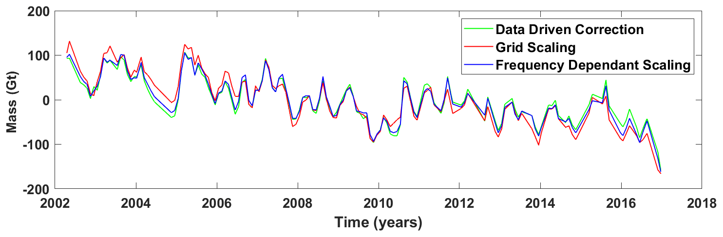
Figure 14 Basin-averaged GRACE time series for Indus Basin with corrected leakage using DDC, grid scaling, and frequency-dependent scaling using integrated WGHM.

Figure 14 depicts the basin-averaged GRACE time series from grid and frequency-dependent scaling using integrated WGHM compared to the DDC time series (Sect. 2.3.3).

Figure 14 shows that overall, frequency-dependent scaling using WGHM agrees exceptionally well with the independent DDC method for the Indus Basin. The agreement is also depicted in the time series components in Table 5. The small differences are well within the uncertainty limits and can be attributed to the methods being entirely different. Larger differences are, however, seen between grid scaling and DDC, which highlight the limitation of grid scaling to over- or under-scale certain pixels. Grid scaling can be seen to overestimate the trends compared to DDC since the trend-contributing pixels get scaled with larger scaling factors. Thus, this effect is seen to be more pronounced in grid scaling from the integrated version than from the standard version. The seasonal amplitudes have large differences, but their nature cannot be generalized between annual and semi-annual frequencies. This highlights the differences in physical processes governing the large-scale and fine-scale behavior of these components. These results provide confidence in the new frequency-dependent scaling using WGHM to restore the damaged signal at the catchment scale correctly.

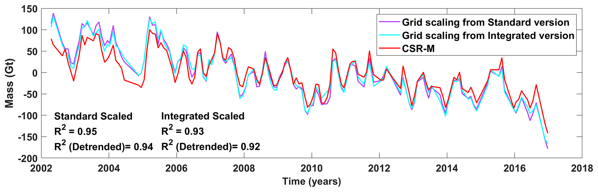
Figure 15 Comparison of basin-averaged time series from grid-scaled GRACE SH using standard, and integrated WGHM with basin-averaged time series from CSR-M.

A comparison of the grid-scaled GRACE SH time series to the MASCON time series (CSR-M) is shown in Fig. 15 to judge how realistic the values are. The R² values are similar to those obtained with unscaled GRACE SH, which provides confidence about the scaling factors obtained. We do not use this high value to judge the performance of scaling factors but only to highlight their numerical authenticity. A similarly high R² for the de-trended time series shows that the correlation is not spurious.

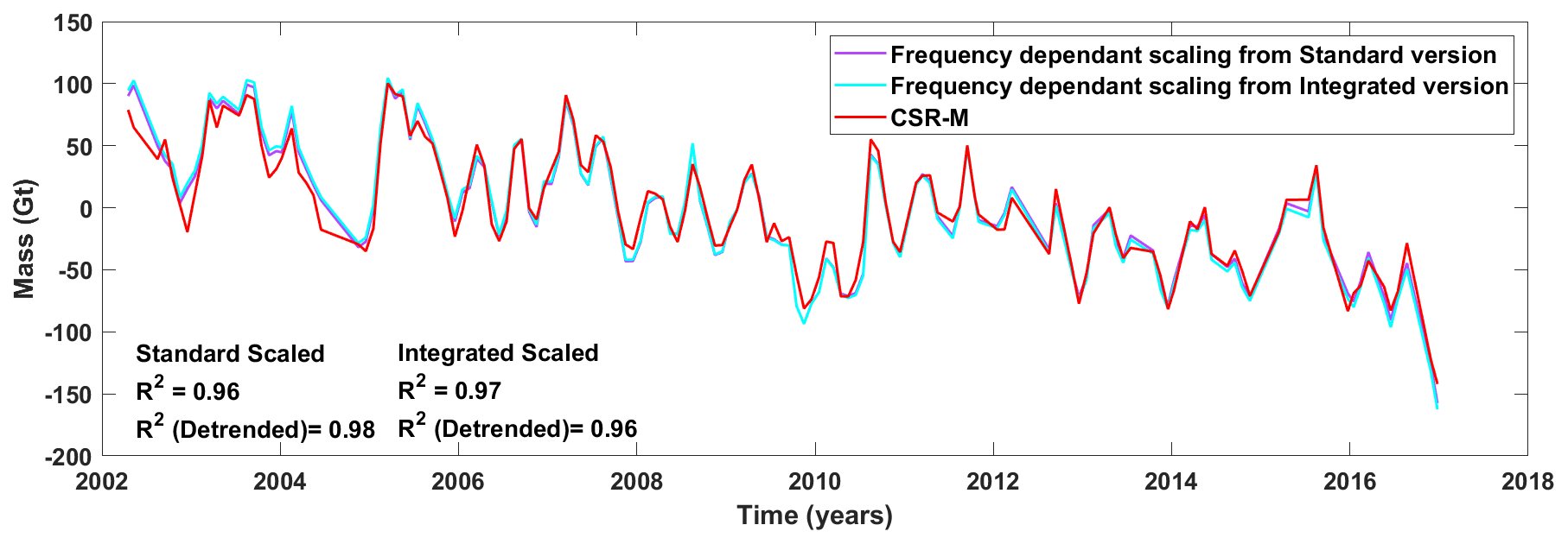
Figure 16 Comparison of basin-averaged time series from frequency-dependent scaling of GRACE SH using standard and integrated WGHM with basin-averaged time series from CSR-M.

Similarly, the result of frequency-dependent scaling is compared with the MASCON time series in Fig. 16. The obtained R² values are higher than those of grid scaling. This can be attributed primarily to the fact that the noise has not been scaled as in the grid scaling, making it more comparable to the MASCON time series. Even the real signals that may be present in the residual along with noise are not scaled. These real signals are mostly inter-annual, which are not much affected by filtering (Sect. 3.2), and hence not scaling them leads to a better correlation with the MASCON time series.

Table 6 Time series components of basin averages from the simulation using standard WGHM.

Table 7 Time series components of basin averages from the simulation using integrated WGHM.

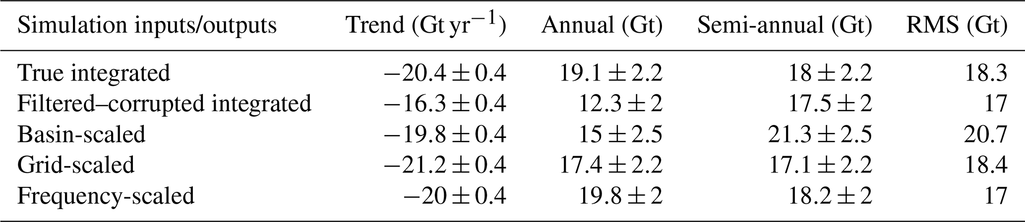
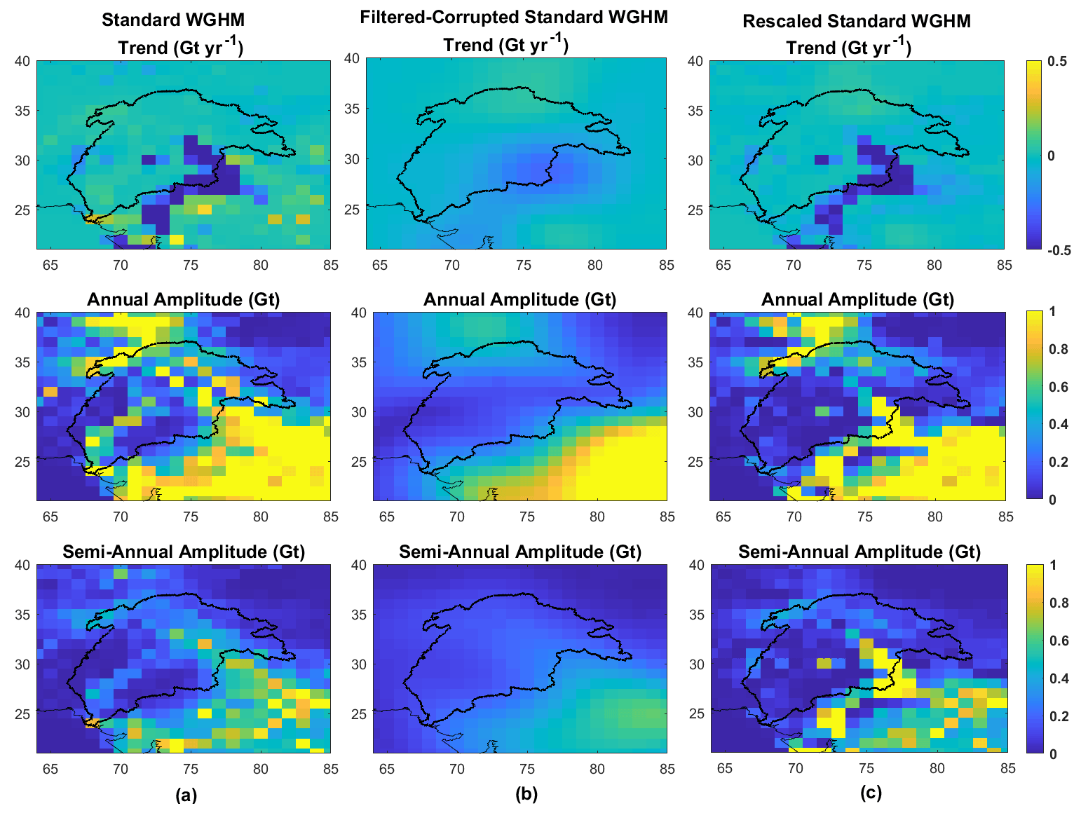
Figure 17 True (a) and recovered (c) spatial patterns of different mass change components from grid scaling of filtered–corrupted standard WGHM fields (b) in the simulation experiment.

Figure 18 True (a) and recovered (c) spatial patterns of different mass change components from grid scaling of filtered–corrupted integrated WGHM fields (b) in the simulation experiment.

3.5 Simulation experiments

The results of the simulations are shown in the form of time series components of the rescaled WGHM fields compared to the original true values in Table 6 for the standard version and Table 7 for the integrated version. The rescaled spatial fields from grid scaling compared to true fields are shown in Fig. 17 for the standard version and Fig. 18 for the integrated version.

The simulation experiments establish the frequency-dependent scaling as the best performing scheme in terms of recovering the true basin-averaged signal for both the model versions. The similarity of recovered trends from basin and frequency-dependent scaling supports the inference that the basin scaling factors are driven by the dominant mass change component, which is the trend in the case of the Indus Basin. The spatial pattern of the trend component is recovered extremely well by grid scaling. However, at the basin scale, recovered trends from grid scaling are more negative compared to the true trends since the pixels with large trends (Figs. 17 and 18; top left) are scaled with larger scaling factors (Fig. 10). The recovered semi-annual amplitude from grid scaling using integrated version is reduced, while increased using the standard version (compared to the corresponding filtered–corrupted semi-annual component). This supports the behavior seen in scaled GRACE with the following explanation: most of the semi-annual signal contribution comes from non-glaciated pixels in the trunk Indus and few pixels in the upper Indus (Figs. 17 and 18, bottom left). The scaling factors from the integrated version for the trunk Indus pixels are smaller than from the standard version, contributing to a decrease in semi-annual amplitude, while at the same time, the scaling factors are larger for the few upper Indus pixels, contributing to an increase (Figs. 17 and 18; bottom right). However, the greater number of trunk Indus pixels outweighs the increase in semi-annual signal of a few pixels of the upper Indus, leading to an overall decrease at the basin scale.

It can be seen (Tables 6 and 7) that grid scaling is unable to recover the true annual signal using both model versions, falling short by 29 % in the case of standard and 8 % in the case of the integrated version. Similar to the case made for semi-annual amplitude, this is evident from Figs. 17 and 18, where the true spatial pattern of annual component is not recovered by scaling, contributed by greater loss from pixels in trunk Indus and smaller gain from pixels in upper Indus. This contradicts the behavior seen with scaled GRACE estimates where grid scaling overestimates the annual amplitude compared to frequency-dependent scaling (equivalent to true amplitude). The above reasoning fails to explain the contradiction. However, comparing the spatial pattern of unscaled GRACE annual amplitude in Fig. 13 (second panel from left) with the pattern of annual amplitude in filtered–corrupted models in Figs. 17 and 18 (middle panel), it can be observed that the pixels from GRACE in the upper Indus Basin already hold much stronger annual signal compared to the corresponding pixels from the filtered–corrupted models. Therefore, larger scaling of these pixels is able to compensate for the loss from trunk Indus pixels, leading to an overall increase at basin scale (again, compared to frequency-dependent scaling).

Table 8 Noise and initial leakage error in unscaled GRACE basin-averaged time series of Indus Basin.

Table 9 Scaled noise and residual leakage in scaled GRACE basin-averaged time series of Indus Basin.

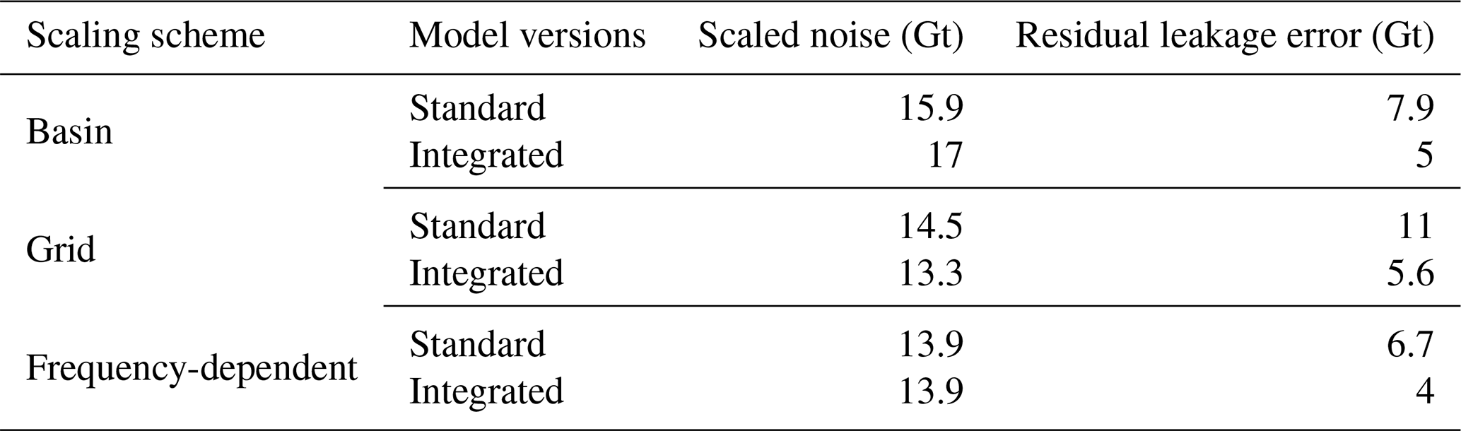
3.6 Residual leakage and scaled noise estimates

Table 8 shows the initial leakage error and the noise level in the unscaled GRACE basin averaged time series containing the random component of leakage. The initial leakage error determined from the standard version is less than that determined from the integrated version due to the smaller magnitude of TWS anomalies. The unscaled noise provides a baseline measure against scaled noise levels to evaluate the effect of scaling on random leakage components.

The scaled noise levels and the residual leakage errors from all three scaling schemes are shown in Table 9. These scaled noises implicitly contain the scaled random component of leakage, as explained in Sect. 2.3.3. Compared to unscaled GRACE (Table 8), the basin and grid scaling cause the noise to be scaled along with the signal, whereas frequency-dependent scaling does not affect noise. Grid scaling leads to lower noise than basin scaling due to the suppression of random errors in most of the Indus Basin regions where smaller scaling factors are present. Even smaller gridded scaling factors from the integrated version in those regions may explain the lower scaled noise. Basin scaling from the integrated version leads to higher noise than basin scaling from the standard version due to the higher magnitude of the scaling factor.

The residual leakages (Table 9) are least in frequency-dependent scaling, indicating its better performance. Residual leakages from grid scaling indicate their inability to reproduce the spatial pattern of seasonal signals in the basin. We must caution that although the residual leakage from grid scaling using the integrated version is lower, it is only because of the small magnitude of scaling factors. The underlying spatial patterns are no better recovered compared to grid scaling from the standard model.

4 Summary and conclusion

The study aimed to derive and evaluate scaling factors for the Indus River basin from WGHM 2.2d using its standard and integrated versions, to account for the leakage effects in mass estimates derived from GRACE spherical harmonic solutions. Scaling factors were derived based on three schemes of different spatio-temporal characteristics: basin scaling factors that are spatially and temporally constant; gridded scaling factors that are spatially variable while temporally constant; and frequency-dependent scaling factors that are spatially constant and temporally variable. The results of the scaling approach were compared with an independent DDC approach at the basin scale and with CSR MASCONS at both grid and basin scales. Inferences were made in an inter-comparison framework evaluated by detailed simulation experiments designed using WGHM spatial fields as a proxy for true TWSA and GRACE errors derived using full error covariance information of the SH coefficients.

The new frequency-dependent scaling outperforms others in terms of recovering the true basin average signal (including all its components), as evident by the simulation results and residual leakage levels. Its excellent agreement with an independent DDC-based estimate shows that it can be a viable alternative as a leakage correction approach for the Indus Basin. The frequency-dependent scaling, as proposed here, keeps the noise levels unscaled, which can provide robust estimates for practical applications that require accurate knowledge of the seasonal cycle of TWSA, such as water availability studies by decision-making bodies to ensure a safe supply of water to a region every year. If the users interested in other basins can determine additional dominant frequencies with sufficient confidence, then the frequency-dependent scaling can easily be applied to such frequencies.

Grid scaling allowed the recovery of the spatial pattern of trends but failed to capture the patterns associated with small seasonal amplitudes in the trunk Indus. It was found that with the integrated version, grid-scaled GRACE SH fields, unlike CSR MASCONS, could resolve negative trends from glacier mass loss in upper Indus from groundwater loss in the Indus plains. The addition of the glacier mass component modifying the scaling factors of the non-glaciated grid cells along with the glaciated grid cells is an interesting finding of the study. However, it was also found that the characteristics of basin averages of grid-scaled GRACE, such as trends and seasonal amplitudes, can be misleading in judging the performance of grid scaling due to over- and under-scaled pixels compensating, and leading to seemingly realistic basin-averaged values. Thus, we advise our readers to thoroughly assess the behavior of grid scaling for their basin of interest before directly using it for downstream applications.

The basin scaling scheme appears less sensitive to the model's mass distribution, which may justify the use of even worse models in their derivation. For the Indus Basin, basin scaling factors seem to be driven by the filtering effect on the trend and may be used for applications dealing with long-term trends in the basin. However, a better signal–noise separation must be achieved to minimize the scaling of noise. Frequency-dependent scaling shows that using a single basin scaling factor for basins like the Indus Basin with mass changes occurring at different frequencies will lead to inappropriate scaling of one or more of these components.

It is obvious to realize the possibility of a fourth gridded and frequency-dependent scaling scheme that would provide three scaling factors per grid cell. However, our initial experiments show that the time series decomposition at grid-scale leads to vastly varying annual and semi-annual components, and causes the scaling factors to be unrealistic. Hence, we leave that development for future studies. The study is limited in providing an external validation with independent TWS estimates. One approach is a comparison with TWS obtained from a water balance, but uncertainties in the derived TWS are much larger than the changes due to scaling. Hence, we stick to an inter-comparison framework along with simulation experiments that can be realistically reproduced and applied to different applications and studies that utilize GRACE data in the Indus Basin, and gain insights for choosing an appropriate scaling scheme per requirements. It may be stressed here that although the study has been done only for GRACE data, it can naturally be extended to the ongoing GRACE-FO observations (with the availability of the latest model outputs) without any loss of generality.