the Creative Commons Attribution 4.0 License.
the Creative Commons Attribution 4.0 License.
 | 19 Jul 2022
On the similarity of hillslope hydrologic function: a clustering approach based on groundwater changes
Fadji Z. Maina
Haruko M. Wainwright
Peter James Dennedy-Frank
Erica R. Siirila-Woodburn
Hillslope similarity is an active topic in hydrology because of its importance in improving our understanding of hydrologic processes and enabling comparisons and paired studies. In this study, we propose a holistic bottom-up hillslope clustering based on a region's integrative hydrodynamic response quantified by the seasonal changes in groundwater levels ΔP. The main advantage of the ΔP clustering is its ability to capture recharge and discharge processes. We test the performance of the ΔP clustering by comparing it to seven other common hillslope clustering approaches. These include clustering approaches based on the aridity index, topographic wetness index, elevation, land cover, and machine-learning that jointly integrate multiple data. We assess the ability of these clustering approaches to identify and categorize hillslopes with similar static characteristics, hydroclimate, land surface processes, and subsurface dynamics in a mountainous watershed – the East River – located in the headwaters of the Upper Colorado River Basin. The ΔP clustering performs very well in identifying hillslopes with six out of the nine characteristics studied. The variability among clusters as quantified by the coefficient of variation (0.2) is less in the ΔP and the machine learning approaches than in the others (> 0.3 for TWI, elevation, and land cover). We further demonstrate the robustness of the ΔP clustering by testing its ability to predict hillslope responses to wet and dry hydrologic conditions, of which it performs well when based on average conditions.
- Article
(17172 KB) - Full-text XML
- BibTeX
- EndNote


The ability to delineate areas into spatially defined regions for their use in characterizing hydrologic flow and transport behavior is important for several reasons, including the assessment, monitoring, and modeling of water quantity and quality. Hillslopes are the scale at which hydrologic flow and transport processes can be tractably and frequently measured. It is also the scale at which flow and travel time are quantified and the instrumentation, conceptualization, and modeling of hydrologic processes occur (Fan et al., 2019, Wainwright et al., 2022). While advancements have been made in the general understanding of hillslope dynamics over the last several decades, there is yet to be a globally agreed-upon classification and/or clustering for this important scale of interest in hydrology (McDonnell and Woods, 2004). Hydrologic signatures within hillslopes are the result of several simultaneous and nonlinear above- and below-ground processes. The uniqueness of a given location's characteristics (for example, the topography, geology, and vegetation) limits our ability to draw general hypotheses and to develop a similarity framework (Beven, 2000). Nevertheless, a classification is needed to provide guidance on catchments and hillslopes comparisons (McDonnell and Woods, 2004), paired studies (Andréassian et al., 2012; Bosch and Hewlett, 1982; Brown et al., 2005), and improve our understanding of the changes in hydrologic processes across the world. Further, hillslope similarity is potentially an important step toward developing reduced-order models and machine learning algorithms, where identifying regions based on their similarities can substantially reduce computational costs (Chaney et al., 2018). The scaling of hillslope to catchment classifications can also be useful in the prediction of hydrologic behavior in ungauged basins (Sivapalan et al., 2003), an exceedingly important challenge.
Hillslope similarity clustering approaches include the topographic wetness index (TWI) (Beven and Kirby, 1979), which was proposed to quantify the topographic control on hydrology as topography plays a key role in the movement of water. Many other variants of this index have been later proposed to improve the definition of topographic similarity (Grabs et al., 2009; Hjerdt et al., 2004; Loritz et al., 2019). Other clustering approaches are based on hydroclimate (Carrillo et al., 2011), soil type and texture (Bormann, 2010), and land cover type (e.g., forest, urban; Wagener et al., 2007). These indices assume that hillslopes with similar topography and land cover will have similar hydrologic responses. However, given that hydrologic processes are governed by many characteristics of the hillslope, clustering approaches relying on multiple landscape characteristics have also been proposed (Aryal et al., 2002; Sawicz et al., 2011). These top-down clustering approaches assume that areas with similar physical characteristics will lead to similar hydrologic processes (Oudin et al., 2010). Other clustering approaches use a bottom-up approach, where similarity is based on the hydrologic process. This clustering allows the estimation of the “hidden” hillslope characteristics, such as soil texture and geology that may drive similar hydrologic responses (Carrillo et al., 2011). Among the process-based clustering approaches existing in the literature, we can cite the Péclet number characterizing the diffusive and advective transfer of water at a hillslope scale (Berne et al., 2005; Lyon and Troch, 2007, 2010) and the catchment seasonal water balance (Berghuijs et al., 2014). Other authors have derived hillslope similarities from subsurface flow dynamics (Harman and Sivapalan, 2009).
One challenge in developing a similarity framework is the inherent heterogeneity of a given hillslope. For example, snow water equivalent (SWE), infiltration (I), and actual evapotranspiration (ET) distributions can range over an order of magnitude within a single hillslope (Wainwright et al., 2022). Defining a single integrative measure that can capture this spatio-temporal variability is difficult. However, groundwater fluctuations are often tightly linked to seasonal changes in climate and have been shown to play an important role in surficial processes such as ET (Maina et al., 2022; Maina and Siirila-Woodburn, 2020; Maxwell and Condon, 2016). Thus, groundwater measures may serve as a good proxy for the aggregated hydrologic response. Groundwater dynamics could help overcome the issue of uniqueness of place because even if there are strong differences in the characteristics of the hillslope, the integrated response may be similar, as some of the processes might not be important. Finally, the implications of groundwater changes are also important. For example, many regions are characterized by groundwater-dependent ecosystems or are hypothesized to have water table fluctuations affecting bedrock weathering rates and therefore, the concentration and fluxes of metal and nutrient exports (e.g., Winnick et al., 2017).
In this study, we define a holistic bottom-up hillslope clustering using the integrative hydrologic response quantified by the seasonal changes in groundwater levels. A caveat to this clustering is that groundwater dynamics are difficult to quantify and their measurements are frequently scarce. Hence, there are very few studies that use this variable to develop a hillslope similarity classification (Aryal et al., 2002; Lyon and Troch, 2007). However, today, thanks to advances in integrated hydrologic modeling (Brunner and Simmons, 2012; Maxwell and Miller, 2005), accurate quantification of the groundwater dynamics at high resolution in both time and space and their interaction with the key land surface processes and features is now feasible. These models (e.g., HydroGeoSphere, Brunner and Simmons, 2012; ParFlow, Maxwell and Miller, 2005; Advanced Terrestrial Simulator, Coon et al., 2016) that can be constrained with ground observations and measurements at ultra-high resolutions through aerial or remote sensing (i.e., drones, planes, or satellites) account for the two-way interactions between groundwater and land surface processes. Spatially resolved hydrologic flow models also enable us to jointly quantify other hydrologic variables useful to identify hillslopes with similar hydrologic responses, namely, trends in ET, SWE, and I. Nevertheless, we acknowledge that groundwater dynamics in some regions such as arid areas could be disconnected from land surface processes and less dependent on many key physical features of the hillslope, which may impede the ability of the proposed clustering in these regions.
We test the proposed hillslope clustering on the site of the Department of Energy's (DOE) Watershed Function Scientific Focus Area (SFA) located in the headwaters of the Upper Colorado River Basin. The East River watershed is not only representative of many headwater catchments in the western United States in terms of its spatial heterogeneity of above and below-ground characteristics, but also serves as an important proxy of water quantity and quality trends, which ultimately impact a large population of water supply in the western United States for municipal, agriculture, and industrial use (Hubbard et al., 2018). We test the robustness of the proposed hillslope clustering by comparing it to seven other common hillslope clustering approaches based on the aridity index (AI), TWI, elevation, land cover, and machine-learning approaches that jointly integrate multiple input data layers, such as elevation, land cover, and geology, and model outputs including ET and SWE. We assess the ability of these clustering approaches to identify and categorize hillslopes with similar physical characteristics (land cover and elevation), hydroclimate (precipitation and temperature), land surface processes (ET and SWE), and subsurface dynamics (soil saturation, water table depth (WTD), and seasonal changes in groundwater). We aim to provide answers to the following questions:
-
What are the best clustering approaches for identifying hillslopes with similar hydrologic processes?
-
Is a similarity index based on the seasonal groundwater variations sufficient to capture all the complex processes taking place at a hillslope scale?
2.1 Modeling framework
2.1.1 Selected integrated hydrologic model: ParFlow–CLM
We use the integrated hydrologic model, ParFlow, which has the advantages of simulating the water and energy balance from the bedrock to the lower atmosphere and therefore, connects groundwater dynamics with land surface processes. ParFlow solves the subsurface flow using the three-dimensional mixed form of the Richards equation (Richards, 1931), given by the following equation:
where SS is the specific storage [L−1], SW(ψP) is the degree of saturation [–] associated with the subsurface pressure head ψP [L], t is the time [T], ϕ is the porosity [–], kr is the relative permeability [–], z is the depth [L], qs is the source/sink term [T−1], and K(x) is the saturated hydraulic conductivity [L T−1], which is assumed to be a diagonal tensor with entries given as kx(x), ky(x), and kz(x). In this work, we assumed that the domain is isotropic and that the tensor is equal to 1 for all the three directions at each cell of the discretized model. In the unsaturated zone, both SW and kr depend on the ψ. The relationships between SW and kr and ψ are described by the van Genuchten model (van Genuchten, 1980).
Overland flow (Eq. 2) is solved by the kinematic wave equation in two dimensions:
where ψ0 is the ponding depth, ||ψ0,0|| indicates the greater term between ψ0 and 0, υ is the depth averaged velocity vector of surface runoff [L T−1], and qr is a source/sink term representing rainfall and evaporative fluxes [L T−1]. Surface water velocity at the surface in x and y directions, (υx) and (υy), respectively, is computed using the following set of equations:
where Sf,x and Sf,y friction slopes along x and y, respectively, and m is the Manning's coefficient. ParFlow employs a cell-centered finite difference scheme along with an implicit backward Euler scheme and the Newton–Krylov linearization method to solve these nonlinear equations. The computational grid follows the terrain to mimic the slope of the domain (Maxwell, 2013).
ParFlow is coupled to the Community Land Model (CLM, Dai et al., 2003), which allows for the simulation of important land surface processes such as ET and SWE, and the quantification of water leaving or entering the surface and subsurface (qs and qr, respectively, in the Richards and kinematic wave equations). CLMs model the thermal processes by closing the energy balance at the land surface given by
where Rn is the net radiation at the land surface [W m−2], a balance between the shortwave and longwave radiation, LE is the latent heat flux, [W m−2] which captures the energy required to change the phase of water to or from vapor, H is the sensible heat flux [W m−2], and G is the ground heat flux [W m−2]. All terms are a function of θ , the water content, which is computed by ParFlow.
Computing the different components of the energy balance requires meteorological forcing, vegetative parameters, and soil moisture. The latter is computed by ParFlow using Eqs. (1) and (2). Meteorological forcing includes precipitation, temperature, east to west and north to south wind speed, longwave and shortwave solar radiation, air pressure, and relative humidity. Vegetative parameters include maximum and minimum leaf area index, stem area index, aerodynamic roughness height, optical properties, stomatal physiology, roughness length, and displacement height. More details about the coupling between ParFlow and CLM and the equations governing the snow dynamics and ET can be found in the following papers: Jefferson et al., (2015), Maxwell and Miller (2005), and Ryken et al. (2020). ParFlow–CLM has been used in many studies to understand the interactions between groundwater dynamics and lower atmosphere (Maina et al., 2022; Maina and Siirila-Woodburn, 2020) at different scales from watershed (Foster and Maxwell, 2019; Maina et al., 2020) to continental scale (Maxwell and Condon, 2016).
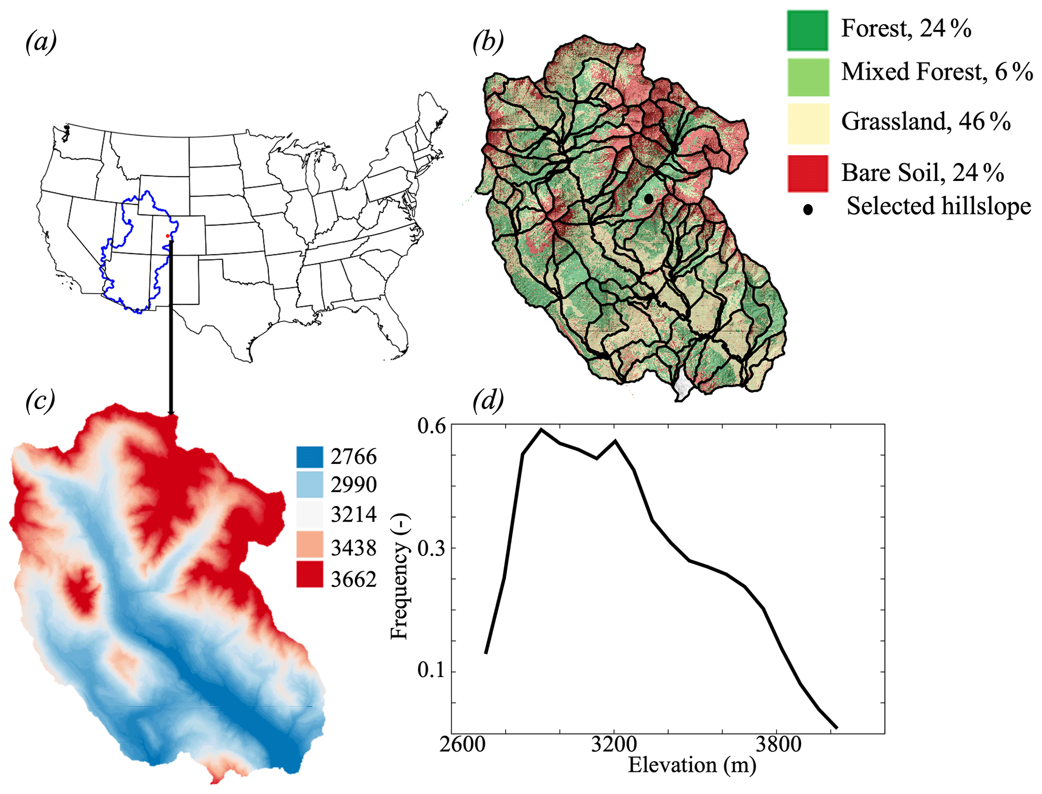
Figure 1(a) Location of the East River watershed, (b) land cover (NEON data set, 2020), (c) lidar digital elevation, and (d) elevation distribution within the East River.
2.1.2 East River watershed model setup
The East River watershed (Fig. 1), located in the Upper Colorado Basin, is one of the two major tributaries that form the Gunnison River, which, in turn, accounts for just under half of the Colorado River's discharge at the Colorado–Utah border. The total area of this watershed is approximately 255 km2 and the elevation varies from approximately 2700 to 3900 m. The watershed is characterized by strong heterogeneities in vegetation, geomorphology, and bedrock composition (Hubbard et al., 2018). The vegetation includes grasses, conifers, mixed conifers, aspens, and meadows, and lies on a complex geologic terrain, which is comprised of a diverse collection of Paleozoic and Mesozoic sedimentary and unconsolidated rocks. The watershed is also characterized by a strong hydroclimate gradient. The average precipitation is 1200 mm yr−1, while the average temperature is around 0 ∘C. Because of its very low cold winter with temperature below 0 ∘C, most of the winter precipitation is in the form of snow.
ParFlow–CLM used here is based on a previous version of the East River watershed model, as described by Foster and Maxwell (2019). Five layers constitute the model in the vertical direction, with varying thickness from 0.1 m at the land surface to 21 m at the bottom of the domain. The land use and land cover are derived from the high-resolution airborne remote sensing NEON campaign (Chadwick et al., 2020; Falco et al., 2020; Goulden et al., 2020). From the hyperspectral spectrometer and lidar readings, four major types of land cover are grouped as follows: forests (i.e., conifers and aspens), mixed forests, grasses, and bare soil. Parameterization of these different land cover types is derived from the International Geosphere–Biosphere Programme (IGBP) database (IGBP, 2018).
The subsurface of the study area is heterogeneous in both vertical and horizontal directions. The subsurface of the top 1 m corresponds to three soil layers as defined by the Soil Survey Geographic Database (SSURGO) database, and then corrected based on the land cover and geologic maps to include the outcropping of the bedrock. Two main types of soil are distinguished within the area: sandy loam and clay loam. The geology of the subsurface between 1 and 8 m below the ground was defined with United States Geological Survey (USGS) maps, which were further improved by local knowledge by Pribulick et al., (2016). This subsurface region is highly heterogeneous with different formations such as crystalline, sedimentary rocks, unconsolidated rocks, alluvial deposits, and debris flow. The bottom layer of the domain (extending from 8 m below the ground surface to the bottom of the model) is assumed homogeneous and represents the fractured bedrock.
We simulated the water year (WY) of 2015, which was a relatively average WY in the region based on average precipitation and temperature patterns. The meteorological forcing of the model has a resolution of an hour and is derived from two gridded data sets: Parameter-elevation Regressions on Independent Slopes Model (PRISM) and North American Land Data Assimilation System (NLDAS). The PRISM data set (Daly et al., 2008) is used for precipitation and temperature because of its accuracy and high spatial resolution (800 m). However, the daily resolution of PRISM impedes its ability to be used to reproduce diurnal cycles, an important factor when studying land surface processes requiring hourly forcing. Phase 2 of the North America Land Data Assimilation System NLDAS-2 forcing (Cosgrove et al., 2003), on the contrary, provides hourly changes in precipitation and temperature, yet is only available at coarser ∘ resolutions. As such, we employ a mass-conservative temporal interpolation, which disaggregates the total daily PRISM precipitation into an hourly time series, based on the signal of the NLDAS-2 precipitation and temperature trends. For the other forcing variables (i.e., shortwave and longwave radiation, wind speed, atmospheric pressure, and specific humidity), we use NLDAS-2 forcing, (Cosgrove et al., 2003). Simulated river stages and SWE were compared to observations in previous studies (Maina et al., 2022; Foster and Maxwell, 2019). Groundwater measurements are scarce in the watershed and the majority of the measurements are performed near a station measuring changes in river stages. Therefore, river stages and groundwater measurements at this point provide similar information.
2.2 Hillslope delineation
As shown in Fig. 1b, 127 hillslopes are delineated in the East River watershed based on the elevation following Noël et al., (2014) and using Topotoolbox developed by Schwanghart and Scherler (2014). A threshold of flow accumulation was set to match the stream observations at major tributaries of the East River (Carroll et al., 2018). Because the hillslope delineation could be sensitive to the threshold of the drainage area, we tested different threshold values to find that the selected threshold value (810 000 m2) represents the scale of hillslope at which the within-hillslope variability of key properties (such as elevation and aspect) is minimized and hillslope-averaged properties can account for the majority of watershed-scale variability (Wainwright et al., 2022).
2.3 Hillslope clustering approaches
We use eight hillslope clustering approaches:
-
The ΔP1 clustering proposed in this study identifies hillslopes with similar groundwater dynamics. Figure 2 shows the temporal variations of the simulated SWE and WTD at a selected hillslope (see its location in Fig. 1). All hydrologic variables have been computed at a hillslope scale by computing the arithmetic average of all cells in each hillslope. In this mountainous watershed where the largest changes in WTD are mostly a result of snowmelt, WTD decreases from the beginning of the WY (i.e., October) to the beginning of snowmelt (i.e., starting from April). As the snow starts to melt and precipitation starts to fall as rain instead of snow, WTD starts to rise. The shallowest WTD is June and July when the snow has completely melted and has had time to percolate through the unsaturated zone into the groundwater. This period also corresponds to the period of high ET, because both the evaporative demand and the water availability are high.
The dynamics show two periods that characterize the dynamics of the hillslope: from the initial conditions to the baseflow conditions when the hillslope is losing water, then from baseflow conditions to the peak of WTD when the hillslope is gaining water. To characterize these groundwater dynamics, we define two variables:
-
ΔP1 represents the change in WTD between the beginning of the water year and the deepest WTD during the baseflow conditions. This variable quantifies the amount of water released by the hillslope during the dry period at the beginning of the water year. It thus contains information about the amount of water that the hillslope typically releases/loses, mainly by ET and discharge, given its physical characteristics and climate dynamics.
-
ΔP2 represents the changes in WTD between the peak flow (i.e., the period with the shallowest WTD) and the baseflow conditions. ΔP2 quantifies the amount of water gained in the hillslope by recharge and thus contains information about the recharge ability of the hillslope given its physical characteristics and climate dynamics.
These two key variables allow us to quantify water release (ΔP1) and recharge (ΔP2) within a hillslope; two key dynamics of the watershed hydrologic function (Sivapalan, 2006; Wagener et al., 2007, Wainwright et al., 2022). We note that these dynamics are also illustrated by the changes in measured groundwater levels as depicted in Appendix A.
-
-
Elevation: in mountainous watersheds, because the differences in hydroclimate are primarily driven by elevation, hillslopes with similar elevations could potentially have similar land surface processes signatures.
-
Land cover: hillslopes can also be clustered by their dominant land cover. Land cover shapes land surface processes, which in turn affect subsurface dynamics and the water balance at the hillslope scale.
-
TWI: The topographic wetness index commonly used to cluster hillslopes is given by , where α is the upslope draining area and β is the local angle.
-
AI: the AI (ETP/precipitation, where ETP is the potential evapotranspiration) represents the ratio of the average demand for moisture to the average supply of moisture. We derive the spatial distribution of the AI in the East River from the Global Aridity Index data set (CGIAR-CSI, 2019).
-
Machine-learning-based clustering: we define the hillslope similarity using the clustering of ParFlow–CLM input and output data layers. Clustering was performed in three different ways using the following data: (1) model input (elevation, percentage of the main land cover type, TWI, and AI), referred to hereafter as the “clustering input” (C.I.) method, (2) model output (ET, SWE, WTD, and ΔP1), referred to hereafter as the “clustering output” (C.O.) method, and (3) both model input and output data layers, referred to hereafter as the “clustering input-output” (C.I.O.) method. We use hierarchical clustering, which is a decision-tree-based method that divides data points based on a series of binary splits (Devadoss et al., 2020; Kassambara, 2017; Wainwright et al., 2022). We define the linkage (or the distance) between any two clusters based on the Euclidian distance and the Ward method that computes the variance within each cluster, measuring the distance between each observation and the cluster's mean, and then taking the sum of the distances' squares.
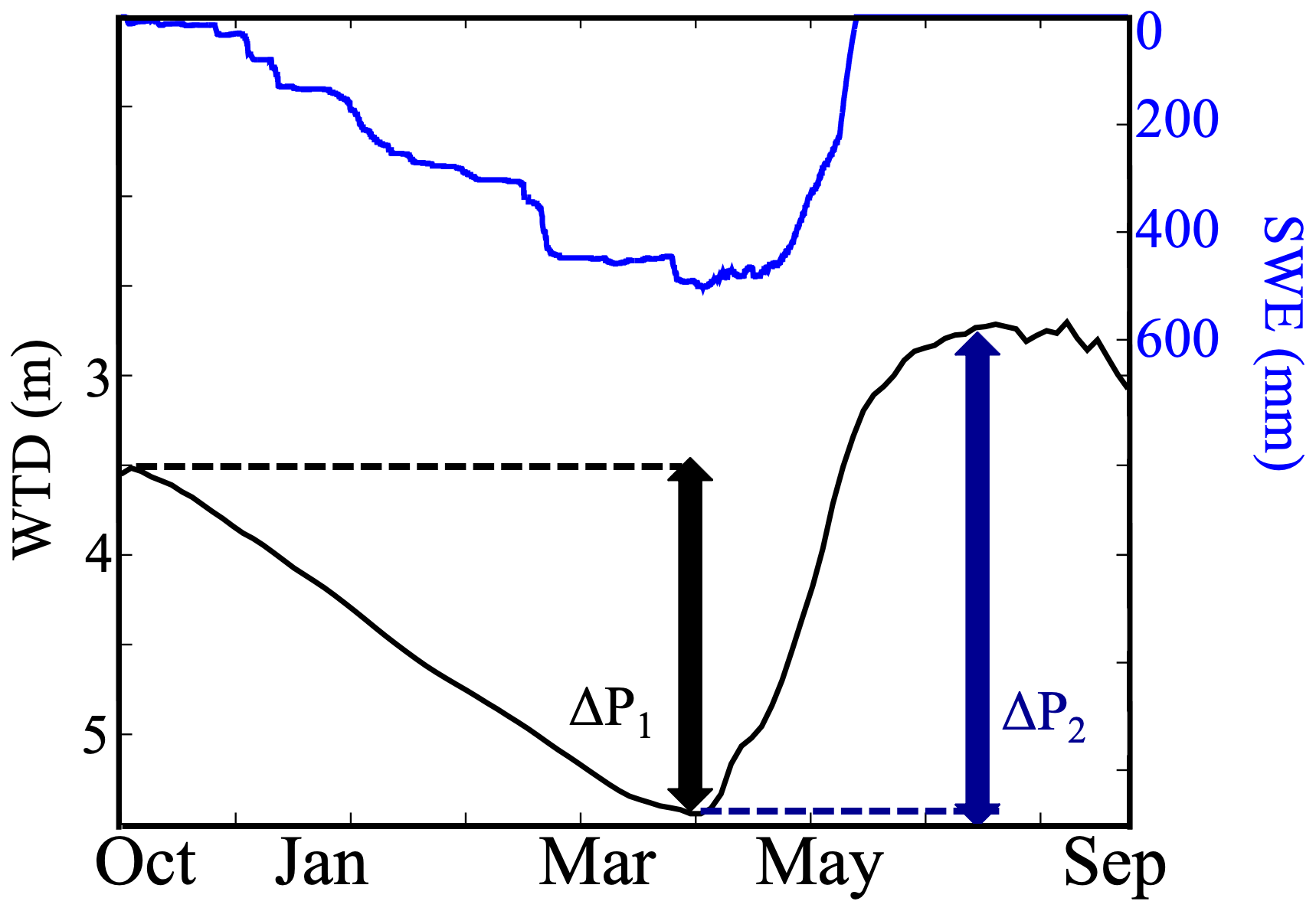
Figure 2Temporal variations of water table depth (WTD) and SWE at an example hillslope. The location of the hillslope is shown in Fig. 1.
2.4 Hillslope clustering comparisons
To test the ability of the eight selected clustering approaches to identify and categorize hillslopes with similar static characteristics and dynamics, we assess each clustering's ability to describe several characteristics of the hillslope. These are elevation, land cover, hydroclimate (i.e., precipitation), land surface processes (SWE and ET), and subsurface dynamics (WTD values and variations). For each clustering, we define three zones. For each variable, zone, and clustering, we compute the mean (μ) of the hillslope values and the corresponding coefficient of variation (CV). We also calculate the mean of the CV of the different zones for each variable and clustering.
3.1 Hillslope characteristics
Figure 3 shows the spatial distribution of hillslope temperature, precipitation, SWE, ET, WTD, and ΔP1.
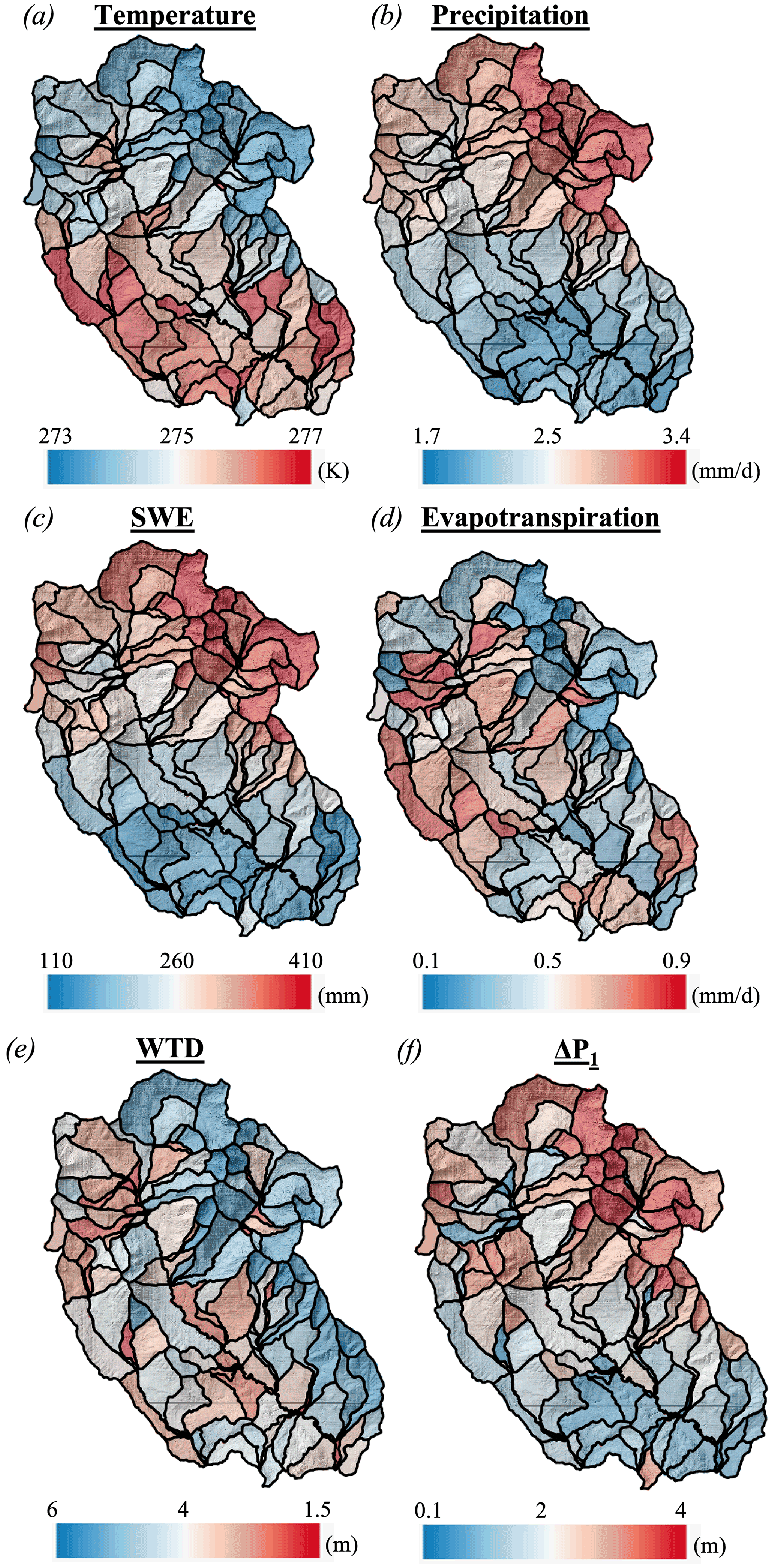
Figure 3Spatial distributions of hillslope annual average values of (a) temperature, (b) precipitation, (c) snow water equivalent (SWE), (d) evapotranspiration, (e) water table depth (WTD) and (e) ΔP1.
As expected, the hillslopes characterized by high SWE have high precipitation and low temperatures in contrast to the hillslopes with low SWE. However, ET shows a different pattern, as it depends on both water availability and ET demands, which depends on the type of land cover. The mid-elevation zone (i.e., Zone 2) with a high coverage of forests has high ET. Hillslopes with high ΔP1 have a deep WTD on average because the WTD increases significantly during baseflow conditions and reaches very large values as quantified by ΔP1. Hillslopes with high ΔP1 values generally correspond to hillslopes with high precipitation and low temperature and therefore, high SWE values.
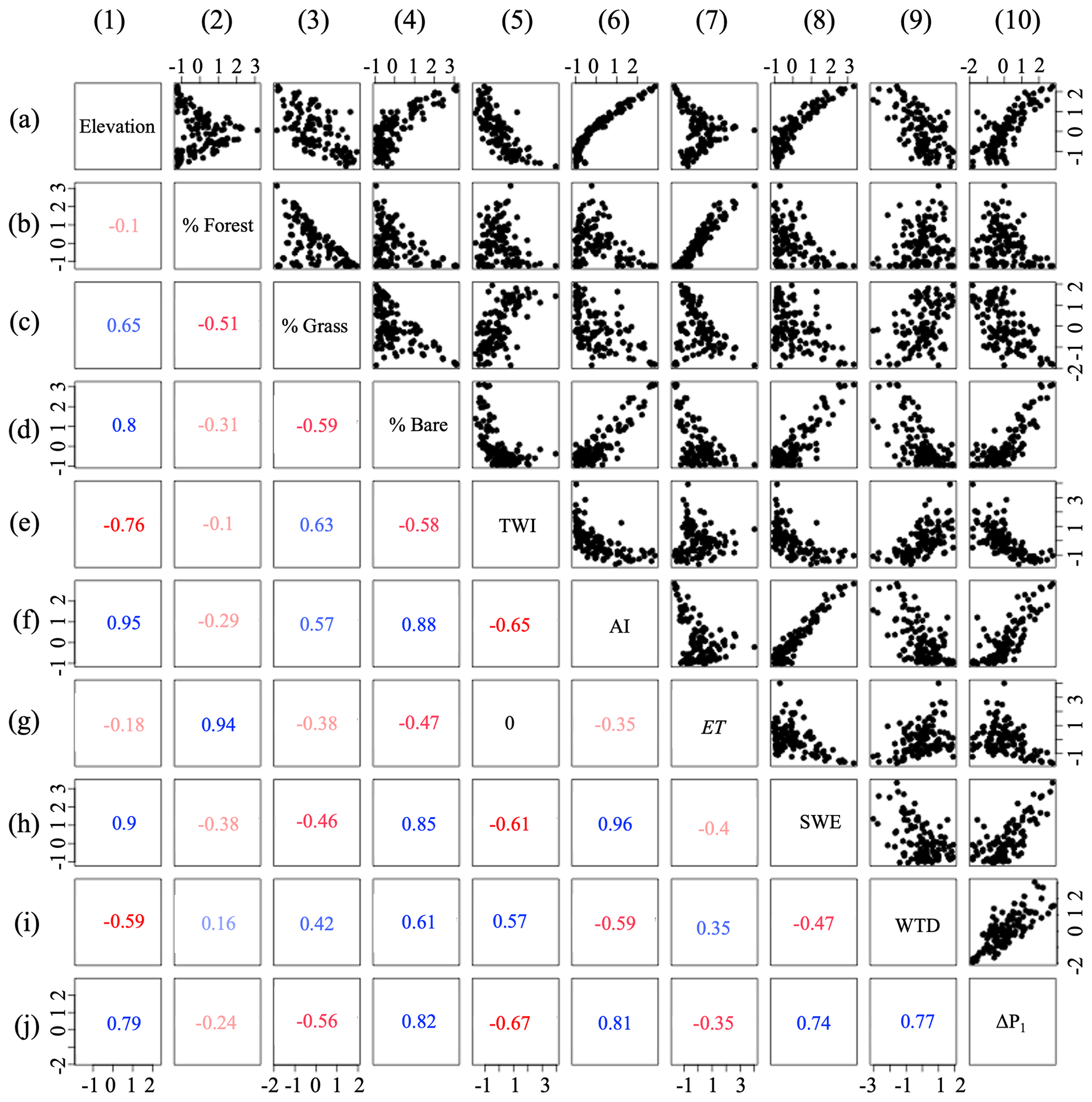
Figure 4Pearson's correlations between the selected variables for hillslope clustering approaches: elevation, percent of the main land cover type (forest, grassland, and bare soil), topographic wetness index (TWI), aridity index (AI), evapotranspiration (ET), snow water equivalent (SWE), water table depth (WTD), and seasonal changes in groundwater ΔP1. Note that correlation coefficients are color-coded based on their values.
To better understand the relationship between ΔP1 and the hillslope physical characteristics and hydrologic processes, we study the Pearson correlation coefficient between ΔP1 and the elevation, the percent of the dominant land cover, TWI, AI, ET, SWE, and WTD (Fig. 4).

Figure 5Spatial distribution of hillslope zones derived from the eight selected clustering approaches: (1) ΔP1, (2) elevation, (3) land cover (LULC), (4) topographic wetness index (TWI), (5) aridity index (AI), and clustering with (6) inputs, (7) outputs, and (8) input and output variables.
Results for ΔP2 are not shown because ΔP2 is strongly correlated to ΔP1. Bare soil, TWI, AI, SWE, and ΔP1 are strongly correlated (we define this as Pearson's correlation coefficient higher than 0.7) with elevation (Fig. 4, column 1, lines d, e, f, h, and j). In particular, elevation has a dominant control on AI and SWE, with a Pearson's correlation coefficient higher than 0.9. We observe nonlinearity such that TWI increases in the lower elevation and that AI becomes constant at the lower elevation. A high percentage of forest is only found in mid-elevation (Fig. 4, 2a), whereas a high percentage of grassland is well correlated to low elevations (Fig. 4, 3a). ET is positively correlated to the percent of forests (Pearson's correlation coefficient is higher than 0.9, Fig. 4, 2g). ΔP1 has a Pearson's correlation coefficient higher than 0.7 for 6 out of 9 studied variables (elevation, percent of bare soil, TWI (correlation coefficient equal to 0.67), AI, SWE, and WTD, Fig. 4, line j, columns 1, 4, 5, 6, 8 and 9). It therefore indicates that changes in ΔP1 can reflect the changes of these variables. The two variables with low correlations with ΔP1 are ET and the percent of forests (Fig. 4, line j, columns 2 and 7). ET is related to groundwater dynamics in a nonlinear way (Condon et al., 2013; Ferguson and Maxwell, 2010; Rahman et al., 2016). As shown in these studies, regions with shallow WTDs have the highest ET fluxes and this flux typically decreases significantly with WTD. When WTD reaches a critical depth, the groundwater and the atmosphere disconnect and changes in WTD do not impact ET.
3.2 Hillslope clustering
For each clustering, we identify three zones (Fig. 5). For the ΔP1, elevation, TWI, and AI clustering approaches, we define the thresholds of each zone by analyzing the distributions of the hillslope values of the following indices:
-
ΔP1: Zone 1 comprises hillslopes whose ΔP1 is less than 1.5 m, ΔP1 of hillslopes in Zone 2 are comprised between 1.5 and 2.5 m, and Zone 3 groups all hillslopes with ΔP1 greater than 2.5 m.
-
Elevation: Zone 1 characterizes low elevation areas (average hillslope elevation is less than 3000 m), Zone 2 is mid (average hillslope elevation comprises between 3000 and 3500 m), and Zone 3 is high elevation (hillslopes with an average elevation greater than 3500 m).
-
Land cover: Zone 1 describes hillslopes that have predominantly grasses as land cover, Zone 2 describes hillslopes with more than 50 % of forest, and Zone 3 describes hillslopes where bare soil is the dominant land cover.
-
TWI: we define 3 zones with high (TWI > 1, Zone 1), mid (TWI comprises between 1 and 0.2, Zone 2), and low (TWI < 0.2, Zone 3) TWI.
-
AI: Zone 1 comprises hillslopes with AI less than 0.45, Zone 2 describes hillslopes with AI between 0.45 and 0.55, and hillslopes of Zone 3 have an AI greater than 0.55.
-
Machine-learning-based clustering: the approaches automatically regroup the similar hillslopes into three zones.
Table 1Mean μ and coefficient of variation CV of each variable and hillslope zone derived from the eight clustering approaches. LULC stands for land cover and land use.

3.3 Comparisons of the eight selected hillslope clustering approaches
Table 1 depicts the mean (μ) and the corresponding coefficient of variation (CV) of hillslope values for each variable, zone, and clustering.
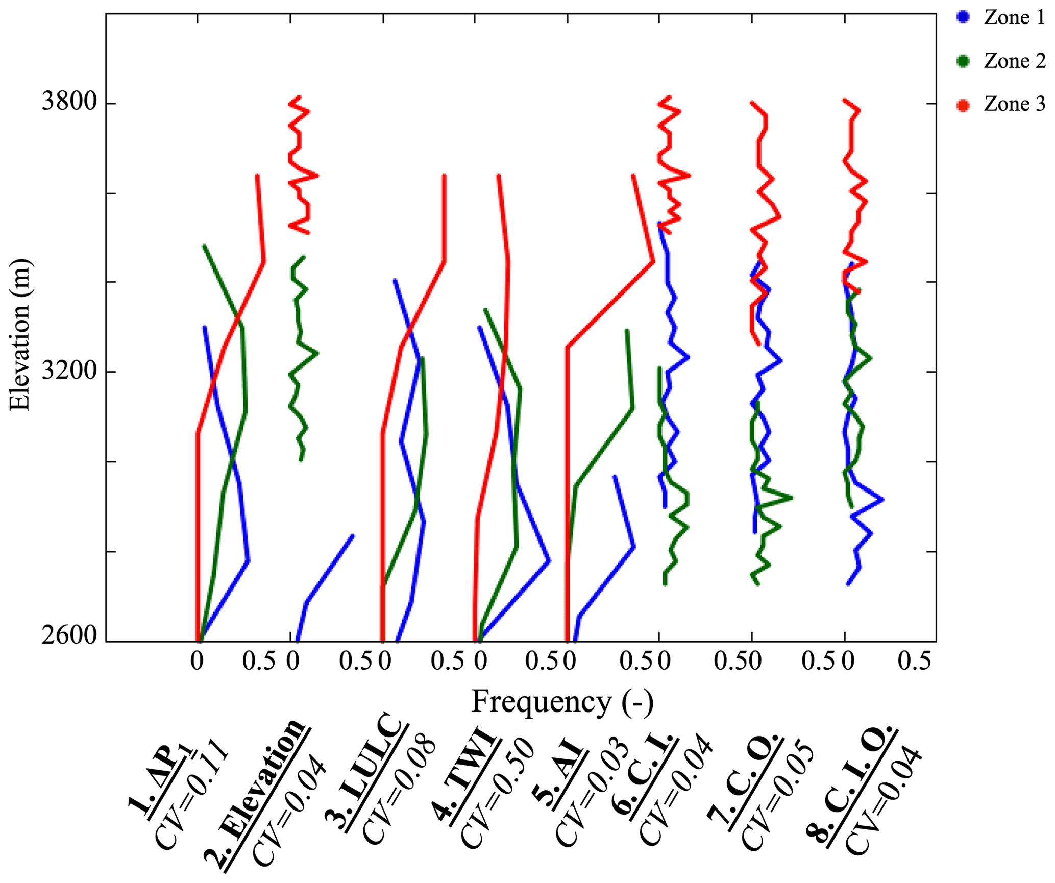
Figure 6Frequency distributions of hillslope elevation. Clustering approaches are based on ΔP1, elevation, land cover (LULC), topographic wetness index (TWI), aridity index (AI), and machine-learning approaches (with inputs C.I., outputs C.O., and inputs and outputs C.I.O.). Hillslope clustering approaches are located across the x axis. Note that we plotted the distributions of the eight clustering approaches on the same graph and between each dotted line (with a frequency from 0 to 0.5), the frequency distributions of the three zones derived from the clustering are plotted.
3.3.1 Similarities in hillslope structure
Elevation plays an important role in the hydroclimate of a region, especially in mountainous watersheds where it controls snow accumulation and controls the downstream hydrology. Figure 6 shows the elevation frequency distributions associated with the three zones derived from the eight clustering approaches.
By classifying the hillslopes using their similarity in ΔP1, we observe that hillslopes with low ΔP have the lowest elevation, while the hillslopes of Zone 3 (high ΔP1) have the highest elevation. Unsurprisingly, the second clustering (i.e., elevation) clearly identifies the hillslopes with similar elevation. The AI clustering also identifies hillslopes with similar elevation, as shown in Figs. 4 and 6. The TWI clustering performs moderately, where Zones 1 and 2 are characterized by similar elevation distributions. Hillslopes with lower TWI are mostly located in high elevation areas compared to the low elevation hillslopes. In the land cover clustering, most of the grassed hillslopes (Zone 1) are in low elevation, forests (Zone 2) are in mid-elevation, and hillslopes whose landscape is mainly bare soil (Zone 3) are in high elevation areas above the tree line. The three clustering approaches using machine learning allow the identification of hillslopes with similar elevation, as their coefficients of variation are of the same order as the elevation clustering.
Table 2Average values of the hillslope ratio of forests, grasslands, and bare soil for each zone and clustering.

Table 2 describes the average hillslope ratio of land cover type (forests, grassland, and bare soil) for each zone and type of clustering. The land cover clustering indicates that grassland is the dominant land cover of Zone 1, forests in Zone 2, and bare soil in Zone 3. Only the machine-learning clustering approaches using outputs lead to a similar conclusion, whereas while the other clustering approaches capture the characteristics of Zone 1 and 3, they do not identify a distinct forested Zone 2. For the ΔP1 clustering, this could be attributed to the disconnection between groundwater dynamics and land surface processes that takes place in certain forested zones. Since clustering based on landscape characteristics and ΔP1 do not identify such a distinct zone, it suggests that this zone may not be indicative of distinct hydrologic behavior.
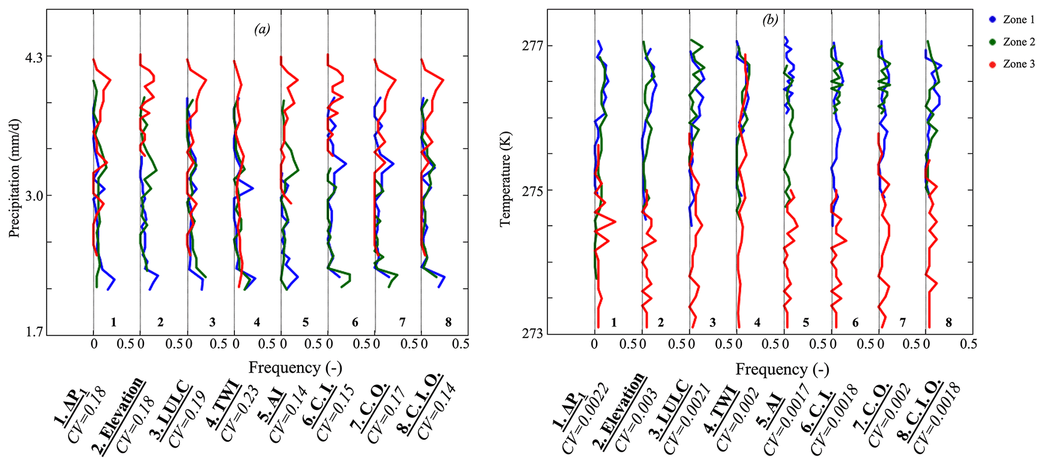
Figure 7Frequency distributions of hillslope (a) annual average daily rates of precipitation and (b) annual average temperature. Clustering approaches are based on ΔP1, elevation, land cover (LULC), topographic wetness index (TWI), aridity index (AI), and machine-learning approaches (with inputs C.I., outputs C.O., and inputs and outputs C.I.O.). Hillslope clustering approaches are located across the x axis. Note that we plotted the distributions of the eight clustering approaches on the same graph, and between each dotted line (with a frequency from 0 to 0.5), the frequency distributions of the three zones derived from the clustering are plotted.
3.3.2 Similarities in hydroclimate
Figure 7a and b depicts the distributions of precipitation and temperature obtained with the eight selected clustering approaches. The AI clustering allows the identification of hillslopes with a similar hydroclimate because they have low values of coefficients of variation. Zone 1, located in low elevation, has low precipitation and high temperatures, contrary to Zone 3. Zone 2 is characterized by a hydroclimate that is in between those of Zone 1 and 3. Our ΔP1 clustering leads to conclusions similar to the machine-learning-based clustering and AI. These three clustering approaches have the same average CV and are the only methods that allow the identification of hillslopes with a similar hydroclimate. However, we note that in the three machine-learning-based clustering and in the ΔP clustering, Zones 1 and 2 have a similar hydroclimate, which is not the case in the AI clustering. While the land cover clustering approaches clearly identify the typical hydroclimate of the hillslopes of Zone 3, the two remaining zones have the same hydroclimate. The TWI clustering does not identify hillslopes with a similar hydroclimate because it relies on the hydrologic processes driven by the topography. TWI shows that clustering that includes only hydroclimate would miss important information on distinct hillslope hydrologic processes that strongly affect the response of the hillslope to meteorological forcing.
3.3.3 Similarities in hydrologic processes
In this section, we study the ability of the selected clustering approaches to identify hillslopes with similar hydrologic processes, which are snow dynamics, evapotranspiration, and WTD values and variations.
Land surface processes
A robust clustering in mountainous watersheds should identify hillslopes with similar snow dynamics. Figure 8a illustrates the SWE frequency distribution associated with each zone and clustering. Because SWE dynamics are primarily driven by elevation and precipitation, the AI and machine-learning-based clustering have the lowest average of the CV, followed by the land cover and the ΔP1 clustering. The land cover spatial distribution contains information about elevation, especially in high elevation areas where some hillslopes are located above the tree line. The ΔP1 clustering accounts for SWE dynamics because ΔP1 is highly correlated to SWE, as discussed in Sect. 3.1.
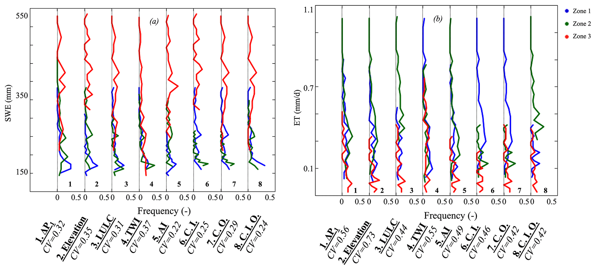
Figure 8Frequency distributions of hillslope land surface variables: (a) annual average SWE and (b) annual average daily rates of ET. Clustering approaches are based on ΔP1, elevation, land cover (LULC), topographic wetness index (TWI), aridity index (AI), and machine-learning approaches (with inputs C.I., outputs C.O., and inputs and outputs C.I.O.). Hillslope clustering approaches are located across the x axis. Note that we plotted the distributions of the eight clustering approaches on the same graph and between each dotted line (frequency from 0 to 0.5), the frequency distributions of the three zones derived from the clustering are plotted.
The spatial distribution of ET is controlled by many factors, including soil moisture, land cover, and subsurface flow. The land cover clustering performs well in identifying hillslopes with similar ET because the latter strongly depends on the land cover (Fig. 8b). Consistent with the aforementioned results, the other clustering approaches that perform well are the machine-learning-based clustering and the AI. The TWI and elevation clustering approaches do not separate hillslopes by their ET values because they do not account for varying land cover and soil properties that influence ET. The average CV of the ΔP1 clustering is close to those of the land cover and AI clustering. As stated in many studies (Ferguson and Maxwell, 2010; Maina and Siirila-Woodburn, 2020; Maina et al., 2022), subsurface flow affects ET as this information about subsurface flow contains valuable information about the ET, even if the correlation between ΔP1 and ET is nonlinear.
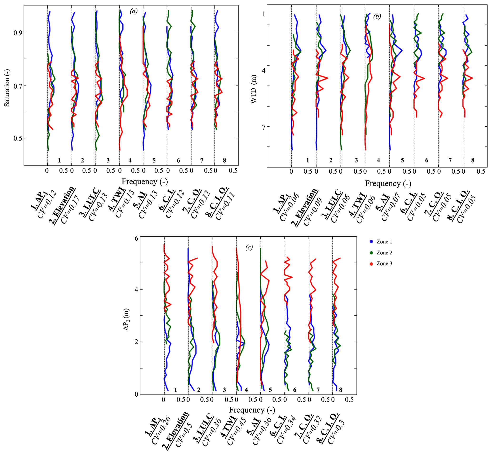
Figure 9Frequency distributions of hillslope (a) saturation, (b) WTD, and (c) ΔP2. Clustering approaches are based on ΔP1, elevation, land cover (LULC), topographic wetness index (TWI), aridity index (AI), and machine-learning approaches (with inputs C.I., outputs C.O., and inputs and outputs C.I.O.). Hillslope clustering approaches are located across the x axis. Note that we plotted the distributions of the eight clustering approaches on the same graph and between each dotted line (frequency from 0 to 0.5) the frequency distributions of the three zones derived from the clustering are plotted.
Similarities in subsurface hydrodynamics
We investigate the ability of the eight selected clustering approaches to identify hillslopes with similar subsurface hydrodynamics. We study the average saturation of the first 10 cm of the soil throughout the WY, the yearly average of WTD, and ΔP2. Soil saturation is a key feature in both subsurface and atmospheric dynamics; it controls ET and groundwater recharge. The average CV of the ΔP1, TWI, AI, land cover, and clustering approaches are very similar (Fig. 9a). As the land cover clustering adequately regroups hillslopes with similar ET, it also allows the regrouping of hillslopes with similar soil saturation. Because the TWI describes the characteristics that drive flow, it serves as a good indicator of soil saturation like the AI. Similar to the results above, the machine-learning-based clustering perform well. The ΔP1 clustering has a low average CV due to the strong connection between the changes in WTD and soil saturation. It is only the elevation clustering that fails to identify hillslopes with similar soil saturation, where the distributions of the three defined zones show overlap.
WTD is an important variable for determining groundwater storage. Here, we rely on the average WTD throughout the year. As expected, the ΔP1 clustering identifies hillslopes with similar WTD (Fig. 9b). Zone 1 located in low elevation has the shallowest WTD and the lowest ΔP1, contrary to Zone 3. Zone 2 exhibits a behavior that is in between those of Zone 1 and 3. The TWI and land cover clustering approaches also are good for identifying hillslopes with similar WTD. Hillslopes with low TWI (Zone 3) have the deepest WTD, contrary to the hillslopes of Zone 1. The TWI identifies hillslopes with similar WTD because of the high relief of the watershed that drives its hydrology (Fan et al., 2019). The land cover clustering indicates that most of the forest (Zone 2) and bare soil (Zone 3) hillslopes have deep WTD, whereas grass (Zone 1) hillslopes have the shallowest WTD. The elevation clustering does not accurately identify hillslopes with similar WTD and its average CV remains higher than the 4 other clustering approaches. The AI, like the elevation, is not a good variable for identifying hillslopes with similar WTD. All their three zones overlap in terms of WTD. Results from the machine-learning-based clustering are similar to the ΔP1 clustering with a CV of the same order, yet there is no clear distinction between Zone 1 and 2 in these machine-learning-based clustering approaches.
Figure 9c illustrates the distributions of the ΔP2 for each clustering approach and zone. ΔP1 clusters hillslopes with similar ΔP2, as expected. Another suitable clustering approach for hillslopes with similar ΔP2 is the land cover. Zone 3, characterizing bare soil hillslopes, has the highest ΔP2, unlike, zones 1 and 2. The AI clustering shows that the majority of Zone 3 hillslopes have high ΔP2, whereas Zone 2 hillslopes have low ΔP2,, followed by Zone 1 hillslopes. In terms of ΔP2 similarity, the elevation clustering outperforms the TWI. The machine-learning-based clustering approaches are good for identifying hillslopes with similar ΔP2, especially the clustering using inputs variables (CI). The two other machine-learning-based clustering approaches (outputs and inputs and outputs) do not distinguish Zone 1 from Zone 2.
In this section, we discuss the advantages of the proposed ΔP clustering compared to the other clustering approaches, and its ability to capture dry and wet hydrologic conditions.
4.1 Advantages of the ΔP clustering
Depending on the purpose of the identification of similar hillslopes, the appropriate clustering may change. Nonetheless, it is important for any clustering approach to identify hillslopes with similar hydrologic processes. As demonstrated here, the advantage of using ΔP1 to identify similar hillslopes is that many hydrologic processes are embedded in ΔP1. Our comparisons have shown that by using a ΔP1 clustering, one is able to identify hillslopes with not only similar subsurface hydrodynamics, but also similar land surface processes. Because these processes are intimately linked to the physical characteristics of the hillslope, its hydroclimate, and its land cover, the ΔP1 clustering also allows for the identification of hillslopes with the aforementioned similar characteristics.
However, we highlight that other clustering approaches may outperform the ΔP1 when looking at a single characteristic. For instance, our results show that the elevation and AI (or other clustering approaches based on the hydroclimate e.g., Carrillo et al., 2011) clustering approaches may be excellent at identifying hillslopes with a similar hydroclimate and snow dynamics. The land cover clustering allows for better identification of hillslopes with similar land surface processes, such as ET and soil saturation. Lastly, the TWI clustering (e.g., Beven and Kirby, 1979; Grabs et al., 2009; Hjerdt et al., 2004; Loritz et al., 2019) allows the identification of hillslopes with similar groundwater dynamics and soil saturation values, as it describes the topographic flow. In terms of overall performance, our results show that for the study site considered here, the machine-learning-based clustering approaches are also very good at identifying similar hillslopes.
Wainwright et al., (2022) use an unsupervised clustering method and remote sensing data layers, which include elevation, SWE, radiation, resistivity, and normalized difference vegetation index (NDVI) to define seven clusters in the East River watershed. While their clustering method has more zones (7) than ours (3), it leads to similar conclusions as our study, where Zones 1 and 2 are characterized by low elevation, high TWI, and low SWE values, contrary to Zones 5 and 6.
Other hillslope clustering approaches based on hydrologic processes relied on the Péclet number (Berne et al., 2005; Lyon and Troch, 2007, 2010), which describes the subsurface hydrological response and is derived from an analytical solution of the subsurface flow (e.g., the Boussinesq storage equation, Lyon and Troch, 2010). However, while the three-dimensional Richards equation has the advantage of better representing the subsurface flow, it cannot be solved analytically. Hence, these indices cannot be applied to integrated hydrologic models. Our approach has demonstrated that the ΔP helps quantify the subsurface hydrologic responses without using these indices and therefore overcomes the limitation of the use of attributes – such as the Péclet number – on integrated hydrologic models to categorize hillslopes.
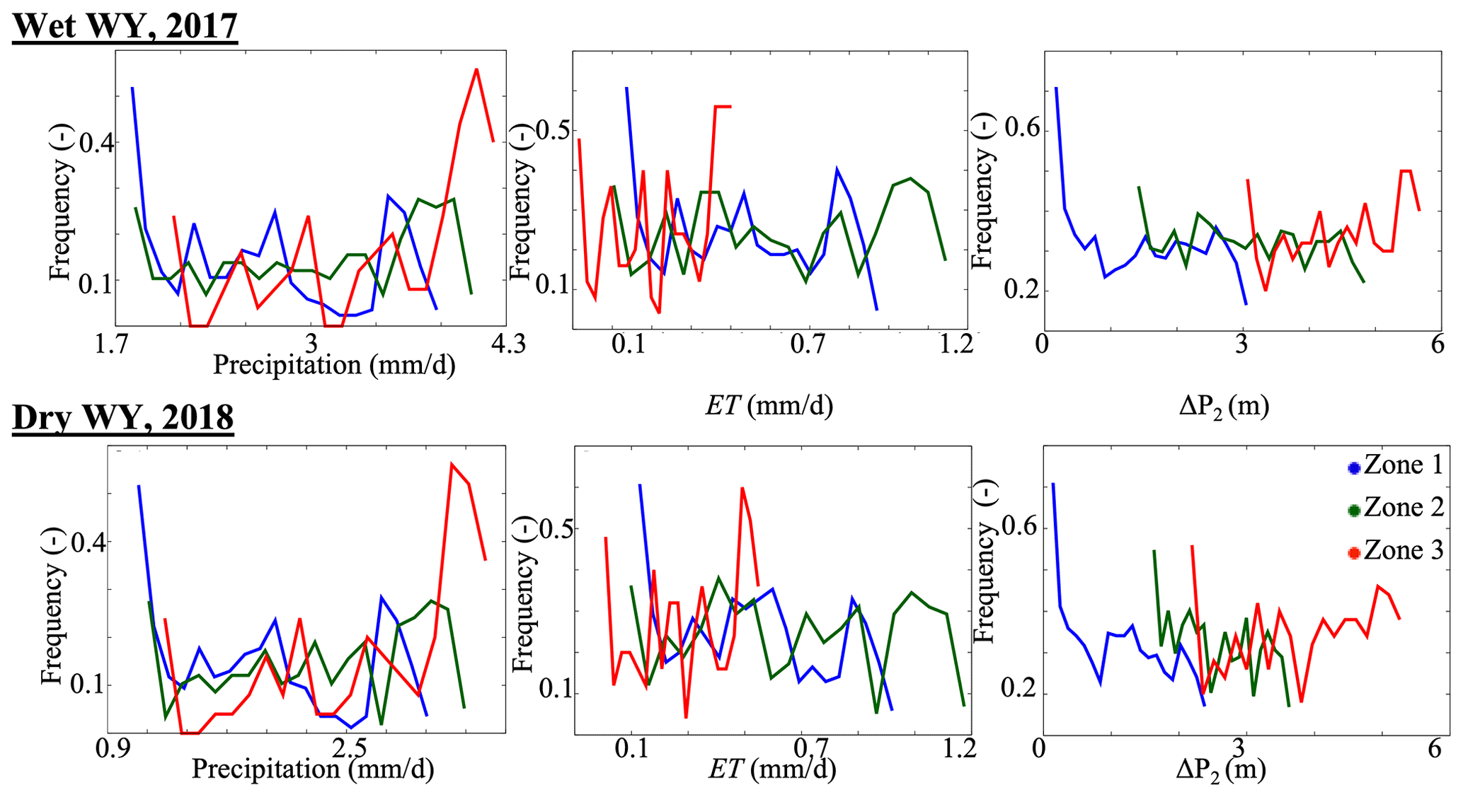
Figure 10Frequency distributions of hillslope annual average daily rates of precipitation and evapotranspiration (ET), and the hillslope seasonal changes in groundwater levels (ΔP2), in 2017 (wet WY) and 2018 (dry WY) of the three zones derived from the WY 2015 ΔP1.
4.2 Similarities in hydrologic responses to wet and dry conditions
According to McDonnell and Woods (2004) and Wagener et al., (2007), any classification should be able to predict the dynamics of hillslopes. We test the ability of the ΔP1 clustering to predict the dynamics of hillslopes in wet and dry conditions. A possible limitation of a clustering based on a hydrologic process is that the latter may be linked to the conditions of the selected year. Hydrologic responses are, by essence, nonlinear and may strongly change from year to year. In addition, compared to the intrinsic characteristics of the hillslope (elevation, topographic index, and land cover), which are only variable if long periods of time are considered, the scale at which hydrologic processes change is much shorter. Therefore, a clustering based on a hydrologic process may be time-dependent. We previously quantified ΔP1 using an average WY. In this section, we compare the response of each zone to dry and wet conditions. We extend our simulation from the WY 2015 to include the WYs 2016, 2017, and 2018, then, we analyze WYs 2017 and 2018. This four-year simulation covers a relatively wet (2017) and dry (2018) WY. The annual average precipitation in 2017 was ∼ 15 % higher than the annual average precipitation in 2015. After this wet WY, the watershed is characterized by a dry climate in 2018, with average precipitation almost 50 % below the normal conditions. Figure 10 shows the distributions of hillslope annual average values of precipitation and ET, the hillslope ΔP2 associated with the defined ΔP1 zones, and for both the wet WY 2017 and the dry WY 2018. We have selected the key variables describing the hydroclimate (precipitation), land surface processes (ET), and subsurface hydrodynamics (ΔP2).
At first glance, for both dry and wet years and selected processes, all zones remain distinct. Zone 1 with hillslopes with low ΔP1, located in low elevation, remains with low precipitation and high ET through both wet and dry years. Zone 3 describing hillslopes with high ΔP1, has the highest precipitation in the area during both the wet and dry years. The hillslopes of Zone 2, located in mid-elevation, have most of their hydrologic dynamics in between those of Zone 1 and 3, except their ET, which is the highest in the area due to the presence of forests. Our results show that although we defined hillslope clustering based on a hydrologic process during an average WY, our clustering approach can predict the similarity of the dynamics of these hillslopes in wet and dry conditions. The ΔP1 clustering is, therefore, robust in predicting similarity in hydrologic responses under both wet and dry conditions.
In this study, we use seasonal changes in groundwater levels – termed ΔP1 – to identify and categorize similar hillslopes. ΔP1 is an important variable controlled by many hydrologic processes, including land surface processes and hydroclimatic. We defined three zones based on their similarity in ΔP1. For a test case site in the East River watershed, Zone 1 characterizes hillslopes with low ΔP1; these hillslopes are mostly located in low elevation areas, their main land cover is grassland, and their ET is high because their WTDs are shallow. Zone 3, on the opposite of Zone 1, is located in high elevation areas and has high ΔP1; the hydroclimate leads to high snow accumulation and low ET. Hillslopes of Zone 3 are mostly bare soil. Zone 2 is in between these two zones and most of the hillslopes of this zone are covered by forests.
We tested the performance of the proposed ΔP1 clustering by comparing it with other existing clustering approaches. This was based on elevation, land cover, aridity index, a topographic wetting index, and three clustering approaches based on machine learning, which uses multiple data layers including model inputs and outputs. Our results show that the ΔP1 clustering is robust as it reasonably identifies and categorizes hillslopes with similar elevation, land cover, hydroclimate characteristics, land surface processes (ET and SWE), and subsurface hydrodynamics (WTD, soil moisture, and ΔP1). In general, the other clustering approaches are good in identifying similarity in a single characteristic related to the variable determining the clustering. Our work also demonstrates that a clustering using machine learning, either based on top-down (inputs) or bottom-up (outputs), performs well. Nevertheless, these clustering approaches, like the ΔP1, require multiple data sets, each one with its own associated uncertainty. We further demonstrate the robustness of the proposed ΔP1 clustering by testing its ability to predict hillslope responses to wet and dry hydrologic conditions. The ΔP1 values are derived from a model and could be a limitation for sites where simulated outputs are unavailable or the spatio-temporal resolution of groundwater observations are limited. In addition, one of the main limitations of the proposed clustering is that due to the disconnection between land surface processes and structures and the subsurface dynamics in some regions, this clustering approach cannot be used in these conditions.
Future studies could aim to identify similar hillslopes using ΔP1 and sophisticated machine learning approaches or optimization procedures. Our results are limited to one catchment, which has snow-dominated hydrology. Future studies could expand the comparison shown here to other watersheds to include additional clustering approaches and for different hydroclimate and durations of time (for example, sub-annual or multi-annual clustering).
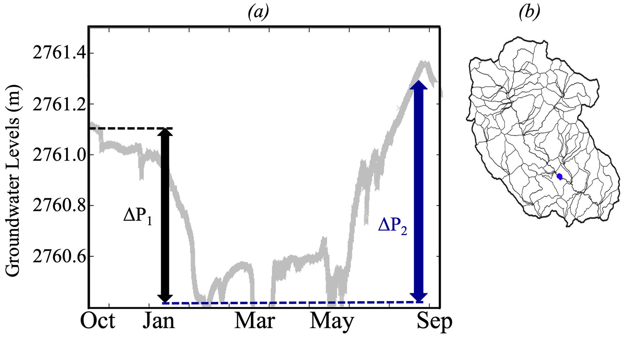
Figure A1(a) Measured groundwater levels in WY2016 at a station located in blue in (b).
The ParFlow-CLM integrated hydrologic model can be found here: https://parflow.org/#download (ParFlow, 2022). Data supporting the findings of this study are freely available on ESS-DIVE: https://ess-dive.lbl.gov (ESS-DIVE, 2022: Wainwright et al., 2022; https://doi.org/10.15485/1602034: Falco et al., 2020; https://doi.org/10.15485/1617203: Goulden et al., 2020).
FZM was responsible for conceptualizing the study, undertaking the formal analysis, writing and preparing the original draft of the paper, and reviewing and editing the paper. HW was responsible for conceptualizing the study, undertaking the formal analysis, writing and preparing the original draft of the paper, and reviewing and editing the paper. PJDF was responsible for conceptualizing the study, writing and preparing the original draft of the paper, and reviewing and editing the paper. ERSW was responsible for conceptualizing the study, undertaking the formal analysis, writing and preparing the original draft of the paper, and reviewing and editing the paper.
The contact author has declared that neither they nor their co-authors have any competing interests.
Publisher's note: Copernicus Publications remains neutral with regard to jurisdictional claims in published maps and institutional affiliations.
This material is based on work supported as part of the Watershed Function Scientific Focus Area funded by the US Department of Energy, Office of Science, Office of Biological and Environmental Research under grant no. DE-AC02-05 CH11231.
This research has been supported by the US Department of Energy (grant no. DE-AC02-05 CH11231).
This paper was edited by Hilary McMillan and reviewed by two anonymous referees.
Andréassian, V., Lerat, J., Le Moine, N., and Perrin, C.: Neighbors: Nature's own hydrological models, J. Hydrol., 414–415, 49–58, https://doi.org/10.1016/j.jhydrol.2011.10.007, 2012.
Aryal, S. K., O'Loughlin, E. M., and Mein, R. G.: A similarity approach to predict landscape saturation in catchments, Water Resour. Res., 38, 26-1-26–16, https://doi.org/10.1029/2001WR000864, 2002.
Berghuijs, W. R., Sivapalan, M., Woods, R. A., and Savenije, H. H. G.: Patterns of similarity of seasonal water balances: A window into streamflow variability over a range of time scales, Water Resour. Res., 50, 5638–5661, https://doi.org/10.1002/2014WR015692, 2014.
Berne, A., Uijlenhoet, R., and Troch, P. A.: Similarity analysis of subsurface flow response of hillslopes with complex geometry, Water Resour. Res., 41, W09410, https://doi.org/10.1029/2004WR003629, 2005.
Beven, K. J.: Uniqueness of place and process representations in hydrological modelling, Hydrol. Earth Syst. Sci., 4, 203–213, https://doi.org/10.5194/hess-4-203-2000, 2000.
Beven, K. J. and Kirkby, M. J.: A physically based, variable contributing area model of basin hydrology/Un modèle à base physique de zone d'appel variable de l'hydrologie du bassin versant, Hydrol. Sci. B., 24, 43–69, https://doi.org/10.1080/02626667909491834, 1979.
Bormann, H.: Towards a hydrologically motivated soil texture classification, Geoderma, 157, 142–153, https://doi.org/10.1016/j.geoderma.2010.04.005, 2010.
Bosch, J. M. and Hewlett, J. D.: A review of catchment experiments to determine the effect of vegetation changes on water yield and evapotranspiration, J. Hydrol., 55, 3–23, https://doi.org/10.1016/0022-1694(82)90117-2, 1982.
Brown, A. E., Zhang, L., McMahon, T. A., Western, A. W., and Vertessy, R. A.: A review of paired catchment studies for determining changes in water yield resulting from alterations in vegetation, J. Hydrol., 310, 28–61, https://doi.org/10.1016/j.jhydrol.2004.12.010, 2005.
Brunner, P. and Simmons, C. T.: HydroGeoSphere: A Fully Integrated, Physically Based Hydrological Model, Groundwater, 50, 170–176, https://doi.org/10.1111/j.1745-6584.2011.00882.x, 2012.
Carrillo, G., Troch, P. A., Sivapalan, M., Wagener, T., Harman, C., and Sawicz, K.: Catchment classification: hydrological analysis of catchment behavior through process-based modeling along a climate gradient, Hydrol. Earth Syst. Sci., 15, 3411–3430, https://doi.org/10.5194/hess-15-3411-2011, 2011.
Carroll, R. W. H., Bearup, L. A., Brown, W., Dong, W., Bill, M., and Willlams, K. H.: Factors controlling seasonal groundwater and solute flux from snow-dominated basins, Hydrol. Process., 32, 2187–2202, https://doi.org/10.1002/hyp.13151, 2018.
CGIAR-CSI: Global Aridity Index and Potential Evapotranspiration Climate Database v2, https://cgiarcsi.community/2019/01/24/global-aridity-index-and-potential-evapotranspiration-climate-database-v2/ (last access: 22 August 2020) 2019.
Chadwick, K. D., Brodrick, P. G., Grant, K., Goulden, T., Henderson, A., Falco, N., Wainwright, H., Williams, K. H., Bill, M., Breckheimer, I., Brodie, E. L., Steltzer, H., Williams, C. F. R., Blonder, B., Chen, J., Dafflon, B., Damerow, J., Hancher, M., Khurram, A., Lamb, J., Lawrence, C. R., McCormick, M., Musinsky, J., Pierce, S., Polussa, A., Hastings Porro, M., Scott, A., Singh, H. W., Sorensen, P. O., Varadharajan, C., Whitney, B., and Maher, K.: Integrating airborne remote sensing and field campaigns for ecology and earth system science, Methods Ecol. Evol., 11, 1492–1508, https://doi.org/10.1111/2041-210x.13463, 2020.
Chaney, N. W., Van Huijgevoort, M. H. J., Shevliakova, E., Malyshev, S., Milly, P. C. D., Gauthier, P. P. G., and Sulman, B. N.: Harnessing big data to rethink land heterogeneity in Earth system models, Hydrol. Earth Syst. Sci., 22, 3311–3330, https://doi.org/10.5194/hess-22-3311-2018, 2018.
Condon, L. E., Maxwell, R. M., and Gangopadhyay, S.: The impact of subsurface conceptualization on land energy fluxes, Adv. Water Resour., 60, 188–203, https://doi.org/10.1016/j.advwatres.2013.08.001, 2013.
Coon, E. T., David Moulton, J., and Painter, S. L.: Managing complexity in simulations of land surface and near-surface processes, Environ. Modell. Softw., 78, 134–149, https://doi.org/10.1016/j.envsoft.2015.12.017, 2016.
Cosgrove, B. A., Lohmann, D., Mitchell, K. E., Houser, P. R., Wood, E. F., Schaake, J. C., Robock, A., Marshall, C., Sheffield, J., Duan, Q., Luo, L., Higgins, R. W., Pinker, R. T., Tarpley, J. D., and Meng, J.: Real-time and retrospective forcing in the North American Land Data Assimilation System (NLDAS) project, J. Geophys. Res.-Atmos., 108, 8842, https://doi.org/10.1029/2002JD003118, 2003.
Dai, Y., Zeng, X., Dickinson, R. E., Baker, I., Bonan, G. B., Bosilovich, M. G., Denning, A. S., Dirmeyer, P. A., Houser, P. R., Niu, G., Oleson, K. W., Schlosser, C. A., and Yang, Z.-L.: The Common Land Model, B. Am. Meteorol. Soc., 84, 1013–1024, https://doi.org/10.1175/BAMS-84-8-1013, 2003.
Daly, C., Halbleib, M., Smith, J. I., Gibson, W. P., Doggett, M. K., Taylor, G. H., Curtis, J., and Pasteris, P. P.: Physiographically sensitive mapping of climatological temperature and precipitation across the conterminous United States, Int. J. Climatol., 28, 2031–2064, https://doi.org/10.1002/joc.1688, 2008.
Devadoss, J., Falco, N., Dafflon, B., Wu, Y., Franklin, M., Hermes, A., Hinckley, E.-L. S., and Wainwright, H.: Remote Sensing-Informed Zonation for Understanding Snow, Plant and Soil Moisture Dynamics within a Mountain Ecosystem, Remote Sens.-Basel, 12, 2733, https://doi.org/10.3390/rs12172733, 2020.
ESS-DIVE: About ESS-DIVE, ESS-DIVE, https://ess-dive.lbl.gov, last access: 5 July 2022.
Falco, N., Balde, A., Breckheimer, I., Brodie, E., Brodrick, P. G., Chadwick, K. D., Chen, J., Dafflon, B., Henderson, A., Lamb, J., Maher, K., Kueppers, L., Steltzer, H., Wainwright, H., Williams, K., and Hubbard, S. S.: Plant species distribution within the Upper Colorado River Basin estimated by using hyperspectral and lidar airborne data, Watershed Function SFA, ESS-DIVE repository [data set], https://doi.org/10.15485/1602034, 2020.
Fan, Y., Clark, M., Lawrence, D. M., Swenson, S., Band, L. E., Brantley, S. L., Brooks, P. D., Dietrich, W. E., Flores, A., Grant, G., Kirchner, J. W., Mackay, D. S., McDonnell, J. J., Milly, P. C. D., Sullivan, P. L., Tague, C., Ajami, H., Chaney, N., Hartmann, A., Hazenberg, P., McNamara, J., Pelletier, J., Perket, J., Rouholahnejad‐Freund, E., Wagener, T., Zeng, X., Beighley, E., Buzan, J., Huang, M., Livneh, B., Mohanty, B. P., Nijssen, B., Safeeq, M., Shen, C., Verseveld, W. van, Volk, J., and Yamazaki, D.: Hillslope Hydrology in Global Change Research and Earth System Modeling, Water Resour. Res., 55, 1737–1772, https://doi.org/10.1029/2018WR023903, 2019.
Ferguson, I. M. and Maxwell, R. M.: Role of groundwater in watershed response and land surface feedbacks under climate change, Water Resour. Res., 46, W00F02, https://doi.org/10.1029/2009WR008616, 2010.
Foster, L. M. and Maxwell, R. M.: Sensitivity analysis of hydraulic conductivity and Manning's n parameters lead to new method to scale effective hydraulic conductivity across model resolutions, Hydrol. Process., 33, 332–349, https://doi.org/10.1002/hyp.13327, 2019.
Goulden, T., Hass, B., Brodie, E., Chadwick, K. D., Falco, N., Maher, K., Wainwright, H., and Williams, K.: NEON AOP Survey of Upper East River CO Watersheds: LAZ Files, LiDAR Surface Elevation, Terrain Elevation, and Canopy Height Rasters, Watershed Function SFA, ESS-DIVE repository [data set], https://doi.org/10.15485/1617203, 2020.
Grabs, T., Seibert, J., Bishop, K., and Laudon, H.: Modeling spatial patterns of saturated areas: A comparison of the topographic wetness index and a dynamic distributed model, J. Hydrol., 373, 15–23, https://doi.org/10.1016/j.jhydrol.2009.03.031, 2009.
Harman, C. and Sivapalan, M.: A similarity framework to assess controls on shallow subsurface flow dynamics in hillslopes, Water Resour. Res., 45, W01417, https://doi.org/10.1029/2008WR007067, 2009.
Hjerdt, K. N., McDonnell, J. J., Seibert, J., and Rodhe, A.: A new topographic index to quantify downslope controls on local drainage, Water Resour. Res., 40, W05602, https://doi.org/10.1029/2004WR003130, 2004.
Hubbard, S. S., Williams, K. H., Agarwal, D., Banfield, J., Beller, H., Bouskill, N., Brodie, E., Carroll, R., Dafflon, B., Dwivedi, D., Falco, N., Faybishenko, B., Maxwell, R., Nico, P., Steefel, C., Steltzer, H., Tokunaga, T., Tran, P. A., Wainwright, H., and Varadharajan, C.: The East River, Colorado, Watershed: A Mountainous Community Testbed for Improving Predictive Understanding of Multiscale Hydrological–Biogeochemical Dynamics, Vadose Zone J., 17, 180061, https://doi.org/10.2136/vzj2018.03.0061, 2018.
IGBP: Global plant database published – IGBP [text], http://www.igbp.net/news/news/news/globalplantdatabasepublished.5.1b8ae20512db692f2a6800014762.html, last access: 17 October 2018.
Jefferson, J. L., Gilbert, J. M., Constantine, P. G., and Maxwell, R. M.: Active subspaces for sensitivity analysis and dimension reduction of an integrated hydrologic model, Comput. Geosci., 83, 127–138, https://doi.org/10.1016/j.cageo.2015.07.001, 2015.
Kassambara, A.: Practical guide to cluster analysis in R: Unsupervised machine learning, in: Vol. 1, Sthda, ISBN 13 978-1542462709, 2017.
Loritz, R., Kleidon, A., Jackisch, C., Westhoff, M., Ehret, U., Gupta, H., and Zehe, E.: A topographic index explaining hydrological similarity by accounting for the joint controls of runoff formation, Hydrol. Earth Syst. Sci., 23, 3807–3821, https://doi.org/10.5194/hess-23-3807-2019, 2019.
Lyon, S. W. and Troch, P. A.: Hillslope subsurface flow similarity: Real-world tests of the hillslope Péclet number, Water Resour. Res., 43, W07450, https://doi.org/10.1029/2006WR005323, 2007.
Lyon, S. W. and Troch, P. A.: Development and application of a catchment similarity index for subsurface flow, Water Resour. Res., 46, W03511, https://doi.org/10.1029/2009WR008500, 2010.
Maina, F. Z. and Siirila-Woodburn, E. R.: The Role of Subsurface Flow on Evapotranspiration: A Global Sensitivity Analysis, Water Resour. Res., 56, e2019WR026612, https://doi.org/10.1029/2019WR026612, 2020.
Maina, F. Z., Siirila-Woodburn, E. R., Newcomer, M., Xu, Z., and Steefel, C.: Determining the impact of a severe dry to wet transition on watershed hydrodynamics in California, USA with an integrated hydrologic model, J. Hydrol., 580, 124358, https://doi.org/10.1016/j.jhydrol.2019.124358, 2020.
Maina, F. Z., Siirila-Woodburn, E. R., and Dennedy-Frank, P. J.: Assessing the impacts of hydrodynamic parameter uncertainties on simulated evapotranspiration in a mountainous watershed, J. Hydrol., 608, 127620, https://doi.org/10.1016/j.jhydrol.2022.127620, 2022.
Maxwell, R. M.: A terrain-following grid transform and preconditioner for parallel, large-scale, integrated hydrologic modeling, Adv. Water Resour., 53, 109–117, https://doi.org/10.1016/j.advwatres.2012.10.001, 2013.
Maxwell, R. M. and Condon, L. E.: Connections between groundwater flow and transpiration partitioning, Science, 353, 377–380, https://doi.org/10.1126/science.aaf7891, 2016.
Maxwell, R. M. and Miller, N. L.: Development of a Coupled Land Surface and Groundwater Model, J. Hydrometeorol., 6, 233–247, https://doi.org/10.1175/JHM422.1, 2005.
McDonnell, J. J. and Woods, R.: On the need for catchment classification, J. Hydrol., 299, 2–3, https://doi.org/10.1016/j.jhydrol.2004.09.003, 2004.
Noël, P., Rousseau, A. N., Paniconi, C., and Nadeau, D. F.: Algorithm for Delineating and Extracting Hillslopes and Hillslope Width Functions from Gridded Elevation Data, J. Hydrol. Eng., 19, 366–374, https://doi.org/10.1061/(ASCE)HE.1943-5584.0000783, 2014.
Oudin, L., Kay, A., Andréassian, V., and Perrin, C.: Are seemingly physically similar catchments truly hydrologically similar?, Water Resour. Res., 46, W11558, https://doi.org/10.1029/2009WR008887, 2010.
ParFlow: ParFlow hydrologic model, ParFlow, https://parflow.org/#download, last access: 5 July 2022.
Pribulick, C. E., Foster, L. M., Bearup, L. A., Navarre-Sitchler, A. K., Williams, K. H., Carroll, R. W. H., and Maxwell, R. M.: Contrasting the hydrologic response due to land cover and climate change in a mountain headwaters system, Ecohydrology, 9, 1431–1438, https://doi.org/10.1002/eco.1779, 2016.
Rahman, M., Sulis, M., and Kollet, S. J.: Evaluating the dual-boundary forcing concept in subsurface–land surface interactions of the hydrological cycle, Hydrol. Process., 30, 1563–1573, https://doi.org/10.1002/hyp.10702, 2016.
Richards, L. A.: Capillary conduction of liquids through porous medium, J. Appl. Phys., 1, 318–333, https://doi.org/10.1063/1.1745010, 1931.
Ryken, A., Bearup, L. A., Jefferson, J. L., Constantine, P., and Maxwell, R. M.: Sensitivity and model reduction of simulated snow processes: Contrasting observational and parameter uncertainty to improve prediction, Adv. Water Resour., 135, 103473, https://doi.org/10.1016/j.advwatres.2019.103473, 2020.
Sawicz, K., Wagener, T., Sivapalan, M., Troch, P. A., and Carrillo, G.: Catchment classification: empirical analysis of hydrologic similarity based on catchment function in the eastern USA, Hydrol. Earth Syst. Sci., 15, 2895–2911, https://doi.org/10.5194/hess-15-2895-2011, 2011.
Schwanghart, W. and Scherler, D.: Short Communication: TopoToolbox 2 – MATLAB-based software for topographic analysis and modeling in Earth surface sciences, Earth Surf. Dynam., 2, 1–7, https://doi.org/10.5194/esurf-2-1-2014, 2014.
Sivapalan, M., Takeuchi, K., Franks, S. W., Gupta, V. K., Karambiri, H., Lakshmi, V., Liang, X., McDonnell, J. J., Mendiondo, E. M., O'Connell, P. E., Oki, T., Pomeroy, J. W., Schertzer, D., Uhlenbrook, S., and Zehe, E.: IAHS Decade on Predictions in Ungauged Basins (PUB), 2003–2012: Shaping an exciting future for the hydrological sciences, Hydrolog. Sci. J., 48, 857–880, https://doi.org/10.1623/hysj.48.6.857.51421, 2003.
van Genuchten, M. T.: A Closed-form Equation for Predicting the Hydraulic Conductivity of Unsaturated Soils1, Soil Sci. Soc. Am. J., 44, 892, https://doi.org/10.2136/sssaj1980.03615995004400050002x, 1980.
Wagener, T., Sivapalan, M., Troch, P., and Woods, R.: CatchmentClassification and Hydrologic Similarity, Geography Compass, 1, 901–931, https://doi.org/10.1111/j.1749-8198.2007.00039.x, 2007.
Wainwright, H. M., Uhlemann, S., Franklin, M., Falco, N., Bouskill, N. J., Newcomer, M. E., Dafflon, B., Siirila-Woodburn, E. R., Minsley, B. J., Williams, K. H., and Hubbard, S. S.: Watershed zonation through hillslope clustering for tractably quantifying above- and below-ground watershed heterogeneity and functions, Hydrol. Earth Syst. Sci., 26, 429–444, https://doi.org/10.5194/hess-26-429-2022, 2022.
Winnick, M. J., Carroll, R. W. H., Williams, K. H., Maxwell, R. M., Dong, W., and Maher, K.: Snowmelt controls on concentration-discharge relationships and the balance of oxidative and acid-base weathering fluxes in an alpine catchment, East River, Colorado, Water Resour. Res., 53, 2507–2523, https://doi.org/10.1002/2016WR019724, 2017.