the Creative Commons Attribution 4.0 License.
the Creative Commons Attribution 4.0 License.
 | 15 Jul 2022
Multi-scale temporal analysis of evaporation on a saline lake in the Atacama Desert
Felipe Lobos-Roco
Oscar Hartogensis
Francisco Suárez
Ariadna Huerta-Viso
Imme Benedict
Alberto de la Fuente
Jordi Vilà-Guerau de Arellano
We investigate how evaporation changes depending on the scales in the Altiplano region of the Atacama Desert. More specifically, we focus on the temporal evolution from the climatological to the sub-diurnal scales on a high-altitude saline lake ecosystem. We analyze the evaporation trends over 70 years (1950–2020) at a high-spatial resolution. The method is based on the downscaling of 30 km ERA5 reanalysis data at hourly resolution to 0.1 km spatial resolution data, using artificial neural networks to analyze the main drivers of evaporation. To this end, we use the Penman open-water evaporation equation, modified to compensate for the energy balance non-closure and the ice cover formation on the lake during the night. Our estimation of the hourly climatology of evaporation shows a consistent agreement with eddy-covariance (EC) measurements and reveals that evaporation is controlled by different drivers depending on the time scale. At the sub-diurnal scale, mechanical turbulence is the primary driver of evaporation, and at this scale, it is not radiation-limited. At the seasonal scale, more than 70 % of the evaporation variability is explained by the radiative contribution term. At the same scale, and using a large-scale moisture tracking model, we identify the main sources of moisture to the Chilean Altiplano. In all cases, our regime of precipitation is controlled by large-scale weather patterns closely linked to climatological fluctuations. Moreover, seasonal evaporation significantly influences the saline lake surface spatial changes. From an interannual scale perspective, evaporation increased by 2.1 mm yr−1 during the entire study period, according to global temperature increases. Finally, we find that yearly evaporation depends on the El Niño–Southern Oscillation (ENSO), where warm and cool ENSO phases are associated with higher evaporation and precipitation rates, respectively. Our results show that warm ENSO phases increase evaporation rates by 15 %, whereas cold phases decrease it by 2 %.
- Article
(9341 KB) - Full-text XML
- BibTeX
- EndNote


In arid regions, evaporation is one of the most important components in the water cycle since potential evaporation is typically 1 order of magnitude larger than precipitation (Lictevout et al., 2013; Houston, 2006). Investigating evaporation in these regions is challenging due to the lack of observations, the landscape complexity, and the poor representation in hydrometeorological models. The climate/large-scale atmospheric circulation and spatially localized zones affect water availability (Lobos-Roco et al., 2021). At a local level in the Atacama Desert, evaporation occurs (Houston, 2006): (i) in rivers and the adjacent riparian zones; (ii) in marshlands, where localized groundwater springs support vegetation growth and sometimes contribute to the formation of shallow terminal lakes (de la Fuente and Meruane, 2017; Jayne et al., 2016), which generally occurs in the Andes Mountains; (iii) in salt flats or playas, which are the result of more extensive groundwater discharge in endorheic basins (de la Fuente, 2014; de la Fuente and Meruane, 2017; Scheihing et al., 2017); and (iv) in bare soils where the water table is shallow (Rosen, 1994; Johnson et al., 2010; Uribe et al., 2015; Blin et al., 2022). The Chilean Altiplano is an arid zone where water evaporates from spatially localized environments, removing water from the basin. The Altiplano region has a unique environmental, economic and social value due to its location within the Atacama Desert, where groundwater fed by a short, annual rainy period provides the main source of water for northern Chile. A reliable understanding of the processes that govern evaporation in this region is essential for three main reasons (Suárez et al., 2020): (i) water resource management because a correct quantification of these fluxes enhances the performance of water balance models and improves the estimation of the basin's water recharge, (ii) terrestrial and aquatic ecosystems that sustain the native flora and fauna of this region, and (iii) sustainable agricultural and mining production in terms of minimizing environmental impacts and maximizing water use. Within the Altiplano, the Salar del Huasco (SDH) basin is chosen for studying evaporation due to the perennial terminal saline lake where nonlocal atmospheric processes occur (Suárez et al., 2020; Lobos-Roco et al., 2021). This lake, untouched by human activities (Uribe et al., 2015), has been well-studied in recent years. These studies have focused on quantifying and understanding evaporation (Voigt et al., 2021; Suárez et al., 2020; Lobos-Roco et al., 2021, 2022) for use in water resource management models (Uribe et al., 2015; Blin et al., 2022). Thus, there are many comprehensive datasets of surface and upper-atmospheric observations for the SDH basin that can be used to relate large-scale atmospheric phenomena with small-scale processes and, in turn, to advance our understanding of evaporation and its use for water resource conservation.
Synoptic and regional circulation over the Altiplano region, responsible for moisture transport and precipitation, has been studied by Rutllant et al. (2003), Falvey and Garreaud (2005) and Böhm et al. (2020). These studies investigated how large-scale atmospheric phenomena influenced by the Pacific Ocean, steep Andean topography and the Amazon basin organize circulations at different scales. These atmospheric circulations are the main contributors of moisture in the region. Two marked phases characterize the principal synoptic atmospheric circulation over the Altiplano region. The first phase occurs during the summer season (December to March). It is characterized by westward winds from the Amazon basin, which transport a significant amount of moisture over the Altiplano (Falvey and Garreaud, 2005). This moisture transport is highly variable from year to year, and it is responsible for convective rains that occur in the region. In the second phase, dry air from the free troposphere above the Pacific Ocean is transported to the Altiplano region in the Andes (Rutllant et al., 2003) and occurs from April to November. This dry-air transport results from the thermal differences between the western slope of the Atacama Desert and the Pacific Ocean (Lobos-Roco et al., 2021). Other studies have reported the effects of the El Niño–Southern Oscillation (ENSO) and the Pacific Decadal Oscillation (PDO) on precipitation patterns. Böhm et al. (2020) studied the integrated water vapor (IWV) variability and its relationship with the ENSO phenomenon in the Atacama Desert during the 20th century. Their results revealed that cool ENSO phases (associated with the La Niña ENSO phenomenon) yield greater IWV variability which favors more extreme wet conditions during the austral summer in the Altiplano region. Garreaud et al. (2003) analyzed the climatic conditions from inter-seasonal to glacial–interglacial timescales. Researchers found that mean zonal airflow over the region modulates interannual changes in the climatic condition over the Altiplano. This airflow responds to sea surface temperature variability in the tropical section of the Pacific Ocean. Likewise, several studies have pointed out the remarkable control that cool ENSO phases exert over the precipitation in the Altiplano (Aceituno, 1988; Vuille et al., 2000; Garreaud and Aceituno, 2001). This control shows that cool ENSO phases yield wetter rainy seasons, whereas warm ENSO phases (El Niño) result in drier rainy seasons (Garreaud and Aceituno, 2001). The ENSO influence on climatic factors such as precipitation implies that evaporation, as a temperature-dependent process, might also be affected by this phenomenon (Houston, 2006).
The spatiotemporal evolution of evaporation has also been investigated in the Altiplano region of the Atacama Desert. These studies aimed to understand the complex diurnal land–atmosphere turbulent transport over different surfaces (Kampf et al., 2005; de la Fuente and Meruane, 2017; Lobos-Roco et al., 2021), characterizing the larger-scale influence on the local evaporation (Suárez et al., 2020; Lobos-Roco et al., 2021), or simply to assess daily evaporation from bare soils in order to develop relationships that can be used to relate evaporation with the water-table depth (Johnson et al., 2010). These investigations mainly focused on short-term field experiments based on either daily measurements (Kampf et al., 2005; Suárez et al., 2020) or applied models used to predict potential evaporation (de la Fuente and Meruane, 2017). Even with these studies, long-term evaporation observations at a local scale are still lacking, especially when trying to construct conceptual models that can be used for water resource management. For instance, Uribe et al. (2015) developed a hydrological model in the SDH region where evaporation was estimated using information from evaporation pans, and regional vertical gradients in evaporation were seen as a function of elevation. Blin et al. (2022) developed a groundwater model for SDH. This groundwater model, which was used to assess climate change impacts on the SDH basin, utilized the hydrological model constructed by Uribe et al. (2015) to determine aquifer recharge and to estimate the evaporation discharge to the atmosphere. Unfortunately, these models overlook the influence of the nonlocal atmospheric processes, such as the entrainment and advection of heat, moisture and momentum, on evaporation rates (Suárez et al., 2020; Lobos-Roco et al., 2021, 2022). Attempting to rectify this oversight, recent experimental field campaigns have been carried out in the Altiplano area of the Atacama Desert (Suárez et al., 2020). However, the lack of reliable long-term actual evaporation estimates still limits our complete understanding of the climate change impacts on water availability in these arid areas. Moreover, there are no studies that aim to investigate the myriad of links between these temporal short- and large-scale studies. Thus, our objective is to understand seasonal and interannual evaporation variability by examining how surface energy partitioning, turbulence and moisture supply affect seasonal changes in evaporation. In this way, we aim to bridge this cross-scale knowledge gap which will help to address water availability in the Atacama Desert.
In this study, we applied climatologically robust, downscaled reanalysis data to the saline lake of SDH. Although we focused on one particular saline lake, this kind of surface represents the main evaporation pathway of the Altiplano region (Houston, 2006). We hypothesized that the evaporation of the saline lake can be represented using an adapted version of the Penman (1948) equation. Confirmation of this hypothesis enables us to extend the adapted Penman model to the entire climatological period (1950–2020) and to investigate evaporation fluctuations and their drivers at seasonal and interannual scales.
2.1 Study area
Our study area is located in the SDH basin (1462 km2), with its highest point at 5200 m above sea level (m a.s.l.), and its lowest point at 3790 m a.s.l. (Uribe et al., 2015). This endorheic basin is located to the west of the Andes, 135 km inland from the Pacific Ocean, and is subject to an intense and recurrent afternoon atmospheric flow from the ocean that transports relatively cold and humid air into the Altiplano (Lobos-Roco et al., 2021). The basin is also affected by the moist atmospheric flow coming from the east, which is responsible for a marked rainy season during the austral summer, where short convective storms are the main source of aquifer recharge (Blin et al., 2022). Since evaporation occurs where there is available water, our research focused on the basin's sink, which is a wetland in SDH (de la Fuente et al., 2021). Specifically, our attention is placed on the saline lake of SDH (20.2∘ S, 68.8∘ W 3790 m a.s.l.), which is a perennial water body surrounded by salt crusts, zones with native vegetation patches and zones with bare soils (Fig. 1). This terminal lake shows significant seasonal changes in its surface, ranging between ∼0.5 to 5 km2, with a measured depth of ∼15 cm (Lobos-Roco et al., 2021). These types of groundwater-fed wetlands are commonly found in the Altiplano region (Kampf et al., 2005), and result in unique ecological habitats for endemic flora and fauna (Dorador et al., 2013).
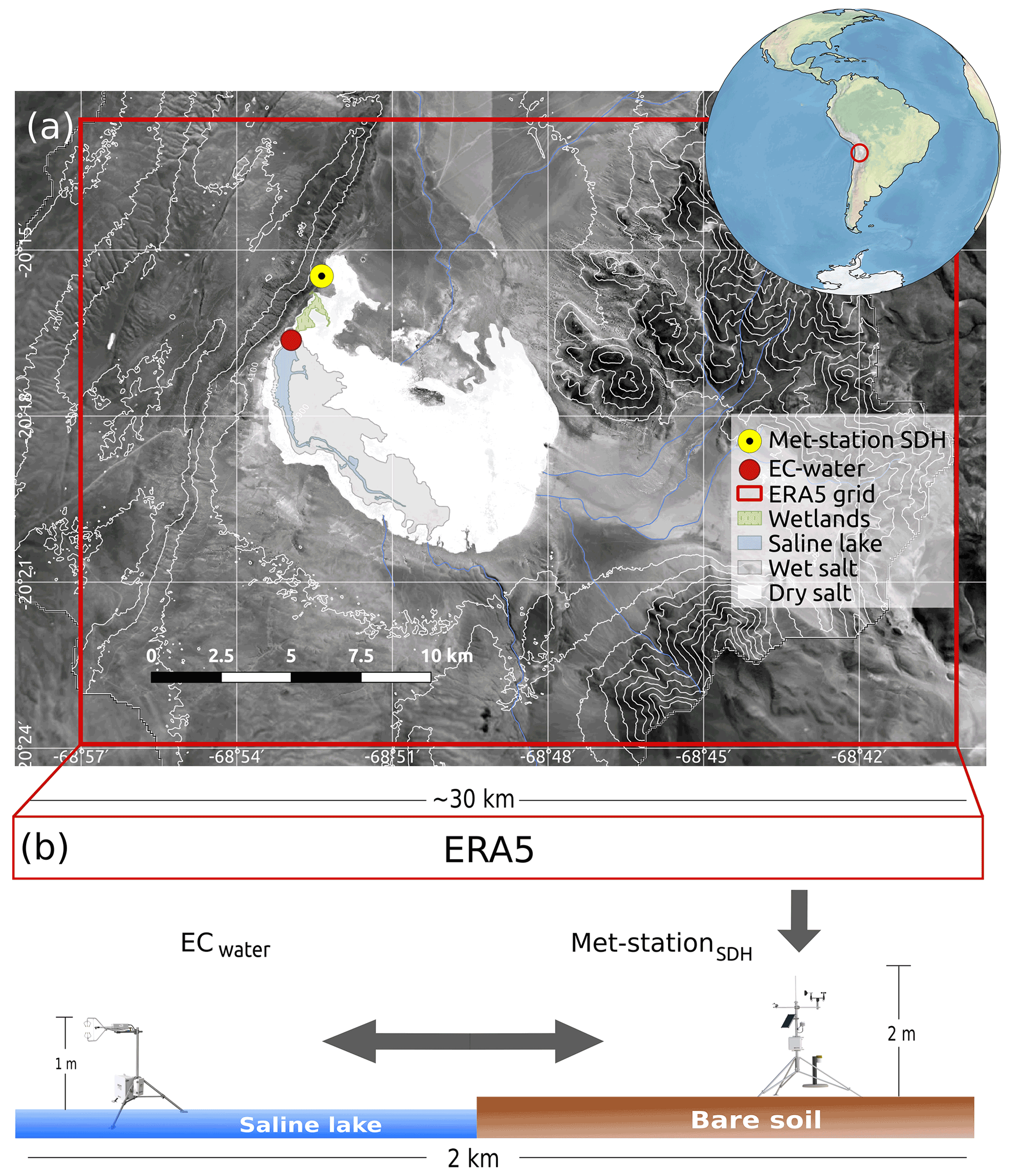
Figure 1(a) Salar del Huasco (SDH) saline lake and location of the meteorological station and the eddy-covariance (EC) system used in this investigation. The red square shows an approximated grid size of the ERA5 reanalysis data. (b) Schematic cross-section of the meteorological downscaling from larger to smaller spatial scales. It contains modified Copernicus Sentinel data processed by Sentinel Hub, ESA.
2.2 Data acquisition
This study combines data from different sources including observations, modeling reanalysis data and remote sensing datasets. Table 1 summarizes the datasets, variables, frequency, spatial resolution and sources employed in this research.
Suárez et al., 2020Lobos-Roco et al., 2020Hersbach et al. (2020)Dee et al. (2011)de la Fuente et al. (2021)Table 1Description of the data used in this research. Variables analyzed are incoming shortwave radiation (Swin), net radiation (Rn), latent heat flux (LvE), air temperature (T), air pressure (P), relative humidity (RH), specific humidity (q), wind speed (U), wind direction (WD), zonal wind (u), meridional wind (v), Pacific Decadal Oscillation (PDO) and Oceanic El Niño Index (ONI).

Two in situ observation datasets are used. The first dataset corresponds to measurements integrated at 10 min intervals, installed ∼1 m above the saline lake of SDH (20.27∘ S, 68.88∘ W; 3790 m a.s.l.) between 13 and 24 November 2018 during the E-DATA field experiment (Suárez et al., 2020). Latent heat (LvE) data were collected from an eddy-covariance (EC) system (ECwater in Fig. 1) and meteorological variables, such as net radiation (Rn), air temperature (T), atmospheric pressure (P), relative humidity (RH), and wind speed (U) and direction (WD) were measured using an accompanying weather station to the EC system (Suárez et al., 2020). The second dataset corresponds to 1 h measurements collected at the SDH meteorological station (met-stationSDH, Fig. 1; Table 1), which belongs to the Center for Advanced Studies of Arid Zones (CEAZA). This station has been in continuous operation since October 2015, but we use the data from January 2016 to December 2019 (Table 1). The meteorological station is located 2 km north (20.25∘ S, 68.87∘ W 3800 m a.s.l.) of the EC system, over bare soil at a height of 2 m (Fig. 1b). This dataset ensures an adequate characterization of the diurnal variability for a relatively long period of 4 years.
The long-term climatological ERA5 reanalysis dataset (Table 1; Hersbach et al., 2020), available at 1 h resolution and 30 km spatial resolution, is downscaled to the conditions observed at met-stationSDH (Sect. 2.3.1). We use the data corresponding to the grid point of SDH at the first level (2–10 m above the surface) from 1950 to 2020. The ERA5 dataset combines a vast amount of historical surface and satellite observations into global estimates with the help of advanced atmospheric modeling and data assimilation systems (Hersbach et al., 2020). Additionally, we use ERA-Interim data (Dee et al., 2011) from 1997 to 2018, at 1.5∘ of spatial resolution to track the moisture sources (Sect. 2.3.4), resulting in precipitation over the region. These data are obtained at a 6-hourly time step for the atmospheric variables (wind and specific humidity) and a 3-hourly time step for the surface variables (evaporation and precipitation).
To obtain the temporal evolution of the water surface of the SDH lake, we use the data provided by de la Fuente et al. (2021). In brief, the saline lake water surface is calculated using Landsat 5 (January 1985–June 2013) and Landsat 8 (March 2015–December 2019) satellite images through the normalized differenced water index (NDWI) at a pixel resolution of 30 m×30 m. The NDWI threshold is adjusted manually and contrasted to the size of the wetland computation based on NDWI.
Two climatological oceanic indices at a monthly resolution are used to analyze macroclimatic phenomena, such as ENSO and PDO. These indices are obtained from the National Climate Prediction Center (NCEP). The first one is the Oceanic El Niño Index (ONI), which corresponds to sea surface temperature anomalies in the El Niño 3.4 region (50∘ N–50∘ S, 120–170∘ W) from 1950 to 2020. The second one corresponds to the HC300-based PDO index, a temperature anomaly index based on the heat content anomalies in the first 300 m layer depth of the North Pacific region, 20∘ N poleward (Kumar and Wen, 2016).
2.3 Data processing
2.3.1 Downscaling of meteorological data
The long-term ERA5 data are downscaled from ∼30 km to the local conditions (∼10–100 m) observed at CEAZA's met-stationSDH (Fig. 1a). Downscaling is performed using artificial neuronal network (ANN) algorithms (Dibike and Coulibaly, 2006; Kumar et al., 2012). The ANNs are solved using 10 hidden layers as well as the Levenberg–Marquardt training algorithm. This process is performed with MATLAB's Neural Net Fitting tool. Air temperature (T), specific humidity (q) and wind speed (U) from the ERA5 dataset are used as input data for training and validation of the ANNs, whereas T, RH, U, WD and Swin collected at met-stationSDH are used as target data. Note that conditions observed at the met-stationSDH (2 m) show the same variabilities and magnitudes as the meteorological observations obtained by the ECwater above the saline lake (1 m, see Fig. 1b) during the E-DATA field experiment.
As validation, Figs. 2 and 3 show the time evolution and orthogonal regression of the ERA5 downscaled and raw variables of T, q and U compared to surface observations of the met-stationSDH and ECwater. In terms of temperature, Fig. 2a shows that there are significant differences in the diurnal cycle of T between the ERA5raw data and the observations of met-stationSDH and ECwater, especially at lower temperatures. Nonetheless, the temperatures observed above the water are in agreement with the values from ECwater (1 m) and met-stationSDH (2 m). Therefore, we can assume that T above the water and above the land are similar. This similarity allows us to validate ERA5down results on the saline lake using the data observed by the met-stationSDH. Figure 3a shows a satisfactory correlation between the ERAraw and the met-stationSDH observations (R2=0.95), but with a low slope (m=0.5). This mismatch is overcome when we apply the downscaling, where T increases the correlation coefficient (R2=0.97) and the slope (m=0.92) (Fig. 3a).
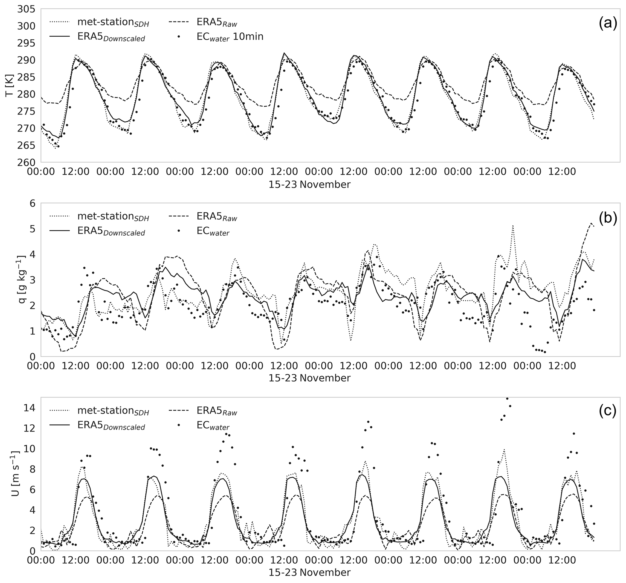
Figure 2(a) Data comparison of air temperature (T), (b) specific humidity (q) and (c) wind speed (U) between the available data sources: observations gathered from an eddy covariance (EC) over water surface (ECwater); observations collected from a meteorological station overland (met-stationSDH); ERA5 reanalysis raw data (ERA5raw); and ERA-5 reanalysis downscaled data (ERA5down).
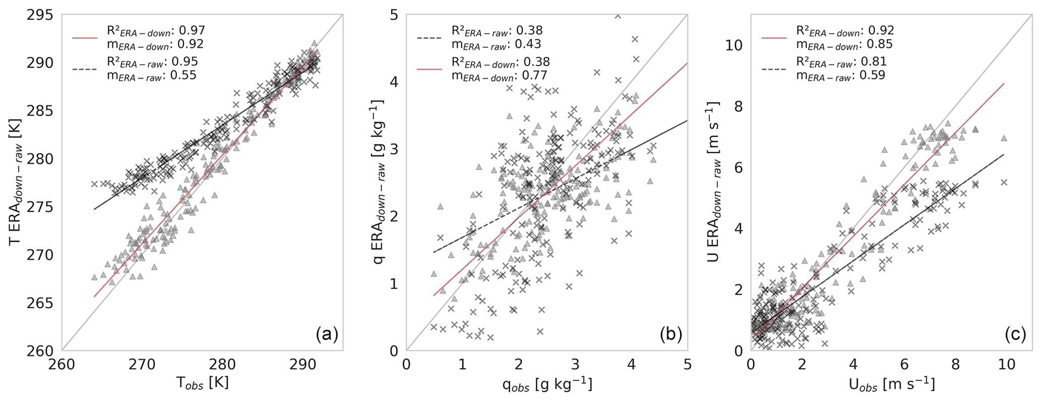
Figure 3Comparison between ERA-5 data before and after the downscaling against the met-stationSDH observations for (a) air temperature (T), (b) specific humidity (q), (c) and wind speed (U). Crosses represent the ERA5down data and triangles the ERA5raw data.
For q, there is more scatter in the met-stationSDH observations, which results in low R2=0.38 (Fig. 3b). However, similar to temperature, we observe an improvement after the downscaling, where ERA5 data increases the slope in the orthogonal regression from 0.43 to 0.77. Although the agreement between q-ERA5 and observations is lower than T-ERA5, q-ERA5 has a reasonable agreement with observations in the diurnal cycle (Fig. 2b).
In terms of U, we observe more differences between ECwater and met-stationSDH during the maximum values. The differences are related to the surfaces above which the instruments are installed, i.e., ECwater above the saline lake and met-stationSDH above bare soil (Fig. 1). However, our statistical calculations corroborate the benefits of using the downscaling methods: R2 increases from 0.81 to 0.92 and slopes from 0.59 to 0.85 as compared to ERAraw. Finally, although WD is not used to estimate the evaporation and not shown in the plots, the ERA5 data have good agreement with observations.
2.3.2 Actual evaporation estimation
To estimate the actual evaporation, we employ an adapted version of the Penman (1948) equation for open water evaporation (Huerta-Viso, 2021), expressed in energy terms LvE. Our approach is to use standard meteorological data of T, q, U and Swin from the downscaled ERA5 dataset, and apply it to the specific conditions of the SDH shallow lake. The adapted version of the Penman equation reads as
where s [Pa K−1] is the slope of the saturated vapor pressure curve, γ [Pa K−1] is the psychrometric constant, Rn [W m−2] is the net radiation, G [W m−2] is the ground heat flux, ρ [kg m−3] is the dry-air density, cp [] is the air's specific heat at constant pressure, ra [s m−1] is the aerodynamic resistance, esat [Pa] is the saturated vapor pressure, and ea [Pa] is the vapor pressure at measured level. The ice coefficient cice [–] is a correction coefficient that represents the evaporation reduction that occurs when an ice cover is formed above the saline lake (Vergara-Alvarado, 2017), and cEBNC [–] is the energy balance non-closure coefficient, which corrects the available energy (Rn−G) to improve the energy balance closure. Note that Eq. (1) becomes the Penman (1948) equation when . Appendix A describes the details of the calculation for each term in the Eq. (1).
2.3.3 Climatological analysis
To evaluate the diurnal variability of evaporation, the evaporation estimates are compared with observations using orthogonal regression, where we estimate the error employing the root mean squared error (RMSE), the mean absolute error (MAE), and the correlation (R) and determination (R2) coefficients. The climatology of evaporation estimates and precipitation data obtained from ERA5 are analyzed at seasonal and interannual scales. For seasonal timescales, we use descriptive statistics of mean, maximum, minimums and quantiles (25, 50 and 75) for each averaged month over the entire period (1950–2020). For the interannual timescales, we calculate monthly anomalies as the difference between the 12-month moving average and the mean of the entire period under study. Our reason for using the moving average is to decrease the high scatter that monthly means produce and better evaluate the ENSO and PDO influence on the evaporation and precipitation.
2.3.4 Large-scale moisture transport tracking model
To get an overview of the moisture transport that results in precipitation over the Altiplano region and surrounding areas, we selected the moisture sources of a selected region spanning from 83∘ W to 57∘ E, and from 11∘ N to 27∘ S (Fig. 7). For that, we use ERA-Interim data (Dee et al., 2011) from 1997–2018 to force the Water Accounting Model-2layers (WAM-2layers; van der Ent et al., 2010; van der Ent, 2014). The WAM-2layers is an Eulerian offline moisture tracking model which solves the atmospheric water balance for every grid cell. Tracking is performed on two layers in the atmosphere, hence the atmospheric input variables from ERA-Interim are integrated over two layers. Well-mixed conditions are assumed for both layers. More information on the model is given by van der Ent et al. (2010) and van der Ent (2014). Seasonal averages of moisture sources are evaluated (1997–2018; summer (JFM), autumn (AMJ), winter (JAS) and spring (OND)) together with the direction and intensity of the moisture fluxes.
2.3.5 Estimation of the long-term water balance of the lake
The long-term water balance in the saline lake is assessed by combining the mass conservation principle with actual evaporation estimates and precipitation data. Evaporation estimates are obtained using data from the downscaled ERA5 and the site-adapted Penman equation (Sect. 2.3.2), whereas precipitation data were obtained from the raw ERA5. The mass balance is evaluated as follows: first, the volume of the lake in a specific month is estimated using the lake's area (de la Fuente et al., 2021) and assuming a constant lake depth that varied between 0.05 and 0.20 m. Second, we estimate the monthly lake outflow using the actual evaporation values and the lake's area, assuming no groundwater outflow (endorheic basin). Third, we determine the volume reduction of the lake due to evaporation by subtracting the volume of water evaporated in a month from the volume of the lake. Then, the lake area of the next month is computed dividing the lake's volume by its depth. This area is compared to that obtained using remote-sensing data to determine the additional monthly water volume required to achieve the observed lake surface. By associating this additional water input with precipitation, we determine the areal extension of precipitation that contributes to the representation of the observed areas of the lake. Because most of the time there are no surface water inputs (negligible surface runoff is observed), this additional water source must represent groundwater inputs into the lake. The approach followed here is a first order approximation that can be used to understand the key components of the lake's water balance. However, we believe that more precise information is needed to reproduce the seasonal variability of groundwater flow.
This section describes the diurnal, seasonal and interannual variability of evaporation at the saline lake of SDH. First, we analyze the diurnal variability of evaporation through the site-adapted Penman equation. We then analyze the seasonal variations of evaporation, its main drivers and the role of evaporation in the water balance of the saline lake. Finally, we close the article by studying the climatological trends of evaporation–precipitation and the influence of the ENSO and PDO phenomena on their anomalies.
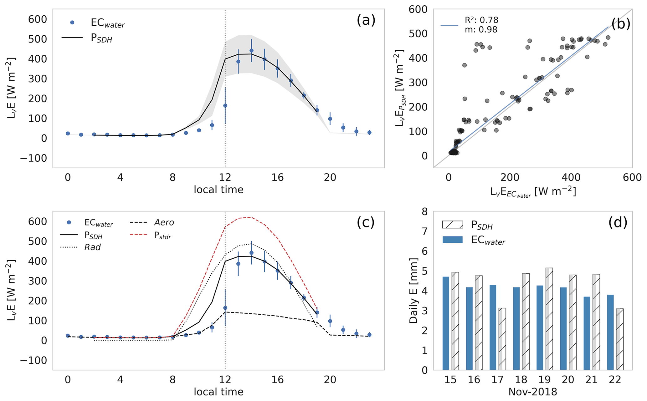
Figure 4(a) Daily average and standard deviation of LvE observed by ECwater and calculated by the PSDH equation during the E-DATA period. (b) Orthogonal regression between LvE measured by the ECwater and those estimated through PSDH. (c) Diurnal cycle of LvE observed by ECwater, calculated by PSDH, standard Penman (Pstdr), and the aerodynamic (Aero) and radiative (Rad) contribution. (d) Daily evaporation (mm) measured by the EC system and estimated through PSDH. The vertical dotted line in (a) and (c) indicates the wind regime change.
3.1 Diurnal cycle perspectives of evaporation
Figure 4 shows the averaged LvE diurnal cycle over the E-DATA period observed by the ECwater, calculated using the site-adapted Penman equation (PSDH, Eq. 1) and the standard Penman (1948) equation (Pstdr). Figure 4a and b indicate that there is a satisfactory agreement between observed and estimated LvE. The main difference is the 2 h lag during the morning transition (between 11:00 and 13:00 LT) that results from the height at which ERA5 wind is calculated: 10 m. These data have RMSE of 73 W m−2 and MAE of 17 W m−2. Likewise, the orthogonal regression of LvE between the PSDH and ECwater observations have acceptable R and R2 coefficients (R=0.88 and R2=0.78, respectively) and orthogonal regression slopes (m=0.98).
To better understand the LvE results obtained by PSDH, we analyze the radiative energy and aerodynamic contributions to Pstdr for LvE separately, along with the performance of the introduced coefficients. Figure 4c shows the averaged diurnal cycle of the energy and aerodynamic term of Pstdr, compared to the results of PSDH (Eq. 1) and the EC observations of LvE. The diurnal pattern of LvE shows two distinct regimes: in the morning (before 12:00 LT), the aerodynamic term follows the observations closely whereas in the afternoon (after 12:00 LT), the energy term is the one with a closer match. Our explanation is based on the limiting regimes which have been studied by Lobos-Roco et al. (2021), Lobos-Roco et al. (2022) and Suárez et al. (2020). During the morning, LvE is limited by the absence of mechanical turbulence. As a result, the transport from the saturated air above the surface into the dry atmosphere is hampered, which results in relatively low values for LvE. In turn, during the afternoon, due to the regional wind flow arrival, the enhancement of mechanical turbulence leads to high values of evaporation, and LvE depends on the amount of the available energy. This radiative energy control is more clearly observed from 14:00–15:00 LT when radiation decreases the LvE yields. The addition of energy and aerodynamic contribution to Pstdr shown in Fig. 4c (dashed red line) demonstrates an overestimation of 88 W m−2 concerning the observations, where the diurnal cycle is only followed during the afternoon (windy regime). When comparing the PSDH (Eq. 1) and Pstdr for LvE, we observe that coefficients significantly improve the evaporation estimates. This improvement is given first by the coefficient that reduces the available radiative energy under calm wind conditions, decreasing it by 70 % and 30 % under windy conditions. Secondly, the coefficient improves LvE estimations by mitigating the fluxes when the water in the lake is frozen to a factor of 0.3 (Appendix A4). Table 2 summarizes comparative statistical metrics between the results obtained using a Pstdr and PSDH equations with observations.
Table 2Statistical metrics for comparing standard Penman, site-adapted Penman, radiation and aerodynamic contribution for LvE, compared to LvE ECwater observations. Monthly evaporation integration compares site-adapted evaporation estimates performed using ERA5 and met-stationSDH during the period 2016–2020. ∗ Evaporation monthly integration comparison metrics are between PSDH estimates using ERA5 and observation from met-stationSDH (Table 1). The m represents the slope of the orthogonal regression between ECwater and estimated through the Penman equation.
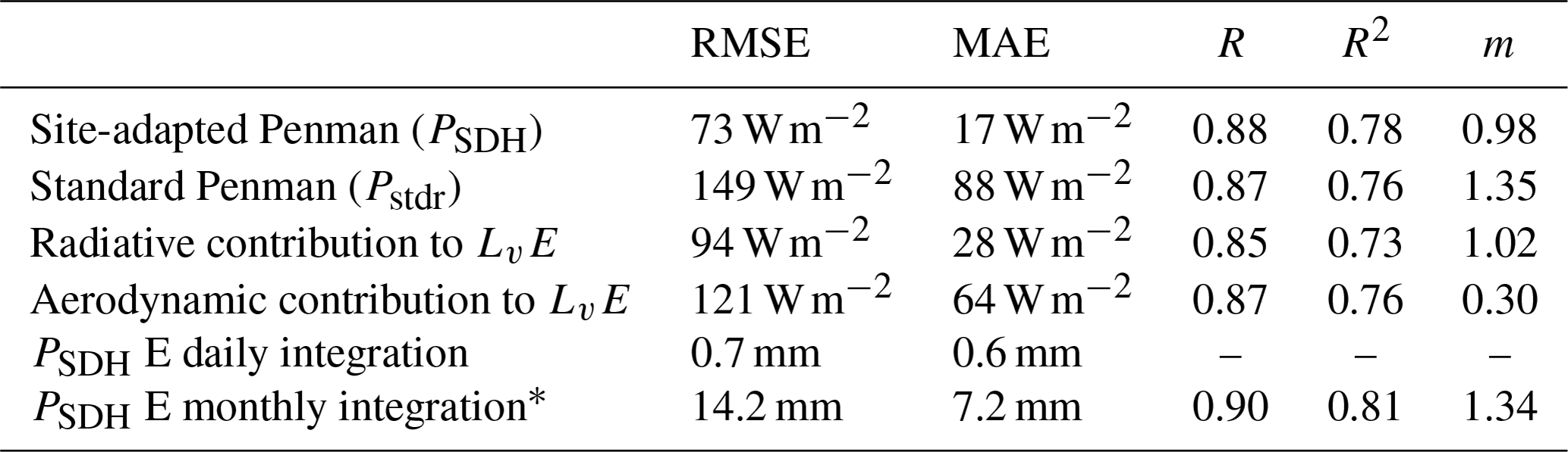
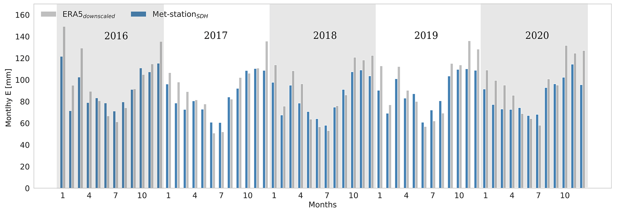
Figure 5Monthly integrated evaporation obtained through the site-adapted Penman equation using ERA5 and met-stationSDH standard meteorological data during the 2016–2020 period.
Finally, in Fig. 4d, we integrate sub-diurnal evaporation estimates for validating our results during the entire E-DATA period. The Figure shows the daily evaporation between the EC observations and PSDH. Daily values show differences of ∼0.65 mm between observations and estimations (RMSE: 0.7 mm; MAE: 0.6 mm). Integrating the whole E-DATA period, the differences are ∼5 mm: 38 mm for PSDH and 33 mm for ECwater. To place these differences into perspective, it is worth noting that our focus in this research is to study the climatology of the evaporation in this region. As such, we consider that mean daily errors below 1 mm d−1 are low enough to use Eq. (1) using the ERA5 downscaled data for long-term actual evaporation estimations.
Nevertheless, to extend our validation into a longer period analyzed in Sects. 3.2 and 3.3, Fig. 5 shows the LvE calculated using two methods: (1) the site-adapted Penman monthly evaporation estimates using ERA5 downscaled data and (2) observations from the met-stationSDH between 2016–2020. We find a good agreement between both estimates. The results show that ERA5 follows the seasonal cycle (R2: 0.81) satisfactorily. However, ERA5 evaporation overestimates the observations by 7.6 %, which is consistent with the overestimation that ERA5 reported for evaporation results with respect to the EC observations during the E-DATA period (6.1 %).
The previous evaluation provides enough support to use the site-adapted Penman evaporation results to count with high-quality long-term (1950–2020) actual evaporation estimates at local (saline lake) scales and high time resolution (1 h).
3.2 Seasonal perspectives of evaporation and precipitation
Evaporation estimated sub-diurnally through the Penman equation also presents significant seasonal changes that can have high impacts on water resources. This section first analyzes the seasonal cycles of actual evaporation by describing the changes in its radiative and aerodynamic contributions. In addition, we include the precipitation in the analysis as an essential component in the water balance. Secondly, we analyze the seasonal evaporation and precipitation impacts on the water balance of the saline lake of SDH.
3.2.1 Evaporation and precipitation seasonal cycles
Figure 6a shows the actual evaporation seasonal average from 1950 to 2020 over the saline lake of SDH. In general, seasonal changes of evaporation show their highest monthly values (>90 mm) during the austral summer (JFM) and spring (OND). Within these seasons, October, November and December present the highest monthly evaporation (107–120 mm). Even though the summer also presents high monthly evaporation (90–107 mm), these months also show the highest variability (standard deviation of 13.5–16.5 mm). The variability observed during the summer months is because of the rainy season that usually extends over the summer (Vuille et al., 2000; Garreaud et al., 2003). Evaporation has its lowest rates during autumn and winter (<78 mm per month). Moreover, within these seasons, the months of June, July and August show the lowest monthly evaporation (∼50 mm) and the lowest variability of the year (standard deviation of 7 mm per month). On the other hand, the seasonal variability of precipitation is shown in Fig. 6b. Precipitation in the SDH basin shows a very clear seasonal cycle, with the onset of the rainy season in late spring (ND) and the offset at the end of summer (MA). However, this rainy season presents high variability over the years. The rest of the seasons show precipitation values below 25 mm per month, where June and July present a slightly higher variability.
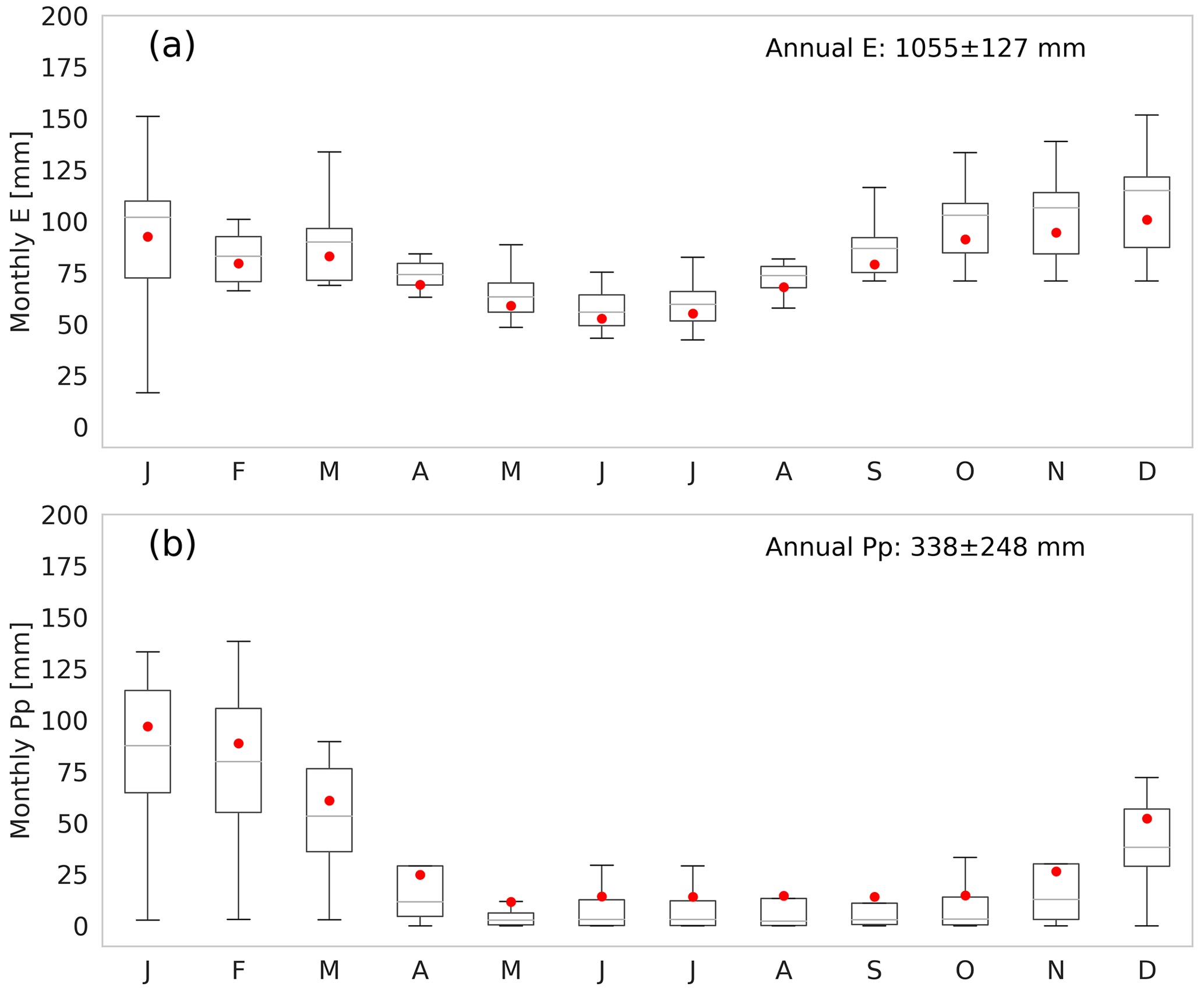
Figure 6Seasonal variability of monthly (a) evaporation (E) and (b) precipitation (Pp) rates during the 1950–2020 period. The boxes represent the 25 %–75 % interquartile, the gray horizontal line is the median, the red dots are the mean, and the bars represent maximum and minimum values. Outliers have been removed and annual evaporation and precipitation have been calculated over the entire period.
To give a synoptic-scale perspective of the seasonal changes in local evaporation and precipitation presented in the saline lake of SDH, Fig. 7 shows the seasonally averaged moisture sources of the Altiplano region. Here, we quantify the regions where evaporation occurs which results in precipitation over the Altiplano region (gray box in Fig. 7). As most precipitation occurs in the austral summer (Fig. 6), the moisture sources are also largest in these seasons. We observe three principal moisture sources that contribute to precipitation in the Altiplano region during the year. The first one comes from the northeast (Amazon basin) and results from the veering of trade winds southwestwardly into the Andes Mountains, associated with the continental low formed by the summery position of the Intertropical Convergence Zone (ITCZ) south of the Equator (Aceituno, 1992). This southwestward flux is most pronounced during summer, transporting moisture (∼50 mm) into Altiplano region. This marked moisture flux suddenly decreases towards the autumn and winter (∼10 mm). During these seasons, the trade winds return to their normal westwardly direction (Fig. 7b and c), resulting in low moisture transport (∼20 mm) into the region. Besides moisture transport into the region from the northeast, there is also recycling of moisture within the region, which can be considered to be a second moisture flux. Especially during summer, evaporation contributes to precipitation within the region, as can be seen by the high moisture source values around the lake in SDH during JFM and OND (Fig. 7a and d). In addition to the contributions from evaporation over land, there is also a positive moisture source from the Pacific Ocean (south–southwest). In the absence of precipitation over the ocean, we can assume that the evaporation over the ocean contributes to the precipitation over land in the Altiplano region. Finally, this third moisture flux is associated with the subtropical anticyclone and stratocumulus cloud deck (Rutllant et al., 2003; Lobos-Roco et al., 2018). This flux transports a very low but persistent amount of moisture into the Altiplano region (<5 mm) due to the steep topography presented on the western slope of the Andes Mountains, which in combination with the anticyclone, limits the eastward flow up to the mountains. Despite the coarse model resolution, this low-moisture transport has been reported using high-resolution modeling and airborne observations by Suárez et al. (2020) and Lobos-Roco et al. (2021).
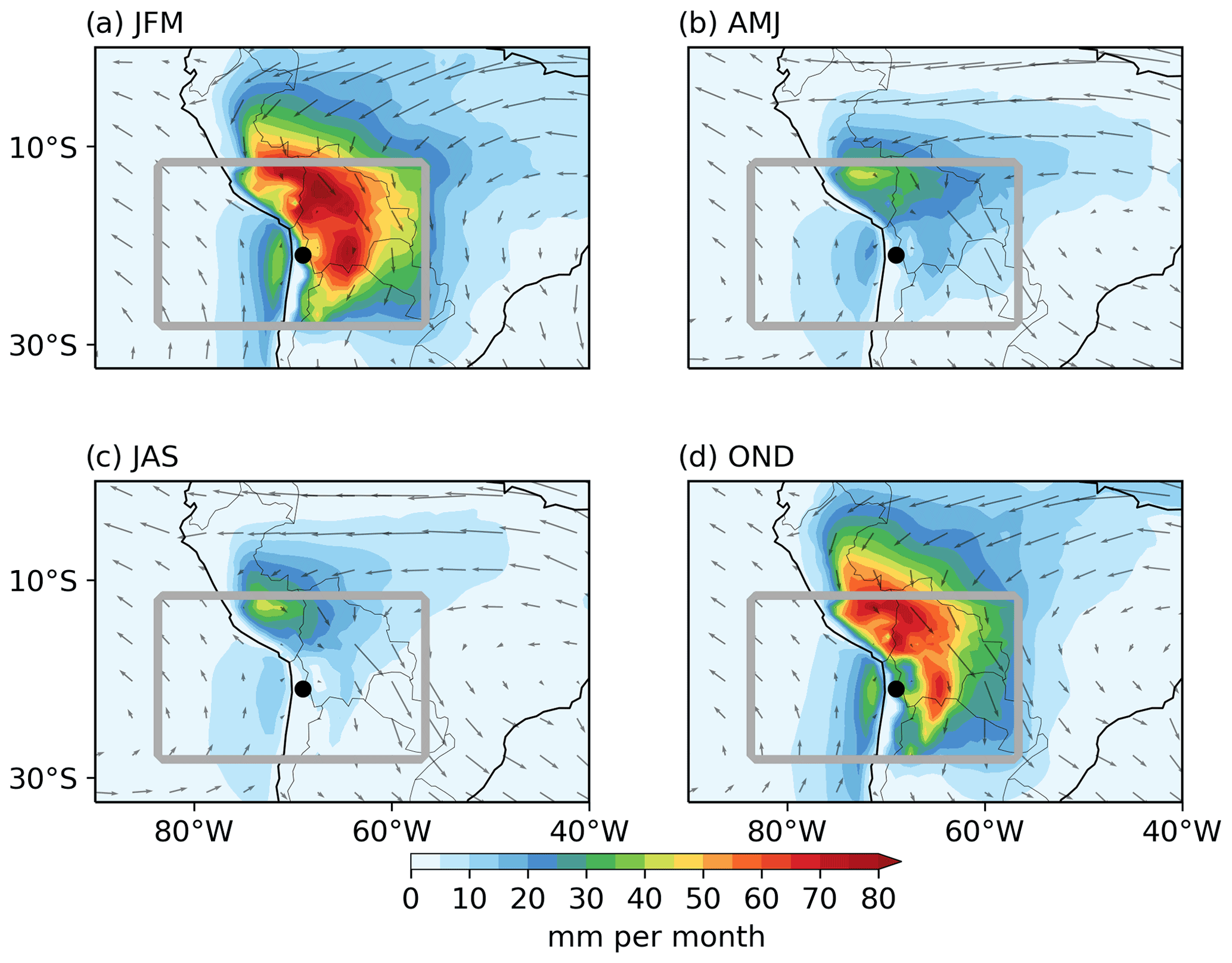
Figure 7Seasonal variability of moisture sources (shaded) in mm per month and vertical integrated moisture transport (arrows) over the Altiplano region for (a) summer, (b) autumn, (c) winter and (d) spring. The gray squares frame the Altiplano regions and surroundings for which the sources are determined. The black dots indicate the Salar del Huasco location.

Figure 8(a, c) Seasonal variability of radiative and aerodynamic contribution to evaporation during the period 1950–2020. The boxes represent 25 %–75 % interquartile, the gray horizontal line is the median, the red dots are the mean and bars represent maximum and minimum values. Outliers have been removed. (b, d) Orthogonal regression of evaporation rates and its energy and aerodynamic contribution at averaged monthly scale.
To unravel the processes involved in the seasonal evaporation, we analyze the seasonal variability of the drivers that control it. Figure 8 shows the seasonal cycle of the radiative and aerodynamic contribution of the Penman equation and subsequent correlations with monthly evaporation rates.
Figure 8a shows the seasonality of the radiative contribution to evaporation, with its highest values corresponding to spring and summer, slowly decreasing towards the winter, only to increase again in early spring. The seasonality of the radiative contribution is similar to that of evaporation shown in Fig. 6b, but it presents two distinctive characteristics. Firstly, from November to March, there is a larger scatter (standard deviation >12 W m−2), where the radiative contribution to evaporation can be high at 170 W m−2 or low at 20 W m−2. This large variability is directly related to the summer rainy season (Vuille et al., 2000), where the presence of clouds largely modulates the available net radiation (Houston, 2006). This double feedback that precipitation has over the radiation might explain the large scatter in the radiative contribution to evaporation during spring–summer. Secondly, the small variability (standard deviation of ∼3 W m−2) of the radiative contribution during the winter months is related to the atmosphere's stability, characterized by the dry weather and cloudless conditions during most of this period. Therefore, there is enough evidence to support the idea that radiative contribution controls evaporation at a seasonal scale (R2=0.91, as shown in Fig. 8b).
Figure 8c shows the seasonality of the aerodynamic contribution to evaporation, where the highest and lowest values are observed in early spring (SON) and during summer (JFM), respectively. The variability of the aerodynamic contribution is fairly constant during the whole year (standard deviation of ∼4 W m−2), which is related to the seasonality of the wind circulation patterns (Falvey and Garreaud, 2005). The wind seasonality also explains the highest and lowest aerodynamic contribution to seasonal evaporation. For example, the thermal contrast between the Pacific Ocean and the Atacama Desert reaches its maximum in November, resulting in the strong regional atmospheric eastward flow, responsible for the onset of diurnal evaporation in the SDH (Lobos-Roco et al., 2021). To the contrary, during summer, predominant westward regional circulation from the Amazon basin counteracts the eastward regional flow (Garreaud et al., 2003), decreasing the wind speed (as described below). Finally, during winter, the lower thermal contrast between the Pacific Ocean and the Andes Altiplano, along with the absence of the summer westward regional flow, results in lower wind speed. Consequently, there is less aerodynamic contribution to evaporation. The scattered seasonality of the aerodynamic contribution to evaporation also results in a low correlation (R2=0.34, as shown in Fig. 8d).
In summary, at the seasonal timescale, the radiative contribution term contributes significantly more to evaporation than the aerodynamic term, representing 73 % of the energy needed to evaporate the water from the saline lake in SDH. It is important to stress that mechanical turbulence (wind speed) is more relevant at the diurnal scales than available net radiation controlling evaporation (Lobos-Roco et al., 2021).
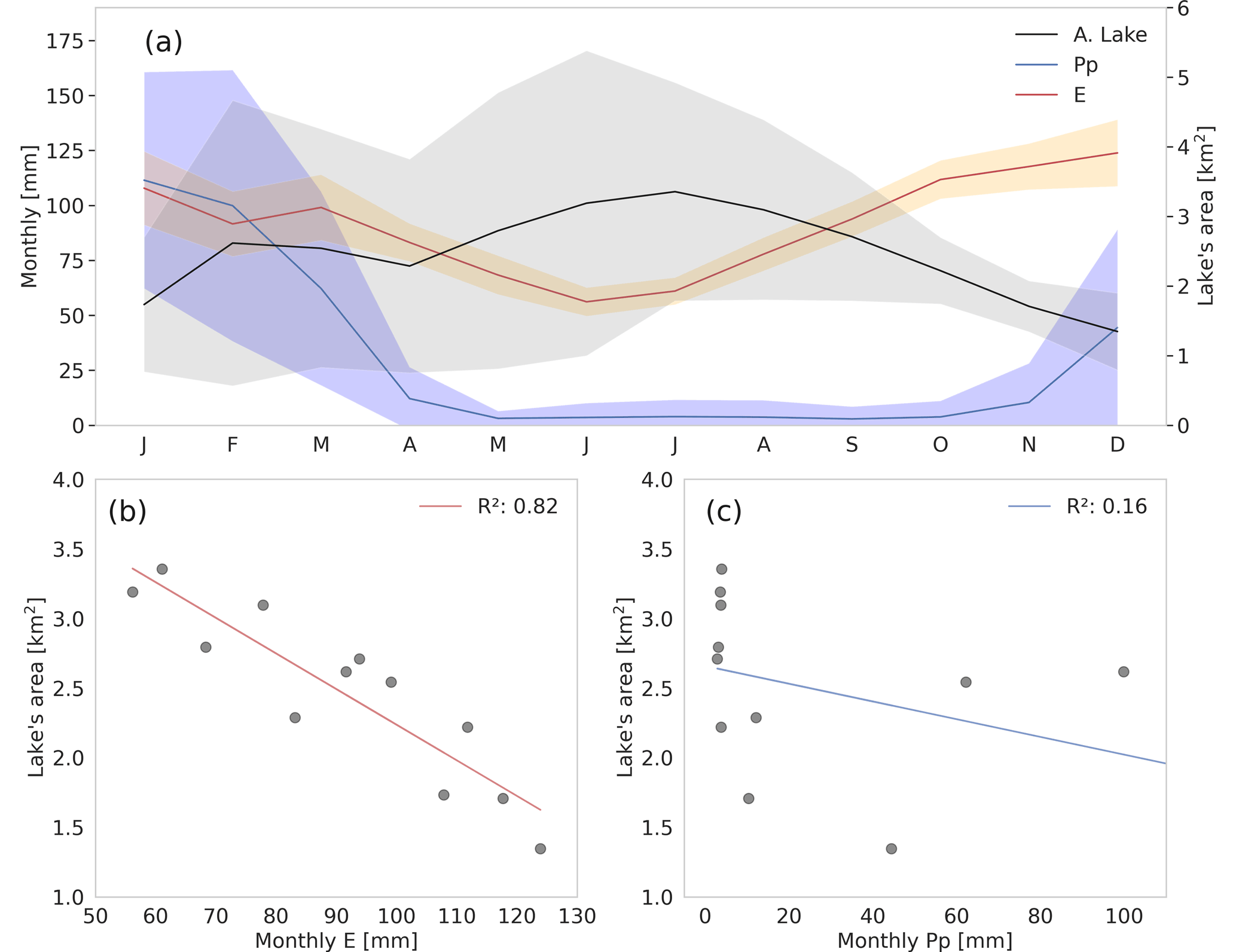
Figure 9(a) Monthly mean variability of lake's area, total evaporation (E) and total precipitation (Pp). Shades indicate the standard deviation of each variable. (b) Monthly orthogonal regression between lake's area and monthly evaporation. (c) Monthly orthogonal regression between lake's area and monthly precipitation.
3.2.2 Seasonal changes in the saline lake's water balance
To complete the seasonal analysis of evaporation in recent decades, we describe the spatial impacts of the evaporation–precipitation variability on the saline lake of SDH. Before showing the results, it is interesting to mention the heterogeneous characteristics of open waters and different types of salty crusts (Kampf et al., 2005). These salty crusts cover larger areas than open-water surfaces, contributing significantly to the basin's water balance. With respect to the wet/dry salt contribution, the salt crust found in SDH has particularly low evaporation (<50 W m−2, e.g., see Lobos-Roco et al., 2021, Fig. 3b). Despite this low rate, it is still relevant since the open-water/wet salt surface proportion has high seasonal variability. Based on our flux data (4.3 mm d−1 for open water and 0.5 mm d−1 for wet salt) and surface areas estimated from satellite remote-sensing observations in November (1.8 km2 for open water and 13.1 km2 for wet salt), we estimate that open-water evaporation is 7.8 against 5.6 m3 d−1 for wet salt. In the rest of the section, we focus on the saline lake's water balance as an entity integrating the different contributions. Figure 9 shows the relationship between the spatial changes of the saline lake and monthly evaporation and precipitation that occurred between 1985 and 2019. The seasonal variability of the lake's area shown in Fig. 9a reveals that the maximum extension (5 km2) occurs during winter (JJA). During spring, the lake's area decreases rapidly to its minimum extension (∼1.3 km2). The summer season shows high variability in the lake's area (mean: 2 ± 1.8 km2; mean value ± standard deviation). This variability is relatively constant towards winter and decreases during spring, revealing that there is a significant interannual variation over the years, especially between March and July, where precipitation is typically small (Fig. 6d). Thus, the increase in the lake's area is likely due to groundwater inputs (Blin et al., 2022).
Regarding the relationship between the lake's area changes and evaporation, Fig. 9b shows an orthogonal regression between evaporation and lake extension changes. Here, we find a strong negative correlation (R2=0.92), which reveals the control that evaporation has over the lake discharge. The lowest evaporation rates (winter) coincide with the highest lake extensions, and the highest evaporation rates (spring) coincide with the lowest lake surface. Regarding the relationship between precipitation and the lake's surface associated with the water recharge by precipitation, the relationship is indistinctive (Fig. 9a). We find a high variability in the onset and offset of precipitation at the seasonal scale, from November to March. This high variability in summer precipitation coincides with the larger variations in the lake's area. As such, it is difficult to find a direct relationship between precipitation and the lake's area. However, analyzing the means (solid lines Fig. 9a), we observe that high precipitation rates do not directly impact the areal changes of the lake. In February, the lake's surface reaches a first maximum, which might be related to precipitation in the direct proximity of the lake, generating enough surface runoff to enhance the water amount of the lake. However, the highest values of the water-lake surface is reached 4–5 months after the rainy season. For these reasons, the observations suggest that there is another process that modulates the lake recharge. Thus, the alternative that explains lake recharge is groundwater, which is fed by precipitation in the headwaters of the basin.
To unravel the role of groundwater input into the SDH lake, we perform a simple lake water balance test assuming a lake depth between 0.05 and 0.20 m. Our lake mass balance results show that the monthly water required to represent the spatial changes in the lake's surface are in the order of ∼345 000 m3 per month (∼0.1 m3 s−1). This estimation is reasonable as the only stream flowing in the lake direction has an average flow of 0.13 m3 s−1 (Blin et al., 2022), which is measured about 1–2 km before the river water completely infiltrates into the ground. If one assumes that ERA5 precipitation is responsible for this water flow, then a lake area of ∼13 km2 is needed to explain it. When varying the water depth between 0.05 and 0.20 m, our results changed less than 1 %. As the mean observed lake's area is ∼2 km2, groundwater is the water source that sustains this habitat. This result agrees with the estimations performed by Blin et al. (2022). They quantified a flow in the range of 0.14 to 0.2 m3 s−1 in the springs that discharge water into the lake, which is similar to the flow estimated in our work. It is important to recall that our approach has important limitations. For instance, as the topography in the basin's sink is very flat, there is no hypsometric curve that can relate the lake's volume as a function of depth. Also, the precipitation considered here corresponds to that estimated in the lower part of the basin, whereas higher precipitation values occur at higher elevations in the basin (Uribe et al., 2015; Blin et al., 2022). Hence, most of the groundwater recharge is expected to occur at higher elevations and/or in locations where preferential flow exists, e.g., near the rivers of the basin. Then, this water will flow underground until it upwells into the lake. So, even though this approach has limitations, it allows for a first order approximation that can be used to understand the key components of the lake's water balance.
3.3 Interannual perspectives of evaporation and precipitation
3.3.1 Climatological trends of evaporation–precipitation
Evaporation trends in the saline lake of SDH show an indubitable increase from 1950 to 2020. The rate of increase is about 2.1 mm yr−1 (0.2 mm per month), with scattered interannual variability showing a significant increase. Figure 10a shows a 12-month moving average of monthly total evaporation. For 1950, monthly mean values are approximately 80 mm (950 mm yr−1), whereas in 2020, these values increased to ∼100 mm (1150 mm yr−1). The annual integrated evaporation rates averaged 1075 mm (±74 mm) with a minimum of 862 mm (1993) and a maximum of 1210 mm (2010). This increase in evaporation has a correlation of 0.55 with air temperature (2 m), whose monthly averages increased 3 ∘C (0.04 ), from 1950 to 2020 (Fig. 10a). Likewise, Fig. 10b shows the precipitation trends in the area of the saline lake from 1950 to 2020. Total precipitation per year is set at 338 mm with a high variability of 248 mm yr−1. Precipitation shows an increasing trend of 0.6 mm yr−1 in the last 70 years. Although this positive trend in precipitation is less significant than evaporation and presents more scatter, it is also in agreement with temperature increase.

Figure 1012-month moving average monthly total (a) evaporation (E) and (b) precipitation (Pp) and 2 m mean air temperature (T) over the saline lake of SDH from 1950 to 2020. The long-term trend is indicated by the red line.
3.3.2 Influence of ENSO and PDO phenomena on evaporation–precipitation
Figure 11 shows the seasonal variability of monthly evaporation in the period 1950–2020 during cool ( ∘C), neutral ( ∘C) and warm (ONI>0.5 ∘C) ENSO phases. In general, during cool ENSO phases, evaporation rates are 2 % lower than those observed in the neutral ENSO phases, whereas during warm ENSO phases, evaporation is 15 % higher than that observed in neutral ENSO phases. This variability becomes more significant from October to May, summer (JFM) being the season with the largest variability. During summer, evaporation under cool ENSO phases decreases by 4 % with respect to neutral phases and increases by 14 % under warm conditions. Moreover, summer variability is the highest during warm ENSO phases, showing standard deviations of ∼15 mm per month. The lowest evaporation variability occurs during the neutral phases, with standard deviations of 11 mm per month. In turn, during late autumn and winter seasons, the ENSO phenomenon influences the evaporation less in the saline lake of SDH since evaporation rate differences between cool, neutral and warm phases are lower than 2 %. This analysis suggests that ENSO significantly influences evaporation during summer months, which is in line with other typical meteorological phenomena of the Atacama Desert, such as summer precipitation (Aceituno, 1988) and coastal fog formation (del Río et al., 2021).
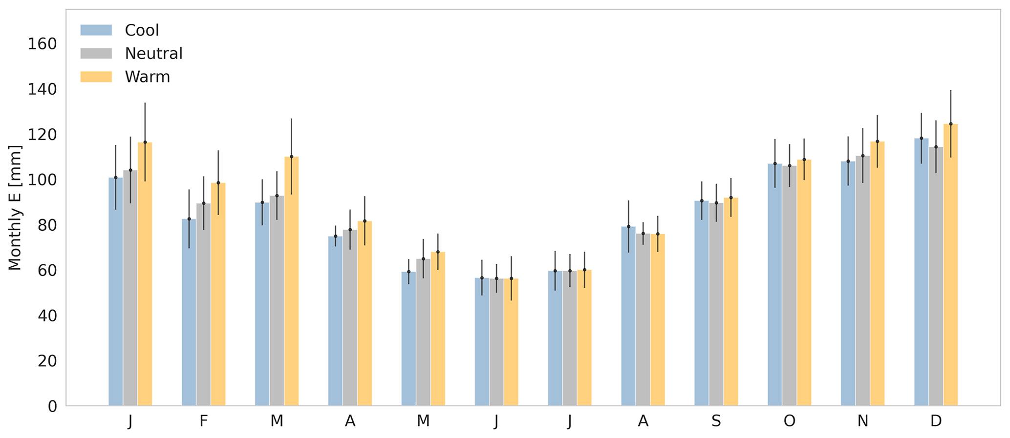
Figure 11Interannual–seasonal variability of monthly evaporation in the period 1950–2020 separated by cool, neutral and warm ENSO phases. Error bars represent the standard deviation of every averaged month.
The ENSO phases' influence on evaporation observed at the seasonal scale is also present interannually. Figure 12 shows the relationship between ENSO phases and PDO phenomenon, with evaporation anomalies obtained using the site-adapted Penman equation (Eq. 1) and downscaled ERA 5 data, and precipitation anomalies observed from ERA5 in the last 7 decades in the shallow lake of SDH. Recall that ENSO is a recurrent phenomenon with an ill-defined periodicity, where in the last 70 years, 24 % of the months have been influenced by warm ENSO phases and 26 % by cool ones. However, the frequency of this phenomenon is not constant, neither in intensity nor in time. The ONI varied between 0.5 and 2.6 ∘C during warm phases, and between −2 and −0.5 ∘C during cool phases, with a frequency between 2 and 10 years (Timmermann et al., 2018).
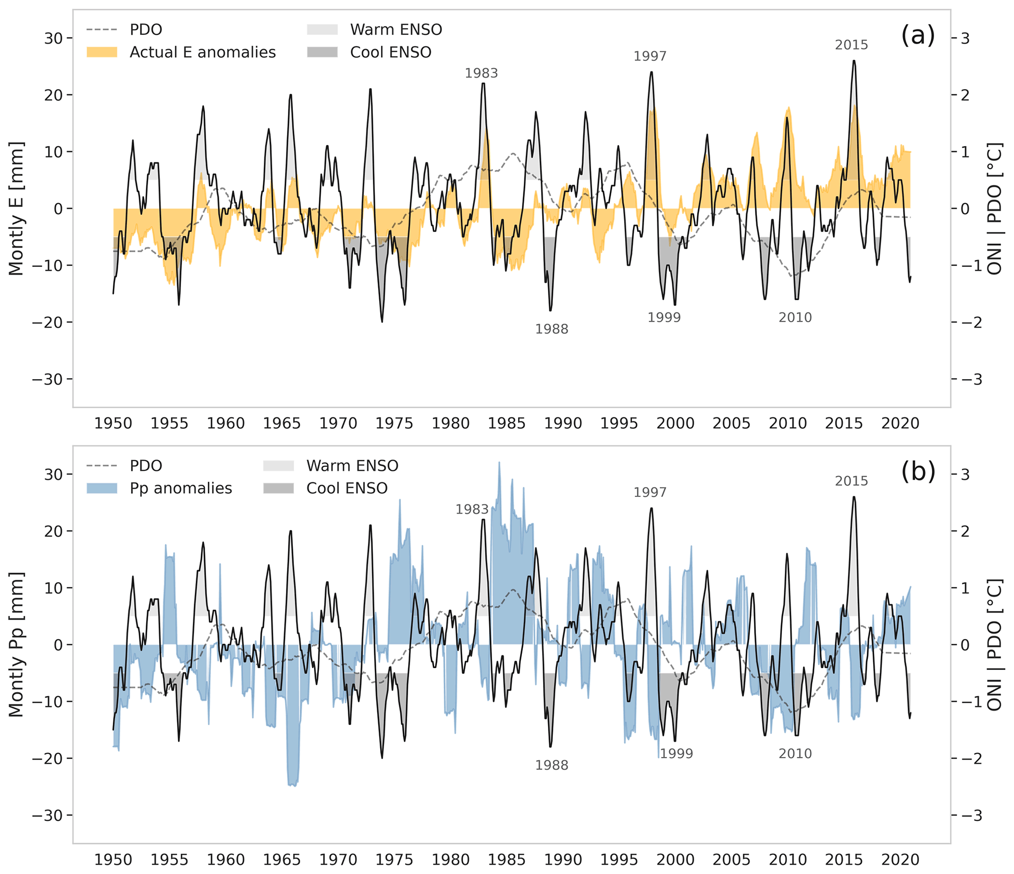
Figure 12(a) Monthly evaporation (E) anomalies compared to ONI and PDO indices. (b) Monthly precipitation (Pp) anomalies compared to ONI and PDO indices. Anomalies are calculated using the difference between the entire period mean, and 12-month moving averaged anomalies. Evaporation and precipitation anomalies are shown in colors: the ONI with a solid black line, highlighting the warm and cool phases, and PDO with a dashed line.
Figure 12a shows the 12-month moving average evaporation anomalies and the ENSO and PDO phenomena from 1950 to 2020. Positive monthly evaporation anomalies (>5 mm) correlate with warm ENSO phases, whereas negative or non-evaporation anomalies (<0 mm) correlate with cool ENSO phases. The correlation between positive evaporation anomalies and warm ENSO phases is evident during the extreme ENSO events, i.e., events which occurred in 1983, 1997 and 2015. Similarly, the correlation between negative evaporation anomalies and cool ENSO phases is evident in 1988, 1998 and 2010. However, this trend is indistinct when monthly evaporation anomalies are close to 0 mm (e.g., in 1970, 1995 and 2001). Evaporation anomalies also have an interdecadal variability. For instance, between 1950 and 1975, negative evaporation anomalies dominate. On the contrary, between 2000 and 2020, positive evaporation anomalies dominate, but only after a transition period that occurred between 1975 and 2000, where both positive and negative evaporation anomalies are present. Regarding larger macroclimatic phenomena, no significant correlation is found between PDO and evaporation anomalies.
The influence of the ENSO phenomenon also affects precipitation at SDH. Figure 12b shows the 12-month moving average precipitation anomalies and the ENSO and PDO phenomena from 1950 to 2020. The influence of ENSO on precipitation is the opposite of that observed for evaporation. Here, positive monthly precipitation anomalies (>5 mm) correlate with cool ENSO phases, whereas negative monthly precipitation anomalies (<5 mm) correlate with warm ENSO phases. Contrary to evaporation anomalies, the relationship between precipitation and extreme ENSO events is indistinctive. For example, strong precipitation anomalies observed in 1985 disagree with an extremely cool ENSO phase. The same occurs for the extremely cool ENSO phase that occurred in 1999, where the precipitation anomaly is not correlated with high positive precipitation anomalies. However, the negative correlation trend between ENSO phases and precipitation anomalies is still evident. Precipitation anomalies also have an interdecadal variability that seems to be related to PDO anomalies. For example, between 1950 and 1970, there is a predominance of negative precipitation anomalies, which correlate with negative PDO indices. However, between 1970 and 2000, positive precipitation anomalies predominate along with positive PDO indices. Finally, between 2000 and 2020, negative precipitation anomalies predominate together with negative PDO indices. The negative relationship between precipitation and ENSO phases in the Altiplano region has also been reported by Aceituno (1988), Vuille et al. (2000), and Garreaud and Aceituno (2001).
To further quantify the opposing trend between evaporation and precipitation, Fig. 13 shows the relationship between evaporation and precipitation anomalies categorized by ENSO phases. The trend between cool ENSO phases and negative evaporation anomalies is significant ( mm), although it is weaker during extremely cool phases. Similarly, the trend between warm ENSO phases and positive evaporation anomalies is very clear, even during the most intense warm ENSO phases (>15 mm). Regarding precipitation anomalies, the trend shows a similar pattern, where negative precipitation anomalies ( mm) are related to extremely warm ENSO phases, and the highest positive precipitation anomalies are related to both cool and neutral ENSO phases.

Figure 13Relationship between monthly evaporation (E) and monthly precipitation (Pp) anomalies between 1950 and 2020. The anomalies are classified into warm, neutral and cool ENSO phases. The symbol size reflects the ONI intensity, where ONI≥1 corresponds to an intense warm phase (circle) and to an intense cool phase (triangle).
Opposing behavior of ENSO influences on interannual evaporation and precipitation variability demonstrate the control that global climate phenomena can exert at a local scale in the long term. As shown in Fig. 10a, air temperature is strongly related to evaporation; thus, atmospherically warmer conditions in the Altiplano region during warm ENSO phases enhance evaporation. This warming intensifies the Pacific anticyclone through the tropospheric thermal stratification (Falvey and Garreaud, 2009), resulting in cloudless conditions during the summer of warm ENSO phases, i.e., an increase in the radiative contribution term of 17 % as compared to the cool phases. Increased radiation also leads to an enhancement of the ocean–land thermal contrast, enhancing the aerodynamic contribution to evaporation by 21 % during warm ENSO phases in summer with respect to cool ENSO phases. This enhanced ocean–land thermal contrast also increases the atmospheric capacity to hold water vapor. Conversely, cool ENSO phases promote higher precipitation rates through the weakening of the Pacific anticyclone and the strengthening of the Bolivian low (Aceituno, 1988), which negatively affects the evaporation in two ways. First, the cloudy conditions that result from wet seasons inhibit the available energy required for evaporation (from 120 to 100 W m−2), mainly affecting the evaporation rates during the summer season (Fig. 11) as well as interannual rates (Fig. 10a) (Houston, 2006). Second, during cool ENSO phases, a strong rainy season attenuates the characteristic regional atmospheric flow from the Pacific Ocean into the Andes (Lobos-Roco et al., 2021), significantly affecting the aerodynamic contribution to evaporation (Fig. 8b), decreasing it from 38 to 30 W m−2.
We investigate the temporal changes of actual evaporation from sub-diurnal to climatological scales in a high-altitude saline lake ecosystem in the Atacama Desert. To this end, we combine observations of evaporation with two different model approaches. The first one downscaled ERA5 meteorological data (1950–2020) into local conditions observed at the saline lake of SDH using ANNs. The second one uses this downscaled data into a site-adapted Penman equation for open-water evaporation. The intercomparison between our estimates and direct EC evaporation measurements, taken in a dedicated 10 d field experiment, shows a good sub-diurnal agreement (R2: 0.78, m: 0.98) and errors of ∼7 % at diurnal and seasonal timescales.
Our first results reveal that ERA5/Penman successfully estimates open-water bodies' actual evaporation from sub-diurnal to interannual scales. In analyzing the budget of evaporation at the sub-diurnal scale, the wind speed (aerodynamic contribution) is the main driver of evaporation.
Our findings show significant seasonal variations. Maximum rates are reached during spring (OND), minimum ones during winter (JAS) and a high variability is observed during summer (JFM). The seasonal changes in evaporation are explained by 73 % to the radiative contribution of the Penman equation, where seasonal changes in incoming radiation play a dominant role in the available energy for evaporation. In addition, our local estimates of evaporation and precipitation over the saline lake correlate with synoptic and seasonal variabilities of moisture transport. In analyzing this transport, we identify three main large-scale fluxes that contribute to the available moisture in the Altiplano region. The principal one transports a significant amount of moisture from the northeast (Amazon basin) and the humidity recycled from the evaporation–precipitation process during spring and summer. The third moisture flux identified transports a very low but persistent amount of moisture from the Pacific Ocean into the Atacama Desert consistently over the year. This moisture flux is strongly limited by the subtropical anticyclone and the steep topography. In addition, the seasonal variation in evaporation and precipitation along the analyzed period impacts the saline lake. Our analysis suggests that evaporation is the principal driver of the lake discharge, explaining 92 % of it. However, the recharge of the lake still remains unknown, since the role of precipitation continues to be elusive and has not yet been quantified. By analyzing the saline lake's mass balance, we conclude that the water input required to explain the lake's spatial changes significantly exceeds that of precipitation. Therefore, we conclude that groundwater inputs play an essential role in the lake recharge.
Evaporation also present an interannual variability, where the ENSO phenomenon plays an important role. Our results reveal that ENSO phases affect the evaporation rates during the summer: warm phases increase evaporation by 15 %, whereas cool ones decrease it by 4 %. Concerning the driving components of evaporation, radiation controls these interannual changes in summer. This control is given by the cloudy or cloudless conditions that characterize ENSO cool and warm phases, respectively. However, this is also explained by the aerodynamic contribution during the cold phases. The weakening of the Pacific Ocean anticyclone promotes the entrance of wet eastern flow that decreases the usual westerly flow, affecting the contribution of wind to evaporation. Analyzing the evaporation and precipitation anomalies compared to ONI, we find that ENSO phases correlate positively to evaporation anomalies but negatively to precipitation ones. These correlations express that warm ENSO phases are characterized by higher evaporation rates and lower precipitation, whereas cool phases are characterized by lower evaporation and higher precipitation. In addition, climatological trends show that evaporation has increased by 2.1 mm yr−1 during the entire study period according to global temperature increases.
Finally, our study gives a first multi-scale temporal approach to understand actual evaporation, its role in the water balance of the saline lakes of the Atacama Desert, under a context of climate change. We demonstrate that long-term actual evaporation is estimated reliably through a simple approach that combines observations and reanalysis data. However, we acknowledge the need of longer-term actual evaporation measurements to reduce the 7 % uncertainty that the site-adapted Penman equation brings. Our approach aims at improving water resources management in arid regions. To generalize our approach, further research will be needed on the site-adapted Penman equation coefficients for other surfaces in the Atacama Desert (wet salt, wetlands and sparse vegetation lands), as well as other arid regions worldwide. Moreover, the interannual variability of evaporation–precipitation and moisture transport must be analyzed using higher-spatial-resolution models that include better local impacts related to the sharp topography and land-use changes, as well as the ENSO phenomenon. Lastly, our site-adapted Penman approach must be corroborated in basins and lakes with different spatial scales, topography and locations.
Here, we introduce the radiative and aerodynamic contributions to the Penman (1948) equation. We also provide a physical meaning to the two coefficients used in the modified Penman equation: the coefficient to compensate for the absence of surface energy balance closure (cEBNC) and the coefficient to account for the ice conditions (cice) above the saline lake of SDH. Note that some physical processes such as the effect of salinity on evaporation, are implicitly included in the site-adapted Penman equation. The empirical coefficients in the model are obtained using evaporation fluxes measured over the saline water surface (Suárez et al., 2020; Lobos-Roco et al., 2021). The modified Penman equation reads as
where s [Pa K−1] is the slope of the saturated vapor pressure curve, γ [Pa K−1] is the psychrometric constant, Rn [W m−2] is the net radiation, G [W m−2] is the ground heat flux, ρ [kg m−3] is the dry-air density, cp [] is the air's specific heat at constant pressure, ra [s m−1] is the aerodynamic resistance, es [Pa] is the saturated vapor pressure, Ta [K] is the air temperature and e [Pa] is the vapor pressure at a measured level. Below, we detail the calculation and justification of each term in Eq. (A1).
A1 Radiative contribution
The radiative contribution to the latent heat determined from Eq. (A1) depends on the available energy, i.e., Rn−G. Net radiation, Rn, is estimated as
where Swin [W m−2] is the incoming short-wave radiation, which is provided by the ERA5 dataset (Hersbach et al., 2020); Swout [W m−2] is the outgoing short-wave radiation; α=0.13 [–] is the albedo, obtained during the E-DATA field campaign (Suárez et al., 2020; Lobos-Roco et al., 2021); Lwin [W m−2] is the incoming long-wave radiation; and Lwout [W m−2] is the outgoing long-wave radiation.
The Lwin, which includes the cloud influence, is calculated using the model suggested by Sugita and Brutsaert (1993). This model corrects the clear-sky incoming long-wave radiation (Lwin,cs) calculated with the Stefan–Boltzmann law, in the following way:
where σ is the Stefan–Boltzmann constant ( ); ϵ=0.68 is the air emissivity, which is derived from E-DATA measurements and Ta is the air temperature at 2 m height, obtained from ERA5 downscaled data; c1=0.05 and c2=2.45 are empirical constants (Sugita and Brutsaert, 1993); and cf is the cloud factor proposed by Crawford and Duchon (1999):
Here, cs corresponds to the extraterrestrial incoming short-wave radiation multiplied by 0.9 to get the percentage of radiation that reaches the surface at ∼4000 m a.s.l., empirically determined during the E-DATA experiment.
The Lwout is calculated using the methodology suggested by Holtslag and Van Ulden (1983):
where c3=0.02 is an empirical coefficient and Rn,ini corresponds to an initial value of net radiation, estimated as 0.76Swin, according to E-DATA observations (Suárez et al., 2020). Then, Rn,ini is solved iteratively using the following expression:
One iteration consists of solving Eq. (A5) using Rn,it. The value of Lwout is then used in Eq. (A6) for solving Rn,it. Finally, this new value of Rn,it is used again in Eq. (A6). After 10 iterations, Lwout values do not change significantly.
The ground heat flux, G, which is required to estimate the available energy, is determined as a function of net radiation as
where c4=0.25 corresponds to an empirical coefficient based on the ratio observed during the E-DATA experiment for Swin>50 W m−2.
Figure A1 shows an orthogonal regression estimated through this model and Rn observed over the saline lake, which validates the net radiation estimated by the model (see Eq. A2).

A2 Aerodynamic contribution
To calculate the aerodynamic term (Eq. A1), we use Ta, specific humidity (q) and wind speed (U) at 2 m from the ERA5 downscaled dataset. We parametrize the aerodynamic resistance term (ra), by prescribing values for the two wind regimes observed by Lobos-Roco et al. (2021). Figure A2 shows the prescribed values for ra, being ra=60 s m−1 for U>3 m s−1 (windy regime during the afternoon) and ra=250 s m−1 for U<3 m s−1 (calm regime during the morning). This prescription is given by the rapid change of ra in the transition of the two diurnal wind regimes, where these values are representative. It is important to stress two aspects that justify this prescription. Firstly, there are no significant changes in the aerodynamic contribution term of Eq. (A1) when ra>200 s m−1. For this reason, we decide to use a wind regime averaged value. Secondly, the main idea behind estimating evaporation through Eq. (A1) is to use standard meteorological data readily available in a simple way.
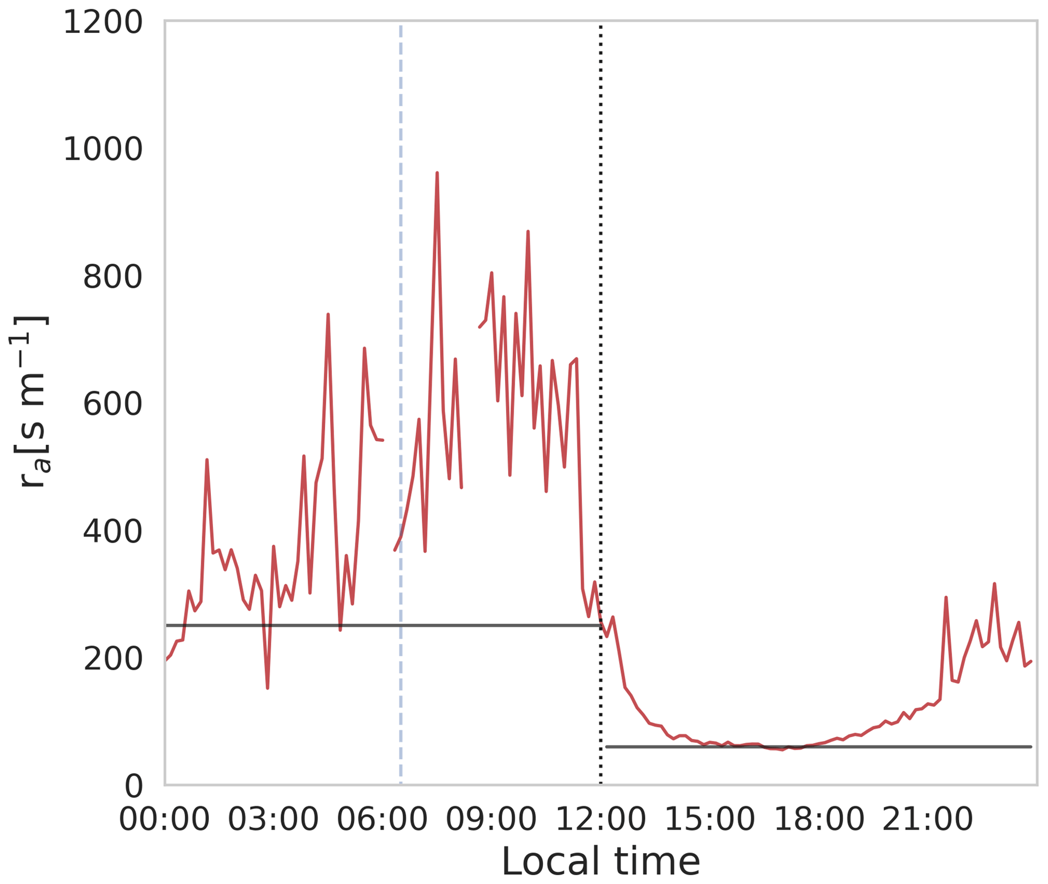
Figure A2Diurnal averaged aerodynamic resistance observed above the water surface during the E-DATA, and the black lines are the prescribed values under calm and windy regimes.
The saturated vapor pressure, es, which is also required in the aerodynamic contribution term, is approximated using the August–Roche–Magnus equation (Moene and Van Dam, 2014):
where Tak [K] is the absolute air temperature obtained from the ERA5 downscaled data, and a and b are 17.625 and −30.03, respectively.
A3 Energy balance non-closure coefficient
Since the Penman equation assumes energy balance closure and the E-DATA field data show a significant energy imbalance (Suárez et al., 2020), we introduce an energy balance non-closure coefficient, cEBNC, to correct the observed imbalance, which is the regression slope (m). Hence, this coefficient corrects the available energy to improve the energy balance closure. We observe two different non-closure balances that depend on the wind regime (Fig. A3). Therefore, we set cEBNC=0.3 for U<0.3 m s−1 (calm regime during the morning) and cEBNC=0.7 for U>3 m s−1 (windy regime during the afternoon).
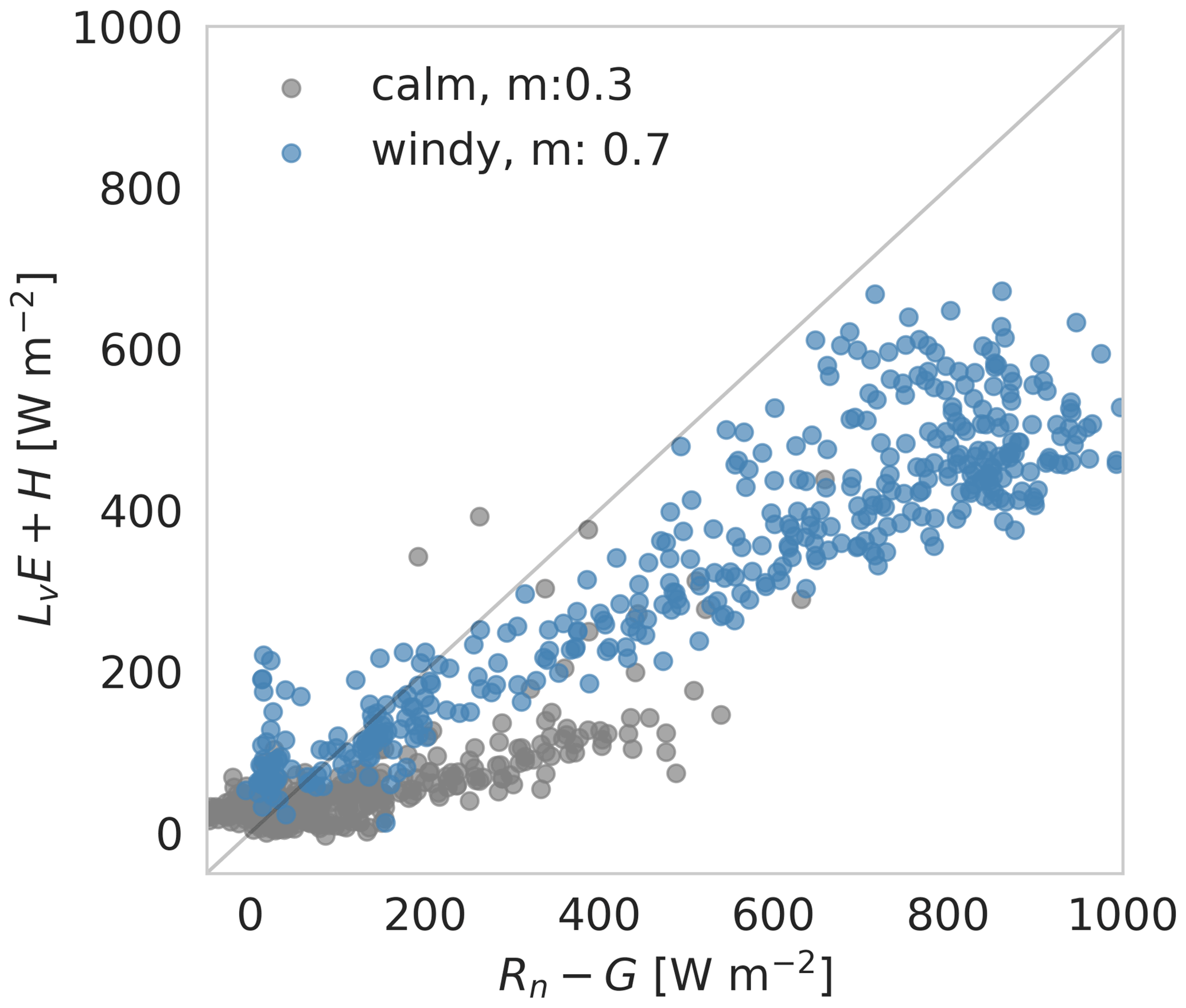
Figure A3Surface energy balance observed at the water surface during the E-DATA under calm and windy regimes; m corresponds to the regression slope.
Table A1Categorization of freezing hours and the ice coefficient.
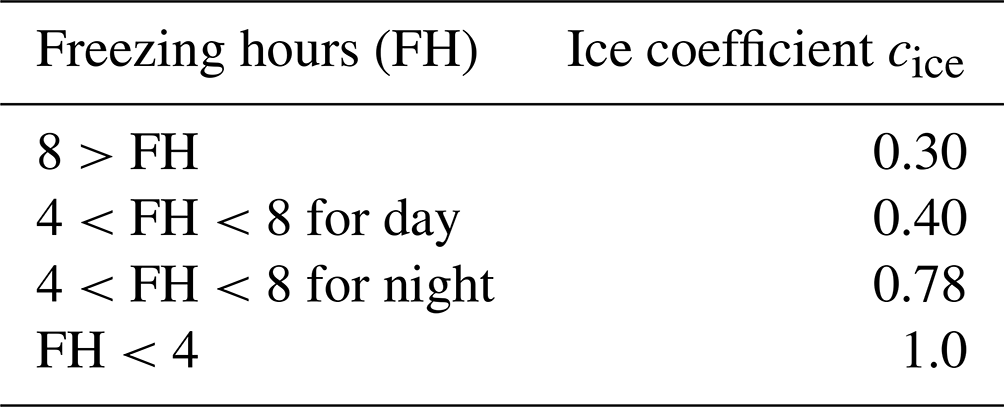
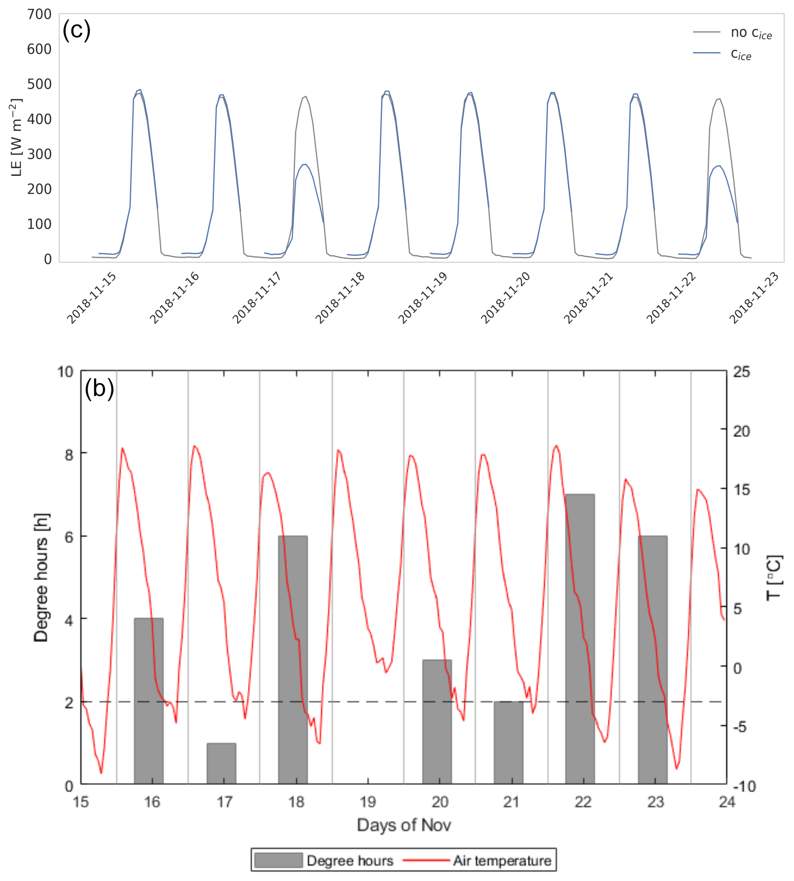
Figure A4(a) The effect of the ice coefficient on the site-adapted Penman evaporation estimates. (b) Degree hours and air temperature time series.
A4 Ice coefficient
Ice formation significantly restricts evaporation because it isolates the water from the atmosphere below a thin ice cover. Then, in the absence of wind, the available energy is used first to melt the ice before water evaporation occurs. Vergara-Alvarado (2017) demonstrated that a ∼3–5 cm thick ice cover in the SDH saline lake reduced the turbulent fluxes to zero by creating an isolating layer between the water surface and the atmosphere. Thus, neglecting ice formation leads to an overestimation of the latent heat flux. A complete ice model requires the derivation of heat transfer fluxes or an elaborated parameterization using variables and parameters that usually are not available in standard meteorological datasets (Echeverría et al., 2020). For this reason, we use an ice coefficient, cice, which ranges between 0 and 1, depending on the number of freezing hours per day (Table A1). The days are taken from midday to midday to include the night. The idea is that ice produced over longer periods takes longer to melt. We assumed that freezing occurs when the 2 m air temperature is below 270 K, slightly below the freezing temperature of clean water to include the effect of salinity. Based on this criterion, freezing days are distributed over the year as 6 % in summer, 21 % in autumn, 41 % in winter and 31 % in spring. Figure A4 shows the effect that the ice coefficient has in estimating latent heat flux during freezing days together with a time series of the freezing hours during the E-DATA.
Data are available at https://doi.org/10.17632/c5s6zk2rmz.2 (Lobos-Roco et al., 2020).
The article was written by FLR with the assistance of OH, JVGdA and FS. The data were analyzed by FLR and FS, who mainly contributed to ANN data processing. AH collaborated in Eq. (1) (Appendix A); IB collaborated in Sect. 3.2.1 (Fig. 7); AdlF provided the data used in Sect. 3.2.2 (Fig. 9).
The contact author has declared that neither they nor their co-authors have any competing interests.
Publisher's note: Copernicus Publications remains neutral with regard to jurisdictional claims in published maps and institutional affiliations.
This research received financial support from the Chilean National Commission of Science and Technology through the project ANID/FONDECYT/1210221. Support for Felipe Lobos-Roco was provided by the Wageningen University PhD Sandwich Project no.: 5160957644. Francisco Suárez acknowledges support from the Centro de Desarrollo Urbano Sustentable (CEDEUS – ANID/FONDAP/15110020) and from the Centro de Excelencia en Geotermia de los Andes (CEGA – ANID/FONDAP/15090013). Finally, we acknowledge Robin Palmer (English editing) and the two reviewers, Stephanie Kampf and Claudia Voigt, for their valuable contributions to this manuscript.
This research has been supported by the Fondo Nacional de Desarrollo Científico y Tecnológico (grant no. 1210221).
This paper was edited by Jan Seibert and reviewed by Stephanie Kampf and Claudia Voigt.
Aceituno, P.: On the functioning of the Southern Oscillation in the South American sector. Part I: Surface climate, Mon. Weather Rev., 116, 505–524, 1988. a, b, c, d
Aceituno, P.: El Niño, the Southern Oscillation, and ENSO: Confusing names for a complex ocean–atmosphere interaction, B. Am. Meteorol. Soc., 73, 483–485, 1992. a
Blin, N., Hausner, M., Leray, S., Lowry, C., and Suárez, F.: Potential Impacts of climate change on an aquifer in the arid Altiplano, northern Chile: the case of the protected wetlands of the Salar del Huasco basin, Journal of Hydrology: Regional Studies, 39, 100996, https://doi.org/10.1016/j.ejrh.2022.100996, 2022. a, b, c, d, e, f, g, h
Böhm, C., Reyers, M., Schween, J. H., and Crewell, S.: Water vapor variability in the Atacama Desert during the 20th century, Global Planet. Change, 190, 103192, https://doi.org/10.1016/j.gloplacha.2020.103192, 2020. a, b
Crawford, T. M. and Duchon, C. E.: An improved parameterization for estimating effective atmospheric emissivity for use in calculating daytime downwelling longwave radiation, J. Appl. Meteorol., 38, 474–480, 1999. a
Dee, D. P., Uppala, S. M., Simmons, A. J., Berrisford, P., Poli, P., Kobayashi, S., Andrae, U., Balmaseda, M. A., Balsamo, G., Bauer, P., Bechtold, P., Beljaars, A. C. M., van de Berg, L.,Bidlot, J., Bormann, N., Delsol, C., Dragani, R., Fuentes, M., Geer, A. J., Haimberger, L., Healy, S. B., Hersbach, H., Holm, E. V., Isaksen, L., Ållberg, P. K , Kohler, M., Matricardi, M., McNally, A. P., Monge-Sanz, B. M., Morcrette, J.-J., Park, B.-K., Peubey, C.,de Rosnay, P., Tavolato, C., Thepaut, J.-N., and Vitart, F.: The ERA-Interim reanalysis: Configuration and performance of the data assimilation system, Q. J. Roy. Meteor. Soc., 137, 553–597, 2011. a, b, c
de la Fuente, A.: Heat and dissolved oxygen exchanges between the sediment and water column in a shallow salty lagoon, J. Geophys. Res.-Biogeo., 119, 1129–1146, 2014. a
de la Fuente, A. and Meruane, C.: Spectral model for long-term computation of thermodynamics and potential evaporation in shallow wetlands, Water Resour. Res., 53, 7696–7715, 2017. a, b, c, d
de la Fuente, A., Meruane, C., and Suarez, F.: Long-term spatiotemporal variability in high Andean wetlands in northern Chile, Sci. Total Environ., 756, 143830, https://doi.org/10.1016/j.scitotenv.2020.143830, 2021. a, b, c, d
del Río, C., Lobos-Roco, F., Latorre, C., Koch, M. A., García, J.-L., Osses, P., Lambert, F., Alfaro, F., and Siegmund, A.: Spatial distribution and interannual variability of coastal fog and low clouds cover in the hyperarid Atacama Desert and implications for past and present Tillandsia landbeckii ecosystems, Plant Syst. Evol., 307, 1–23, 2021. a
Dibike, Y. B. and Coulibaly, P.: Temporal neural networks for downscaling climate variability and extremes, Neural Networks, 19, 135–144, 2006. a
Dorador, C., Vila, I., Witzel, K.-P., and Imhoff, J. F.: Bacterial and archaeal diversity in high altitude wetlands of the Chilean Altiplano, Fund. Appl. Limnol., 182, 135–159, 2013. a
Echeverría, S., Hausner, M. B., Bambach, N., Vicuña, S., and Suárez, F.: Modeling present and future ice covers in two Antarctic lakes, J. Glaciol., 66, 11–24, 2020. a
Falvey, M. and Garreaud, R. D.: Moisture variability over the South American Altiplano during the South American low level jet experiment (SALLJEX) observing season, J. Geophys. Res.-Atmos., 110, 1–12, 2005. a, b, c
Falvey, M. and Garreaud, R. D.: Regional cooling in a warming world: Recent temperature trends in the southeast Pacific and along the west coast of subtropical South America (1979–2006), J. Geophys. Res.-Atmos., 114, D04102, https://doi.org/10.1029/2008JD010519, 2009. a
Garreaud, R. and Aceituno, P.: Interannual rainfall variability over the South American Altiplano, J. Climate, 14, 2779–2789, 2001. a, b, c
Garreaud, R., Vuille, M., and Clement, A. C.: The climate of the Altiplano: observed current conditions and mechanisms of past changes, Palaeogeogr. Palaeocl., 194, 5–22, 2003. a, b, c
Hersbach, H., Bell, B., Berrisford, P., Hirahara, S., Horányi, A., Muñoz-Sabater, J., Nicolas, J., Peubey, C., Radu, R., Schepers, D., Simmons, A., Soci, C., Abdalla, S., Abellan, X., Balsamo, G., Bechtold, P., Biavati, G., Bidlot, J., Bonavita, M., De Chiara, G., Dahlgren, P., Dee, D., Diamantakis, M., Dragani, R., Flemming, J., Forbes, R., Fuentes, M., Geer, A., Haimberger, L., Healy, S., Hogan, R.-J., Hólm, E., Janisková, M., Keeley, S., Laloyaux, P., Lopez, P., Lupu, C., Radnoti, G., de Rosnay, P., Rozum, I., Vamborg, F., Villaume, S., and Thépaut, J.-N.: The ERA5 global reanalysis, Q. J. Roy. Meteor. Soc., 146, 1999–2049, 2020. a, b, c, d
Holtslag, A. and Van Ulden, A.: A simple scheme for daytime estimates of the surface fluxes from routine weather data, J. Appl. Meteorol. Clim., 22, 517–529, 1983. a
Houston, J.: Evaporation in the Atacama Desert: An empirical study of spatio-temporal variations and their causes, J. Hydrol., 330, 402–412, 2006. a, b, c, d, e, f
Huerta-Viso, A.: Estimating evaporation of a salt lake in the Atacama Desert with standard meteorological station data, MS thesis, Wageningen University & Research, Wageningen, the Netherlands, 2021. a
Jayne, R. S., Pollyea, R. M., Dodd, J. P., Olson, E. J., and Swanson, S. K.: Spatial and temporal constraints on regional-scale groundwater flow in the Pampa del Tamarugal Basin, Atacama Desert, Chile, Hydrogeol. J., 24, 1921–1937, 2016. a
Johnson, E., Yáñez, J., Ortiz, C., and Muñoz, J.: Evaporation d'eaux souterraines peu profoundes dans des bassins endoreiques de I'Altiplano Chilien, Hydrolog. Sci. J., 55, 624–635, 2010. a, b
Kampf, S. K., Tyler, S. W., Ortiz, C. A., Muñoz, J. F., and Adkins, P. L.: Evaporation and land surface energy budget at the Salar de Atacama, Northern Chile, J. Hydrol., 310, 236–252, 2005. a, b, c, d
Kumar, A. and Wen, C.: An oceanic heat content–based definition for the pacific decadal oscillation, Mon. Weather Rev., 144, 3977–3984, 2016. a
Kumar, J., Brooks, B.-G. J., Thornton, P. E., and Dietze, M. C.: Sub-daily statistical downscaling of meteorological variables using neural networks, Procedia Comput. Sci., 9, 887–896, 2012. a
Lictevout, E., Maass, C., Córdoba, D., Herrera, V., and Payano, R.: Recursos Hídricos de la Región de Tarapacá – diagnóstico y sistematización de la información, https://snia.mop.gob.cl/repositoriodga/handle/20.500.13000/4331 (last access: 14 April 2021), ISBN 978 956 302 081-6, 2013. a
Lobos-Roco, F., Vilà-Guerau de Arellano, J., and Pedruzo-Bagazgoitia, X.: Characterizing the influence of the marine stratocumulus cloud on the land fog at the Atacama Desert, Atmos. Res., 214, 109–120, 2018. a
Lobos Roco, F., Hartogensis, O., Vila, J., de la Fuente, A., and Suarez, F.: Dataset of Local evaporation controlled by regional atmospheric circulation in the Altiplano of the Atacama Desert, V2, Mendeley Data [data set], https://doi.org/10.17632/c5s6zk2rmz.2, 2020. a, b
Lobos-Roco, F., Hartogensis, O., Vilà-Guerau de Arellano, J., de la Fuente, A., Muñoz, R., Rutllant, J., and Suárez, F.: Local evaporation controlled by regional atmospheric circulation in the Altiplano of the Atacama Desert, Atmos. Chem. Phys., 21, 9125–9150, https://doi.org/10.5194/acp-21-9125-2021, 2021. a, b, c, d, e, f, g, h, i, j, k, l, m, n, o, p, q, r
Lobos-Roco, F., Hartogensis, O., Vilà-Guerau de Arellano, J., Aguirre, F., de la Fuente, A., and Suárez, F.: Optical-Microwave Scintillometer Evaporation measurements over a Saline Lake in a Heterogeneous Setting in the Atacama Desert, J. Hydrometeorol., 23, 909–924, https://doi.org/10.1175/JHM-D-21-0100.1, 2022. a, b, c
Moene, A. F. and Van Dam, J. C.: Transport in the atmosphere-vegetation-soil continuum, Cambridge University Press, ISBN 978-0-521-19568-3, 2014. a
Penman, H.: Natural evaporation from open water, bare soil and grass, P. Roy. Soc. Lond. A Mat., 193, 120–145, 1948. a, b, c, d
Rosen, M. R.: The importance of groundwater in playas: A review of playa classifications, The Geological Society of America, https://doi.org/10.1130/SPE289-p1, 1994. a
Rutllant, J., Fuenzalida, H., and Aceituno, P.: Climate dynamics along the arid northern coast of Chile: The 1997–1998 Dinámica del Clima de la Región de Antofagasta (DICLIMA) experiment, J. Geophys. Res.-Atmos., 108, 1–13, 2003. a, b, c
Scheihing, K. W., Moya, C. E., Struck, U., Lictevout, E., and Tröger, U.: Reassessing hydrological processes that control stable isotope tracers in groundwater of the Atacama Desert (Northern Chile), Hydrology, 5, 3, 2017. a
Suárez, F., Lobos-Roco, F., de la Fuente, A., Vilà-Guerau de Arellano, J., Prieto, A., Meruane, C., and Hartogensis, O.: E-DATA: A comprehensive field campaign to investigate evaporation enhanced by advection in the hyper-arid Altiplano, Water, 12, 745, 2020. a, b, c, d, e, f, g, h, i, j, k, l, m, n, o, p
Sugita, M. and Brutsaert, W.: Cloud effect in the estimation of instantaneous downward longwave radiation, Water Resour. Res., 29, 599–605, 1993. a, b
Timmermann, A., An, S., Kug, J.-S., Jin, F.-F., Cai, W., Capotondi, A., Cobb, K.-M., Lengaigne, M., McPhaden, M.-J., Stuecker, M.-F., Stein, K., Wittenberg, A.-T., Yun, K.-S., Bayr, T., Chen, H.-C., Chikamoto, Y., Dewitte, B., Dommenget, D., Grothe, P., Guilyardi, E., Ham, Y.-G., Hayashi, M., Ineson, S., Kang, D., Kim, S., Kim, W., Lee, J.-Y., Li, T., Luo, J.-J., McGregor, S., Planton, Y., Power, S., Rashid, H., Ren, H.-L., Santoso, A., Takahashi, K., Todd, A., Wang, G., Wang, G., Xie, R., Yang, W.-H., Yeh, S.-W., Yoon, J., Zeller, E., and Zhang, X.: El Niño–southern oscillation complexity, Nature, 559, 535–545, 2018. a
Uribe, J., Munoz, J. F., Gironas, J., Oyarzun, R., Aguirre, E., and Aravena, R.: Assessing groundwater recharge in an Andean closed basin using isotopic characterization and a rainfall-runoff model: Salar del Huasco basin, Chile, Hydrogeol. J., 23, 1535–1551, 2015. a, b, c, d, e, f, g
van der Ent, R. J.: A new view on the hydrological cycle over continents, PhD Thesis, TU Delft, Delft, ISBN 9789461824721, 2014. a, b
van der Ent, R. J., Savenije, H. H., Schaefli, B., and Steele-Dunne, S. C.: Origin and fate of atmospheric moisture over continents, Water Resour. Res., 46, W09525, https://doi.org/10.1029/2010WR009127, 2010. a, b
Vergara-Alvarado, J.: Estudio de la variabilidad intradiaria de los flujos de calor, masa y moméntum en la interfaz aire-agua de una laguna somera salina del Altiplano chileno, Universidad de Chile, http://repositorio.uchile.cl/handle/2250/146416 (last access: 9 January 2018), 2017. a, b
Voigt, C., Herwartz, D., Dorador, C., and Staubwasser, M.: Triple oxygen isotope systematics of evaporation and mixing processes in a dynamic desert lake system, Hydrol. Earth Syst. Sci., 25, 1211–1228, https://doi.org/10.5194/hess-25-1211-2021, 2021. a
Vuille, M., Bradley, R. S., and Keimig, F.: Interannual climate variability in the Central Andes and its relation to tropical Pacific and Atlantic forcing, J. Geophys. Res.-Atmos., 105, 12447–12460, 2000. a, b, c, d