How well are we able to close the water budget at the global scale?

The water budget equation describes the exchange of water between the land, ocean, and atmosphere. Being able to adequately close the water budget gives confidence in our ability to model and/or observe the spatio-temporal variations in the water cycle and its components. Due to advances in observation techniques, satellite sensors, and modelling, a number of data products are available that represent the components of water budget in both space and time. Despite these advances, closure of the water budget at the global scale has been elusive.

In this study, we attempt to close the global water budget using precipitation, evapotranspiration, and runoff data at the catchment scale. The large number of recent state-of-the-art datasets provides a new evaluation of well-used datasets. These estimates are compared to terrestrial water storage (TWS) changes as measured by the Gravity Recovery And Climate Experiment (GRACE) satellite mission. We investigated 189 river basins covering more than 90 % of the continental land area. TWS changes derived from the water balance equation were compared against GRACE data using two metrics: the Nash–Sutcliffe efficiency (NSE) and the cyclostationary NSE. These metrics were used to assess the performance of more than 1600 combinations of the various datasets considered.

We found a positive NSE and cyclostationary NSE in 99 % and 62 % of the basins examined respectively. This means that TWS changes reconstructed from the water balance equation were more accurate than the long-term (NSE) and monthly (cyclostationary NSE) mean of GRACE time series in the corresponding basins. By analysing different combinations of the datasets that make up the water balance, we identified data products that performed well in certain regions based on, for example, climatic zone. We identified that some of the good results were obtained due to the cancellation of errors in poor estimates of water budget components. Therefore, we used coefficients of variation to determine the relative quality of a data product, which helped us to identify bad combinations giving us good results. In general, water budget components from ERA5-Land and the Catchment Land Surface Model (CLSM) performed better than other products for most climatic zones. Conversely, the latest version of CLSM, v2.2, performed poorly for evapotranspiration in snow-dominated catchments compared, for example, with its predecessor and other datasets available. Thus, the nature of the catchment dynamics and balance between components affects the optimum combination of datasets. For regional studies, the combination of datasets that provides the most realistic TWS for a basin will depend on its climatic conditions and factors that cannot be determined a priori. We believe that the results of this study provide a road map for studying the water budget at catchment scale.

1 Introduction

A better understanding of hydrological processes at the catchment scale has been highlighted as one of the key challenges for hydrologists in the 21st century (Blöschl et al., 2019). One of the key processes is the terrestrial water cycle which can be described by the water balance equation:

$$\begin{array}{}\text{(1)}& {\displaystyle \frac{\mathrm{dTWS}}{\mathrm{d}t}}=P-\mathrm{ET}-R.\end{array}$$

This equation expresses the total amount of water gained by a river catchment in the form of precipitation (P) as the sum of water returning back to the atmosphere through evapotranspiration (ET), water flowing out of the catchment in the form of runoff (R), and any changes in the terrestrial water storage (TWS). TWS is defined as the sum of water stored as snow, canopy, soil moisture, groundwater, and surface water (Scanlon et al., 2018). The water balance equation is a budget equation that follows the conservation of mass, and it is an indispensable tool for validating our understanding of the catchment-scale water cycle.

Several studies have used the water balance equation to explain the hydro-climatic changes experienced in a river catchment (e.g. Landerer et al., 2010; Pan et al., 2012; Oliveira et al., 2014; Saemian et al., 2020), to validate modelled estimates of one component (e.g. Bhattarai et al., 2019; Long et al., 2015; Wan et al., 2015), or to estimate one component when others are known (Chen et al., 2020; Gao et al., 2010; Wang et al., 2014). It should be noted, however, that the accuracy of the result in these studies is limited by uncertainties associated with individual components. For example, Sahoo et al. (2011) attempted to close the water balance equation for 10 large catchments and found that the imbalance error amounted to up to 25 % of mean annual precipitation. Additionally, Zhang et al. (2018) highlighted the source of the imbalance error as being predominantly from stark disagreement between evapotranspiration estimates.

Obtaining high-quality spatio-temporal estimates of components of the water balance is challenging due to a lack of global in situ measurement networks and political will to sustain any existing network. Therefore, the era of satellite remote sensing offers an excellent solution to monitoring the hydrosphere. With the help of dedicated satellite missions, we are able to measure variables that can be used to estimate water balance components. However, monitoring TWS has been the most difficult part because it includes water on and below the surface of the Earth, and optical remote sensing can only offer information near the surface. This issue was solved by the launch of the Gravity Recovery And Climate Experiment (GRACE) satellite gravimetry mission from the German GeoForschungsZentrum (GFZ) and the National Aeronautics and Space Administration (NASA) in 2002 (Wahr et al., 1998; Tapley, 2004). This mission measures the temporal variations in the Earth's gravity field, which can then be related to water mass change on and below the surface of the Earth. GRACE provides the most accurate global estimations of TWS to date, which can be used in the water balance equation (Eq. 1).

Another challenge concerns components like ET with a high spatial variability, which requires precise satellite estimates that are not consistently available due to observational constraints (Fisher et al., 2017). As ET accounts for up to 60 % of precipitation in some regions, it is a crucial component of the water cycle (Oki and Kanae, 2006). It also constitutes the most significant uncertainties of the terrestrial water cycle components (Rodell et al., 2015). The water balance equation has been used to compensate for this lack of knowledge and increase our understanding of ET. Water budget studies have generally found that ET inferred from the water balance equation agrees well with remote sensing estimates in terms of seasonal cycle but presents larger inter-annual variability (Liu et al., 2016; Pascolini-Campbell et al., 2020; Swann and Koven, 2017) and larger magnitudes (Bhattarai et al., 2019; Long et al., 2014; Wan et al., 2015).

Apart from ET, our knowledge of R also benefits from water budget estimations. Although river discharge can be measured by gauges, the spatio-temporal coverage of in situ measurements is limited due to a lack of resources in some regions and political will to share data. Uncertainties and biases in P have been found to be the main drivers of the inaccuracy in budget-inferred R (Sheffield et al., 2009; Oliveira et al., 2014; Sneeuw et al., 2014; Wang et al., 2014; Xie et al., 2019). Water budget studies using R as a reference variable also point out the difficulty involved in finding datasets able to close the water budget (Chen et al., 2020; Gao et al., 2010; Lorenz et al., 2014). Moreover, ET and R are strongly intertwined, and accurate estimates of one cannot be achieved without a better constraint on the other (Armanios and Fisher, 2014; Lv et al., 2017; Penatti et al., 2015).

To improve the reliability of available data, the water budget can be used as a discriminating tool to assess the accuracy of various datasets. For this to be achieved, there is a need to first evaluate the water budget closure globally, including basins of all sizes and comparing as many state-of-the-art datasets as possible. This review is currently lacking because a majority of studies have concentrated only on a few selected basins with specific climatic conditions (e.g. the Amazon Basin – Swann and Koven, 2017; Chen et al., 2020) or basins highly impacted by human activities (e.g. the Yellow River basin – Lv et al., 2017; Long et al., 2015). Additionally, the studies that look at several basins worldwide have only evaluated sparsely distributed basins, which leaves entire zones without analysis (Sahoo et al., 2011; Pan et al., 2012; Lorenz et al., 2014; Liu et al., 2016; Zhang et al., 2018). This has deprived hydrologists of a comprehensive global overview of the water budget.

Returning to the requirement for basins of all sizes, basins were also generally chosen to be quite large in the majority of studies. It is known that the accuracy of GRACE measurements is directly proportional to the size of the basin (Rodell and Famiglietti, 1999; Wahr et al., 2006; Vishwakarma et al., 2018); however, the lower limit of ∼200 000 km² established by Longuevergne et al. (2010), which has long been used, is no longer a requirement to retrieve GRACE signals. It has been shown that basins as small as ∼70 000 km² can be precisely recovered by GRACE measurements and that their size do not influence the closure of the water budget (Gao et al., 2010; Lorenz et al., 2014; Vishwakarma et al., 2018). Therefore, they are included in the current study.

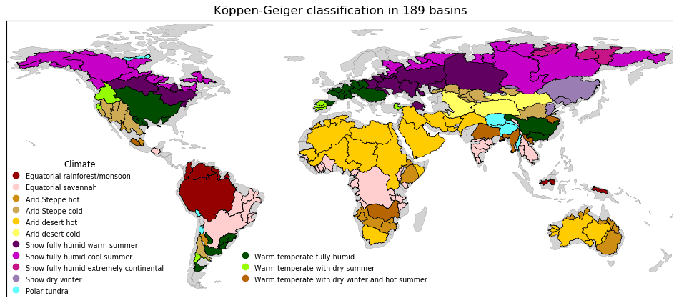
Figure 1 The 189 basins larger than 63 000 km² with their corresponding climate zone.

Regarding the number of datasets to be examined, each water budget study uses different datasets, some of which were available only over a given continent or over short time periods. To the authors' best knowledge, Lorenz et al. (2014) conducted the study comparing the largest number of datasets by assessing more than 180 combinations of P, ET, and TWS datasets. However, many datasets have since improved, especially reanalyses such as ERA-Interim (Dee et al., 2011) and MERRA-Land (Reichle et al., 2011). It would be beneficial to provide an updated evaluation of those widely used datasets.

Thus, the aim of the current study is to provide a revised overview of the water budget closure on a global scale. Section 2 presents the study area covering all parts of the globe (excluding Greenland and Antarctica) and the datasets. Section. 3 then details the metrics used to evaluate the water budget closure as well as the selection process for the best combinations. Finally, Sect. 4 explains the results and discusses previous studies.

2 Data

2.1 Study area

We used the major river basins from the Global Runoff Data Centre (GRDC, 2020) to define the study area. As the spatial resolution of GRACE products for hydrological applications is around 63 000 km² (Vishwakarma et al., 2018), catchments larger than this limit have been included in our analysis. Furthermore, these basins were assigned to a climate zone as defined by the Köppen–Geiger classification (Kottek et al., 2006). The 189 basins under study are depicted in Fig. 1, and their areas range from ∼65 600 to ∼5 965 900 km².

2.2 Datasets

We have used freely available global state-of-the-art datasets with a temporal resolution smaller than or equal to 1 month and coverage of at least 2003 to 2014. If necessary, data have been interpolated to $\mathrm{0.5}{}^{\circ }\times \mathrm{0.5}{}^{\circ }$ grids using bilinear interpolation to correspond with monthly TWS derived from the GRACE satellite mission. In this study, GRACE mascon fields were obtained from the Jet Propulsion Laboratory (JPL) Release 06 (RL06) (Watkins et al., 2015; Wiese et al., 2018). Our results were also computed with mascons from the Center for Space Research (CSR) and can be easily reproduced with the code that we provide. As this did not significantly changed our findings, we only show results using JPL mascons.

For other variables, daily data were aggregated to monthly values taking the number of days per month into account. Finally, gridded data were weighted by the area of each grid cell and then aggregated over a basin to obtain a time series.

2.2.1 Precipitation datasets

Precipitation data were obtained from various sources that are summarised in Table S1 in the Supplement. Three datasets rely only on rain-gauge measurements, namely the Climate Research Unit (CRU), which uses around 10 000 gauges (Harris et al., 2020); the Global Unified Gauge-Based Analysis of Daily Precipitation from the Climate Prediction Center (CPC), which is based on approximately 30 000 gauges (Chen and Xie, 2008); and the Global Precipitation Climatology Centre (GPCC), which maintains a database of around 67 000 gauges (Schneider et al., 2020). Surface observations are often used to calibrate satellite estimations or as input variables in reanalyses. As the global coverage of rain gauges is not homogeneous, the quality of such products varies regionally; thus, satellite-based products provide a good alternative.

Two satellite missions were specifically designed to measure precipitation. The Tropical Rainfall Measuring Mission (TRMM) operated from 1998 to 2015 and provided monthly estimations of precipitation over the region from 50^∘ N to 50^∘ S. We used the TRMM Multi-satellite Precipitation Analysis (TMPA) 3B43 version that extends TRMM measurements until 2020 via calibration with other satellites (Huffman et al., 2007, 2010). The Global Precipitation Measurement (GPM) mission was built on TRMM findings since its launch in February 2014. This constellation of satellites is calibrated using previous satellites through the Integrated Multi-satellitE Retrievals for GPM (IMERG) to provide global coverage from 2000 onwards (Huffman et al., 2019). Finally, the Global Precipitation Climatology Project (GPCP) merges various satellite-based estimates with rain-gauge measurements from the GPCC (Adler et al., 2018). It provides a well-used and long dataset spanning from 1979 to the present.

Apart from these, reanalyses products provide consistent estimations of precipitation, evapotranspiration, and runoff. ERA5-Land is a rerun of the land component from the ERA5 reanalysis developed by the European Centre for Medium-Range Weather Forecasts (ECMWF). Precipitation data are obtained from satellite measurements including but not restricted to TRMM and GPM results and are provided from 1981 onwards (Muñoz‐Sabater, 2019). The Japanese 55-year Reanalysis (JRA-55) also derives precipitation from satellite measurements with forecasts starting in 1958 (Kobayashi et al., 2015). Finally, the Modern-Era Retrospective Analysis for Research and Applications, version 2 (MERRA-2) uses two precipitation datasets from the CPC: the Global Unified Gauge-Based Analysis of Daily Precipitation described above and the Merged Analysis of Precipitation which combines gauge-based and satellite measurements (Reichle et al., 2017).

Finally, two additional datasets that combine rain-gauge observations, satellite measurements, and reanalyses were used in this study: the Princeton Global Forcing (PGF) dataset and the Multi-Source Weighted Ensemble Precipitation (MSWEP) dataset. PGF was included as it is one of the forcing variables used in the Global Land Data Assimilation System (GLDAS) (Sheffield et al., 2006). Recently developed, MSWEP merges gauge observations (including GPCC), satellite measurements (including TRMM), and reanalyses (ERA-Interim and JRA-55) (Beck et al., 2019).

As there are large disagreements between different datasets, it is important to assess whether a dataset is in general agreement with others. By revealing datasets with significant bias, this method can limit the occurrence of error cancellation, which is a well-known problem in water budget studies (Sneeuw et al., 2014; Lorenz et al., 2014). We have used the coefficient of variation (CV) to evaluate various datasets of a water budget component in each basin. From a group of datasets, the CV is a time series defined as the standard deviation divided by the mean. (A minimum value of 10 mm was enforced for the mean to avoid high CVs during the dry season.) The higher the CV, the greater the disagreement between datasets. Figure S1 in the Supplement shows the mean of the CV time series in each basin. Unsurprisingly, satellite datasets (TRMM, GPM, and GPCP) provide close results because they use similar measurements and are, therefore, not at all independent. Observations datasets (CPC, CRU, and GPCP) are more independent, which leads to higher CVs. However, apart from Australia, where CRU led to precipitation values that were consistently smaller than CPC and GPCC, there were no common patterns in the other regions. In addition, the major differences between reanalyses were found in Central Asia where MERRA2 gave much lower precipitation values than ERA5-Land and JRA-55. Interestingly, Fig. S1 also shows that the method used to create the dataset (i.e. rain-gauge observations, satellite measurements, or reanalyses) is less relevant than differences within a method. The inter-category CV measuring differences between the mean of observations, satellite, and reanalyses datasets was found to be relatively low. The highest CVs were found in high-latitude basins where reanalyses consistently led to higher precipitation values whereas observations had the lowest precipitation values.

2.2.2 Evapotranspiration datasets

Evapotranspiration is the sum of evaporation from water surfaces and transpiration through vegetation. Datasets used in this study are listed in Table S2. One of the most accurate methods to estimate evapotranspiration is the Penman–Monteith equation (Penman, 1948; Monteith, 1965). The variables used in this equation are obtained from various land surface parameterisations and energy balance equations in reanalyses, ERA5-Land and MERRA2, and in GLDAS land surface models (LSMs). We chose three variants of the GLDAS: the Variable Infiltration Capacity (VIC; Liang et al., 1994), the Noah model (Chen et al., 1996; Koren et al., 1999; Ek et al., 2003), and the Catchment Land Surface Model (CLSM; Koster et al., 2000). These LSMs are forced with different data depending on the GLDAS version (Rodell et al., 2004). For example, PGF precipitation was used in version 2.0, GPCP precipitation was used in version 2.1, and ERA5 precipitation was used in version 2.2 coupled with GRACE data assimilation (for CLSM only; Li et al., 2019). The MOD16 algorithm also uses the Penman–Monteith equation with measurements from the Moderate Resolution Imaging Spectroradiometer (MODIS, NASA) (Mu et al., 2011).

One of the main drawbacks of the Penman–Monteith equation is the reliance on a large number of parameters, such as vegetation characteristics, air temperature, wind, and vapour pressure. As these parameters can be difficult to assess accurately, alternative approaches have been developed. For example, the Global Land Evaporation Amsterdam Model (GLEAM) uses an equation involving fewer parameters, the Priestley–Taylor equation (Martens et al., 2017; Miralles et al., 2011). Another method relies on the energy budget to compute the fraction of energy leading to water vaporisation, as done in the Simplified Surface Energy Balance for operational applications (SSEBop) (Senay et al., 2013). Finally, algorithms also take advantage of the FLUXNET network of eddy-covariance towers measuring evapotranspiration. To this extent, the machine learning FLUXCOM algorithm (Jung et al., 2019) extends the methodology of the well-used Multi-Tree Ensemble (Jung et al., 2009) by exploiting relationships between meteorological variables and latent heat flux measured by eddy-covariance towers.

Similar to precipitation, Fig. S2 shows the coefficient of variation for different categories of evapotranspiration datasets. CVs were relatively low between the mean of all categories, as was found for precipitation. The largest differences between reanalyses were also found in Central Asia, with MERRA2 predicting lower evapotranspiration. In addition, it is striking to see the large CVs among land surface models (CLSM, Noah, and VIC with versions 2.0 and 2.1). In this category, there were consistent patterns across all basins with VIC tending to underestimate ET while CLSM provided slightly larger values. The CVs were especially large in high-latitude basins due to low ET in the cold season. Moreover, in Fig. S2, we see that the differences between remote sensing datasets (FLUXCOM, GLEAM, MOD16, and SSEBop) are not spatially consistent. In Australia, MOD16 led to significantly lower ET, especially during the hot season (October to February). In South Africa, differences were constant all year long, with MOD16 being lower while FLUXCOM was rather high. We do not comment on CVs in hot deserts (the Sahara, the Arabian Peninsula, and Central Asia) because FLUXCOM and MOD16 are not available in non-vegetated land areas.

2.2.3 Runoff datasets

Runoff is computed in LSMs as the excess water not evaporated from soils. This water infiltrates through the soil to the lowest layers without communicating with adjacent grid cells. All of the LSMs presented above provide runoff estimates that were included in this study. River discharge measurements are also available from gauge records, but they are not temporally consistent across the study period. In addition, discharge areas from the gauge stations with the longest records do not necessarily match the area of GRDC basins that we selected. Therefore, we decided to use only spatially and temporally consistent datasets by excluding gauge records from our analyses. However, we used the recently developed machine learning Global Runoff (GRUN) Reconstruction dataset which provides runoff values at a $\mathrm{0.5}{}^{\circ }\times \mathrm{0.5}{}^{\circ }$ spatial resolution from 1902 to 2014 (Ghiggi et al., 2019). This algorithm was trained with precipitation, temperature, and runoff measurements and validated against independent river discharge observations from the GRDC.

As for precipitation and evapotranspiration, Fig. S3 shows the coefficients of variation. CVs were generally higher for runoff than that for evapotranspiration and precipitation. Even though it reflects high uncertainties in runoff values, this should play a relatively smaller role in the water balance because the runoff is the smallest water cycle component. In Fig. S3, the inter-category CVs were computed between GRUN, the mean of LSMs, and the mean of reanalyses. The general observations are complementary to those made about evapotranspiration. VIC generally led to the highest values among all datasets. Reanalyses tended to be lower, along with CLSM. Finally, compared to the mean across all datasets, GRUN was relatively close in general (not shown). The largest differences were found in Australia and Central Africa, where GRUN was lower, as well as in Central Asia, where it led to higher values.

3 Methods

3.1 Water budget reconstruction

GRACE mascon fields were used to compute time series of TWS anomalies relative to the mean between 2004 and 2009. As Eq. (1) involves the variation of TWS over a time period, which is called the terrestrial water storage change (TWSC), to obtain TWSC from TWS anomalies, the time derivative was computed with centred finite difference (as in e.g. Long et al., 2014, or Pascolini-Campbell et al., 2020):

$$\begin{array}{}\text{(2)}& \mathrm{TWSC}\left(t\right)={\displaystyle \frac{\mathrm{TWS}(t+\mathrm{1})-\mathrm{TWS}(t-\mathrm{1})}{\mathrm{2}\mathrm{\Delta }t}},\end{array}$$

where Δt equals 1 month, and t−1, t, and t+1 are three consecutive months. Missing monthly values were filled with cubic interpolation. In order to match the temporal shift induced by the central difference, time series of P, ET, and R also needed to be time-filtered by Eq. (3) (Landerer et al., 2010):

$$\begin{array}{}\text{(3)}& \stackrel{\mathrm{̃}}{X}\left(t\right)={\displaystyle \frac{\mathrm{1}}{\mathrm{4}}}X(t-\mathrm{1})+{\displaystyle \frac{\mathrm{1}}{\mathrm{2}}}X\left(t\right)+{\displaystyle \frac{\mathrm{1}}{\mathrm{4}}}X(t+\mathrm{1}),\end{array}$$

where X denotes either P, ET, or R. All variables referred to hereafter are filtered variables but are denoted without the tilde notation for the sake of clarity.

Each triplet of datasets (data_P, data_ET, data_R) was called a combination and led to a budget reconstruction of TWSC computed with Eq. (1): ${\mathrm{TWSC}}_{\mathrm{budget}}\left(t\right)=P_{{\mathrm{data}}_{\mathrm{P}}}\left(t\right)-{\mathrm{ET}}_{{\mathrm{data}}_{\mathrm{ET}}}\left(t\right)-R_{{\mathrm{data}}_{\mathrm{R}}}\left(t\right)$. This reconstruction was compared with the derivatives obtained from Eq. (2) and denoted TWSC_GRACE(t). As we used 11 precipitation, 14 evapotranspiration, and 11 runoff datasets, we finally evaluated 1694 combinations.

3.2 Metrics

Differences between two time series are commonly evaluated with the root mean square deviation (RMSD):

$$\begin{array}{}\text{(4)}& \mathrm{RMSD}=\sqrt{{\displaystyle \frac{\mathrm{1}}{T}}\sum _{t=\mathrm{1}}^T{\left({\mathrm{TWSC}}_{\mathrm{budget}}\left(t\right)-{\mathrm{TWSC}}_{\mathrm{GRACE}}\left(t\right)\right)}^{\mathrm{2}}}.\end{array}$$

The main drawback of the RMSD is that it is not normalised (i.e. basins with large TWSC tend to have larger RMSD). A very common normalisation is the Nash–Sutcliffe efficiency (NSE) introduced by Nash and Sutcliffe (1970) to evaluate modelled runoff compared to observations:

$$\begin{array}{}\text{(5)}& \begin{array}{rl}\mathrm{NSE}& =\mathrm{1}-{\displaystyle \frac{\frac{\mathrm{1}}{T}\sum _{t=\mathrm{1}}^T{\left({\mathrm{TWSC}}_{\mathrm{budget}}\left(t\right)-{\mathrm{TWSC}}_{\mathrm{GRACE}}\left(t\right)\right)}^{\mathrm{2}}}{\frac{\mathrm{1}}{T}\sum _{t=\mathrm{1}}^T{\left({\mathrm{TWSC}}_{\mathrm{GRACE}}\left(t\right)-\stackrel{\mathrm{‾}}{{\mathrm{TWSC}}_{\mathrm{GRACE}}}\right)}^{\mathrm{2}}}}\\ & =\mathrm{1}-{\displaystyle \frac{{\mathrm{RMSD}}^{\mathrm{2}}}{{\mathit{\delta }}_{\mathrm{cst}}^{\mathrm{2}}}},\end{array}\end{array}$$

where $\stackrel{\mathrm{‾}}{{\mathrm{TWSC}}_{\mathrm{GRACE}}}=\frac{\mathrm{1}}{T}\sum _{t=\mathrm{1}}^T{\mathrm{TWSC}}_{\mathrm{GRACE}}\left(t\right)$ is the long-term mean of TWSC, and δ_cst is the deviation of monthly values from the long-term mean. In our case, any positive value of the NSE means that the budget reconstruction of TWSC_GRACE is a better approximation than the long-term mean. The maximum value of 1 describes a perfect reconstruction, and a negative value denotes poor performance. One major advantage of the NSE is that it requires both phase agreement (usually assessed with the correlation coefficient) and a small long-term mean error (evaluated with the bias or percentage bias) to yield high values (Lorenz et al., 2014).

However, although several attempts have been made to associate positive NSE values to performance (e.g. Henriksen et al., 2003; Samuelsen et al., 2015), it is known that this index suffers from several weaknesses; for example, a high positive NSE can be obtained with a poor time series if the time series has a large variance (Jain and Sudheer, 2008). In the context of the current study, basins with large seasonal variations of TWSC, especially tropical basins, are more likely to exhibit a NSE close to one even though the budget reconstruction presents substantial errors.

To overcome this issue, it has been proposed to compare the budget reconstruction to the mean monthly value of TWSC instead of comparing it to the constant long-term mean. The so-called cyclostationary NSE (Thor, 2013; Zhang, 2019) is then expressed as follows:

$$\begin{array}{}\text{(6)}& \begin{array}{rl}{\mathrm{NSE}}_{\mathrm{c}}& =\mathrm{1}-{\displaystyle \frac{\frac{\mathrm{1}}{T}\sum _{t=\mathrm{1}}^T{\left({\mathrm{TWSC}}_{\mathrm{budget}}\left(t\right)-{\mathrm{TWSC}}_{\mathrm{GRACE}}\left(t\right)\right)}^{\mathrm{2}}}{\frac{\mathrm{1}}{T}\sum _{t=\mathrm{1}}^T{\left({\mathrm{TWSC}}_{\mathrm{GRACE}}\left(t\right)-{\mathrm{TWSC}}_{\mathrm{GRACE}}^m\right)}^{\mathrm{2}}}}\\ & =\mathrm{1}-{\displaystyle \frac{{\mathrm{RMSD}}^{\mathrm{2}}}{{\mathit{\delta }}_{\mathrm{cyc}}^{\mathrm{2}}}},\end{array}\end{array}$$

where ${\mathrm{TWSC}}_{\mathrm{GRACE}}^m$ is the mean value for month m over all years, and δ_cyc is the deviation of GRACE TWSC from the periodic monthly signal. Similarly to the NSE, positive values of the cyclostationary NSE indicate a budget reconstruction better than the mean annual cycle, which measures the ability of the reconstruction to capture anomalous events (Lorenz et al., 2015; Tourian et al., 2017).

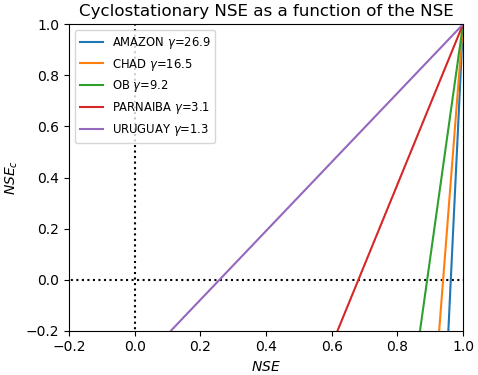
Moreover, one can express the cyclostationary NSE in terms of the NSE by combining Eqs. (5) and (6) as follows:

$$\begin{array}{}\text{(7)}& {\mathrm{NSE}}_{\mathrm{c}}=\left(\mathrm{1}-{\displaystyle \frac{{\mathit{\delta }}_{\mathrm{cst}}^{\mathrm{2}}}{{\mathit{\delta }}_{\mathrm{cyc}}^{\mathrm{2}}}}\right)+\underset{\mathit{\gamma }}{\underbrace{{\displaystyle \frac{{\mathit{\delta }}_{\mathrm{cst}}^{\mathrm{2}}}{{\mathit{\delta }}_{\mathrm{cyc}}^{\mathrm{2}}}}}}\mathrm{NSE}.\end{array}$$

The γ factor describes the behaviour of the TWSC by comparison with the mean seasonal cycle. Basins with periodic seasonal cycles (i.e. low δ_cyc) or large magnitudes (i.e. high δ_cst) have larger γ. In those basins (e.g. the Amazon or Chad basins), extremely high NSE values are required to achieve a positive cyclostationary NSE, as can be seen in Fig. 2. Special attention must then be given when examining such basins to discriminate performance depending on the NSE or the cyclostationary NSE.

Figure 2 The cyclostationary NSE is related to the NSE through ${\mathrm{NSE}}_{\mathrm{c}}=\mathrm{1}-\mathit{\gamma }+\mathit{\gamma }\mathrm{NSE}$, where $\mathit{\gamma }=\frac{{\mathit{\delta }}_{\mathrm{cst}}^{\mathrm{2}}}{{\mathit{\delta }}_{\mathrm{cyc}}^{\mathrm{2}}}$.

3.3 Selection of the most representative datasets

When estimating a water cycle component from the water balance equation (Eq. 1), it is useful to know beforehand which datasets are more reliable to close the water budget in the region under study. This section aims to describe how such datasets can be selected. The NSE results were stored in a matrix where each row corresponded to a basin and each column to a combination. Due to the matrix dimension (189×1694), an automated computation was needed to evaluate the combinations. This was achieved by introducing a cost function which represented the loss of accuracy when using any combination instead of the optimal one.

Our method can be summarised as follows:

1. compute the cost matrix to describe the performance of each combination;

2. cluster basins into larger zones depending on the similarities between cost vectors;

3. for each zone, select the combinations satisfying a maximum cost and extract the underlying datasets.

In more detail, the following steps were performed:

1. Using a cost function instead of the absolute metrics allowed us to overcome the lack of a NSE scale. On the one hand, there are significant differences between a combination leading to a budget reconstruction with a NSE close to 0 and another leading to an almost perfect reconstruction (NSE close to 1). These differences can be seen, for example, in terms of months where the budget reconstruction is within the confidence interval from GRACE TWSCs. Therefore, we want to favour combinations leading to the highest NSE values. On the other hand, one cannot determine a NSE threshold assuring a satisfying reconstruction in all basins. Figure 2 shows that very high NSE values were needed in basins with large γ to outperform the monthly periodic signal. Consequently, a cost function evaluates the performance of a combination relative to the largest NSE achievable in each basin. The cost function was then defined from the NSE by

   $$\begin{array}{}\text{(8)}& c_i^{\mathrm{b}}={\max }_{\mathrm{comb}}{\mathrm{NSE}}^{\mathrm{b}}\left(\mathrm{comb}\right)-{\mathrm{NSE}}^{\mathrm{b}}\left({\mathrm{combination}}_i\right),\end{array}$$

   where the maximum was computed over all 1694 combinations. We emphasise that the cost was evaluated independently for each basin (denoted by the superscript “b”), allowing the maximum NSE to be different in each basin. For combinations leading to a cost larger than 2 (i.e. a NSE below −1), the cost was restricted to 2. This limited the penalisation of combinations with highly negative values but had no major influence on our results because we focused on the best performing combinations.

2. From the cost matrix, each basin could be represented by a vector of 1694 costs. The similarities between two basins b₁ and b₂ were evaluated based on the Euclidean distance between their respective cost vector, $d(b_{\mathrm{1}},b_{\mathrm{2}})=\sqrt{\sum _{i=\mathrm{1}}^{\mathrm{1694}}(c_i^{b_{\mathrm{1}}}-c_i^{b_{\mathrm{2}}}{)}^{\mathrm{2}}}$. For two basins to have a small Euclidean distance, each combination i should lead to a similar cost in all basins: either the combination was satisfying in both cases ($c_i^{b_{\mathrm{1}}}\simeq \mathrm{0}$ and $c_i^{b_{\mathrm{2}}}\simeq \mathrm{0}$), or it did not perform well in both ($c_i^{b_{\mathrm{1}}}\simeq \mathrm{2}$ and $c_i^{b_{\mathrm{2}}}\simeq \mathrm{2}$). A hierarchical clustering algorithm was then applied to cluster basins so as to minimise the variance between cost vectors inside a cluster (Mueller et al., 2011).

3. Finally, the maximal cost for combinations to be considered as satisfying the water budget closure was chosen to be 0.1. This means that the difference between the RMSD of a suitable combination and the lowest RMSD over all combinations is, on average, lower than $A/\mathrm{10}$, where A is the mean seasonal amplitude of TWSC. This threshold guarantees that selected combinations a performance similar to the optimal combination. Then, in each cluster determined by the algorithm, we selected the combinations with a cost lower than 0.1 for all basins in the cluster. From the selected combinations, we extracted the underlying datasets of P, ET, and R. By reporting the number of combinations in which each dataset appeared, we could evaluate whether a dataset was clearly better than the others in a given region.

4 Results and discussion

4.1 Water budget closure

In order to assess the global water budget closure, we first examined the instances with the best performance across all combinations. This means that, for each basin, we reported the highest NSE among all 1694 combinations. Figure 3 shows the maximum NSE that can be achieved from a combination. Please note that a positive NSE was obtained over 99 % of the total study area. Only 9 basins out of 189 did not achieve a positive NSE for any combination. These were mainly hot arid deserts in the northern Sahara, Somalia, and Australia as well as two other basins in Papua New Guinea (Mamberamo Basin) and Canada (Hayes Basin) (Fig. 3). The poor performance in arid basins can be explained by limited precipitation and water storage variations that lead to a low signal-to-noise ratio. This is a major difference from previous studies where, for example, Lorenz et al. (2014) found that only 29 basins out of 96 achieved a positive NSE.

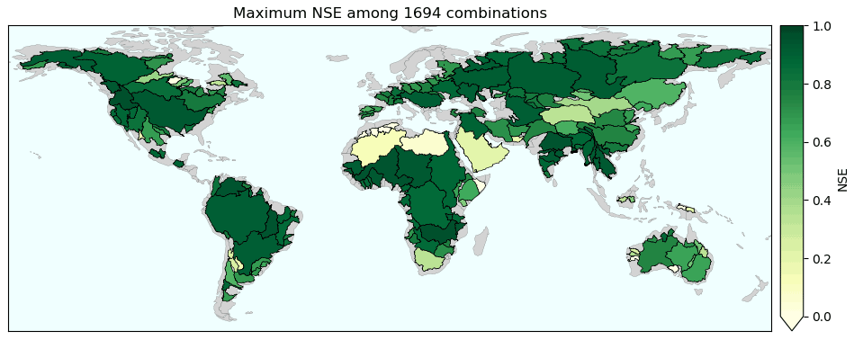
Figure 3 Maximum NSE per basin over all combinations. Green positive values mean that the budget reconstruction is a better approximation of GRACE TWSC than the long-term mean.

Figure 3 can be interpreted as follows: all of the basins with a positive NSE offer a budget reconstruction better than the long-term mean from GRACE TWSC. In addition, higher NSE values correspond to a better fit between reconstructed TWSC and GRACE TWSC. Figure S4 then shows the distribution of the maximum NSE. Although it has been explained (in Sect. 3.2) that positive NSE should be interpreted cautiously, one can observe that 61 % of the study area satisfied a NSE larger than 0.8, which is usually considered very good performance (e.g. Henriksen et al., 2003; Samuelsen et al., 2015). Given the large number of datasets, it is likely that cancellation of errors explains some of the instances with good performance. The reader should remain cautious about this possibility when trying to reproduce our results and may use discrepancy measures such as the CV to examine datasets, as explained in the following sections.

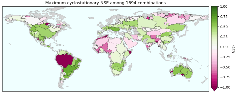
Figure 4 Maximum cyclostationary NSE per basin over all combinations. Green positive values mean that the budget reconstruction is a better approximation of GRACE TWSC than the mean monthly values.

By definition, the NSE can only be used to compare the budget reconstruction with the long-term mean. As predicting intra-annual variations of TWSC would be more beneficial for hydro-meteorological studies, the cyclostationary NSE was also used to assess the quality of reconstructed TWSC. Figure 4 shows that a positive maximum cyclostationary NSE was achieved over 62 % of the study area. It means that, in those basins, the reconstructed TWSC was better than the mean annual cycle obtained from GRACE TWSC. The budget reconstruction performed especially well in the continental United States (CONUS) and Central America, in most of South America except the Amazon and the Andes, and in southern Africa, Australia, Europe, western Russia, and East Asia (Fig. 4).

When comparing Figs. 3 and 4, one can observe that despite a very high NSE, some basins could not reach a positive cyclostationary NSE. This occurrence was especially noticeable in tropical basins like the Amazon and some catchments in western Africa, India, and Myanmar. These basins illustrate (i) the limits of the NSE and (ii) the need for a complementary metric to evaluate the reconstruction. These two points corroborate the conclusions of Jain and Sudheer (2008). The Amazon Basin exemplifies why the NSE should not be used alone to assess the water budget closure. In fact, even with the best combination, the budget reconstruction consistently underestimated the magnitude of the TWSC (Fig. S5). TWSC was too low in the wet season (January–March) and too high in the dry season (July–August). This indicates that the budget reconstruction was not good enough to capture the inter-annual and annual variability in TWS. Due to the large amplitude of TWSC in the Amazon Basin ([−100; 100 mm per month]), the NSE was still very high (max NSE=0.91) and could mislead us into concluding that the budget reconstruction is excellent. However, when assessing the cyclostationary NSE ($\max {\mathrm{NSE}}_{\mathrm{c}}=-\mathrm{1.28}$), it appeared that the mean monthly values were a better fit to GRACE values than the budget reconstruction (Fig. S5).

The underestimation of annual variability in TWSC can be seen in the correlation plot between GRACE TWSC and our approximation (Fig. S6). Due to the error in approximating the largest TWSC, the regression slope is 0.7, while 1 is the optimal value. Figure S5 additionally shows that the water balance error is larger than GRACE uncertainty in 21 % of months, meaning that the error is significant.

However, one should not conclude that all basins with a high NSE and negative cyclostationary NSE exhibit the same behaviour. The Niger Basin is indeed another basin with a high NSE (0.94) and a negative cyclostationary NSE (−0.62). Contrary to the Amazon, there was no consistent pattern in the water closure error, and the error was lower than GRACE uncertainty in 94 % of months (Fig. S7). The regression slope was also almost perfect, as shown in Fig. S8. In such a basin with low inter-annual variability, the error between GRACE TWSC and the mean monthly signal is very low (RMSD = 6.6 mm per month). Therefore, achieving a budget reconstruction more accurate than the monthly signal may be an unrealistic expectation.

In conclusion, while the cyclostationary NSE is useful to assess intra-annual variations in the budget reconstruction, it is not the best assessment tool for all of the tropical basins with almost periodic TWSC. The regression slope between the reference and approximate TWSC can help in exhibiting consistent patterns in the water balance error.

4.2 Variables influencing the water budget closure

Several studies have limited their budget computation to large catchments only due to the general notion that the accuracy of budget closure increases with the size of the basin. We found that both small and large basins can achieve a high NSE (see Fig. 3). Furthermore, Fig. 5 proves that there is indeed no correlation between the maximum NSE and the basin area (R²=0.12, p=0.12). Although limiting their study to 10 large river basins worldwide, Sahoo et al. (2011) found no relationship between budget closure error and basin size. We extend this result and show that basins as small as 65 000km ² can close the water budget. This result still holds if we evaluate the correlation between the basin area and the maximum cyclostationary NSE (R²=0.01, p=0.90).

Figure 5 Each basin is represented by a bar between the maximum NSE (dot) and the 10th highest NSE.

Figure 5 additionally indicates the consistency of our findings. Each basin was represented by a bar between the highest and 10th highest NSE values, and the length of the bar was smaller than 0.15 in 90 % of the basins. This means that several combinations were able to close the water budget with similar imbalance errors.

Additionally, basins can be classified depending on their climate zone. Figure 6 shows the distribution of the maximum NSE in each climate zone. As the boxes (interquartile range) are of limited length (except for “equatorial rain forest/monsoon” and “hot arid deserts”), this suggests that the imbalance error is rather consistent inside a given climate zone. In the “equatorial rain forest/monsoon” climate zone, basins generally reached higher NSE values (map Fig. 3). However, this zone also contains small Pacific islands (Papua New Guinea and Borneo) where runoff is much higher than evapotranspiration. Tables S3 and S4 indicate that runoff was more uncertain (disagreements of around 30 % between datasets) than evapotranspiration (around 18 %) in those basins. Thus, Pacific islands with large runoff probably suffered from poor runoff quality which led to low NSE values.

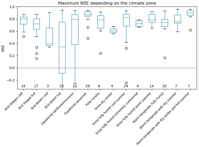
Figure 6 Box plot of the maximum NSE per climate zone. The green line indicates the median, the box extends from the 1st quartile (Q₁) to the 3rd quartile (Q₃), whereas whiskers go from $Q_{\mathrm{1}}-\mathrm{1.5}(Q_{\mathrm{3}}-Q_{\mathrm{1}})$ (or the minimum value if higher) to $Q_{\mathrm{3}}+\mathrm{1.5}(Q_{\mathrm{3}}-Q_{\mathrm{1}})$ (or the maximum value if lower). Circles denote basins lying outside of the whiskers. The numerals represent the number of basins in each climate zone.

Hot arid deserts also have a large spread in the water budget imbalance (Fig. 6). Among those basins, some were entirely desert (the Arabian Peninsula, the Sahara, Somalia, and South and West Australia) with a low signal-to-noise ratio, as previously mentioned. Other basins were partially covered by steppe (Australia, the Orange Basin, and around the Indus Basin) or equatorial savannah (Niger, Chad, and Nile basins). In those basins, precipitation occurred in the more humid subregions, thereby increasing TWS variations. As a consequence, the error in the datasets became less significant and allowed a proper budget reconstruction.

4.3 Overall combinations' performance

Although a majority of basins achieved a positive cyclostationary NSE, they differed greatly in terms of the number of combinations yielding positive values. As an example, 839 combinations satisfied a positive NSE_c in the São Francisco Basin whereas only 94 did so in the neighbouring Tocantins Basin (Fig. S9). Therefore, we wanted to evaluate the ability of a single combination to close the water budget worldwide. To do so, we evaluated the total area of basins with a positive cyclostationary NSE for each combination. Table 1 shows the 20 combinations leading to the largest area.

Table 1 Combinations with the largest area covered with a positive cyclostationary NSE.

Combinations are ranked by decreasing area of basins with a positive cyclostationary NSE. Italics indicate combinations where P, ET, and R are from the same model.

It appears that choosing all three variables (P, ET, and R) from ERA5-Land yields significantly better results than the other combinations (35.5 ×10⁶ km² with a positive NSE_c from the total study area of 96.6 ×10⁶ km²). Figure 7 indicates that ERA5-Land performed well in the central and eastern United States of America (USA), but it failed to provide the positive NSE_c of Fig. 4 in the mountainous western basins (Columbia, Great Basin). Again, in a comparison with the best possible results, ERA5-Land performed quite poorly in the equatorial region of South America (Amazon Basin and above), in Central Eurasia (around the Ob, Aral Sea, and Indus basins), and in several basins in Europe.

Knowing that at least one combination exists that gives a positive cyclostationary NSE in 62.3 ×10⁶ km², Table 1 shows that even the best combinations were far from approaching this number. This confirms that it is currently clearly impossible to achieve a good water budget closure with a single combination (Gao et al., 2010; Lorenz et al., 2014).

The second-best combination in terms of area satisfying a positive cyclostationary NSE was the CLSM forced with version 2.0 of GLDAS (in particular PGF precipitation). Table 1 shows that 30.8 ×10⁶ km² reached a positive NSE_c with this combination. Similar observations to those for ERA5-Land can be made generally, with good performance in central and eastern USA, southeastern America, and Australia. CLSM2.0 was more consistent than ERA5-Land in Europe but less so in Africa.

When looking at the following combinations, it appeared that their performance was more similar, compared with the differences observed between the two best combinations. Table 1 also shows that each variable has a determining impact on the water budget closure. Indeed, choosing, for example, CLSM2.2 for runoff instead of ERA5-Land (as shown in the left column of Fig. 7) led to poorer results in Alaska, Asia, and central Africa, whereas it improved NSE values around the Amazon Basin.

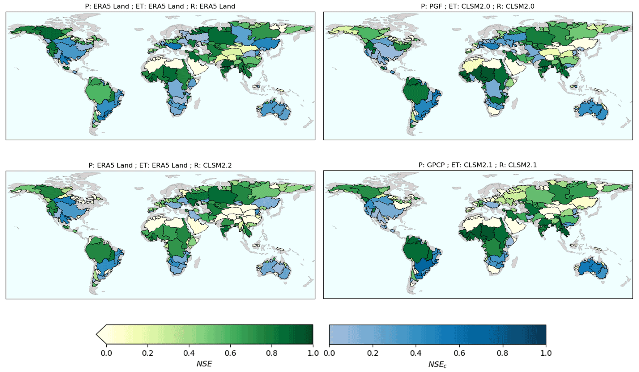
Figure 7 NSE and cyclostationary NSE with the first combinations in Table 1. Basins with a positive cyclostationary NSE are represented with blue shades corresponding to the NSE_c. The remaining basins are depicted in green, according to their NSE.

Concerning GLDAS LSMs, it is clear from Table 1 that CLSM was a globally better LSM than Noah and VIC. When using all variables from the same LSM, we also noted that GLDAS 2.0 was globally better than version 2.1 for all LSMs (CLSM, Noah, and VIC). As illustrated in the right column of Fig. 7, major differences are observed in Europe, western Russia, and Alaska. This can be explained by disagreement between precipitation from GPCP and PGF. For instance, CLSM2.1 yielded only low NSE values in most of eastern Europe, whereas version 2.0 of the same model achieved a positive cyclostationary NSE. This last finding reflects the conclusion of studies such as Mueller et al. (2011) and Zaitchik et al. (2010), who found that forcing variables have a considerable influence on land surface models' outputs.

We also point out that the ranking in Table 1 was not significantly modified by discriminating basins on the area satisfying a NSE larger than 0.5 (usually considered as good performance) instead of a positive cyclostationary NSE. This ensures the reliability of the method used to highlight the most consistent combinations.

4.4 Datasets suitable in given regions

In the previous section, numerous combinations of global datasets were evaluated. This section aims to describe regions where some datasets are more suitable than others to close the water budget. In a given basin, we defined suitable datasets as those appearing in combinations leading to a cost (difference between the maximum NSE and the NSE for a specific combination) lower than 0.1. This threshold was chosen to ensure that only the combinations with the best performance were considered as suitable. For this analysis, we focus on a subset of 132 basins, out of the 189, where an excellent budget closure could be achieved (maximum NSE larger than 0.8 or maximum NSE_c larger than 0.1).

In general, many combinations were below the maximum cost: at least 112 combinations were suitable in 50 % of the basins, and at least 185 combinations were suitable in 25 % of the basins. For a detailed review of suitable datasets in each basin, the reader is referred to Figs. S17–S20. Although there was a large choice of combinations to close the water budget, two basins with similar characteristics only had a few suitable combinations in common. This makes a global and comprehensive evaluation of datasets more complex.

In addition, we observed that suitable datasets in a basin could generally not be mixed, suggesting that some cancellation bias occurred. As an example, Fig. 8 shows that suitable datasets in the Mississippi Basin have considerably different seasonal cycles. Combining a precipitation dataset with high amplitude (GPCP) with low runoff (CLSM2.2) could close the water budget if associated with high evapotranspiration (CLSM2.1, leading to NSE_c=0.32) but not with low evapotranspiration (Noah2.0, ${\mathrm{NSE}}_{\mathrm{c}}=-\mathrm{1.8}$). As there is no reason to consider one dataset more reliable than others in the absence of unbiased observations, care must be taken when combining suitable datasets.

Figure 8 Datasets appearing in suitable combinations in the Mississippi Basin (cost lower than 0.1). The discrepancy is similar to the coefficient of variation, except that the numerator is the difference between the maximum and minimum values instead of the standard deviation.

In order to provide a general overview of datasets' performance, we choose to gather basins achieving the water budget closure for similar combinations. Those regions were determined with the hierarchical clustering described in Sect. 3.3. The 132 selected basins with a good water budget closure are depicted in the dendrogram in Fig. S10, and clusters represent basins with similar costs for the same combinations. We chose 13 such clusters comprising major basins of the world to provide a precise (but succinct as possible) overview of the datasets' performance. These clusters are denoted by the coloured lines in Fig. S10 and are shown with the same basin colours as on the map in Fig. 9.

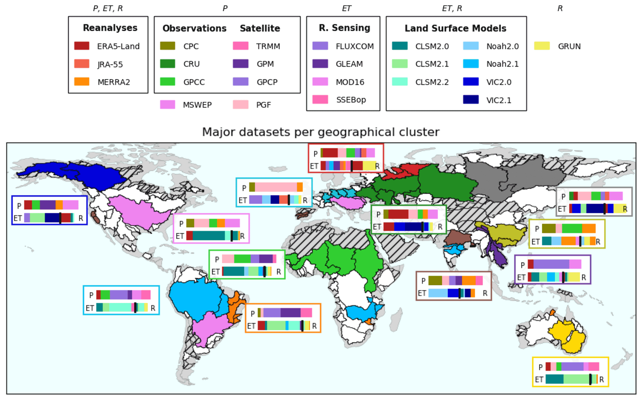
Figure 9 Datasets appearing in combinations that satisfy a cost lower than 0.1 for all basins inside the cluster. The 13 clusters highlighted in Fig. S10 are shown using different colours. For each cluster, the top line of each box represents precipitation datasets. The left part of the bottom line is evapotranspiration datasets whereas the right part is runoff. The limit between ET and R is symbolised by a black line located proportionally to the portion of ET in the mean annual water cycle of the corresponding region. Hatched areas show basins with a poor water budget closure (maximum NSE lower than 0.8 and maximum NSE_c lower than 0.1).

Basins clustered together in the dendrogram in Fig. S10 were either neighbouring basins (e.g. eastern Europe or eastern Australia) or basins with similar geographical conditions. Therefore, it is sensible that the same combinations performed well in those basins. Among basins with similar characteristics, we pointed out large rivers in temperate regions (Mississippi, Paraná, and Danube basins) or cold basins with different snow conditions (Yenisei, Lena, Mackenzie, Yukon, and Kolyma basins).

For each of the 13 clusters, we selected combinations yielding a cost lower than 0.1 in every basin of the region. Figure 9 shows which datasets can be used in combination to satisfy the water balance. Among the precipitation datasets, it first appears that the rain-gauge-based GPCC was often found in combinations satisfying the maximum cost, along with the satellite-augmented GPCP, reanalysis ERA5-Land, and the multi-source PGF. As a first approximation, those datasets are suitable for global water budget analyses. However, for regional analyses, a closer look at individual datasets is required to obtain all possibilities.

Figure 10 (top left) shows the decay in NSE when using GPCC as the precipitation dataset. It confirms that GPCC was very close to the best-performing precipitation datasets. Surprisingly, Fig. 10 also indicates that although GPCP added satellite measurements to GPCC observations, it increased the water budget imbalance in eastern Europe and western Russia as well as in Congo and South Africa. GPCP performed notably well in South America, along with ERA5-Land, which was one of the most consistent datasets for precipitation. The only region where ERA5-Land was not suitable was around China and Saint Lawrence Basin. As shown in Fig. 9, PGF precipitation was able to close the water budget predominantly in Europe as well as in Central Africa.

Figure 10 The mean of the 10th highest NSE with combinations comprising the reference dataset (i.e. GPCC, GPCP, PGF, or ERA5-Land) is compared to the mean of the 10th highest NSE excluding the reference dataset. Yellow indicates basins where the reference dataset is similar to or better than other precipitation datasets whereas blues show regions where it was significantly worse. Hatched areas show basins with a poor water budget closure (maximum NSE lower than 0.8 and maximum NSE_c lower than 0.1).

For comparison, Fig. S12 indicates that CRU, which never appears in the map Fig. 9, performed very poorly compared with other datasets. Harris et al. (2020) mentioned that no homogenisation of data was performed in CRU data. CRU also uses climatology values when measurements are missing, making it more appropriate for global analyses. The other rain-gauge-based dataset CPC was mainly suitable in Europe and China (see Fig. 9). As MERRA2 is based on CPC observations (except in Africa, where slight variations can be seen in Fig. S12), similar conclusions can be drawn for MERRA2. In addition, using GPM instead of TRMM (where we recall that GPM includes and extends TRMM results) improved the water budget closure. Finally, there was no overwhelming advantage in choosing the multi-source MSWEP dataset; it is consistent in Europe and South America but should be avoided in snow-dominated regions of eastern Russia and Alaska (Fig. S12).

Figure 9 clearly shows that evapotranspiration from the land surface model VIC should be chosen in Russian snow-dominated basins, with a preference for version 2.0 compared with 2.1. However, this dataset should not be used in hotter regions such as South America, Africa, or Australia (Fig. S11). We found that VIC produces less evapotranspiration than other datasets, along with higher runoff. CLSM was also consistently found in Fig. 9. Versions 2.0 and 2.1 performed similarly (except in Europe, where version 2.0 was better, as already mentioned) and were especially suitable in equatorial (South America, sub-Saharan Africa, and Australia) and some temperate regions (southeastern Europe and the USA). Similar to precipitation, ERA5-Land evapotranspiration is an excellent dataset in most of the regions except the Amazon Basin, China, and Australia (Fig. S11).

Evapotranspiration from CLSM version 2.2 provided a good water budget closure in most of South America, Europe, and especially South Asia. However, it led to unrealistic low values in snow-dominated basins (see Fig. S11). An example of this behaviour is given in Fig. S15 where highly negative values appear in autumn. As this dataset assimilates GRACE measurements and was validated against GRDC observations, this may reflect overfitting of runoff that is better constrained than evapotranspiration, leading to unrealistic ET values.

When examining specific evapotranspiration datasets (FLUXCOM, GLEAM, MOD16, and SSEBop), it appeared that GLEAM led to almost optimal NSE values in Africa and Europe (Fig. S14). We also compared the newly released version 3.5 of GLEAM with the older v3.3 used in this study and found that the new version slightly improved the budget closure in every basin (not shown). FLUXCOM was also consistent in North and South America, Europe, western Russia, and South Asia, although it was outperformed by CLSM and ERA5-Land. Finally, SSEBop and MOD16 brought little improvement to the water budget closure. The poor performance of MOD16 has already been highlighted by studies such as Pascolini-Campbell et al. (2020) in the CONUS and Bhattarai et al. (2019) in India.

The evaluation of runoff datasets in Fig. S13 confirms the differences exhibited for evapotranspiration (Fig. S11). VIC was mainly suitable in temperate and snowy regions, even if it performed quite poorly in some snow-dominated basins (Nelson, Saint Lawrence, and Pechora, among others) due to the overestimation of runoff during summer. It is also clear from Fig. S13 that this LSM is not well suited for equatorial and arid basins in South America (except some temperate basins in the extreme south), Africa, Australia, and part of Asia. In those basins, the machine learning model GRUN was exceptionally good, especially outperforming others in South America. In addition, except in the Amazon Basin and China, where it has already been said that ERA5-Land was not appropriate, this reanalysis yielded a good runoff estimation.

The low NSE decays in Fig. S13 indicate that CLSM version 2.2 provides accurate runoff estimations, which is the main objective of this dataset (Li et al., 2019). However, Fig. S13 shows that it did not improve the water budget closure achieved by version 2.0 of this same model. In some basins, like Congo, the water budget imbalance increased.

In a selection of 10 large basins with sufficient temporal coverage of GRDC gauge measurements (the Amazon, Congo, Mackenzie, Mississippi, Ob, Orange, Paraná, Volga, Yenisei, and Yukon basins), we additionally evaluated the maximum NSE (and cyclostationary NSE) that could be obtained using GRDC records as the only source of runoff data. We found that the water budget closure slightly improved in six basins and significantly improved in three basins. The only basin where a slight decrease could be observed was the Orange Basin. This suggests that users interested in using discharge measurements should not see the water budget closure worsening compared with the datasets we used, but care needs to be taken to ensure that the discharge data are of sufficient quality and completeness for the basin of interest.

5 Conclusions

We assessed the ability of various precipitation, evapotranspiration, and runoff datasets to close the water balance equation against satellite-observed terrestrial water storage anomalies on a global scale. Our analysis was comprehensive, as a large number of global datasets were used to prepare 1694 combinations for closing the water balance in the 189 catchments investigated. We found that the TWSC prediction was better than the long-term mean in 99 % of the study area and better than the monthly mean in 62 % of the study area. This illustrates that we can close the water balance equation in most of the regions if we choose certain datasets for budget components, which is a novel finding in terms of our previous understanding (Lorenz et al., 2014; Sahoo et al., 2011). We demarcated river catchments where the usual metrics (NSE, cyclostationary NSE) were of limited interest to evaluate the imbalance error.

Although the lowest imbalance error possible was generally small, we found that none of the 1694 combinations assessed succeeded in closing the water budget worldwide. Some combinations performed better in some regions but underperformed in others. The combination with all of the budget components from the ERA5-Land reanalysis was the best in terms of achieving a positive cyclostationary NSE over the largest fraction of the area under investigation. Individual components (P, ET, and R) of ERA5-Land were also close to the best-performing datasets, except for around the Amazon Basin and eastern China.

The Catchment Land Surface Model (CLSM) additionally appeared as a suitable dataset in many regions, excluding snow-dominated basins. However, version 2.2 of this LSM, which assimilates GRACE data, performed poorly compared with its previous versions. In some snow-dominated basins, it even led to highly unrealistic ET values during the cold season. Despite being designed for better runoff estimates, this latest version did not offer much improvement compared with other runoff datasets in terms of the water imbalance error. In contrast, GRUN, a machine learning runoff dataset, considerably reduced the imbalance error in several basins, with the best performance being detected in South America, South Asia, and some Arctic basins in Russia and Alaska.

We have presented a comprehensive overview of our ability to close the global water balance with the help of a wide range of water budget components disseminated for scientific studies. For each water budget component, we also assessed the performance of individual datasets with respect to the other datasets available, which helped us to infer the quality of the dataset when closing the water budget. We also found that the water balance can close due to a cancellation of errors in budget components; therefore, caution should be practised when closing the water budget over a catchment or region and a large number of datasets should be explored to avoid obtaining the right results for wrong reasons. We hope that our analysis will help fellow researchers in finding the most appropriate datasets for water budget analysis in different parts of the world.