Inundation prediction in tropical wetlands from JULES-CaMa-Flood global land surface simulations

Wetlands play a key role in hydrological and biogeochemical cycles and provide multiple ecosystem services to society. However, reliable data on the extent of global inundated areas and the magnitude of their contribution to local hydrological dynamics remain surprisingly uncertain. Global hydrological models and land surface models (LSMs) include only the most major inundation sources and mechanisms; therefore, quantifying the uncertainties in available data sources remains a challenge. We address these problems by taking a leading global data product on inundation extents (Global Inundation Extent from Multi-Satellites, GIEMS) and matching against predictions from a global hydrodynamic model (Catchment-based Macro-scale Floodplain – CaMa-Flood) driven by runoff data generated by a land surface model (Joint UK Land and Environment Simulator, JULES). The ability of the model to reproduce patterns and dynamics shown by the observational product is assessed in a number of case studies across the tropics, which show that it performs well in large wetland regions, with a good match between corresponding seasonal cycles. At a finer spatial scale, we found that water inputs (e.g. groundwater inflow to wetland) became underestimated in comparison to water outputs (e.g. infiltration and evaporation from wetland) in some wetlands (e.g. Sudd, Tonlé Sap), and the opposite occurred in others (e.g. Okavango) in our model predictions. We also found evidence for an underestimation of low levels of inundation in our satellite-based inundation data (approx. 10 % of total inundation may not be recorded). Additionally, some wetlands display a clear spatial displacement between observed and simulated inundation as a result of overestimation or underestimation of overbank flooding upstream. This study provides timely information on inherent biases in inundation prediction and observation that can contribute to our current ability to make critical predictions of inundation events at both regional and global levels.

1 Introduction

Wetlands and other inundated areas make up 6 %–8 % of the terrestrial ice-free land surface (Mitsch and Gosselink, 2000, 2015; Junk et al., 2013). However, this percentage greatly underestimates their importance to the global climate system (WMO, 2019) and to human society (Mitsch and Gosselink, 2000). Wetlands, including peatlands (bogs and fens), mineral soil wetlands (swamps and marshes), and seasonal or permanent floodplains play a key role in hydrological and biogeochemical cycles, are home to a large part of global biodiversity, and provide value to human society in the form of multiple ecosystem services (Junk et al., 2013). Most significantly, wetlands and other inundated areas

• i.

  provide a spectrum of ecosystem services to human society, including filtering of pollutants, maintenance of buffers against flood damage, reduction of soil erosion, biodiversity protection, and recreational opportunities (Mitsch and Gosselink, 2015; Junk et al., 2013; Maltby and Barker, 2009),

• ii.

  are the most significant natural source of atmospheric methane (CH₄), contributing 20 %–31 % of global emissions of this highly potent greenhouse gas (Saunois et al., 2020), and

• iii.

  mediate latent heat exchange between the atmosphere and the land surface, thereby greatly affecting the occurrence of deep convection and meso-scale precipitation systems (Taylor, 2010; Prigent et al., 2011; Taylor et al., 2018), with implications for the availability of freshwater resources (WMO, 2019).

1.1 Inundation extent

Inundation extent is a key impact variable related to wetland dynamics produced by hydrological models and is calculated from a sequence of water balance calculations carried out over the course of the water cycle (at canopy level, ground level, etc.) (Hewlett, 1982; Sutcliffe, 2004). Precipitation received at the land surface is divided at the top of any vegetation canopy (canopy interception, dividing into canopy storage, throughfall and canopy evaporation, e.g. Best et al., 2011) and then again at the ground surface (dividing into infiltration to soil water and groundwater, soil evaporation, surface ponding and runoff). Heavy or persistent precipitation events may cause surface water (pluvial) flooding (high levels of surface ponding), resulting in higher runoff into local water courses. Once contained in water channels, most water flows along the river network to the ocean (river routing), but high river flows may exceed channel capacity downstream, producing an areal extent of inundated water (overbank inundation). Land surface inundation, if it occurs, is greater or lesser as a result of a balance between all of these factors.

Globally, we consider wetlands defined in the widest sense of any permanently or temporarily inundated area outside permanent water bodies (Ramsar, 2016). Wetlands may be divided according to their hydrotopographical context (Wheeler and Shaw, 1995) into groundwater-maintained or groundwater-fed wetlands, where the effects of groundwater dominate over other processes (e.g. fens, the depressional wetlands of USEPA, 2002, the non-flooded wetlands of Miguez-Macho and Fan, 2012, or the groundwater-dependent wetlands of Froend et al., 2016), and fluvial inundation-maintained wetlands, where their existence depends primarily on their proximity to a water course that regularly overtops its banks (e.g. igapó and várzea forests of the Brazilian Amazon, Pires and Prance, 1985). Seasonally varying levels of inundation are primarily dependent on upstream precipitation and how this translates into these two forms of inflow and secondarily on the ambient rates of evaporation and infiltration (Marthews et al., 2019; Clark et al., 2015; d'Orgeval et al., 2008). Further classification of wetlands in terms of vegetation or substrate is not required for our study (but see Wheeler and Shaw, 1995, USEPA, 2002, Gerbeaux et al., 2018, and Ramsar, 2016). The characterization of the variation of inundation as a result of the cycles and variability of all these processes is the primary challenge in simulating and predicting inundation (Yamazaki et al., 2011).

1.2 Uncertainty in observations

Much of the uncertainty in the magnitude of important fluxes related to wetlands is attributable to the wide range of estimates of global inundated areas (Parker et al., 2020; Aires et al., 2018; Melton et al., 2013; Tootchi et al., 2019; Pham-Duc et al., 2017; Hu et al., 2017). The importance of reducing this uncertainty has long been known from the perspective of policymakers concerned with implementing natural flood management plans (Dadson et al., 2017; Moomaw et al., 2018; Junk et al., 2013) or working in regions where water resources are under threat (Mitsch and Gosselink, 2000; Vörösmarty et al., 2010). Over the last decade, this has additionally been recognized more widely in the scientific community in terms of predictions of climate change (Zhao et al., 2017; Thirel et al., 2015), but progress has been relatively slow because of the challenge of simultaneously improving both our observations and our predictions of global inundation extents.

Assessing the precise extent of natural wetlands and other inundated areas from remote sensing remains challenging across large regions (Dutra et al., 2015), especially in the context of constraining process models that produce estimates of wetland extent (see the discussion in Saunois et al., 2020). Observational uncertainty depends on the form of inundation (e.g. deep vs. shallow, colder vs. warmer water) and ambient conditions (e.g. flooding occurring during a storm under cloud cover vs. from snowmelt under clear conditions or occurring during night vs. day hours). Additionally, there are the more general uncertainties in remote sensing products stemming from thresholding assumptions and/or compositing (e.g. see Liang and Liu, 2020). Uncertainty in inundation extent observations continues to be an issue in any study based on remote sensing data; e.g. this uncertainty has recently been shown to be the most significant factor in global CH₄ budget uncertainty (Parker et al., 2020).

1.3 Uncertainty in model predictions

Many hydrologic models exist that are capable of simulating flood inundation; however, these models differ greatly in their sophistication, the breadth of water cycle processes included, and their optimal scale of application (Dutta et al., 2000; Beck et al., 2017a; Clark et al., 2015, 2017; Davison et al., 2016). Inundation models seldom include all forms of inundation and hydrological processes (Davison et al., 2016; Clark et al., 2015), and the absence of even one process can lead to significant underestimation of inundation extent (e.g. as found by Parker et al., 2018, for the process of overbank inundation). The storage and conveyance of water in lakes, floodplains, groundwater and river channels, especially, are generally simulated only with relatively high uncertainty in the current generation of land surface models (LSMs) (Marthews et al., 2019, 2020).

Most hydrological models are run uncoupled from the atmosphere and are therefore reliant on the availability of high-quality precipitation and other atmospheric driving data obtained from independent sources. Uncertainties in the precipitation-driving data may often be very significant and larger than the total uncertainty inherent within the model being run (Marthews et al., 2020). Previous studies have attempted to validate global hydrology models against global hydrology products (e.g. Beck et al., 2017a). However, many such studies evaluated only runoff or river flow against corresponding models (e.g. Zhao et al., 2017), without consideration of the areal extent of inundation as we have done in this study.

1.4 Model and study area selection

The Catchment-based Macro-scale Floodplain global flood simulation model (CaMa-Flood) was selected for our predictions of inundation extents because of its sophistication and the fact that it is already widely used (see Hoch and Trigg, 2019, Zhao et al., 2017, and references therein). CaMa-Flood is the only open-source global river routing model that is based on the local inertial approximation of the Saint-Venant equations (Bates et al., 2010; Dutta et al., 2000; Yamazaki et al., 2013; Fassoni-Andrade et al., 2018), which takes into account the backwater effects of downstream elements, i.e. the possible reversal of flow in particular reaches upstream from e.g. lakes, tributaries, and estuaries (Hidayat et al., 2011). By including these effects, CaMa-Flood is able to produce a much better characterization of many wetlands whose dynamics are dominated by surface water inundation.

CaMa-Flood requires runoff data for its simulations, which we obtained from runs of the UK Joint UK Land Environment Simulator (JULES) land surface model carried out previously through the EU eartH2Observe project (Schellekens et al., 2017; Sterk et al., 2020). We chose to use this JULES-based dataset because uncertainty in water cycle quantities for JULES was comparable to any other equivalent land surface model (Marthews et al., 2020) and because streamflow and runoff data produced by this model have already been validated at regional (Martínez-de la Torre et al., 2019) and global (Arduini et al., 2017) levels. Additionally, through using these models, our results can contribute to the current effort to include global flood inundation in the JULES model itself (Dadson et al., 2021; Lewis et al., 2018, 2019).

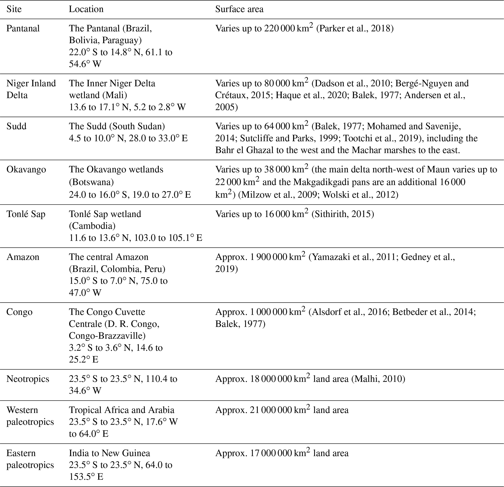
Our comparison of model and observational data is based on the observed Global Inundation Extent from Multi-Satellites Version 2.0 (GIEMS-2) dataset (Prigent et al., 2007, 2020). We analysed the tropical zone (23.5^∘ S to 23.5^∘ N, excluding small oceanic islands) at a resolution of 0.25^∘ in both latitude and longitude (Fig. 1). We have taken a case study approach (Table 1), where our wetland areas were selected on the basis of being the largest extant global wetlands, with two limitations. Firstly, we avoided regions with significant inundation on frozen and partially frozen land because GIEMS does not account for frozen water, and areas with significant snowfall are systematically masked as well (Prigent et al., 2007). Secondly, coastal or tidal wetlands were also avoided because their interactions with the ocean cannot currently be simulated by JULES or CaMa-Flood. Because of the preponderance of coastal occurrence across subtropical and temperate wetlands (Gumbricht et al., 2017; Melton et al., 2013), with these two limitations all remaining large wetlands were in the tropical zone (23.5^∘ S to 23.5^∘ N).

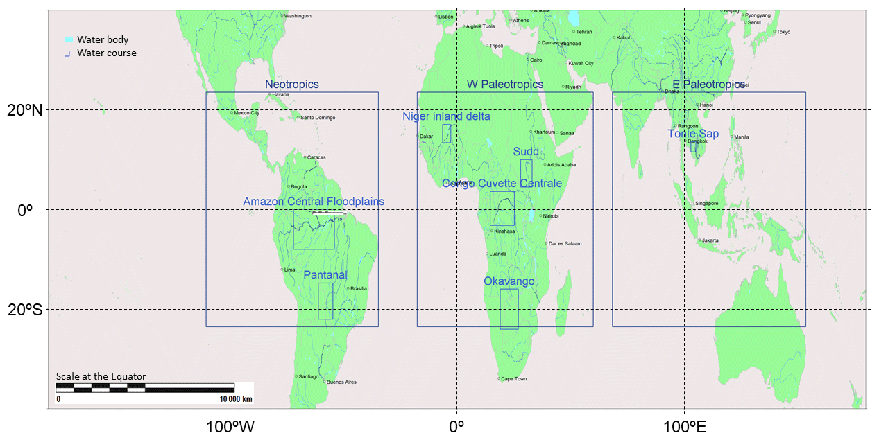
Figure 1 Tropical wetlands and inundated areas referred to in this study.

Table 1 The wetland case study areas. Total tropical land area is approx. 56 000 000 km² (approx. 38 % of total global land).

In this study, we ask the following questions.

1. How well can the CaMa-Flood model, driven by JULES runoff data at 0.25^∘ resolution, simulate observed global inundated extents, as given by GIEMS satellite-based data?

2. Can an improved match between observed and predicted inundation be obtained by simple transformations, e.g. removing low/high observed values or adding a constant to all predicted inundation fractions?

3. Are these simple transformations dependent on spatial scale (e.g. regional vs. subcontinental)?

Answering these questions will highlight both the strengths and weaknesses of the JULES-CaMa-Flood approach to global inundation prediction and indicate possible directions where improvements may be made in modelling predictive capability in global wetlands.

2 Methods

Observed and simulated inundation extents were compared at a global resolution of $\mathrm{0.25}{}^{\circ }\times \mathrm{0.25}{}^{\circ }$ (approximately 25 km × 25 km at the Equator).

2.1 Observed inundation extents

Observational data on monthly global inundation fraction were obtained from GIEMS-2 (Prigent et al., 2020), which is considered to be one of the best widely available global products of inundation extents and captures water under vegetation very well (Hu et al., 2017; Pham-Duc et al., 2017). Data were regridded to a regular spatial resolution of $\mathrm{0.25}{}^{\circ }\times \mathrm{0.25}{}^{\circ }$ to enable comparison to model outputs.

GIEMS is mainly derived from passive microwave observations (Special Sensor Microwave/Imager, SSM/I), with the help of active microwave and visible and near-infrared reflectance observations (Advanced Very High Resolution Radiometer, AVHRR) to eliminate ambiguities in surface water detection and to account for the potential contribution of vegetation (Prigent et al., 2007, 2020). GIEMS can detect inundation of both natural wetland and irrigated agricultural areas. Frozen surfaces are excluded. In unfrozen areas, the accuracy of GIEMS has been comprehensively verified (Papa et al., 2006, 2010), and it is a very widely used remote sensing product (Zhang et al., 2016; Taylor et al., 2018). Therefore, we suggest that it forms an appropriate benchmark dataset for global modelling studies.

2.2 Simulated inundation extents

Model-derived inundation extents were produced by a sequentially executed run of two models referred to here as JULES-CaMa-Flood.

2.2.1 Validation of land surface runoff

Predictions of land surface runoff were obtained from the JULES land surface model (https://jules.jchmr.org/, last access: 20 June 2022) (Best et al., 2011; Clark et al., 2011) by accessing simulations carried out previously through the EU eartH2Observe project (Schellekens et al., 2017; Sterk et al., 2020; Marthews et al., 2020). A description of the hydrological simulation approach and water balance calculations in JULES is given in Martínez-de la Torre et al. (2019) and Blyth et al. (2019). As discussed in Marthews et al. (2020), uncertainties in the precipitation driving data may often be significant, so we selected Multi-Source Weighted-Ensemble Precipitation (MSWEP), currently considered the best available global precipitation product at this spatial resolution (Beck et al., 2017b; Marthews et al., 2020). The model configuration used for JULES was global Water Resources Reanalysis Tier 2 (WRR2) (Fink and Martínez-de la Torre, 2017). Arduini et al. (2017) analysed runoff data from an ensemble of land surface models including JULES both at a global level and for the Amazon in particular, finding that JULES was not an outlier in relation to other models, performing well in terms of both annual cycle and year-on-year trends. Marthews et al. (2020) analysed the same eartH2Observe ensemble on a region-by-region basis, finding that the causes of higher model uncertainty operated differentially in wet and dry environments, with wetter environments being modelled with less uncertainty than dry environments. This supports our focus on global wetlands in this study and our use of JULES-derived runoff data.

2.2.2 Validation of land surface inundation

Daily runoff data from JULES were used to drive the CaMa-Flood v3.9.6a flood inundation model (version November 2019) (Yamazaki et al., 2009, 2011) to produce predictions of surface inundation at all points. CaMa-Flood was run with a timestep length of 1 min, and the outputs were averaged to produce monthly output data. CaMa-Flood was set to calculate river discharges and flow velocities using the local inertial equation along its river network map in order to include backwater effects (Bates et al., 2010; Yamazaki et al., 2011, 2013). In order to compare more easily to observations on a regular grid, our CaMa-Flood simulations were in fully grid-based mode rather than using irregularly shaped catchments (Yamazaki et al., 2009, 2011). CaMa-Flood's options for bifurcating flows within the model were not activated for these simulations (Yamazaki et al., 2014): we focus on water balance in our analysis (which should be negligibly affected by river braiding and other bifurcations).

3 Analysis

The period for which eartH2Observe and GIEMS-2 data overlap is 1992–2014, so we used this period for all our analyses. All post-processing steps were carried out using NetCDF Operator (NCO) tools v.4.4.5 (Zender, 2008) and the R v.4.0.2 statistical language environment (R Core Team, 2021). For the R-based analyses, packages maps, rgeos (v.0.5-3), GEOS runtime (v.3.8.0), and rgdal (v.1.5-12) were required.

3.1 Evaluation metrics

We applied the two most common efficiency statistics used in the context of river flow analysis: the Nash–Sutcliffe efficiency (NSE) and Kling–Gupta efficiency (KGE), both of which measure the alignment between model results and observations (Table 2). KGE is based on a decomposition of NSE into its constitutive components (correlation, variability bias, and mean bias) and addresses several perceived shortcomings in NSE (Knoben et al., 2019).

Table 2 Efficiency metrics widely used in flood model assessment and forecast verification (Knoben et al., 2019). In all the equations, Q is the flow variable (e.g. discharge) over time steps t=1, …, T. Subscripts “obs” and “sim” refer to observed and model-predicted values, respectively, ${\mathit{\mu }}_{\mathrm{obs}}=\stackrel{\mathrm{‾}}{Q_{\mathrm{obs}}}$ is the observation mean, ${\mathit{\sigma }}_{\mathrm{obs}}=\sqrt{\frac{\mathrm{1}}{N-\mathrm{1}}\sum _t{\left(Q_{\mathrm{obs}}\left(t\right)-\stackrel{\mathrm{‾}}{Q_{\mathrm{obs}}}\right)}^{\mathrm{2}}}$ is the standard deviation (and similarly for μ_sim and σ_sim), and r is the Pearson correlation coefficient between observed and simulated values.

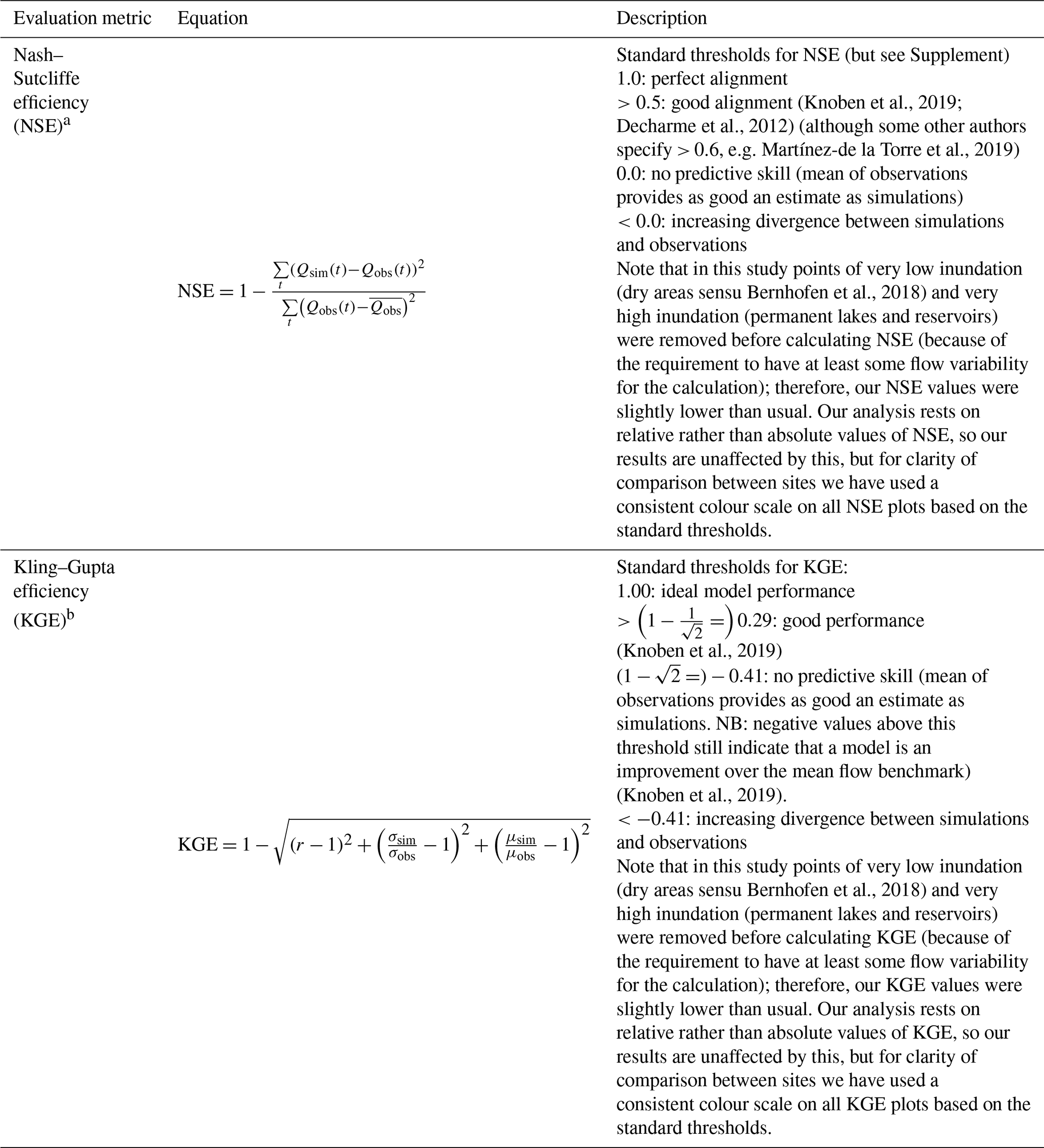
^a NB: both NSE and KGE are uncorrected for the magnitude of the variability of the observations σ_obs (see Supplement). ^b NB: KGE without the penalty terms (in μ and σ) reduces simply to Pearson's correlation coefficient (NB: the positive root is 1−r rather than r−1): $\frac{\mathrm{cov}\left(Q_{\mathrm{sim}}\left(t\right),Q_{\mathrm{obs}}\left(t\right)\right)}{{\mathit{\sigma }}_{\mathrm{sim}}{\mathit{\sigma }}_{\mathrm{obs}}}=\frac{\mathrm{1}}{N-\mathrm{1}}\frac{\sqrt{\sum _t\left(\left(Q_{\mathrm{sim}}\left(t\right)-\stackrel{\mathrm{‾}}{Q_{\mathrm{sim}}}\right)\left(Q_{\mathrm{obs}}\left(t\right)-\stackrel{\mathrm{‾}}{Q_{\mathrm{obs}}}\right)\right)}}{{\mathit{\sigma }}_{\mathrm{sim}}{\mathit{\sigma }}_{\mathrm{obs}}}$.

Our focus in this study is wetlands, and therefore we excluded areas of very high inundation (permanent lakes and reservoirs), which were always 100 % inundated in both observed and simulated data because of substitution from the Global Lakes and Wetlands Database, GLWD (Lehner and Döll, 2004), and also areas of continuously low or zero inundation (dry areas in the validation region, which would also provide a constant match between observed and simulated areas; see e.g. Bernhofen et al., 2018). Our focus on variability measures ensured that our match statistics were dominated by the regular (seasonal) and irregular cycles occurring at points where inundation was not constant, i.e. wetland regions sensu stricto.

3.2 Transforming inundation extents

When comparing the observed and simulated inundation extents, it can happen that inundation predicted by JULES-CaMa-Flood is not observed by GIEMS. Based on the data we have, it is not possible to be certain whether this “low-level” inundation shows some kind of bias towards overprediction on the part of the model or perhaps inundation actually occurred but was unobserved by GIEMS (see e.g. Liang and Liu, 2020, for a discussion on the limitations of the satellite-based sensors employed). In order to test this, during our analysis we posit a non-zero, minimum level of inundation fraction α_min, below which GIEMS always returns a zero result.

It is also possible that there is a maximum inundated fraction (here called α_max) above which GIEMS loses its sensitivity (i.e. possibly GIEMS can differentiate well between 20 % and 30 % inundation but not as reliably between 70 % and 80 %). This may possibly happen because vegetation canopy cover obscures inundation occurring beneath it, and the magnitude of this effect will depend on canopy coverage and the density of the canopy concerned, among other factors (GIEMS is capable of detecting some water under dense vegetation but with high uncertainty, especially when the distribution of inundation within the grid cell is highly skewed, i.e. small dry areas within a very wet grid cell or vice versa) (Prigent et al., 2020).

Finally, it may also be the case that our predictions of inundated fraction have a systematic bias (underestimation or overestimation, on a grid cell-by-grid cell basis). In order to test this, we introduce a fraction β which is added to all CaMa-Flood outputs of flooded fraction (fldfrc). In summary, we can modify the GIEMS data and CaMa-Flood outputs according to the simple transformations in Fig. 2 in order to investigate and quantify bias in both our simulated and observed data.

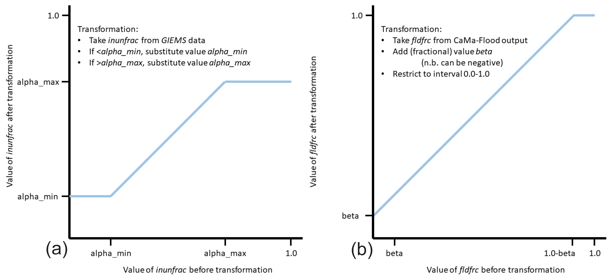
Figure 2 Transforming the GIEMS inundated fraction (inunfrac) data (a) and CaMa-Flood output flooded fraction (fldfrc) variable (b). Note that values ${\mathit{\alpha }}_{\min }=\mathit{\beta }=\mathrm{0.0}$ and α_max=1.0 are equivalent to making no modification.

4 Results

Results are presented in a sequence of case study areas, beginning with the Sudd, Pantanal, Tonlé Sap, Inner Niger Delta and Okavango wetlands before moving to the larger, subcontinental wetland complexes of the central Amazon and the Congo Cuvette. Straight comparisons between observations and model predictions of inundation show a complicated pattern of partial overlap that is challenging to assess visually (Fig. 3); therefore, we calculate appropriate statistics across all case study areas.

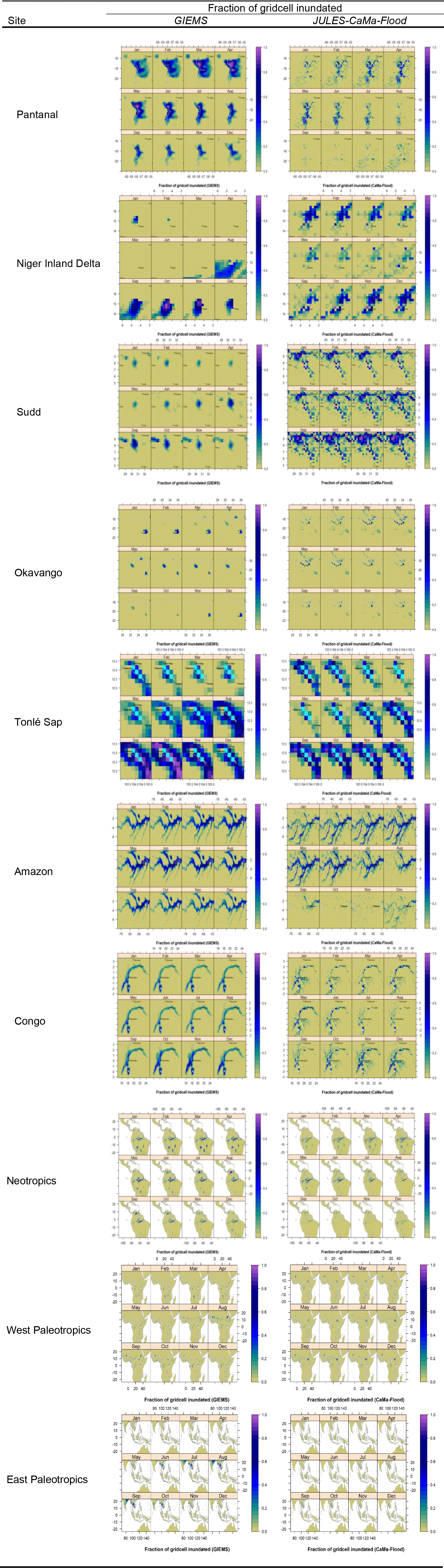
Figure 3 Fraction of grid cells inundated (in addition to water contained in channels and watercourses, which are not shown) in each study area. Superposed lakes and reservoirs are from the Global Lakes and Wetlands Database, GLWD (Lehner and Döll, 2004). Resolution is 0.25^∘ in both latitude and longitude (NB: Tonlé Sap is our smallest wetland, and therefore the grid cells are relatively large in that plot). View window extent is taken from references in Table 1. Cities with populations > 100 000 are shown (SimpleMaps, 2019) for view extents up to 2 000 000 km². Data shown are an average for 1992–2014 from GIEMS-2 observations (left-hand-side panels) and equivalent JULES-CaMa-Flood simulations (right-hand-side panels).

4.1 Inundation extent

GIEMS observations and JULES-CaMa-Flood predictions match very variably: monthly average inundation extent shows a clear bias in most study wetlands, and in addition there is significant year-on-year variability (Fig. 4). However, the direction of bias is not consistent between wetlands. NSE and KGE scores were calculated for each wetland study area in order to be able to compare consistently the match between simulated and observed wetland and inundation extents. NSE and KGE are metrics based on calculations of error (normalized root-mean-squared error, nRMSE) and correlation (Pearson's r correlation coefficient) (Table 2). We do not report calculated values of nRMSE or Pearson's r because plots of these statistics contained no information not visible on the corresponding plots of NSE and KGE.

Figure 4 Seasonal variation in inundation across the study wetlands, averaged across the years 1992–2014: red: observations (GIEMS); blue: simulated (JULES-CaMa-Flood). The three main tropical zones are not shown because they include areas both north and south of the Equator.

Because of our grid-cell-based approach, we could apply our NSE and KGE calculations in a distributed way across each case study wetland. These scores are most usually used in relation to discharge data, yielding generally only one time series per catchment (see Supplement), but our inundation estimates at every grid cell enabled us to calculate efficiency on a grid cell-by-grid cell basis in each of our study areas (Fig. 5). Averaged efficiency scores are generally high across each individual wetland although lower in parts of the wetlands that have the most dynamic flow regime.

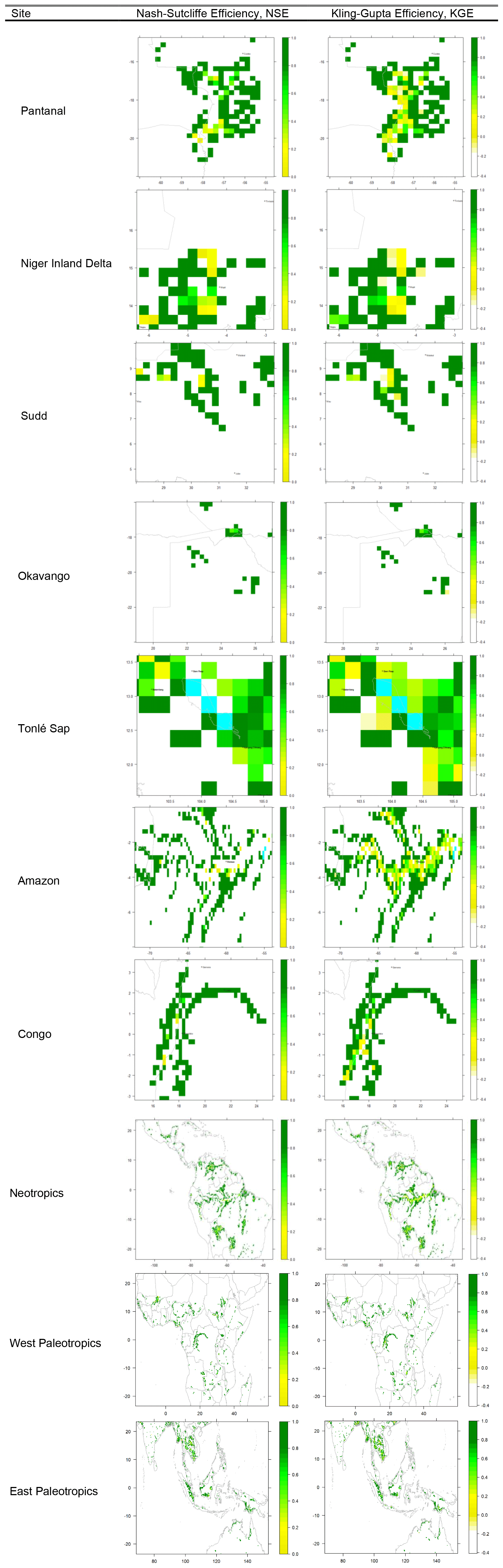
Figure 5 Mapped values for efficiency statistics based on inundated grid-cell fraction, averaged across the years 1992–2014 (with α_min=0.0, β=0.0 and α_max=1.0) (white indicates no value could be calculated).

However, NSE and KGE are not capable of measuring some important aspects of the flow regime, most notably spatial displacement of inundation, which might indicate that inundation input is overestimated in one area by the model at the expense of underestimation elsewhere, or, alternatively, might indicate that inundation inputs have been correctly calculated at all points, but an underestimated flow speed produces inundation at an incorrect location. For example, the Inner Niger Delta wetland shows apparent spatial displacement between observed and simulated inundation: GIEMS reports negligible inundation north of 15.5^∘ N in any month (a result broadly in line with the finer-scale analysis of Bergé-Nguyen and Crétaux, 2015), even though CaMa-Flood predicts inundation reaching as far as Timbuktu at 16.5^∘ N (Fig. 3). At this spatial resolution, 1^∘ latitude is well resolved, so this is a significant mismatch.

4.2 Identifying an optimal transformation of GIEMS observations and JULES-CaMa-Flood predictions

Varying the values of the three parameters α_min, α_max and β (see Fig. 2), we searched for an optimal value of each that brought our observed and simulated data as close together as possible, in order to quantify and therefore help understand the discrepancy between our model result and the (uncertain) observations. By repeating the calculations that produced Fig. 5 for an exhaustive range of parameter combinations of α_min, α_max and β, the state space plots in Fig. 6 were produced. A notably higher value for NSE or KGE for a particular combination of α_min, β and α_max identifies a consistent bias in either the model predictions or the observations (or both).

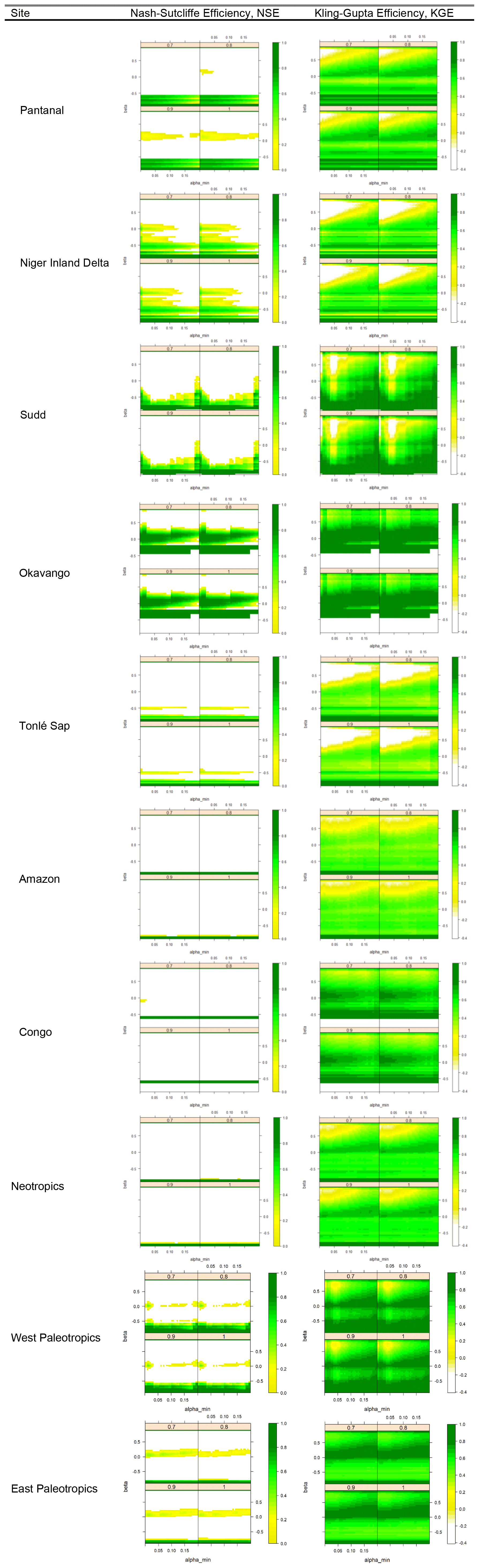
Figure 6 State space plots for evaluation statistics based on inundated grid-cell fraction, calculated from varying parameters α_min and beta, with panels showing values of α_max. Each point is the mean of all NSE or KGE values, averaged both over time (years 1992–2014) and over the wetland region concerned (white indicates no value could be calculated).

The visible maxima on our state space plots provide a best estimate of the optimal values of these parameters, with these optima differing markedly between our wetland study areas (Fig. 7). We found that α_min took a non-zero value ∼10 % across most of our study wetlands (Fig. 7) but found no evidence to suggest that α_max should consistently take any value < 1.0 for any of our wetlands (Fig. 6; i.e. we found no evidence that the GIEMS-2 inundation extents overestimated inundated fraction in grid cells where inundation covered a large percentage of the spatial cell).

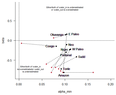
Figure 7 Summary of plots in Fig. 6. Optimal values of β and α_min are shown (referred to as β_opt and α_min opt in the text), calculated as the centroids of the maximal region on the KGE plots (black) or NSE plots (red) for each site (with α_max=1.0) from Fig. 6. On this plot, we define water_in = (channel + surface + subsurface inflow + precipitation) and water_out = (infiltration + evaporation). Note that clear maxima were not present for all case studies for NSE (Fig. 6), but when present they are shown connected to the equivalent maxima for KGE.

We found high variation in the estimated value of β for each wetland; i.e. adding a consistent constant fraction of inundation extent to all grid cells within the limits of each study wetland did indeed provide a closer match between observations and simulation, at least in the wetlands we considered in this study (Fig. 7). Defining water_in = (channel + surface + subsurface inflow + precipitation) and water_out = (infiltration + evaporation), we suggest that the negative values of β_opt in the Amazon, Tonlé Sap, Sudd and Inner Niger Delta show probable underestimation of hydrological output by JULES-CaMa-Flood (water_out) (Fig. 7). Conversely, the positive values of β_opt in the Okavango show probable underestimation of hydrological input by JULES-CaMa-Flood (water_in) (Fig. 7).

Finally, we note the specificity of our results to the time period 1992–2014. Carrying out this analysis for an earlier or a later period would most likely have yielded different estimates of NSE, KGE, α_min, α_max and β. However, we suggest that, without significant climate change or perhaps significant anthropogenic modification of the wetland area concerned, the values of these statistics should remain similar to the values calculated here.

5 Discussion

There has recently been significant progress in our understanding of wetlands and the roles they play in climate processes, land surface processes and their impacts on human society (Saunois et al., 2020; IPCC, 2014; Mitsch and Gosselink, 2015; Moomaw et al., 2018). However, even though the physics of flood inundation is relatively well known (Yamazaki et al., 2013; Bates et al., 2010; Fassoni-Andrade et al., 2018), many hydrological processes relevant to the representation of flooding in Earth system models remain poorly characterized at the high resolutions required to address issues of local and regional impact (Marthews et al., 2019; Zhou et al., 2021a; Bierkens, 2015; Clark et al., 2015), including infiltration (d'Orgeval et al., 2008; Clark et al., 2015) and evaporation (Robinson et al., 2017; d'Orgeval et al., 2008) of flood waters as well as groundwater effects (Clark et al., 2015).

In this study, we have simulated inundation extent at a spatial resolution high enough to resolve the major details of most major global wetlands. These results are potentially of great use to a wide audience of academic and non-academic users interested in the broad-scale impacts of environmental change in wetlands, especially where seasonal inundation affects water and energy fluxes in Earth system models. It is therefore appropriate to seek as robust a validation of these predictions as possible.

5.1 Comparing simulated and observed global inundated extents

We found that our simulated inundation extents (from the CaMa-Flood model, driven by JULES runoff data at 0.25^∘ resolution) sometimes compared very closely to our observed data (from GIEMS satellite-based data), but at many points there were divergences. For example, in the Sudd wetland, our model appears to overpredict inundation, whereas in the Pantanal wetland it appears to underpredict inundation. Can we explain these and other differences between GIEMS observations and our model predictions?

CaMa-Flood flood extent and GIEMS wetland extents do capture slightly different water surfaces. CaMa-Flood is most accurate in representing river-originated, fluvial flooding, and water surfaces not well connected to rivers have higher uncertainty (e.g. water bodies in local depressions due to rain-fed pluvial flooding). Additionally, GIEMS may overestimate the surface water extent in very wet areas (e.g. soils close to saturation but without a standing water surface).

In order to investigate these divergences, we applied simple transformations to our data, and the optimal values of the three parameters α_min, α_max and β we found for each wetland provide robust explanations for observable differences. We found that our predictions of inundation extent could be improved at local or regional scale by simple transformations involving the three parameters α_min, α_max and β. Moreover, in what follows we use our diagnosis of these differences to highlight opportunities to improve the representation of physical processes in land surface and large-scale hydrodynamic models.

We found evidence that α_min might generally take a non-zero value ∼10 % across tropical inundated areas, indicating that GIEMS-2 may be underestimating widely distributed occurrences of low inundation within these wetlands, as suggested by previous studies (Prigent et al., 2007). GIEMS may underestimate low levels of inundation that occur outside wetlands because of uncertainties in estimating inundation, e.g. below intact forest canopies (although small in any particular location, these would sum to a significant missing term in regional and continental water budgets).

We found high variation in the estimated value of β for each wetland, i.e. the constant fraction of inundation extent that must be added to all grid cells within the limits of each study wetland to elicit the closest match between observations and simulation. Defining water_in = (channel + surface + subsurface inflow + precipitation) and water_out = (infiltration + evaporation), we found in this study that some wetlands show underestimation of hydrological output by JULES-CaMa-Flood (water_out) (e.g. Amazon, Tonlé Sap, Sudd and Niger Inland Delta), whereas some show underestimation of hydrological input by JULES-CaMa-Flood (water_in) (e.g. Okavango). From a basic comparison of observed and modelled inundation extent, it is not possible to identify the precise combination of climate, season or hydrotopography that produces these underestimations and overestimations of water balance in these particular wetlands, but identifying the sign of the imbalance is nevertheless very useful information for interpreting model predictions in these areas.

The spatial displacement of inundation prediction downstream from observed inundation visible especially in our results for the Inner Niger Delta and the Sudd is a result of overestimation or underestimation of overbank flooding upstream. If overbank flooding is underestimated in our simulation, then the water within the river course (the Niger or White Nile, respectively, in these cases) will remain in the river and be taken downstream further than expected, producing a downstream wetland “extension” that exists in the simulation results but not the observed results (as we see in our JULES-CaMa-Flood outputs).

5.2 Quantifying bias in JULES-CaMa-Flood inundation predictions

Uncertainty in our model-derived inundation extents such as those from JULES-CaMa-Flood simulations is a combination of uncertainty from various sources, most immediately, the calculations within CaMa-Flood to predict inundation extent from runoff but also the runoff calculations within JULES and, before that, the precipitation data as well. When comparing to observational data, a fourth source of uncertainty is bias in observations, i.e. GIEMS-2 in this study.

The JULES-CaMa-Flood modelling sequence used in this study is an example of “uncoupled routing” where one model produces the runoff and a second model running separately calculates inundation, rather than both steps being integrated into a single model. This has significant advantages in terms of simplicity and ease of use in comparison to coupled alternatives but also disadvantages, especially in the context of wetland simulation. For example, in a mixed wetland such as the Pantanal with water input derived from both groundwater effects (lateral inflow – in the absence of any visible stream – from surrounding areas where the water table is higher than the wetland surface) and fluvial effects (overbank inundation from a stream or river), the groundwater input will be calculated by the runoff-generation routine (e.g. JULES), but the fluvial component will be calculated by the routing/flooding routine (e.g. CaMa-Flood). Separate simulation of these two input processes is undesirable, for example because CaMa-Flood does not calculate runoff and it includes no representation of a soil column and therefore does not have any explicit representation of subsurface processes, which means that important processes such as infiltration, which controls how wetlands recede in dry spells, can only be represented very approximately.

Do our optimal values for α_min, α_max and β indicate model simulation bias in JULES-CaMa-Flood under certain conditions? Perhaps yes: for example, the optimal parameter value β_opt may be understood as an estimate of the amount that is missing in the overall wetland water balance. For example, β_opt will be negative if evaporation and infiltration are being significantly underestimated by JULES-CaMa-Flood in this study area (neither JULES nor CaMa-Flood explicitly models evaporation from inundated water in their present configurations). Conversely, β_opt will be positive if e.g. groundwater inflow is being underestimated. More precisely, the value of β_opt may be thought of as an estimate of how much water_in is underestimated by JULES-CaMa-Flood minus how much water_out is underestimated. This estimate indicates model bias and also provides a measure of the direction and magnitude of that bias.

5.3 Implications for the hydrodynamic balance of wetlands

Wetlands exist as a balance between water input and water output, (i.e. water_in and water_out above, a landscape-scale water balance sensu Sutcliffe, 2004). In order to understand these and other points of divergence between observation and prediction, we need to understand this balance calculation in that particular wetland and also assess which types of water bodies are represented in the simulated data (Zhou et al., 2021a, b).

Categorizing wetlands in terms of positive or negative β_opt would be superficially similar to the division by Junk et al. (2011) of South American wetlands into fluvial (wetlands that are predominantly maintained by river overbank inundation rather than by groundwater effects) and interfluvial wetlands (where groundwater effects dominate); however, theirs was a distinction based on overall water balance rather than the balance of water input. In the context of our analysis here, we understand fluvial and interfluvial wetlands to mean ones where water_in is dominated by channel/surface flow or subsurface inflow, respectively. Both fluvial and interfluvial wetlands may of course experience high evaporation rates (e.g. the Inner Niger Delta) or high infiltration rates (based on underlying soil type) and therefore may occur either above or below the y=0 line in Fig. 7.

5.4 Inundation at subcontinental and larger scales

Looking at subcontinental scales (the Amazon and the Congo) and larger scales (the three main tropical zones), a number of additional considerations become more important. As with all very large river basins, the inland reaches of the Amazon and the Congo are collectively enormous wetland complexes, with some areas dominated by river flow and others by topographic factors (e.g. the “cuvette” of the Congo Cuvette indicates that the whole subcontinent is approximately a shallow bowl). The same diagnosis of biases may be carried out over these larger areas, but our optimal value for β generally converges closer and closer to the “null” value β=0.0 as larger and larger regions are considered (at least for regions that do not include significant coastal or permafrost areas). This is reasonable, because even the largest wetland areas are localized regions at this scale, and therefore these optima will be averaged together with an increasing number of relatively terra firme grid cells (i.e. grid cells which experience little or no regular inundation) and, at the largest scales, with entire mountain ranges where little or no inundation occurs (either in our model or in the observations).

In addition, we should expect that β_opt should converge to zero at the largest scales because we know that these models return reliable global estimates (Yamazaki et al., 2011); therefore, from a global perspective, the magnitude of values for a particular wetland or wetland complex should be understood as biases that are balanced out elsewhere. However, wetland-specific values nevertheless provide useful information about the inundation processes that dominate in those particular wetlands and allow us to improve our understanding of landscape-scale and continental-scale inundation hydrodynamics.

5.5 Conclusions

Simulations of inundation extent are important because they allow us to predict what will happen to globally important wetlands in the future. Wetlands are known to be key nodes in the biosphere system in terms of vulnerability to climate change (Maltby and Barker, 2009; Mitsch and Gosselink, 2015). However, wetlands are also highly dynamic landscape-level entities produced by the balance of a number of different water cycle processes acting together (Hewlett, 1982; Sutcliffe, 2004), not all of which are as yet represented in global hydrodynamic models (Yamazaki et al., 2011, 2013).

Reducing uncertainty in predictions from large-scale inundation models has long been a prerequisite for their use in global Earth system models. In this study we have shown that a very reasonable and close match may be derived between JULES-CaMa-Flood model predictions of inundation extent and independent GIEMS-2 global satellite-based observations of inundation. Differences do occur at regional scale, in particular large wetlands, however, and these differences indicate clearly the importance of incorporating into the modelling framework a better representation of the hydrological impacts of, especially, infiltration, evaporation and groundwater-fed inundation. These comments are not only relevant to GIEMS-2 and JULES-CaMa-Flood data: all satellite-based inundation data have biases that may be assumed to be very similar to those inherent in GIEMS data, and all model predictions of inundation have biases and uncertainties presumably similar to those that are in JULES-CaMa-Flood predictions (Dutra et al., 2015; Liang and Liu, 2020; Parker et al., 2020; Saunois et al., 2020), so we believe that our results and analysis provide a blueprint for users of other model/observational data on how they might assess and account for these types of bias in their own data.

Improving our understanding of the dynamics of inundated areas and the role they play in the generation of land–atmosphere fluxes requires a better representation in general of wetlands within global land surface and hydrodynamic models (Zhang et al., 2016). The results of this study point clearly towards the need for greater attention to be paid to hydrological dynamics and water cycle processes within these models, which we expect to result in improved modelling predictive capability in global wetlands in the future. A firm focus on producing a better characterization of hydrodynamics within this class of models will produce enormous positive returns in terms of our global capability to predict inundation and its global impacts and will make a welcome contribution to our preparedness for the impacts of future climate change (Moomaw et al., 2018; IPCC, 2014).