the Creative Commons Attribution 4.0 License.
the Creative Commons Attribution 4.0 License.
 | 17 Jun 2022
Agricultural intensification vs. climate change: what drives long-term changes in sediment load?
Shengping Wang
Borbala Szeles
Carmen Krammer
Elmar Schmaltz
Kepeng Song
Yifan Li
Zhiqiang Zhang
Günter Blöschl
Peter Strauss
Climate change and agricultural intensification are expected to increase soil erosion and sediment production from arable land in many regions. However, to date, most studies have been based on short-term monitoring and/or modeling, making it difficult to assess their reliability in terms of estimating long-term changes. We present the results of a unique data set consisting of measurements of sediment loads from a 60 ha catchment – the Hydrological Open Air Laboratory (HOAL) – in Petzenkirchen, Austria, which was observed periodically over a time period spanning 72 years. Specifically, we compare Period I (1946–1954) and Period II (2002–2017) by fitting sediment rating curves (SRCs) for the growth and dormant seasons for each of the periods. The results suggest a significant increase in sediment loads from Period I to Period II, with an average of 5.8 ± 3.8 to 60.0 ± 140.0 t yr−1. The sediment flux changed mainly due to a shift in the SRCs, given that the mean daily discharge significantly decreased from 5.0 ± 14.5 L s−1 for Period I to 3.8 ± 6.6 L s−1 for Period II. The slopes of the SRCs for the growing season and the dormant season of Period I were 0.3 and 0.8, respectively, whereas they were 1.6 and 1.7 for Period II, respectively. Climate change, considered in terms of rainfall erosivity, was not responsible for this shift, because erosivity decreased by 30.4 % from the dormant season of Period I to that of Period II, and no significant difference was found between the growing seasons of periods I and II. However, the change in sediment flux can be explained by land use and land cover change (LUCC) and the change in land structure (i.e., the organization of land parcels). Under low- and median-streamflow conditions, the land structure in Period II (i.e., the parcel effect) had no apparent influence on sediment yield. With increasing streamflow, it became more important in controlling sediment yield, as a result of an enhanced sediment connectivity in the landscape, leading to a dominant role under high-flow conditions. The increase in crops that make the landscape prone to erosion and the change in land uses between periods I and II led to an increase in sediment flux, although its relevance was surpassed by the effect of parcel structure change under high-flow conditions. We conclude that LUCC and land structure change should be accounted for when assessing sediment flux changes. Especially under high-flow conditions, land structure change substantially altered sediment fluxes, which is most relevant for long-term sediment loads and land degradation. Therefore, increased attention to improving land structure is needed in climate adaptation and agricultural catchment management.
- Article
(5498 KB) - Full-text XML
- BibTeX
- EndNote


Soil erosion is a phenomenon of worldwide importance because of its environmental and economic consequences (García-Ruiz, 2010; Prosdocimi et al., 2016). Climate change, land use and land cover change (LUCC), and other anthropogenic activities are commonly considered potential agents that drive variation in soil erosion rates (Nearing et al., 2004; X. A. Zhang et al., 2021). The impacts of climate change (e.g., Nearing et al., 2004; Zhang and Nearing, 2005; Mullan, 2013; Palazon and Navas, 2016) and of LUCC (e.g., Bochet et al., 2006; Korkanç et al., 2018; Nampak et al., 2018; S. Li et al., 2019; Perović et al., 2018) on erosion have been studied in recent years. As the two agents usually exert their influence on soil erosion simultaneously, their relative contributions have also been increasingly investigated (e.g., Bellin et al., 2013; Sun et al., 2020; X. A. Zhang et al., 2021). Combining field investigations with model simulations, X. A. Zhang et al. (2021) quantitatively evaluated the contributions of the decrease in annual rainfall erosivity, the decrease in arable land and bare land, and the construction of silt trap dams to the reduction of the sediment load of a typical watershed in the Loess Plateau area between 1987 and 2016, with the contribution values being +29 %, +40 %, and +31 %, respectively. Scholz et al. (2008) modeled how management practices at the local scale would affect soil erosion compared with climate change. They concluded that conservational management practices would have a greater impact on reducing soil erosion rates than the forecasted effects of climate change (i.e., the decrease in rainfall amounts in erosion-sensitive months). Moreover, soil erosion accelerated by livestock grazing was found to be more important than climate change on the Qinghai–Tibet Plateau (Y. Li et al., 2019).
Previous studies have provided valuable information on understanding how LUCC and climate change affect soil erosion and sediment load. However, it seems that most of the previous studies have considered LUCC (a change in land use and/or types of crops) and landscape structure change (a change in parcel size and structure) together. The relevance of landscape structure changes alone has currently received less attention. However, land use policies, such as land consolidation, have changed agricultural practices to a large extent since 1945, the beginning of agricultural industrialization (e.g., Moravcová et al., 2017; Devátý, et al., 2019), and, in particular, in countries where this process is relatively recent (Bouma et al., 1998; Moravcová et al., 2017; Y. Zhang et al., 2021).
Landscape structures usually influence erosion due to the boundary effects between land uses and land units (parcels) that differ with respect to water and sediment-trapping capacity (Baudry and Merriam, 1988; Merriam, 1990; Takken et al., 1999; Phillips et al., 2011). Van Oost et al. (2000) and Devátý, et al. (2019) evaluated the role of landscape structure by accounting for its spatial connectivity using modeling approaches and found that landscape structure is an essential factor when assessing the risk of soil erosion affected by land use changes. Both studies emphasized the potential impacts of land parcel structure changes on sediment production through altering hydrological and sediment connectivity. However, both studies relied on models and made assumptions regarding connectivity. Instead of focusing on the spatial connectivity, others (e.g., Bakker et al., 2008; Sharma et al., 2011; Chevigny et al., 2014; Wang et al., 2021; Tang et al., 2021; Madarász et al., 2021) evaluated the effect of terrain, soil properties, lithology, management practices, and other processes associated with landscape and/or land structure changes, and they highlighted their impact on sediment production. It has also been shown that the impact of landscape structure on erosion is more heterogeneous when different crops are grown, and the underlying lithology, soil properties, and topography show substantial spatial variability across the catchment (David et al., 2014; Cantreul et al., 2020).
In our analysis, we evaluate the relative roles of climate change, LUCC, and the change in land structure on sediment production. We define LUCC as a change in either the type of land use (e.g., arable land, grassland, forest) or the type of land cover (i.e., agricultural management, mainly by crops with different risk of soil erosion). We focus on understanding the respective role of LUCC and landscape structure change, based on long-term observations that have generally not been available in previous studies. We present the results of a unique data set consisting of measurements of sediment loads from a small agricultural catchment over a time window of 72 years. The study catchment is the 66 ha Hydrological Open Air Laboratory (HOAL) located in Petzenkirchen, Austria (Blöschl et al., 2016); this catchment, in addition to being exposed to climate change, has experienced a significant change in land use and land cover as well as parcel structure due to changes in land management policies during the past decades. Both discharge and suspended sediment concentration have been monitored periodically in the HOAL catchment from 1945 to 1954 and from 2000 to present. This provides an opportunity to disentangle the impacts of land structure change, LUCC, and climate change based on long-term measurements. Specifically, we aim at (i) exploring how the sediment regime shifted between the periods of 1945–1954 and 2002–2017, (ii) analyzing whether climate change or LUCC (or both) were responsible for any change in the sediment regime, and (iii) identifying the relevance of land structure change (i.e., land consolidation) on erosion control compared with LUCC.
2.1 Catchment characteristics
The HOAL catchment is situated in Lower Austria's alpine forelands (48∘9′ N, 15∘9′ E) with elevations ranging from 268 to 323 m a.s.l. and a size of 66 ha (Fig. 1). The climate of the catchment belongs to the temperate, continental climate zone (Dfb) according to the Köppen–Geiger classification (Kottek et al., 2006). The mean annual precipitation is 746 mm (1946–2006), with 62 % of the rain falling between May and October. The mean daily air temperature is 8.8 ∘C (1946–2006). The dominant land use is arable land, accounting for 82 % of the catchment land use on average over the past few years. Typical crops include winter wheat, corn, and barley. Deciduous trees grow along the stream (6 %), 10 % of the area is grassland, and 2 % is paved. The subsurface of the catchment consists of Tertiary marine sediments. Soils are classified into five types: calcic Cambisol, vertic Cambisol, gleyic Cambisol, Planosol, and Gleysol (IUSS Working Group WRB, 2015).
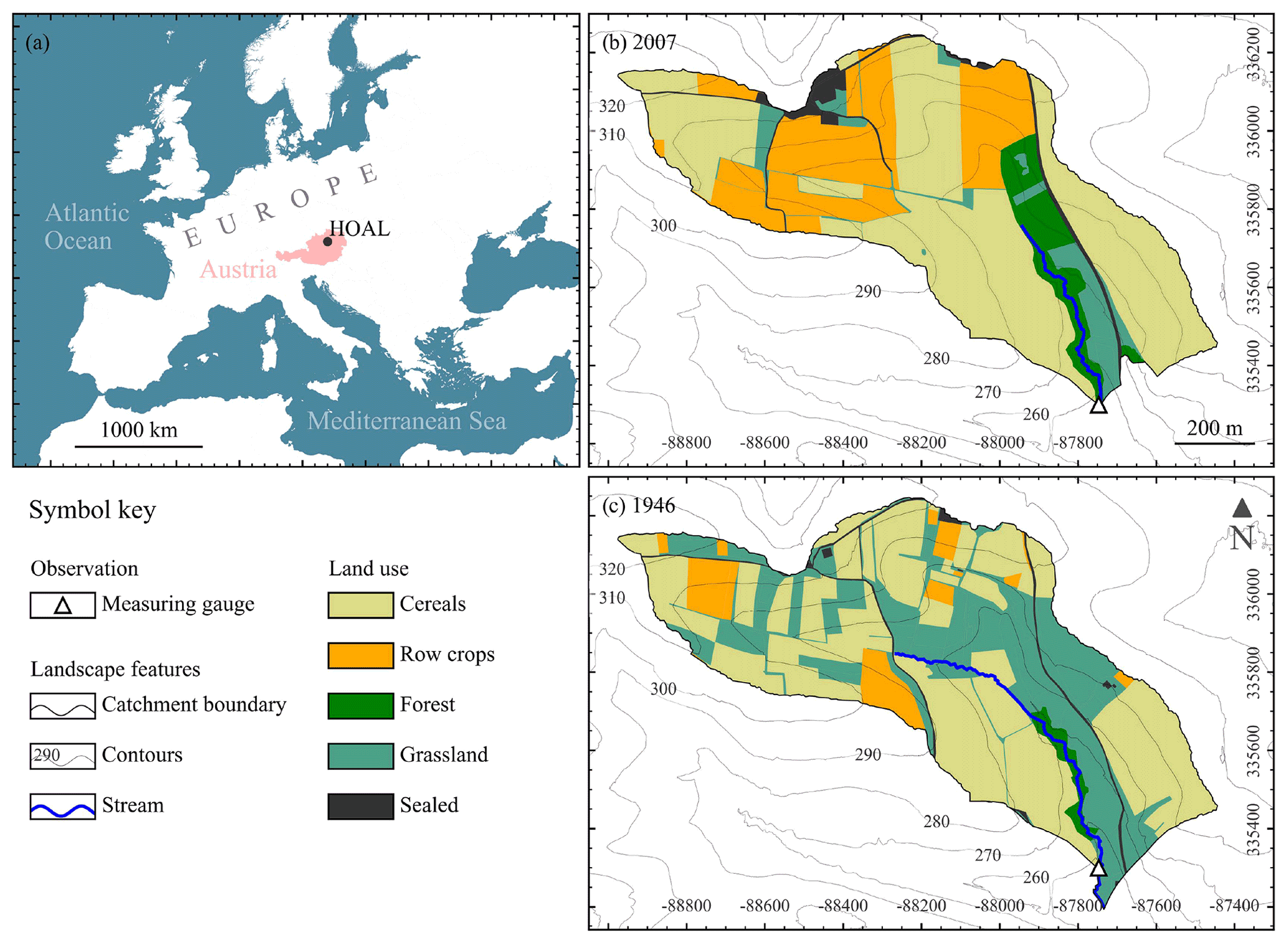
Figure 1(a) The geographical location of the HOAL catchment in Petzenkirchen, Austria, and within Europe. The parcel structure and land use in the HOAL catchment for (b) 2007 and (c) 1946. (Coordinates as per EPSG: 31256 – MGI/Austria GK East, in meters.)
2.2 Data availability in the catchment
Both discharge (Q, L s−1) and suspended sediment concentration (C, mg L−1) have been measured at the catchment outlet periodically since the 1940s. A data set of discharge and sediment concentration was available for the period from 1945 to 1954. After that, measurements were stopped and were not started again until 1990. Therefore, data records for the period from 1946 to 1954 (Period I) and for the period from 2002 to 2017 (Period II) were used for this analysis. In Period II, the stream gauge was relocated. However, the difference in catchment size is very small (around 200 m2). This is indicated by the different discharge gauge locations in Fig. 1. Due to technological advances, the measurement method of both Q and C also changed between the two periods: in Period I, discharge was registered by a Thomson weir and a paper chart recorder, whereas it was registered by a H Flume and a pressure transducer in Period II. Thus, high-temporal-resolution 1 min data for discharge were available for both periods. Sediment concentrations were measured manually every 3–4 d in Period I, whereas an automatic method (i.e., equal-discharge-increment sampling) and additional manual sampling were applied in Period II. Daily precipitation and 5 min rainfall intensities were available for both periods, but 5 min rainfall intensities were only available during the growing season for Period I.
We used parcel-based land use data from 1946 to 1949 and from 2007 to 2012, representing Period I and Period II land use, respectively. Land use categories were agricultural land, including crop type, grassland, forest, roads, and settlements (i.e., paved area). We defined a parcel as a continuous area of land with a single crop type. Parcel boundaries were specified according to the cadastral map and aerial photographs. In Period II, these boundaries were also visually inspected. Figure 1 depicts the geographic catchment location as well as the parcel structure and land use for a specific year in each period.
2.3 Data analysis
2.3.1 Changes in rainfall erosivity and flow regime
The erosive potential of rainfall events was quantified by the R factor of the Revised Universal Soil Loss Equation (RUSLE), which is defined as the product of the kinetic energy of a rainfall event and its maximum 30 min intensity, using the Rainfall Intensity Summarization Tool (RIST) (USDA-Staff, 2019) according to
Here, EI30 is the annual R factor (MJ mm ha−1 h−1), calculated as the sum of single-event R factors; Ei is the total kinetic energy for a single event (MJ m−2); I30 is the maximum rainfall intensity in 30 min within a single event i (mm h−1); and m is the number of events per year.
We assumed erosivity density (i.e., EI30 divided by event precipitation) to be a particularly relevant climatic indicator of the soil erosion process and catchment sediment yield, as it is calculated as a combination of the rainfall kinetic energy and maximum rainfall intensity of rain events. These are commonly considered as the relevant parameters of rain to trigger soil erosion. Thus, we tested if the means of the monthly erosivity density (ED) were significantly different between Period I and Period II using a t test. Due to the absence of rainfall intensity measurements, we could not directly calculate ED for the months of the dormant season (November–March) in Period I; instead, we calculated ED from a relationship between EI30 and the monthly rainfall of Period II, assuming that the relationship was sufficiently temporally invariant over the investigated periods. Erosivity density is very low during the dormant season. The mean ED was 0.66 ± 0.21 and 2.54 ± 2.43 MJ ha−1 h−1 for the dormant season and the growing season of Period I, respectively, whereas it was 0.42 ± 0.11 and 1.87 ± 1.35 MJ ha−1 h−1 in Period II, respectively (Fig. 3a). Thus, the error arising from the use of this relationship is expected to be small.
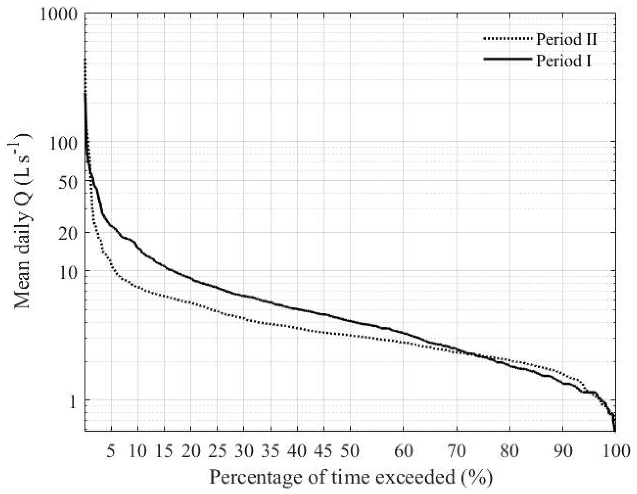
We also compared daily flow duration curves to understand whether hydrological regime change has influenced the flow transport capacity and sediment regime change. Following the definitions of Smakhtin (2001), we compared low-flow-rate (Q70 %), high-flow-rate (Q10 %), and median-flow-rate (Q50 %) quantiles for the two periods.
2.3.2 Sediment regime analysis
To analyze the sediment regime, we first estimated sediment loads for the different periods. After calculating sediment rating curves (SRCs) for Period I and Period II, using the data pairs of Q and C measurements, daily sediment load was estimated (see Eq. 2) by combining the measured high-resolution data (1 min) for Q with the derived SRC for each period. For further analysis, the daily sediment load was aggregated either by month or year.
where Y is the sediment load within a day (kg d−1), Qi is the observed discharge at time step i (L s−1), is the estimated sediment concentration at time step i (mg L−1), and Ti (s) is the elapsed time between time step i and the next time step i+1. The statistical differences of sediment loads either between seasons or between periods were examined using a t test.
Following a commonly used approach (Asselman, 2000; Warrick and Rubin, 2007; Sheridan et al., 2011; Vaughan et al., 2017; Khaledian et al., 2017), the SRCs were assumed to follow a power-law function, which was fitted by least squares regression:
where C is sediment concentration (mg L−1), Q is discharge (L s−1), and a and b are regression coefficients. The coefficient a is usually associated with easily transported intensively weathered materials and may vary over 7 orders of magnitude (Syvitski et al., 2000). The parameter b represents the capacity of the stream to erode and transport sediment, reflecting how sediment concentration is nonlinearly related to streamflow (Sheridan et al., 2011; Fan et al., 2012). It typically varies from 0.5 to 1.5 and rarely exceeds 2. Sometimes b is also regarded as a measure of the quantity of newly available sediment sources (Vanmaercke et al., 2010; Guzman et al., 2013).
Considering that data records were registered with different intensity for periods I and II (see Sect. 2.2), for the sake of consistency, we used monthly averages, as in other studies (Syvitski and Alcott, 1995; Sheridan et al., 2011; Hu et al., 2011), to construct SRCs. We assumed that monthly averages could reflect a varied hydrological and/or sediment response to seasonally prevailing weather characteristics, such as dry periods or convective storms (Sheridan et al., 2011).
We chose arithmetic means of the observations to represent the monthly Q and C values. These monthly averages were pooled together and then grouped into the growing season of Period I (Period I_G), the dormant season of Period I (Period I_D), the growing season of Period II (Period II_G), and the dormant season of Period II (Period II_D), respectively. For each of these four periods, we fitted SRCs.
We analyzed the fitted SRCs and used two strategies to evaluate whether and how the sediment regime changed between these periods. Besides directly comparing the slopes of the four seasonal SRCs using an ANCOVA (analysis of covariance) analysis with the log-transformed discharge as independent variable, we also fitted the SRC for each specific year's season and plotted the regression coefficients a against their corresponding b to evaluate a possible sediment regime shift during periods I and II.
The latter framework was adapted from Thomas (1988) and was also employed by Asselman et al. (2000) and Fan et al. (2012) to examine differences in sediment regimes between spatially different sites. Moreover, Sheridan et al. (2011) used the framework to reveal post-fire temporal shifts in a sediment regime. Thomas (1988) suggested that time-based sampling methods (either random sampling or systematic sampling) preferentially use observations of relatively small discharges to fit an SRC. This tends to reduce the slope and increase the intercept of an SRC (see point C in Fig. 2b). In contrast, flow-based automatic sampling methods, such as equal-discharge-increment sampling, preferentially use observations of relatively large discharges. Thus, they tend to cause a reversed pattern of a and b (i.e., increase the slope and decrease the intercept of SRC; see point A in Fig. 2b). However, irrespective of sampling practices, the pairs of data points (a–b) will likely be allocated along a straight line if sediment transport regimes are similar. The reason for the a–b pairs lying nearly on a straight line is mainly due to a mathematical property: the slopes could be expressed by a linear function of the intercepts with the coordinates of the common point (Thomas, 1988). Therefore, for years with similar means of log Q and log C, the SRCs will pass through one common point O (Thomas, 1988; Syvitski et al., 2000; Desilets et al., 2007; Sheridan et al., 2011). This common point O (Fig. 2a) is usually interpreted to reflect temporally invariant catchment characteristics, such as relief, drainage area, and drainage density, whereas the variation in the slope of SRCs (Fig. 2a) is interpreted to reflect temporally dynamic characteristics, such as average or maximum discharge and sediment availability (Asselman, 2000). The coefficients a are usually inversely linearly related to b (Thomas, 1988; Syvitski et al., 2000; Desilets et al., 2007), and each point is representative of a period (or a catchment). If sediment transport regimes are similar between periods (catchments), the points will be plotted on the same line (such as A, B, and C in Fig. 2b), with points A in Fig. 2b (upper left) often exhibiting steeper sediment rating curves than points C (lower right). As for the different lines in Fig. 2b, the lower ones, characterized by points A', B', and C', represent situations with most of the annual sediment load being transported at relatively low-flow discharges, whereas the higher ones, characterized by A, B, and C, represent situations with suspended sediment being mainly transported at high streamflow. Compared with a direct evaluation of rating curves, relating coefficient a to exponent b is more conductive to revealing the temporal evolution of a sediment regime (Syvitski et al., 2000; Desilets et al., 2007). The change in the relationship of the coefficients a against b between the periods was also examined using an ANCOVA.

Figure 2Schematic showing (a) how sediment rating curves (SRCs) may rotate around a common point and (b) how exponents b of the SRCs relate to coefficients a. Lines A, B, and C on the left are SRCs of different periods (e.g., years) sharing a similar common point O. Once sediment regimes shift due to changes in catchment characteristics (change in drainage density, drainage area, and topography), the common point O changes to point O', and the linear relationship between a and b of the SRCs also exhibits a shift. The schematic is based on log C= log a + b ⋅ log Q (Eq. 3).
To account for uncertainties in the fitted SRCs during each period, we additionally established theoretical sediment rating curves (tSRCs) using the following process:
- i.
For each period (i.e., Period I_G, Period I_D, Period II_G, and Period II_D), we carried out random sampling of log a (n= 500, “sample” package in R), assuming that the samples of the coefficient of log a follow normal distributions, which was examined with a Kolmogorov–Smirnov test of normality (mean = 1.02, SD = 2.01, n= 44, p < 0.05).
- ii.
Given the set of the 500 sampled values of log a, we generated a set of b values according to the previously established linear relationship between log a and b.
- iii.
Given a set of specified Q values, we derived 500 tSRCs for each period, corresponding to the paired log a and b samples.
- iv.
Using these tSRCs, we calculated the 50th percentile, the 5th percentile, and the 95th percentile for each period to estimate the uncertainties of the sediment rating curves.
The tSRCs of the periods were also used to quantify the effect of land consolidation, i.e., the change in parcels' structure and size (Parcel_effect) and the effect of land use and land cover changes (LUCC_effect). Vegetation usually plays a minor role in the dormant season due to the absence of a dense vegetation cover on arable land and little erosive rainfall (Madsen et al., 2014; Salesa and Cerda, 2020; Hou et al., 2020). Therefore, landscape structure in the dormant season was considered a dominant factor for water and sediment transfer across the land surface and, thus, for runoff production and sediment production (Sharma et al., 2011; Devátý et al., 2019). Therefore, we hypothesized that the total change in sediment yield (Total_effect) resulted from land cover change (LUCC_effect), land structure change (Parcel_effect), and climate change (Climate_effect). As the area of our catchment is only 0.66 km2, no obvious change was found in the shape of the small stream for the two periods. Stream sediment resuspension is rather small (Eder et al., 2014); therefore, the contribution of bank erosion was not taken into account. The effects of land cover and land structure change was quantitatively separated according to the seasonal differences in the tSRCs after determining the climate change effect. Specifically, we assumed that the shift in sediment regime from Period I_D to Period II_G was representative of the Total_effect (Eq. 4), and the shift in sediment regime between Period I_D and Period II_D was mainly due to land consolidation (Parcel_effect) (Eq. 5). Thus, the LUCC_effect could be estimated according to Eq. (6) if the Climate_effect was insignificant (Sect. 3.1). The contributions of the Parcel_effect and the LUCC_effect to the Total_effect were estimated according to Eqs. (7) and (8), respectively.
3.1 Changes in climate and flow regime
Because climate change is often found to be responsible for hydrological change (e.g., Kelly et al., 2016; Wang et al., 2020), we compared the erosivity density (ED) and monthly precipitation (P) of the two periods to examine whether climate affected the variation in the sediment regime in the catchment (Fig. 3). The mean monthly ED values in the growing season were 2.37 ± 1.38 and 1.84 ± 0.86 MJ ha−1 h−1for periods I and II, respectively (Fig. 3a). No significant difference (p > 0.05) was found between the two growing seasons. Mean monthly ED in the dormant seasons significantly decreased from Period I (0.66 ± 0.21) to Period II (0.42 ± 0.11 MJ ha−1 h−1). A t test suggests that there was no significant (p > 0.05) difference in mean monthly P between Period I and Period II in the dormant season nor the growing season (Fig. 3b). The mean monthly P was 50 ± 33 and 76 ± 54 mm for the dormant and growing season of Period I, respectively, and it was 53 ± 29 and 79 ± 47 mm for the two respective seasons of Period II. The decrease in ED during the dormant season of Period II and the insignificant change in monthly P suggest that climate change between Period I and Period II was not responsible for an increased sediment load (see Sect. 3.3). It should be noted that processes related to snow play a minor role in the catchment, as it is considered a lowland catchment and is located in a region with very small amounts of snowfall (about 10 % of annual rainfall). Thus, a possible change in the proportion of snowfall in precipitation during the winter season of periods I and II was not accounted for when addressing the impact of climate change on sediment load.
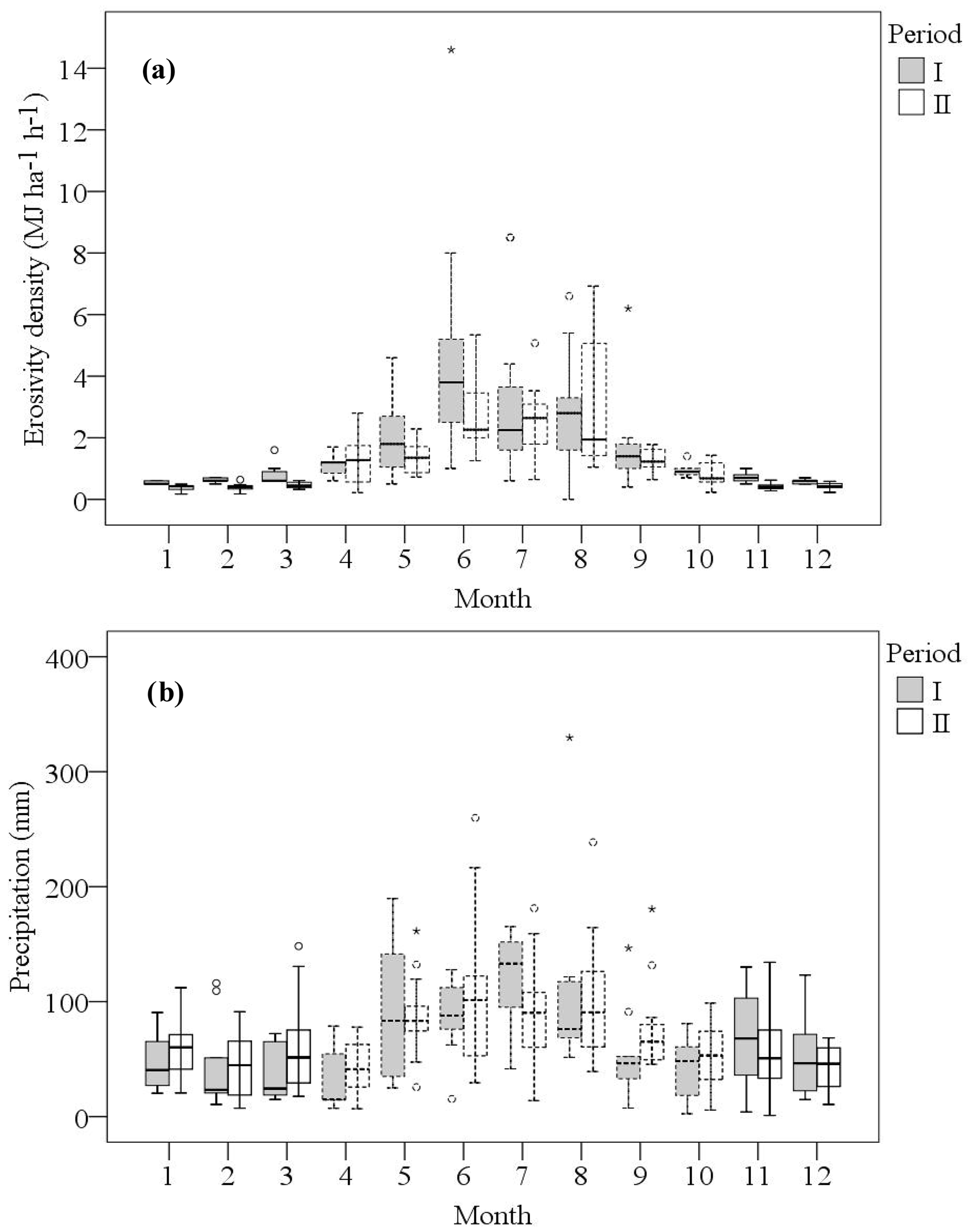
Figure 3Monthly erosivity density (a) and monthly precipitation (b) for periods I and II. The bars with a dashed outline represent the growing seasons (April–October), the bars with a solid outline denote the dormant seasons (November–March), the whiskers indicate the range between the minium and the maximum, and the asterisks indicate the outliers.
Streamflow in Period I was higher than during Period II: the mean annual streamflow was 188 and 146 mm yr−1 for periods I and II, respectively. Daily flow duration curves for both periods are displayed in Fig. 4. A t test suggests that they are significantly different (p < 0.05). The Q70 % low flow of the two respective periods was 2.7 and 2.4 L s−1, the Q50 % median flow was 4.0 and 3.1 L s−1, and the Q10 % high flow was 10.7 and 7.5 L s−1. The decreased flow regime of Period II, which is probably due in part to increased evapotranspiration over the past decades (Duethmann and Blöschl, 2018), indicates that streamflow cannot account for the observed increased sediment load during this period; otherwise, increased streamflow would be expected in Period II.
3.2 Change in land use and land organization
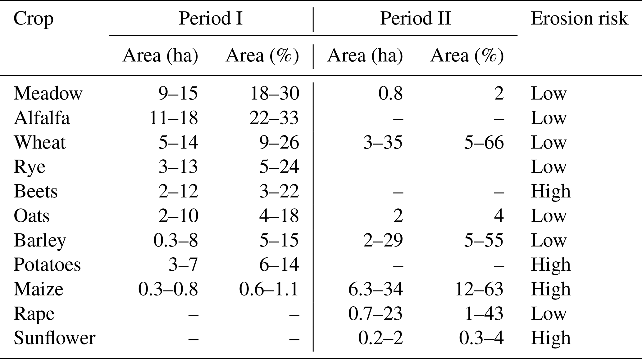
Table 1 shows how land use changed between the two periods. During Period I, cropland and grassland accounted for 73 %–82 % (varying between years) and 14 %–22 % of land use, respectively. However, due to agricultural intensification, cropland increased to around 82 % in Period II, at the expense of a decreasing share of grassland. Forest, including sparse forest, accounted for 1.8 % of land use during Period I but increased considerably by Period II to around 11 %. The increase in cropland and forest suggests higher rates of evaporation and transpiration and, consequently, less streamflow, which is in line with the previously examined trends of streamflow dynamics. Upon further analysis of the land use classes of arable land, a substantial change was also found for the crop types, with the crops at low risk of soil erosion being replaced by crops that exhibit a high soil loss potential. This was particularly true for maize. In addition, the diversity of crops decreased considerably (Table 2). This shift towards agricultural uniformity likely acts as a land structure effect. A loss of crop type heterogeneity increases the probability that different fields are managed with the same crop. In this case, even smaller fields may behave similarly to larger fields in terms of sediment production.
Table 1Parcel and land use statistics for periods I and II: Period I represents land use for the years 1946–1949, and Period II represents land use for the years 2007–2012. N is the number of parcels for a given land use, density is the number of parcels per hectare, and mean size represents the mean area of parcels with a particular land use.
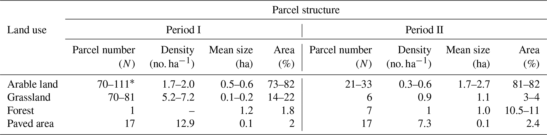
* The number of parcels varied with year during a period.
Table 2Crop statistics of arable land for periods I and II: Period I represents crop statistics for the years 1946–1949, and Period II represents crop statistics for the years 2007–2012. The erosion risk for a particular crop is classified as high or low according to the classification of management using the RUSLE. The statistical values represent the ranges of the area for each crop during periods I or II.
Besides the change in land use, the parcel structure of the catchment also changed (Table 1). This change was related to a land consolidation plan issued in Austria in 1955 (Devátý et al., 2019) and a massive trend toward agricultural industrialization that evolved after 1945 (mainly referring to the massive application of advanced machinery and fertilization technologies that started in the 1950s). During Period I, arable land was fragmented across many small parcels, with a mean parcel size of between 0.5 and 0.6 ha and a resulting parcel density (number of parcels per hectare area) of between 1.7 and 2.0 ha−1 in different years. In Period II, these values increased considerably to mean parcel sizes of between 1.7 and 2.7 ha and parcel densities of between 0.3 and 0.6 ha−1. Similarly, the mean parcel size and parcel density of grassland during Period I were 0.13–0.17 ha and 5.2–7.2 ha−1, respectively; this changed to respective values of 1.06 ha and 0.9 ha−1 in Period II. As parcel structures have been identified as influencing sediment loads, mainly due to the boundary effects (e.g., Baudry and Merriam, 1988; Takken et al., 1999; Phillips et al., 2011), the substantial decrease in the parcel density of the catchment in Period II was expected to have affected the sediment load as well.
3.3 Change in the sediment transport regime
3.3.1 Direct comparison of the fitted SRCs
Figure 5 shows the fitted sediment rating curves (p < 0.05) for both periods. A t test suggests that the slopes of the regression lines are significantly different between the dormant seasons and growing seasons (p < 0.05). Although the rainfall erosivity of Period II_G was similar to that of Period I_G (Fig. 3a) and the streamflow of Period II was generally lower than that of Period I (Fig. 4), the fitted SRC of Period II_G was steeper than that of Period I_G (Fig. 5a), with coefficient b values of 0.3 and 1.6 for Period I_G and Period II_G, respectively (Table 3). The fitted SRC of Period II_D demonstrated a faster response of the sediment concentration to increasing flow compared with that of Period I_D (Fig. 5b), with coefficient b values of 0.8 and 1.7 for Period I_D and Period II_D, respectively. However, the rainfall ED in Period II_D was generally lower than that of Period I_D (Fig. 3a). This suggests the lower probability of a substantial increase in sediment availability. These results indicate that neither changes in rainfall erosivity nor the hydrological regime could explain the increase in sediment dynamics.
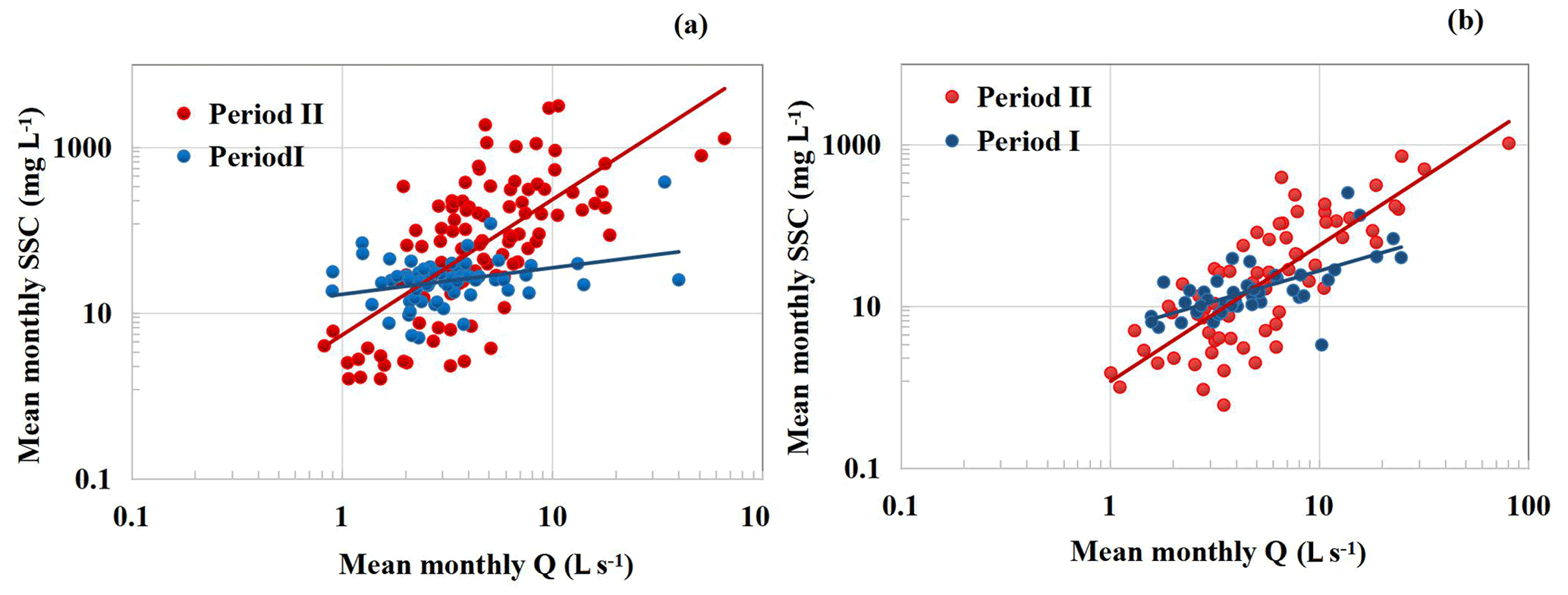
Figure 5Sediment rating curves for (a) the growing seasons and (b) the dormant seasons during the two time periods. Each point represents a monthly mean observation.
Table 3Parameter values for the coefficients of the SRCs for different periods and seasons according to Eq. (3).

3.3.2 Relationship between coefficient a and b
The changing steepness of a fitted SRC does not necessarily imply a change in the sediment regime, as the slopes of fitted SRCs are sometimes affected by catchment size or the distribution of samples (Asselman, 2000). To minimize possible interference from other factors when identifying variations or shifts in the SRCs, we investigated the relationship between coefficients a and b of the SRCs. Figure 6 shows the coefficients log (a) plotted against b for the four investigated time frames. Interestingly, the data points of both periods I and II are more concentrated in the lower-right part of the graphs for the growing season (Fig. 6a). A different pattern of log (a) against b was found for the dormant season (Fig. 6b): the data points of Period I were concentrated in the lower-right area (blue points), but the points for Period II were more concentrated in the upper-left area.

Figure 6Relationship between coefficients a and b for (a) the growing season and (b) the dormant season during Period I (blue) and Period II (red), respectively. log (a) on the x axis represents the decadal logarithm. The arrows represent the shift in the sediment regime between Period I and Period II (see text below). All regressions are significant at p < 0.05.
According to Asselman (2000), a shift in the sediment regime means an alteration of either soil erodibility and/or the erosive power of the river. In Fig. 6, we found that the regression lines of periods I and II are different. The intercepts of the regression lines are significantly different for the growing seasons (p < 0.05, Fig. 6a). The slopes of the regression lines for periods I and II were −1.60 and −0.94 in the growing season (Fig. 6a), and −1.58 and −0.80 in the dormant season, respectively (Fig. 6b). The upward shift in the line at log (a), larger than around 0.6, suggests that most of the sediment was transported at relatively high flow rates in Period II. As climate change was not responsible for the increased hydrological regime (see Sect. 3.1), we mainly attribute this shift to the increase in hydrological connectivity, such as flow path density and flow length, and to a change in land use and land cover statistics.
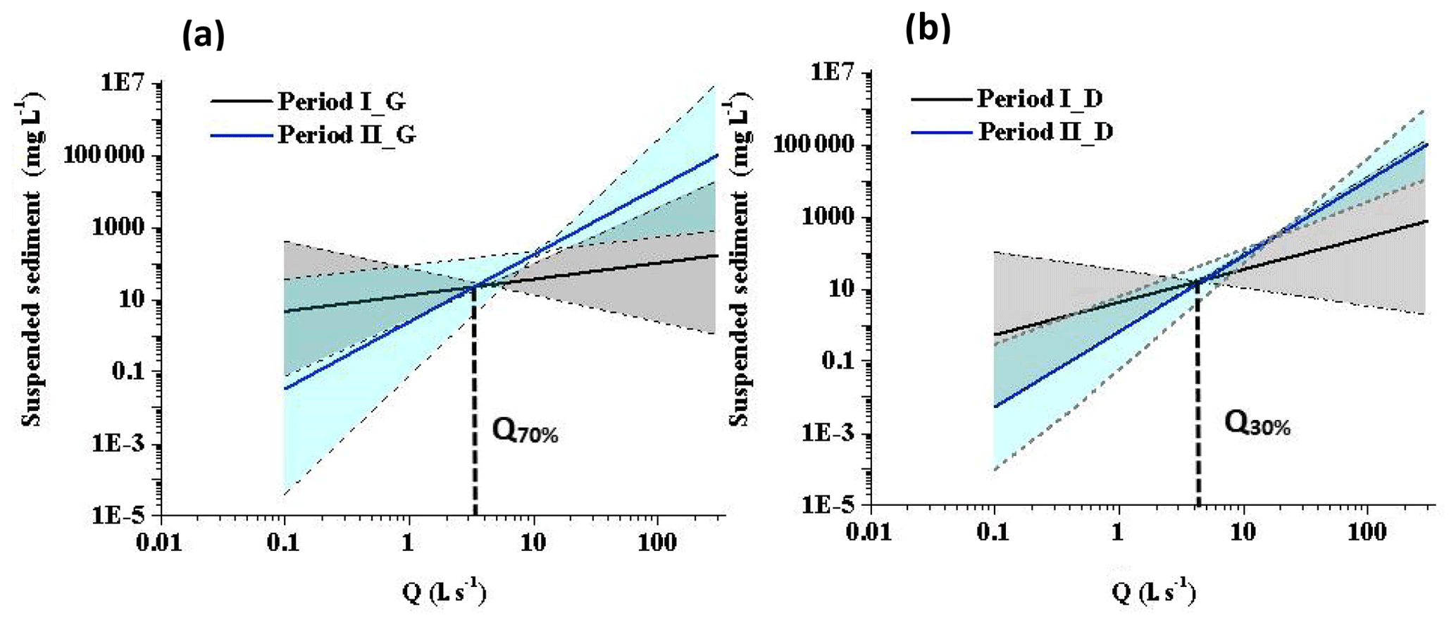
Figure 7Theoretical sediment rating curves (tSRCs) for the growing seasons (a) and the dormant seasons (b) of Period I and Period II. Solid lines denote the 50th percentile of the tSRCs for each period (i.e., tSRC50 %). The gray area denotes the range of the predicted tSRCs composed of the 5th and 95th percentiles (i.e., tSRC5% and tSRC95 %, respectively). Q30 % and Q70 % represent the flow conditions of 3.9 L s−1 and 2.0 L s−1, respectively.
Figure 7 displays the theoretical sediment rating curves (tSRCs) with their uncertainties for the different periods and seasons. At a given Q higher than approximately Q70 %, sediment concentrations in Period II_G were higher than those in Period I_G (Fig. 7a), whereas sediment concentrations were not different for flow rates below the abovementioned value. The increased sediment concentrations in Period II_G are in line with the observations of the sediment load of Period II_G (6.3 ± 32.5 t per month), which is largely enhanced compared with that of Period I_G (0.4 ± 0.9 t per month; see Table 4). Sediment concentrations were less different between the dormant seasons of Period I and Period II at flow rates lower than Q30 % (Fig. 7b), which is also reflected by the insignificant (p > 0.05) difference in sediment loads between Period I_D and Period II_D (0.6 ± 1.1 and 3.2 ± 14.0 t per month, respectively). However, an ANCOVA suggests that the derived tSRC50 % values were significantly different (p < 0.05) between the two periods, both in the growing seasons and dormant seasons. This enables us to estimate the LUCC_effect and Parcel_effect according to the derived tSRCs.
Table 4Monthly mean sediment loads and associated standard deviations of different periods.
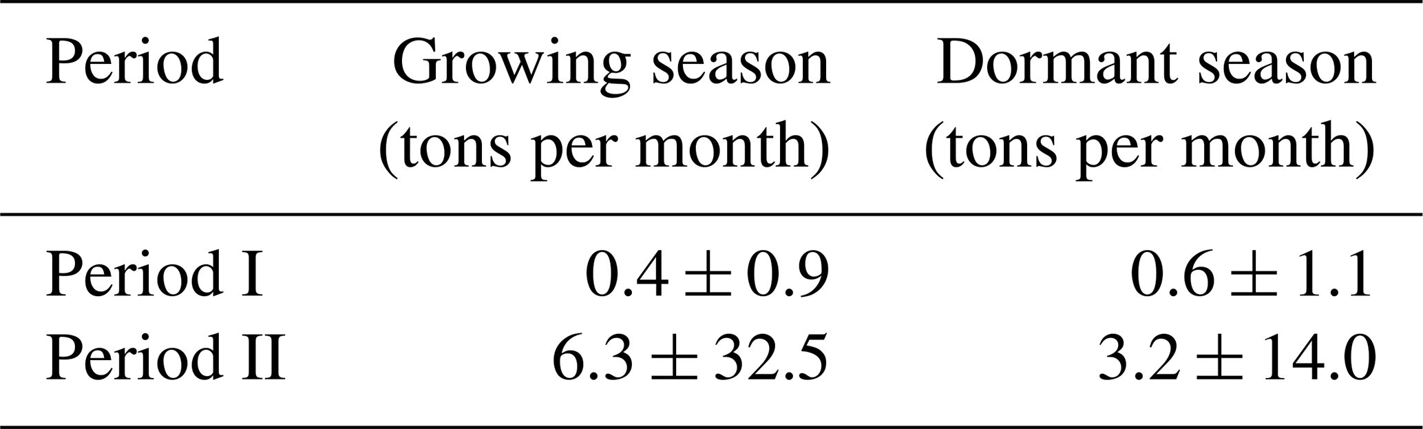
Note that the estimates are based on Eq. (2).
3.4 Parcel_effect vs. LUCC_effect
Figure 8 demonstrates the dynamic contributions of land structure change (Parcel_effect) and LUCC (LUCC_effect) to sediment concentrations with increasing flow. Land structure change and the increase in cropland as well as a shift to crops with a higher risk of erosion explain the increase in sediment yield. However, the extent of their contributions to this increase differ. Generally, with higher flow rates, the contribution of the LUCC_effect gradually decreased, whilst the contribution of the Parcel_effect increased. The Parcel_effect accounted for more than 50 % of the Total_effect after the flow rate exceeded approximately 20 L s−1 (i.e., Q2 %) (Fig. 8), exhibiting a dominant role in sediment production. This opposite trend of the relative contributions of the LUCC_effect and the Parcel_effect suggests that, although land structure change and LUCC both have unbeneficial effects on erosion control, their hydrological consequences may be different. Land structure change probably explains much of the variation in sediment load under high-flow conditions.
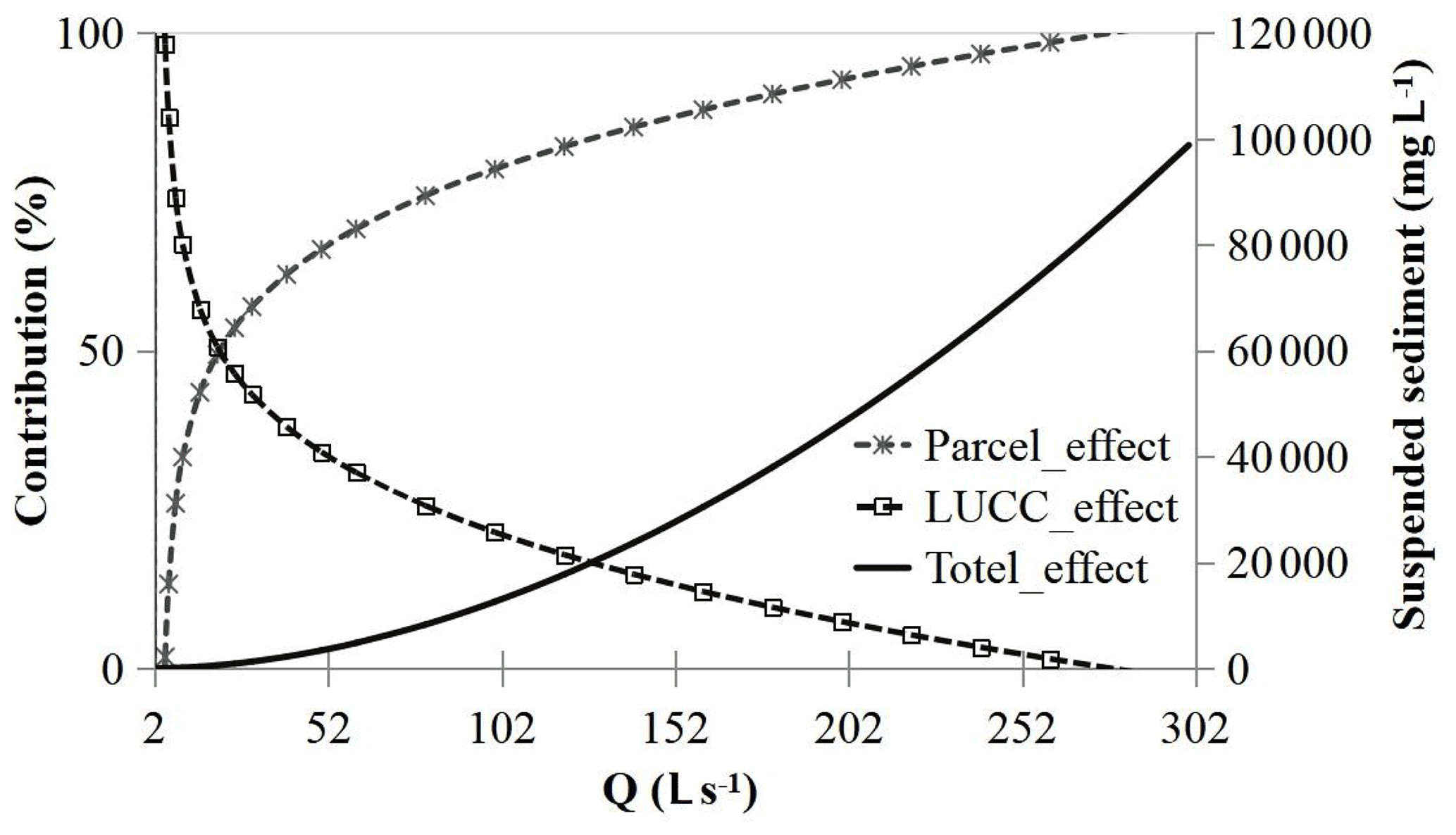
Figure 8The contribution of the Parcel_effect and LUCC_effect to the Total_effect across various flow rates. The Total_effect (Eq. 4) is displayed in terms of suspended sediment concentration. The Parcel_effect and LUCC_effect were estimated using Eqs. (5) and (6), respectively; their contribution to the Total_effect was estimated using Eqs. (7) and (8), respectively.
Unlike the situation with high flow rates, the Total_effect showed an almost zero value at flow rates less than approximately 2 L s−1 (i.e., Q70 %), suggesting no difference in sediment load between periods I and II under low-flow conditions. The increase in the sediment concentration at flow rates of 2 L s−1 up to around 20 L s−1 seemed to be mainly caused by the changes in LUCC in Period II, as the contribution from the LUCC_effect was consistently higher than that of the Parcel_effect.
One may note that forest land cover increased considerably from Period I to Period II. We hypothesize that, although a beneficial effect of forest increase (up to a total of 11 % of the catchment) may have appeared in Period II, it was easily offset by the negative effect of crop land changes, particularly the increase in row crops that are generally at high risk of erosion. This contributed substantially to sediment yield compared with other land uses and other crop types (Kijowska-Strugała et al., 2018).
The industrial intensification of agriculture implemented over the last 70 years has raised considerable concerns regarding erosion and sediment loading of rivers (e.g., Bakker et al., 2008; Chevigny et al., 2014). However, with global climate warming, the different contributions of LUCC, land policy adjustments (i.e., land structure changes), and climate change affecting the sediment load remain unclear. This paper aims at evaluating the relative roles of climate change, LUCC, and land structure changes for sediment production, particularly at different flow rates.
4.1 Change in sediment load between the two time periods
We found that the sediment load increased almost 6 fold from Period I to Period II. This finding is supported by estimates of the management factor (C factor) and the slope and slope length factor (SL factor) of the RUSLE for Period I and Period II (Fiener et al., 2020). The C factor integrates changes in land use and crop statistics; thus, it directly corresponds to changes in LUCC. The SL factor integrates parcel slopes and parcel sizes. Considering that the slopes in the HOAL did not change between the two periods, the SL factor may be used as direct indicator of changes in land structure. While the mean C factor of the HOAL catchment increased from 0.16 in Period I to 0.33 in Period II, the SL factor increased from 0.76 to 0.96. Added together, the changed values of these two factors increased the theoretical soil loss within the catchment by over 150 %. This value is smaller than the changes observed; however, it should be noted that the RUSLE has not been designed to account for sediment loads of catchments but instead to estimate field-scale soil loss within catchments. This may explain the observed differences to a certain extent.
4.2 The potential interference of different sampling methods
Due to technical advancement over the long investigation period, different sampling methods (i.e., grab sampling and automatic equal-discharge-increment sampling) were used in this study for periods I and II. This may affect both the rating curve estimation and the sediment load estimation (Harmel et al., 2010; Thomas, 1988).
To test a potential influence that may result from the different sampling frequencies in the two periods, we resampled the data set of Period II. We randomly selected repeated subsamples (n= 10) of the Q−C observations of Period II with equal sample size to that of Period I. With each of the resampled data sets, we calculated SRCs. Combined with the flow data, the derived 10 SRCs were then used to calculate a mean annual sediment load. Comparing the mean annual sediment load from the resampling (62.4 ± 10.2 t yr−1) to that of the original data set (60.0 ± 140.0 t yr−1) resulted in an insignificant difference, suggesting that the different sampling strategies of periods I and II did not affect the results.
Further support to the validity of our results is provided by Groten and Johnson (2018), who suggested that the bias of different sampling strategies might be small for sediment with very fine textural composition. In our study catchment, the topsoil of the catchment is very fine textured, consisting of 75 % silty loam, 20 % silty clay loam, and 5 % silt according to the USDA soil classification (Picciafuoco et al., 2019).
4.3 The dynamic relevance of land consolidation in controlling sediment load
Climate change in terms of both monthly erosivity density (ED) and precipitation (P) was not responsible for the increase in sediment load; instead, the increase could be explained by LUCC and land structure changes. This finding is particularly important in regions in which a strong intensification of agricultural management has taken place during the last decades. The relative contributions of LUCC and land structure changes varied with streamflow. For flow conditions below around 5 L s−1 (i.e., Q20 %), land structure change had no apparent adverse effect on erosion; however, with increasing flow, the contribution to sediment load increased continuously, leading to a dominant role at high flow rates. This finding is partially in line with David et al. (2014) and Cantreul et al. (2020). The aforementioned studies reported that landscape structure was less important for soil erosion than LUCC under normal flow conditions. However, they did not investigate whether the effect of landscape structure showed a dynamic behavior with increasing flow. In contrast, the LUCC_effect, i.e., the increase in crops with a high erosion risk and the change in land use, continuously affected the sediment load, with gradually decreasing importance under high-flow conditions. Similar results were reported by Vaughan et al. (2017), who showed that the sediment concentration under low- and median-flow conditions was considerably associated with a change in catchment characteristics, primarily land use and land cover. Although the role of LUCC was dominant for flow conditions less than Q20 %, its contribution to the total annual sediment load was small. More than 75 % of the total sediment load was transported during a small number of events (25 events in Period I and 8 events in Period II), and all events had flow rates above 15 L s−1 (approximately at Q13 % in Period I or Q4 % in Period II), which underlines the importance of land structure for sediment loading.
The dynamic relevance of LUCC and land structure changes in sediment production is associated with the processes and mechanisms controlling overland flow as a transport agent for sediment (e.g., Sun et al., 2013; El Kateb et al., 2013; Nearing et al., 2017; Silasari et al., 2017; Kijowska-Strugała et al., 2018). A change in the types of land use and the crops used (LUCC) implies alterations of surface characteristics, such as aboveground structure morphology, litter cover, organic matter components, root network (Gyssels et al., 2005; Wei et al., 2007; Moghadam et al., 2015; Patin et al., 2018), and soil properties (Costa et al., 2003; Moghadam et al., 2015). These properties influence the protective role of vegetation in soil detachment, the flow capacity to transport sediment particles, and runoff flow paths to the stream channels (Van Rompaey et al., 2002; Lana-Renault et al., 2011; Sun et al., 2018). The protective effects tend not to linearly increase with increasing surface runoff. Accelerated discharge and stronger scouring effects of upslope discharge might impair the protective role of vegetation (e.g., Zhang et al., 2011; Santos et al., 2017; Bagagiolo et al., 2018; Yao et al., 2018; Wang et al., 2019). Vegetation usually exhibits a smaller interception capability at high rainfall intensity, resulting in enhanced splash erosion and availability of mobile soil particles (Cayuela et al., 2018; Magliano et al., 2019; Nytch et al., 2019). However, the decreasing contribution of the LUCC_effect does not directly imply an absolute decrease in the magnitude of the LUCC_effect. The absolute change in the sediment concentration resulting from LUCC reveals an increasing trend as flow rates increase. Thus, the contribution of the LUCC_effect represents the relevance of LUCC in erosion control compared with the change due to land structure. The magnitude of the LUCC_effect probably depends mainly on where within the catchment the LUCC is changed and how the proportional area of various land uses changes. We will address this topic in future analyses.
Unlike land cover and land use change, landscape structure is usually combined with other catchment properties, such as slope characteristics and soil properties (Gascuel-Odoux et al., 2011) as well as additional erosion and transport factors (Verstraeten and Poesen, 2000). These factors exert a more complicated influence on erosion. For example, the effect of landscape structure on soil erosion may be identified on moderate slopes, whereas it may be concealed by on-site severe soil erosion on steep slopes (Chevigny et al., 2014). However, the key process for erosion control is the fact that landscape elements and their structural position (i.e., parcel structure, field boundaries, hedges, and similar) alter hydrological connectivity between the land and water. This is particularly true when the land cover on both sides of boundaries is different (Van Oost et al., 2000). Reducing parcel size and heterogeneity significantly increases hydrological connectivity and results in a substantial off-site damage effect, irrespective of on-site erosion of the investigated land use (Boardman et al., 2019; Devátý et al., 2019). Under low- and median-flow conditions, surface runoff and sediment may arrive to a lesser extent at field boundaries due to efficient interception effects of the vegetation cover. This may explain the identified dynamic relevance of land structure change in sediment load found here.
Climate change, land use and land cover change, and other human-associated activities are widely regarded as potential agents driving hydrological change. Understanding the relevance of each of these agents in the hydrological cycle is critical for implementing adaptive catchment management measures and addressing climate change. Although very significant climate change influences have been identified for certain components of the hydrological cycle in the last decades, we found that climate change, expressed as changes in rainfall erosivity and precipitation, cannot explain the increased sediment production between 1946–1954 and 2002–2017 in the investigated catchment. Instead, both LUCC and land structure change played important, dynamic roles in erosion and sediment production.
The relevance of land use and land cover change vs. land structure change varied dynamically with changing flow conditions. The reduction in parcel density undoubtedly increased the sediment load, particularly at higher flows due to the decreased capacity for trapping sediment particles between parcels and increasing flow lengths inside parcels. Unfavorable land use or land cover change increased the sediment load under most flow conditions, although the relevance of this process decreased at high or very high flow rates. Therefore, when addressing soil conservation measures at the catchment scale, the distribution of fields, land structure, and vegetation cover should be simultaneously considered. Such a strategy would be conducive to dealing with the risk of soil erosion at different flow rates. Land use policy adjustments resulting from technological development have been vital for dealing with food security issues in the past. However, we are currently experiencing the negative influence of these adjustments on the hydrological cycle. Therefore, rather than focusing solely on climate change, we need to pay increased attention to anthropic management activities to effectively counteract their negative impact on hydrological change.
The pieces of code that were used for all analyses are available from the authors upon request.
The data sets that have been analyzed in this paper are available from the authors upon request.
SW led the data analysis, drafted the manuscript, and revised the manuscript. BS helped to revise the manuscript and coded the resampled part of the data set for Period II. CK was responsible for data collection and data preparation for Period I. ES contributed to figure creation, manuscript revision, and data provision for Period II. KS and YL helped with data processing and statistical evaluation for the resampled data set of Period II. ZZ helped to review the first draft of the manuscript and contributed to manuscript revision by reviewing the reply to the comments and editing the text. GB critically reflected on the general layout of the manuscript and reviewed the manuscript. PS was responsible for the project design, oversaw the analysis, and conducted manuscript revision as the project leader and the senior scientist.
At least one of the (co-)authors is a member of the editorial board of Hydrology and Earth System Sciences. The peer-review process was guided by an independent editor, and the authors also have no other competing interests to declare.
Publisher's note: Copernicus Publications remains neutral with regard to jurisdictional claims in published maps and institutional affiliations.
We are grateful to the complete team of the HOAL project for their continuous and successful work. In particular, we wish to thank Gerhard Rab, Matthias Oismüller, Günther Schmid, Ulrike Gobec, Monika Kumpan, Silvia Jungwirth, Ricarda Frenzl, and Matthias Karner. We are also grateful to the reviewers and editor for providing valuable support and improving this paper.
This work has been supported by the SHui (Soil Hydrology research platform underpinning innovation to manage water scarcity in European and Chinese cropping systems) project within the Horizon 2020 Research and Innovation action of the European Community (project no. 773993), the Austrian Science Funds (FWF; project no. W1219-N28), and the TU Wien Risk network.
This paper was edited by Christian Stamm and reviewed by two anonymous referees.
Asselman, N. E. M.: Fitting and interpretation of sediment rating curves, J. Hydrol., 234, 228–248, https://doi.org/10.1016/S0022-1694(00)00253-5, 2000.
Bagagiolo, G., Biddoccu, M., Rabino, D., and Cavallo, E.: Effects of rows arrangement, soil management, and rainfall characteristics on water and soil losses in Italian sloping vineyards, Environ. Res., 166, 690–704, 2018.
Bakker, M., Govers, G., van Doorn, A., Quetier, F., Chouvardas, D., and Rounsevell, M.: The response of soil erosion and sediment export to land-use change in four areas of Europe: The importance of landscape pattern, Geomorphology, 98, 213–226, 2008.
Baudry, J. and Merriam, H. G.: Connectivity in landscape ecology,in: Proc. 2nd Intern. Semin. of IALE, Muenster 1987, Muensterische Geographische Arbeiten 29, 23–28, 1988.
Bellin, N., Vanacker, V., and De Baets, S.: Anthropogenic and climatic impact on Holocene sediment dynamicsin SE Spain: A review, Quatern. Int., 308–309, 112–129, 2013.
Boardman, J., Vandaele, K., Evans, R., and Foster, I. D. L.: Off-site impacts of soil erosion and runoff: why connectivity is more important than erosion rates, Soil Use Manag., 35, 245–256, https://doi.org/10.1111/sum.12496, 2019.
Bochet, E., Poesen, J., and Rubio, J. L.: Runoff and soil loss under individual plants of a semi-arid Mediterranean shrubland: influence of plant morphology and rainfall intensity, Earth Surf. Proc. Land., 31, 536–549, 2006.
Bouma, J., Varallyay, G., and Batjes, N. H.: Principal land use changes anticipated in Europe, Agr. Ecosyst. Environ., 67, 103–119, 1998.
Blöschl, G., Blaschke, A. P., Broer, M., Bucher, C., Carr, G., Chen, X., Eder, A., Exner-Kittridge, M., Farnleitner, A., Flores-Orozco, A., Haas, P., Hogan, P., Kazemi Amiri, A., Oismüller, M., Parajka, J., Silasari, R., Stadler, P., Strauss, P., Vreugdenhil, M., Wagner, W., and Zessner, M.: The Hydrological Open Air Laboratory (HOAL) in Petzenkirchen: a hypothesis-driven observatory, Hydrol. Earth Syst. Sci., 20, 227–255, https://doi.org/10.5194/hess-20-227-2016, 2016.
Cantreul, V., Pineux, N., Swerts, G., Bielders, C., and Degré, A.: Performance of the LandSoil expert-based model to map erosion and sedimentation: application to a cultivated catchment in central Belgium, Earth Surf. Proc. Land., 45, 1376–1391, https://doi.org/10.1002/esp.4808, 2020.
Cayuela, C., Llorens, P., Sanchez-Costa, E., Levia, D. F., and Latron, J.: Effect of biotic and abioticfactors on inter- and intra-eventvariability in stemflow rates in oak and pine stands in a Mediterraneanmountain area, J. Hydrol., 560, 396–406, 2018.
Chevigny, E., Quiquerez, A., Petit, C., and Curmi, P. :Lithology, landscape structure and management practice changes: Key factors patterning vineyard soil erosion at metre-scale spatial resolution, CATENA, 121, 354–364, 2014.
Costa, M. H., Botta, A., and Cardille, J. A.: Effects of large scale changes in land cover on the discharge of the Tocantins River, Southeastern Amazonia, J. Hydrol., 283, 206–217, 2003.
David, M., Follain, S., Ciampalini, R., Le Bissonnais, Y., Couturier, A., and Walter, C.: Simulation of medium-term soil redistributions for different land use and landscape design scenarios within a vineyard landscape in Mediterranean France, Geomorphology, 214, 10–21, 2014.
Desilets, S. L. E., Nijssen, B., Ekwurzel, B., and Ferre, T. P. A.: Post-wildfire changes in suspended sediment rating curves: Sabino Canyon, Arizona, Hydrol. Process., 21, 1413–1423, 2007.
Devátý, J., Dostál, T., Hösl, R., Krása, J., and Strauss, P.: Effects of historical land use and land pattern changes on soil erosion – Case studies from Lower Austria and Central Bohemia, Land Use Policy, 82, 674–685, https://doi.org/10.1016/j.landusepol.2018.11.058 2019.
Duethmann, D. and Blöschl, G.: Why has catchment evaporation increased in the past 40 years? A data-based study in Austria, Hydrol. Earth Syst. Sci., 22, 5143–5158, https://doi.org/10.5194/hess-22-5143-2018, 2018.
Eder, A., Exner-Kittridge, M., Strauss, P., and Blöschl, G.: Re-suspension of bed sediment in a small stream – results from two flushing experiments, Hydrol. Earth Syst. Sci., 18, 1043–1052, https://doi.org/10.5194/hess-18-1043-2014, 2014.
El Kateb, H., Zhang, H. F., Zhang, P. C., and Mosandl, R.: Soil erosion and surface runoff on different vegetation covers and slope gradients: A field experiment in Southern Shaanxi Province, China, CATENA, 105, 1–10, 2013.
Fan, X., Shi, C., Zhou, Y., and Shao, W.: Sediment rating curves in the Ningxia-Inner Mongolia reaches of the upper Yellow River and their implications, Quatern. Int., 282, 152–162, https://doi.org/10.1016/j.quaint.2012.04.044, 2012.
Fiener, P., Dostal, T., Krasa, J., Schmaltz, E., Strauss, P., and Wilken, F.: Operational USLE-Based Modelling of Soil Erosion in Czech Republic, Austria, and Bavaria – Differences in Model Adaptation, Parametrization, and Data Availability, Appl. Sci., 10, 3647, https://doi.org/10.3390/app10103647, 2020.
García-Ruiz, J. M.: The effects of land uses on soil erosion in Spain?: A review, CATENA, 81, 1–11, https://doi.org/10.1016/j.catena.2010.01.001, 2010.
Gascuel-Odoux, C., Aurousseau, P., Doray, T., Squividant, H., Macary, F., Uny, D., and Grimaldi, C.: Incorporating landscape features to obtain an object-oriented landscape drainage network representing the connectivity of surface flow pathways over rural catchments, Hydrol. Process., 25, 3625–3636, 2011.
Groten, J. T. and Johnson, G. D.: Comparability of river suspended-sediment sampling and laboratory analysis methods. U.S. Geological Survey Scientific Investigations Report 2018–5023, 23 pp., https://doi.org/10.3133/sir20185023, 2018.
Guzman, C. D., Tilahun, S. A., Zegeye, A. D., and Steenhuis, T. S.: Suspended sediment concentration–discharge relationships in the (sub-) humid Ethiopian highlands, Hydrol. Earth Syst. Sci., 17, 1067–1077, https://doi.org/10.5194/hess-17-1067-2013, 2013.
Gyssels, G., Poesen, J., Bochet, E., and Li, Y.: Impact of plant roots on the resistance of soils to erosion by water: a review, Prog. Phys. Geogr., 29, 189–217, 2005.
Harmel, R. D., Slade, R. M., and Haney, R. L.: Impact of Sampling Techniques on Measured Stormwater Quality Data for Small Streams, J. Environ. Qual., 39, 1734–1742, https://doi.org/10.2134/jeq2009.0498, 2010.
Hou, J., Zhu, H., Fu, B., Lu, Y., and Zhou, J.: Functional traits explain seasonal variation effects of plant communities on soil erosion in semiarid grasslands in the Loess Plateau of China, CATENA, 194, 104743, https://doi.org/10.1016/j.catena.2020.104743, 2020.
Hu, B., Wang, H., Yang, Z., and Sun, X.: Temporal and spatial variations of sediment rating curves in the Changjiang (Yangtze River) basin and their implications, Quatern. Int., 230, 34–43, https://doi.org/10.1016/j.quaint.2009.08.018, 2011.
IUSS Working Group WRB: World Reference Base for Soil Resources 2014, World Soil Resources Reports, 106, FAO, Rome 2015, ISBN 978-92-5-108369-7, 2015.
Kelly, C. N., Mc Guire, K. J., Miniat, C. F., and Vose, J. M.: Streamflow response to increasing precipitation extremes altered by forest management, Geophys. Res. Lett., 43, 3727–3736, https://doi.org/10.1002/2016GL068058, 2016.
Khaledian, H., Faghih, H., and Amini, A.: Classifications of runoff and sediment data to improve the rating curve method, J. Agr. Eng., 48, 147–153, https://doi.org/10.4081/jae.2017.641, 2017.
Kijowska-Strugała, M., Bucała-Hrabia, A., and Demczuk, P.: Long-term impact of land use changes on soil erosion in an agricultural catchment (in the Western Polish Carpathians), Land Degrad. Dev., 29, 1871–1884, 2018.
Korkanç, S. Y.: Effects of the land use/cover on the surface runoff and soil loss in the Niğde-Akkaya Dam Watershed, Turkey, CATENA, 163, 233–243, https://doi.org/10.1016/j.catena.2017.12.023, 2018.
Kottek, M., Grieser J., Beck, C., Rudolf, B., and Rubel, F.: World Map of the Köppen-Geiger climate classification updated, Meteorol. Z., 15, 259–263, https://doi.org/10.1127/0941-2948/2006/0130, 2006.
Lana-Renault, N., Latron, J., Karssenberg, D., Serrano-Muela, P., Reguees, D., and Bierkens, M. F. P.: Differences in stream flow in relation to changes in land cover: A comparative study in two sub-Mediterranean mountain catchments, J. Hydrol., 411, 366–378, 2011.
Li, S., Bing, Z., and Jin, G.: Spatially explicit mapping of soil conservation service in monetary units due to land use/cover change for the three gorges reservoir area, China, Remote Sensing, 11, 6–8, https://doi.org/10.3390/rs11040468, 2019.
Li, Y., Li, J. J., Are, K. S., Huang, Z. G., Yu, H. Q., and Zhang, Q. W.: Livestock grazing significantly accelerates soil erosion more than climate change in Qinghai-Tibet Plateau: Evidenced from 137Cs and 210Pbex measurements, Agr. Ecosyst. Environ., 285, 106643, https://doi.org/10.1016/j.agee.2019.106643, 2019.
Madarász, B., Jakab, G., Szalai, Z., Juhos, K., Kotroczó, Z., Tóth, A., and Ladányi, M.: Long-term effects of conservation tillage on soil erosion in Central Europe: A random forest-based approach, Soil Till. Res., 209, 104959, https://doi.org/10.1016/j.still.2021.104959, 2021.
Madsen, H., Lawrence, D., Lang, M., Martinkova, M., and Kjeldsen, T. R.: Review of trend analysis and climate change projections of extreme precipitation and floods in Europe, J. Hydrol., 519, 3634–3650, https://doi.org/10.1016/j.jhydrol.2014.11.003, 2014.
Magliano, P. N., Whitworth-Hulse, J. I., Florio, E. L., Aguirre, E. C., and Blanco, L. J.: Interception loss, throughfall and stemflow by Larreadivaricata: The role of rainfall characteristics and plant morphological attributes, Ecol. Res., 34, 753–764, 2019.
Merriam, G.: Ecological Processes in the Time and Space of Farmland Mosaics. In: Changing Landscapes: An Ecological Perspective, edited by: Zonneveld, I. S. and Forman, R. T. T., Springer, New York, NY, https://doi.org/10.1007/978-1-4612-3304-6_8, 1990
Moghadam, B., Jabarifar, M., Bagheri, M., and Shahbazi, E.: Effects of land use change on soil splash erosion in the semi-arid region of Iran, Geoderma, 241–242, 210–220, 2015.
Moravcová, J., Koupilová, M., Pavlíček, T., Zemek, F., Kvítek, T., and Pečenka, J.: Analysis of land consolidation projects and their impact on land use change, landscape structure, and agricultural land resource protection: case studies of Pilsen-South and Pilsen-North (Czech Republic), Landsc. Ecol. Eng., 13, 1–13, https://doi.org/10.1007/s11355-015-0286-y, 2017.
Mullan, D.: Soil erosion under the impacts of future climate change: Assessing the statistical significance of future changes and the potential on-site and off-site problems, CATENA, 109, 234–246, 2013.
Nampak, H., Pradhan, B., MojaddadiRizeei, H., and Park, H. J.: Assessment of land cover and land use change impact on soil loss in a tropical catchment by using multitemporal SPOT-5 satellite images and Revised Universal Soil Loss Equation model, Land Degrad. Dev., 29, 3440–3455, https://doi.org/10.1002/ldr.3112, 2018.
Nearing, M. A., Pruski, F. F., and O'Neal, M. R.: Expected climate change impacts on soil erosion rates: A review, J. Soil Water Conserv., 59, 43–50, 2004.
Nearing, M. A., Xie, Y., Liu, B., and Ye, Y.: Natural and anthropogenic rates of soil erosion, International Soil and Water Conservation Research, 5, 77–84, https://doi.org/10.1016/j.iswcr.2017.04.001, 2017.
Nytch, C. J., Melendez-Ackerman, E. J., Perez, M., and Ortiz-Zayas, J. R.: Rainfall interception by six urban trees in San Juan, Puerto Rico, Urban Ecosyst., 22, 103–115, 2019.
Palazon, L. and Navas, A.: Land use sediment production response under different climatic conditions in an alpine–prealpine catchment, CATENA, 137, 244–255, 2016.
Patin, J., Mouche, E., Ribolzi, O., Sengtahevanghoung, O., Latsachak, K. O., Soulileuth, B., Chaplot, V., and Valentin, C.: Effect of land use on interrill erosion in a montane catchment of Northern Laos: An analysis based on a pluri-annual runoff and soil loss database, J. Hydrol., 563, 480–494, 2018.
Perović, V., Jakšić, D., Jaramaz, D., Koković, N., Čakmak, D., Mitrović, M., and Pavlović, P.: Spatio-temporal analysis of land use/land cover change and its effects on soil erosion (Case study in the Oplenac wine-producing area, Serbia), Environ. Monit. Assess., 190, 675, https://doi.org/10.1007/s10661-018-7025-4, 2018.
Phillips, R. W., Spence, C., and Pomeroy, J. W.: Connectivity and runoff dynamics in heterogeneous basins, Hydrol. Process., 25, 3061–3075, https://doi.org/10.1002/hyp.8123, 2011.
Picciafuoco, T., Morbidelli, R., Flammini, A., Saltalippi, C., Corradini, C., Strauss, P., and Blöschl, G.: A Pedotransfer Function for Field-Scale Saturated Hydraulic Conductivity of a Small Watershed, Vadose Zone J., 18, 1–15, https://doi.org/10.2136/vzj2019.02.0018, 2019.
Prosdocimi, M., Cerdà, A., and Tarolli, P.: Soil water erosion on Mediterranean vineyards: A review, CATENA, 141, 1–21, https://doi.org/10.1016/j.catena.2016.02.010, 2016.
Salesa, D. and Cerdà, A.: Soil erosion on mountain trails as a consequence of recreational activities. A comprehensive review of the scientific literature, J. Environ. Manage., 271, 110990, https://doi.org/10.1016/j.jenvman.2020.110990, 2020.
Santos, J. C. N., de Andrade, E. M., Medeiros, P. H. A., Guerreiro, M. J. S., and Palacio, H. A. D.: Effect of Rainfall Characteristics on Runoff and Water Erosion for Different Land Uses in a Tropical Semiarid Region, Water Resour. Manag., 31, 173–185, 2017.
Scholz, G., Quinton, J. N., and Strauss, P.: Soil erosion from sugar beet in Central Europe in response to climate change induced seasonal precipitation variations, CATENA, 72, 91–105, https://doi.org/10.1016/j.catena.2007.04.005, 2008.
Sharma, A., Tiwari, K. N., and Bhadoria, P. B. S.: Effect of land use land cover change on soil erosion potential in an agricultural watershed, Environ. Monit. Assess., 173, 789–801, https://doi.org/10.1007/s10661-010-1423-6, 2011.
Sheridan, G. J., Lane, P. N. J., Sherwin, C. B., and Noske, P. J.: Post-fire changes in sediment rating curves in a wet Eucalyptus forest in SE Australia, J. Hydrol., 409, 183–195, https://doi.org/10.1016/j.jhydrol.2011.08.016, 2011.
Silasari, R., Parajka, J., Ressl, C., Strauss, P., and Blöschl. G.: Potential of time-lapse photography for identifying saturation area dynamics on agricultural hillslopes, Hydrol. Process., 31, 3610–3627, https://doi.org/10.1002/hyp.11272, 2017.
Smakhtin, V. U.: Low flow hydrology: a review, J. Hydrol., 240, 147–186, 2001.
Sun, D., Yang, H., Guan, D., Yang, M., Wu, J. B., Yuan, F. H., Jin, C. J., Wang, A. Z., and Zhang, Y. S.: The effects of land use change on soil infiltration capacity in China: A meta-analysis, Sci. Total Environ., 626, 1394–1401, 2018.
Sun, P. C., Wu, Y. P., Wei, X. H., Sivakumar, B., Qiu, L. J., Mu, X. M., Chen, J., and Gao, J. E.: Quantifying the contributions of climate variation, land use change, and engineering measures for dramatic reduction in streamflow and sediment in a typical loess watershed, China, Ecol. Eng., 142, 105611, https://doi.org/10.1016/j.ecoleng.2019.105611, 2020.
Sun, W. Y., Shao, Q. Q., and Liu, J. Y.: Soil erosion and its response to the changes of precipitation and vegetation cover on the Loess Plateau, J. Geogr. Sci., 23, 1091–1106, 2013.
Syvitski, J. P. M. and Alcott, J. M.: RIVER3: simulation of water and sediment river discharge from climate and drainage basin variables, Comput. Geosci., 21, 89–151, 1995.
Syvitski, J. P., Morehead, M. D., Bahr, D. B., and Mulder, T.: Estimating fluvial sediment transport: the rating parameters, Water Resour. Res., 36, 2747–2760, 2000.
Takken, I., Beuselinck, L., Nachtergaele, J., Govers, G., Poesen, J., and Degraer, G.: Spatial evaluation of a physically-based distributed erosion model (LISEM), CATENA, 37, 431–447, 1999.
Tang, C., Liu, Y., Li, Z., Guo, L., Xu, A., and Zhao, J.: Effectiveness of vegetation cover pattern on regulating soil erosion and runoff generation in red soil environment, southern China, Ecol. Indic., 129, 107956, https://doi.org/10.1016/j.ecolind.2021.107956, 2021.
Thomas, R. B.: Monitoring baseline suspended sediment in forested basins: the effects of sampling on suspended sediment rating curves, Hydrolog. Sci. J., 33, 5–10, 1988.
USDA-Staff: Rainfall intensity summarisation tool (RIST), https://www.ars.usda.gov/southeast-area/oxford-ms/national-sedimentation-laboratory/watershed-physical-processes-research/research/rist (last access: 16 January 2020), 2019.
Van Oost, K., Govers, G., and Desmet, P.: Evaluating the effects of changes in landscape structure on soil erosion by water and tillage, Landscape Ecol., 15, 577–589, https://doi.org/10.1023/A:1008198215674, 2000.
Vaughan, A. A., Belmont, P., Hawkins, C. P., and Wilcock, P.: Near-Channel Versus Watershed Controls on Sediment Rating Curves, J. Geophys. Res.-Earth, 122, 1901–1923, https://doi.org/10.1002/2016JF004180, 2017.
Vanmaercke, M., Zenebe, A., Poesen, J., Nyssen, J., Vertstraeten, G., and Deckers, J.: Sediment dynamics and the role of flash floods in sediment export from medium-sized catchments: a case study from the semi-arid tropical highlands in northern Ethiopia, J. Soil. Sediment., 10, 611–627, 2010.
Van Rompaey, A. J. J., Verstraeten, G., van Oost, K., Govers, G., and Poesen, J.: Modelling mean annual sediment yield using a distributed approach, Earth Surf. Proc. Land., 26, 1221–1236, 2002.
Verstraeten, G. and Poesen, J.: Estimating trap efficiency of small reservoirs and ponds: existing methods and the implications for the assessment of sediment yield, Prog. Phys. Geogr., 24, 219–251, 2000.
Wang, J., Shi, X., Li, Z., Zhang, Y., Liu, Y., and Peng, Y.: Responses of runoff and soil erosion to planting pattern, row direction, and straw mulching on sloped farmland in the corn belt of northeast China, Agr. Water Manage., 253, 106935, https://doi.org/10.1016/j.agwat.2021.106935, 2021.
Wang, L. J., Zhang, G. H., Wang, X., and Li, X. Y.: Hydraulics of overland flow influenced by litter incorporation under extreme rainfall, Hydrol. Process., 33, 737–747, 2019.
Wang, S. P., McVicar, T. R., Zhang, Z. Q., Brunner, T., and Strauss, P.: Globally partitioning the simultaneous impacts of climate-induced and human-induced changes on catchment streamflow: A review and meta-analysis, J. Hydrol., 590, 125387, https://doi.org/10.1016/j.jhydrol.2020.125387, 2020.
Warrick, J. A. and Rubin, D. M.: Suspended-sediment rating curve response to surbanization and wildfire, Santa Ana River, California, J. Geophys. Res., 112, F02018, https://doi.org/10.1029/2006JF000662, 2007.
Wei, W., Chen, L., Fu, B., Huang, Z., Wu, D., and Gui, L.: The effect of land uses and rainfall regimes on runoff and soil erosion in the semi-arid loess hilly area, China, J. Hydrol., 335, 247–258, 2007.
Yao, J. J., Cheng, J. H., Zhou, Z. D., Sun, L., and Zhang, H. J.: Effects of herbaceous vegetation coverage and rainfall intensity on splash characteristics in northern China, CATENA, 167, 411–421, 2018.
Zhang, G. H., Liu, G. B., Wang, G. L., and Wang, Y. X.: Effects of vegetation cover and rainfall intensity on sediment-associated nitrogen and phosphorus losses and particle size composition on the Loess Plateau, J. Soil Water Conserv., 66, 192–200, 2011.
Zhang, X. A., She, D. L., Hou, M. T., Wang, G. B., and Liu, Y.: Understanding the influencing factors (precipitation variation, land use changes and check dams) and mechanisms controlling changes in the sediment load of a typical Loess watershed, China, Ecol. Eng., 163, 106198, https://doi.org/10.1016/j.ecoleng.2021.106198, 2021.
Zhang, X. C. and Nearing, M. A.: Impact of climate change on soil erosion, runoff, and wheat productivity in central Oklahoma, CATENA, 61, 185–195, 2005.
Zhang, Y., Xu, C., and Xia, M.: Can land consolidation reduce the soil erosion of agricultural land in hilly areas? Evidence from Lishui district, Nanjing city, Land, 10, https://doi.org/10.3390/land10050502, 2021.