the Creative Commons Attribution 4.0 License.
the Creative Commons Attribution 4.0 License.
 | 13 Jun 2022
Evaporation from a large lowland reservoir – observed dynamics and drivers during a warm summer
Femke A. Jansen
Remko Uijlenhoet
Cor M. J. Jacobs
Adriaan J. Teuling
We study the controls on open water evaporation of a large lowland reservoir in the Netherlands. To this end, we analyse the dynamics of open water evaporation at two locations, Stavoren and Trintelhaven, at the border of Lake IJssel (1100 km2); eddy covariance systems were installed at these locations during the summer seasons of 2019 and 2020. These measurements were used to develop data-driven models for both locations. Such a statistical model is a clean and simple approach that can provide a direct indication of (and insight into) the most relevant input parameters involved in explaining the variance in open water evaporation, without making a priori assumptions regarding the process itself. We found that a combination of wind speed and the vertical vapour pressure gradient can explain most of the variability in observed hourly open water evaporation. This is in agreement with Dalton’s model, which is a well-established model often used in oceanographic studies for calculating open water evaporation.
Validation of the data-driven models demonstrates that a simple model using only two variables yields satisfactory results at Stavoren, with R2 values of 0.84 and 0.78 for hourly and daily data respectively. However, the validation results for Trintelhaven fall short, with R2 values of 0.67 and 0.65 for hourly and daily data respectively. Validation of the simple models that only use routinely measured meteorological variables shows adequate performance at hourly (R2=0.78 at Stavoren and R2=0.51 at Trintelhaven) and daily (R2=0.82 at Stavoren and R2=0.87 at Trintelhaven) timescales. These results for the summer periods show that open water evaporation is not directly coupled to global radiation at the hourly or daily timescale. Rather a combination of wind speed and vertical gradient of vapour pressure is the main driver at these timescales. We would like to stress the importance of including the correct drivers of open water evaporation in the parametrization in hydrological models in order to adequately represent the role of evaporation in the surface–atmosphere coupling of inland waterbodies.
- Article
(6134 KB) - Full-text XML
- BibTeX
- EndNote


Inland waterbodies are known to interact with the local, regional, and even global climate; thus, they are highly sensitive to climate change (Adrian et al., 2009; Liu et al., 2009; Le Moigne et al., 2016; Wang et al., 2018; Woolway et al., 2020). Evaporation is a sink in the water balance of inland waterbodies; therefore, it becomes most critical to understand how open water evaporation (Ewater) will respond to these changing conditions. It is expected that changes in long-wave radiation, the Bowen ratio, ice cover, and thermal stratification will affect the dynamics of Ewater in the long term (Wang et al., 2018; Woolway et al., 2020). At the shorter decadal timescale, in contrast, a contribution to trends and variations in Ewater is expected as a result of changes in wind speed and humidity as well as due to global and regional solar dimming and brightening and their effect on water surface temperature (Desai et al., 2009; McVicar et al., 2012; Schmid and Köster, 2016; Wang et al., 2018; Woolway et al., 2020). During the summer season, evaporation rates are highest and, depending on the functions of the waterbody, the water demand is largest for other purposes such as drinking water extraction and agricultural irrigation practices. Summer seasons are projected to become warmer in the Netherlands, with more severe and prolonged periods of drought (Seneviratne et al., 2006, 2012; KNMI, 2015; Teuling, 2018; Christidis and Stott, 2021). Only if we are able to correctly parameterize Ewater, implying that the employed model is right for the right reasons, is it possible to make well-supported short-term predictions and long-term projections of Ewater during these critical summer periods. These predictions and projections could assist water managers to make the appropriate decisions to guarantee ample access to freshwater.
In terms of thermodynamics, a shallow inland waterbody that is only a few metres deep can be considered as a system that can be placed somewhere between an ocean system (or another deep waterbody) and an infinite shallow water surface that behaves almost like a land surface. An important difference between these two systems at both ends of the spectrum is the location where heat is stored (Brutsaert, 1982; Kleidon and Renner, 2017). In the case of waterbodies, heat storage takes place below the atmosphere–water interface and is generally mixed away from the surface. This is different for a land surface, where heat is stored in the lower atmosphere, vegetation, and the upper soil layers. This leads to larger temperature amplitudes under sunny conditions, with strongly increasing surface temperatures and warming of the lower atmosphere during daytime and strong decreases during night-time. This difference is rooted in the distinct surface properties and heat capacity of a waterbody and a land surface that lead to different dynamics of turbulent exchange with the atmosphere, which are reflected in both the seasonal and daily cycle of latent heat flux (Brutsaert, 1982). In contrast to a land surface, solar radiation is able to penetrate through the water surface, thereby delivering and storing its energy down in deeper water layers, depending on the light absorption characteristics of the water. There, subsurface redistribution of energy can take place through turbulent mixing and non-turbulent flow of the water, and the energy can be released back into the atmosphere through sensible and latent heat fluxes. The subsurface energy budget implies that lake depth controls the dynamical range of lake temperature amplitudes on a diurnal timescale. Thus, instead of focusing solely on the surface, the whole volume of the system should be considered. It is essential to understand how differences in the properties of a system result in distinct drivers of evaporation and to include and represent those drivers in the parameterization of evaporation in hydrological models.
The frequently used method of Penman (1948) is widely recognized as the standard for calculating both terrestrial evaporation and Ewater for shallow water surfaces, for which the model was originally developed. Penman (1948) based his model on the historical model originally developed by Dalton in 1802. The latter model (and variations of it in the form of bulk transfer models) has been adopted and reviewed by many oceanographic studies and has been found to perform well in estimating Ewater from oceans (Brutsaert, 1982; Josey et al., 2013; Pinker et al., 2014; Bentamy et al., 2017; Cronin et al., 2019). Dalton (1802) recognized the importance of using the difference in vapour pressure at the water–air interface, where the exchange of water takes place, to model Ewater. This difference is subject to change when energy enters the waterbody, is stored, and is then released again, thereby changing the temperature and, in turn, the vapour pressure at the water surface. Dalton (1802) proposed that Ewater can best be described by the product of a wind function, acting as a transport mechanism, and the difference between the saturation vapour pressure at the water surface and the vapour pressure at 2 m above the water surface. Penman (1948) eliminated the surface temperature, which is often difficult to determine, by assuming that it could be replaced by temperature and vapour pressure at a reference height via linearization of the vapour pressure curve (Brutsaert, 1982). This assumption results in the essential difference between the models of Dalton and Penman: Dalton uses the vertical difference in vapour pressure, whereas Penman uses the vapour pressure deficit at 2 m height (Brutsaert, 1982). Omitting the water heat flux (G) for infinitely shallow water surfaces reduces Penman's model to a combination of a radiation term that is driven by net radiation and an aerodynamic term.
Most studies in the past have been dedicated to measuring terrestrial evaporation to understand its driving variables. However, significantly fewer studies have performed measurements of Ewater from inland waterbodies. This can partly be attributed to practical difficulties when measuring above or close to a waterbody. There are numerous methods available to measure Ewater using either indirect estimations (e.g. the water balance method, the energy budget approach, the bulk transfer method, or complementary approaches) or more direct measurements (e.g. scintillometry, the eddy covariance technique, or the evaporation pan method) (Finch and Calver, 2008; Abtew and Melesse, 2013). Historically, evaporation pans have been widely employed because of their relatively simple use and moderate data and installation requirements. However, depending on the installation method of the pan, the following drawbacks might be encountered: adverse effects of heat exchange through the side walls, incomparable heat storage properties of the pan and a lake, limited temporal resolution, and splashing in or out of water caused by wind or rain (Allen et al., 1998; Sumner and Jacobs, 2005; Masoner and Stannard, 2010). Scintillometry, a technique that was developed more recently, enables us to quantify Ewater integrated over larger surfaces. Therefore, scintillometers offer the possibility to account for spatial variability and allow for comparisons with data obtained from satellite images (McJannet et al., 2011). However, scintillometers only indirectly measure the turbulent fluxes through the use of the Monin–Obukhov similarity theory (MOST), and the assumptions of this theory do not always hold (Beyrich et al., 2012). In general, the eddy covariance technique is considered to be the most accurate method to quantify Ewater (Lenters et al., 2005). In contrast to scintillometry, eddy covariance is based on a point measurement with a smaller footprint at the hectare to square kilometre scale, depending on the meteorological conditions and the height of the sensor. It measures the vertical moisture flux through the covariance in the vertical wind speed and the concentration of water vapour. This concept renders this method the most direct flux measurement technique available, and it provides continuous observations suitable for studying the evaporation process.
In the past, a number of studies have reported measurements of Ewater from which modelling concepts to estimate Ewater have been developed. Some of these concepts are based on different drivers of evaporation, and they disagree regarding the meteorological variables that should be included. Some studies have, for instance, found that global radiation is not a direct driver of Ewater at shorter timescales and should, therefore, not be included in the parameterization (Venäläinen et al., 1999; Blanken et al., 2011; Kleidon and Renner, 2017); rather, the product of the vapour pressure deficit (VPD) and wind speed should be used, as argued by Blanken et al. (2000) and Granger and Hedstrom (2011). At larger timescales, a spatial coupling was found between Ewater and precipitation minus Eterrestrial (Zhou et al., 2021). Jansen and Teuling (2020) studied the (dis)agreement among a number of concepts that are commonly used. They found that the models of Penman (1948), Makkink (1957), De Bruin and Keijman (1979), Granger and Hedstrom (2011), Hargreaves (1975), and Mironov (2008) result in different representations of especially the diurnal cycle of evaporation. Additionally, at the yearly timescale, the methods disagree on the average increasing historical trend of the evaporation rate as well as on the projected future trends. At longer timescales (i.e. seasonal and yearly), it is important to include the interdependency between lake temperature and evaporation (Woolway et al., 2018; Wang et al., 2018). This requires a concept in which the waterbody energy balance is represented adequately in order to ensure the correct modelling of the Ewater process.
In the Netherlands, measurements of Ewater have been under-represented. However, measured by their extent (∼17 % of the total area; Huisman, 1998) inland waterbodies form a crucial element in the country's water management system (Buitelaar et al., 2015). Thus, adequate estimations of Ewater are important in this context, as there is a strong coupling between Ewater and, for instance, lake level and extent, the lake ecosystem, and lake stratification and mixing regimes (Woolway et al., 2020; Jenny et al., 2020). Lake IJssel is the largest freshwater reservoir in the Netherlands and fulfils crucial hydrological functions with respect to both flood prevention and freshwater supply for agricultural irrigation and drinking water extraction. The water level of the lake is managed, and it has a distinct summer and winter level. This flexibility provides the opportunity to raise the water level before the start of the summer, which typically has higher evaporation rates. In this way, a buffer can be created to ensure that the lake's functions can be fulfilled continuously throughout the summer season. Currently, the Dutch operational hydrological models use Makkink's equation (Makkink, 1957) to quantify Ewater for Lake IJssel. Makkink is a radiation-based model, which finds its origin in Penman's equation through the Priestley–Taylor equation (explained in Sect. 2.5), and has been developed to estimate evapotranspiration over well-watered grasslands at a daily timescale. Although a correction factor is applied to account for the difference between terrestrial evaporation and Ewater, Makkink's equation is not able to capture the dynamics of Ewater compared with what has been found by the aforementioned observational studies on Ewater and compared with estimations from physically based lake models such as FLake (Jansen and Teuling, 2020). This calls for improvement and implementation of our understanding of the driving process of Ewater by building on previous studies of Ewater for Lake IJssel (Keijman and Koopmans, 1973; De Bruin and Keijman, 1979; Abdelrady et al., 2016). Therefore, the goal of our study is to analyse the dynamics of Ewater for Lake IJssel using a data-driven analysis with the aim of parameterizing Ewater based on its main drivers. To this end, we performed a long-term measurement campaign focusing on two summer periods (2019 and 2020) at two locations over Lake IJssel in the Netherlands; during this campaign, the eddy covariance technique was used to measure Ewater, and observations of related meteorological variables were also made.
2.1 Study area
In this research study, the latent heat flux of Lake IJssel was analysed. Lake IJssel, also referred to as “IJsselmeer” in Dutch, is the largest freshwater lake in the Netherlands, bordering the provinces of Flevoland, Friesland, and North Holland (see Fig. 1a). The lake covers an area of 1100 km2 and is enclosed by the Afsluitdijk embankment to the north and by the Houtribdijk embankment to the south-west. With an average depth of 5.5 m and a maximum depth of 7 m, the lake can be considered a large shallow lake. The IJssel River is the main vein that supplies the lake with freshwater. Together with the inflow from the neighbouring polder systems, the lake receives an average of 340 m3 s−1. Its main outflow occurs under gravity at the sluices of the Afsluitdijk, where water is discharged to the Wadden Sea. During summertime, a flexible water level is used, which can vary between −0.10 m NAP (Normaal Amsterdams Peil, or Amsterdam Ordnance Datum, the local sea level reference) and −0.30 m NAP. During wintertime, the lake level should be maintained at a minimum of −0.40 m NAP. Lake IJssel fulfils an important hydrological role in the low-lying Netherlands with respect to both flood mitigation and freshwater supply for agricultural and drinking water purposes. The flexible management of the lake level during the year provides water managers with a tool to respond to the meteorological conditions and the need for fresh water.
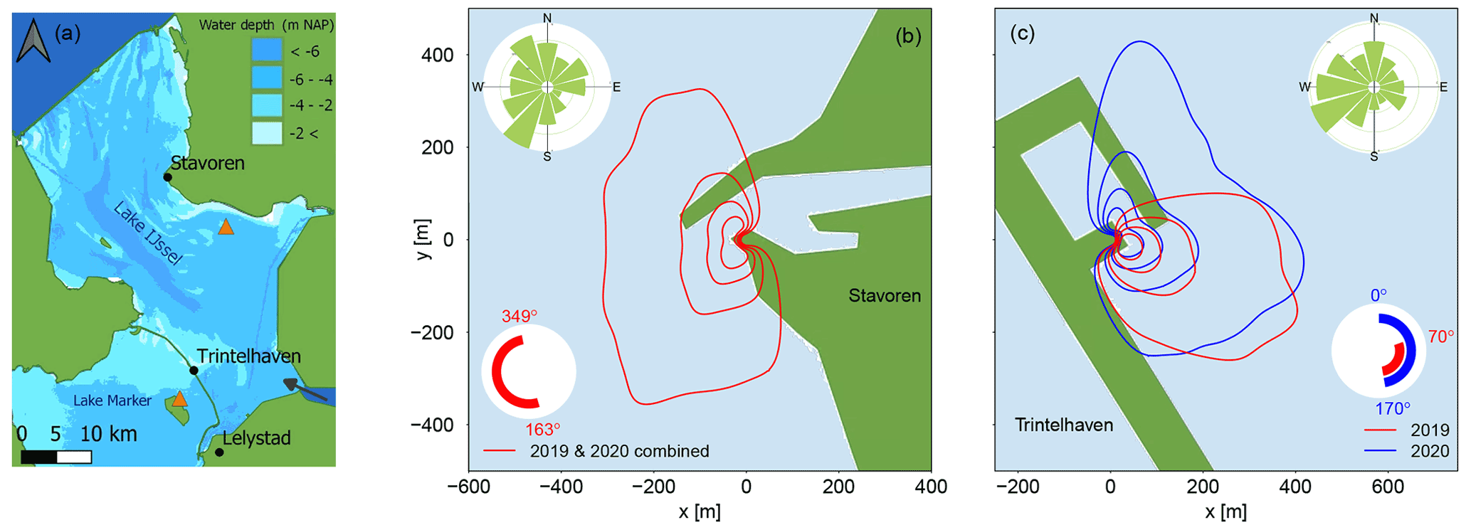
Figure 1Map of the study region and location of the measurement sites. The black dots in panel (a) represent the locations of the turbulent flux observations (Stavoren and Trintelhaven) and the locations where supplementary meteorological data were gathered by the Royal Netherlands Meteorological Institute (Stavoren and Lelystad). The orange triangles are the locations of water temperature measurements performed by the Directorate-General for Public Works and Water Management (Rijkswaterstaat). The black arrow indicates the location where water from the IJssel River enters Lake IJssel. Panels (b) and (c) illustrate the sampling area that is measured by the flux tower for onshore wind conditions, with the contour lines representing 20 %, 40 %, 60 %, and 80 % of the footprint area from inside to outside respectively. This was based on a flux footprint analysis using the model of Kljun et al. (2015). The circular insets at the bottom of both panels indicate the wind directions that are included in the analysis of open water evaporation. At Trintelhaven, shown in panel (c), this angle has shifted from the year 2019 to 2020 following the change in the direction of the eddy covariance instrument (see text). The circular insets at the top of both panels represent the average wind conditions as illustrated by a wind rose.
2.2 Site description, instrumentation, and data
An eddy covariance (EC) measurement system was mounted in a telecommunication tower that is located at the shoreline in the city of Stavoren on the north-east coast of the lake (see Fig. 1a). Its favourable position in relation to the predominant south-westerly wind direction in combination with a pre-existing telecommunication tower renders this location suitable for the measurements needed to analyse the dynamics of open water evaporation. An additional benefit of this location is that it allows a comparison between the dynamics of terrestrial evaporation and open water evaporation by selecting time intervals based on the footprint of the flux tower. An integrated open-path infrared gas analyser and 3D sonic anemometer (IRGASON) instrument (Campbell Scientific) was installed at a height of 7.5 m above the land surface and was pointed towards a heading of 220∘. The IRGASON measures the water vapour and CO2 concentration, air temperature (by the sonic anemometer), barometric pressure, and the three wind components at a sampling frequency of 20 Hz. In addition, air temperature and relative humidity were both measured at 5.9 and 7.4 m height using HMP155A sensors (Campbell Scientific).
In the harbour of Trintelhaven, located in the middle of the Houtribdijk embankment, another telecommunication tower was equipped with the same EC system, installed at a height of 10.8 m above the surface. This location is surrounded by water, with Lake IJssel on the east of the embankment and lake Marker on the west. The IRGASON pointed in a 240∘ direction for the summer period of 2019 and in a 92∘ direction as of January 2020. The latter change maximized the suitable viewing angle of the IRGASON, considering the dominant wind direction and the position of the telecommunication tower and Lake IJssel. HMP155A sensors were used to measure the air temperature and relative humidity at two heights, namely 9.1 and 10.9 m. The measurement height at the two locations (Stavoren and Trintelhaven) differ. In our analysis, we have not adjusted the measurements to an equivalent height. In theory, the small height difference will not affect the heat fluxes under the assumption of a constant turbulent flux layer.
Practical issues precluded observations of the four radiation components and water temperature at the sites. Therefore, observations of global radiation were obtained from the automated weather stations employed by the Royal Netherlands Meteorological Institute (KNMI) in Stavoren and Lelystad. The KNMI weather station in Lelystad is assumed to be representative of Trintelhaven. The sub-skin water temperature, used to estimate the water vapour pressure at the air–water surface, was retrieved from the hourly sub-skin Sea Surface Temperature product with a 0.05∘ spatial resolution derived from the Meteosat-11 satellite. The product specifications describe a target accuracy with a bias of 0.5 ∘C and a standard deviation of 1.0 ∘C. From this product, the grids belonging to the locations of Stavoren (52∘53′06.2′′ N, 5∘21′04.1′′ E) and Trintelhaven (52∘38′03.8′′ N, 5∘25′03.8′′ E) were retrieved. Data were only available during cloudless days. Furthermore, routinely measured water temperatures of Lake IJssel were retrieved from the Directorate-General for Public Works and Water Management (Rijkswaterstaat). For this, the Friese Kust and Marker Wadden stations (orange triangles in Fig. 1a) were used; the water temperature at these stations is measured at a depth of −1.5 m NAP and −1.2 m NAP respectively. Although a strong vertical water temperature gradient typically exists near the water surface, a good correlation (R2=0.71 and R2=0.94 for the summer period of 2019 at Stavoren and Trintelhaven respectively) was found between the sub-skin water temperature from the satellite product and the water temperature measured at the larger depths.
2.3 Data processing
The analysis in this study focuses on the data collected during the summer periods of 2019 and 2020. Latent heat flux (LE) can be calculated using the covariance in vertical wind speed and specific humidity, and sensible heat flux (H) can be calculated using the covariance in vertical wind speed and temperature:
where ρa [kg m−3] is the air density, Lv [J kg−1] is the latent heat of vaporization, cp [J K−1 kg−1] is the specific heat of air at constant pressure, w [m s−1] is the vertical wind speed, q [kg m−3] is the specific humidity, and T [K] is the air temperature.
For this, raw EC data were processed according to Foken et al. (2012). The processing steps were performed using the EddyPro software (EddyPro, 2021). This software package was chosen because it is widely used for processing eddy covariance measurements. The results compare well with the results directly obtained through the incorporated EasyFlux DL software made for the IRGASON (EasyFlux, 2017).
Firstly, the raw data underwent quality control using several criteria in order to remove faulty or corrupt data. This included testing for completeness. If more than 5 % of the expected high-frequency data within the chosen averaging interval were missing, the interval was flagged. Unrealistic values for each variable based on fixed individual thresholds were removed. Spikes were detected and eliminated in accordance with the algorithm of Mauder et al. (2013). Furthermore, according to the approach of Vickers and Mahrt (1997), the data were screened for too many poor-resolution records and for too many so-called “dropouts”, referring to jumps in the data that continue over a longer period and are consequently not recognized as spikes. Density fluctuations were compensated for using the Webb–Pearman–Leuning (WPL) approach (Webb et al., 1980). If the signal strength of the gas analyser fell below 70 %, the data were also removed. Secondly, this quality-checked dataset was further processed to obtain calculated raw fluxes. Next, coordinate rotation of the sonic anemometer using the double-rotation method (Wilczak et al., 2001) was applied to correct for an imperfectly levelled sonic anemometer, and trends were removed using block averaging.
From this point, the final covariances were calculated and were subject to two essential tests, as described by Foken et al. (2004): (i) a test of stationarity during the averaging interval (30 min) and (ii) a test of whether there were well-developed turbulent conditions such as those required for proper usage of the Monin–Obukhov similarity theory. This yielded time series containing raw fluxes. As a final step, spectral corrections were applied to account for high- and low-frequency losses (Massman, 2000; Moncrieff et al., 2004), and the correction developed by Schotanus et al. (1983) was also applied to account for the humidity effect on the sonic temperature, which becomes specifically important for locations near waterbodies. After iterating the last steps and incorporating the quality tests, a fully quality-checked half-hourly flux dataset was obtained. Within this dataset, gaps of a maximum of one data point (i.e. half an hour) were linearly interpolated. Larger gaps were intentionally not gap filled, as this would create too many synthetic results which would interfere with our aim of performing a process-oriented study. Hourly data were obtained by aggregating the half-hourly dataset with no further gap-filling action taken. Daily averages were only calculated from the half-hourly dataset if valid data were available for at least 66 % of the time.
2.4 Flux footprint analysis
The flux footprint is computed to quantify the sampling area that contains the sinks and sources contributing to the measurement point. Additionally, the relative contribution of each upwind location to the measured flux is quantified. In Fig. 1b and c, the contour lines represent 20 %, 40 %, 60 %, and 80 % of the footprint area, where the 20 % line is located closest to the measurement tower. This footprint analysis helps to decide which wind directions to include in the analysis based on the area of interest. The size of the footprint depends on the measurement height, atmospheric stability, and surface roughness (McGloin et al., 2014). In this study, we used the footprint model developed by Kljun et al. (2004) with the Flux Footprint Prediction (FFP) R code (Kljun et al., 2015). For Stavoren, this footprint analysis showed that the flux data for wind directions between 163 and 349∘ are available for analysis of Ewater, whereas the remaining wind directions represent the fetch over land and could, therefore, be used for comparison with terrestrial evaporation. At Trintelhaven, we were only interested in the fetch over Lake IJssel. Therefore, the flux data for Trintelhaven were disregarded for wind directions between 170 and 70∘ for the summer of 2019. After changing the direction of the IRGASON, this yielded a larger angle from which data could be used during the summer of 2020, namely for wind directions between 0 and 170∘. Given the dominant south-westerly wind direction, visualized with a wind rose (inset at the top of Fig. 1b and c), this means that a large part of the data unfortunately had to be rejected at Trintelhaven.
2.5 Regression model
A regression analysis was performed to explore which variable or combination of variables could best explain the dynamics of Ewater. The “leaps” package in R was used to identify the best regression model, and the residual sum of squares was used as a metric to find the best model given the predictors. The variables included in this analysis were wind speed, VPD, global radiation, vertical vapour pressure gradient, and water temperature. These variables are generally considered to be important in describing Ewater and are partially included in the models of Dalton and Penman. To be specific, the choice of including VPD and vertical vapour pressure gradient in the regression analysis was motivated by the apparent drivers of the Dalton and Penman equations. VPD was given preference over air temperature as the dependent variable in the regression analysis due to its explicit mention in the Penman equation, whereas air temperature only features implicitly in the definition of the slope of the vapour pressure gradient (s) and in the definition of VPD. From the regression analysis, a data-driven model was developed to estimate Ewater of Lake IJssel. This was done for both locations, Stavoren and Trintelhaven. For each individual variable, as well as for all combinations of variables, both the sum and product, a regression model was created. In the regression analysis, simple linear regression models (Eq. 3), multiple linear regression models (Eq. 4), and quadratic regression models (Eq. 5) were considered. The equations of these models are prescribed as follows:
where Y is the dependent variable, Xi is the explanatory variable(s), β0 is the intercept, βi is the parameter(s), and ϵ is the error term. The explanatory variable(s) Xi was prescribed to be either a single variable or the product of multiple variables, except in Eq. (4), where Xi can only be a single variable. Statistical significance (p<0.05) was tested. From the multitude of regression models that resulted from the regression analysis, the best model was chosen by using the adjusted R2 and RMSE metrics to evaluate the fit of each regression model. We aimed to find the best model; however, we were also interested in finding the best simple model that used a maximum of two variables while still being able to explain the dynamics of Ewater well. The summer season of 2019, here taken as 1 May to 31 August, was used as the training dataset to calibrate the data-driven model, and the dataset of the summer of 2020 was used for validation. The analysis was performed at hourly and daily timescales.
The above-mentioned procedure was repeated using only routinely measured observations. This was done to explore the possibility of using routine observations to make accurate estimations of Ewater, instead of continuing the labour-intensive and expensive measurements with the eddy covariance systems. As described previously (see Sect. 2.2), data from automatic meteorological stations of the KNMI were used to obtain global radiation measurements and were complemented by air temperature, wind speed, and relative humidity, which are routinely measured at these stations. There are no available routine observations of the skin water temperature of the lake. As an alternative, the use of water temperature data routinely measured by Rijkswaterstaat at depths ranging from 1.2 to 1.5 m was explored.
The resulting regression model was compared to the models of Dalton, Penman, and Makkink (see Eqs. 6, 8, and 12) to give an indication of the (dis)agreement of the variables involved in explaining the dynamics of Ewater and its form. Dalton's model is based on the empirical relationship that was found between evaporation and the product of a wind function and the vertical vapour pressure difference, which can be written as follows:
Here, e2 [kPa] is the vapour pressure at 2 m height, es(T0) [kPa] is the saturation vapour pressure at the surface, and f(u) [W m−2 kPa−1] is the wind function which takes the following form (Penman, 1956; De Bruin, 1979):
where u2 [m s−1] is the wind speed at 2 m height. Although the representation of the Dalton models may seem simple, obtaining reliable measurements of surface temperature is challenging.
Similarly, Penman's equation, which is derived from Dalton's equation, can be written as follows:
where s [kPa ∘C−1] is the slope of the saturated vapour pressure curve at air temperature; γ [kPa ∘C−1] is the psychrometric constant; es(T2)−e2 [kPa] is the vapour pressure deficit (VPD) at 2 m height; and Q* [W m−2] is the available energy at the surface, which can be defined as Rn−G, where Rn [W m−2] is net radiation, and G [W m−2] is the downward heat flux from the water surface. Net long-wave radiation was calculated following Eqs. (2.24) and (2.28) from Moene and van Dam (2014):
where Lin [W m−2] is the incoming long-wave radiation, Lout [W m−2] is the outgoing long-wave radiation, ϵa [–] is the apparent emissivity that is a function of the fraction of cloud cover, σ [ W m−2 K−4] is the Stefan–Boltzmann constant, Ta [K] is the air temperature, Le,out [W m−2] is the emitted long-wave radiation, and ϵs is the surface emissivity. Net short-wave radiation was calculated as follows (Allen et al., 1998):
where K* [W m−2] is the net short-wave radiation, Kin [W m−2] is the global radiation, and α [–] is the albedo values for which monthly values were calculated as a function of latitude (Cogley, 1979).
Priestley and Taylor (1972) found that the aerodynamic term of Penman's equation is approximately one-fourth of the radiation term. Makkink (1957) found that this equation could be simplified even more for estimating daily evapotranspiration from well-watered surfaces. Under these conditions, G is assumed to be negligible, and a constant ratio between net radiation and global radiation of on average 0.5 can be assumed, which results in the following equation (Makkink, 1957):
According to Penman's derivation, G is assumed to be negligible for timescales of a day to several days for shallow water surfaces, similar to land surfaces, and the term is often ignored because of the difficulty involved with measuring it. However, for waterbodies that are several metres deep, the impact of neglecting G on the energy balance can be considerable (Keijman, 1974; de Bruin, 1982; Tanny et al., 2008; van Emmerik et al., 2013). For these waterbodies, G should be considered as a result of temperature changes integrated over the volume of the water column, in contrast to a land surface where the impact of G is more superficial. It should be clearly noted that, although Lake IJssel is a lake that is several metres deep, we have neglected G in the following analyses for the following two reasons: (1) we were not able to measure it, and (2) we wished to adhere to how Penman's equation is typically employed for shallow water surfaces.
3.1 Data quality and quantity
To guarantee the data quality of the flux measurements, quality checks were performed, as described in Sect. 2.3. After the quality control, 66 % and 64 % of the latent heat flux data were available in 2019 for Stavoren and Trintelhaven respectively. In 2020, this number was lower: 49 % and 59 % for Stavoren and Trintelhaven respectively. Part of the available quality-checked data needed to be rejected based on the flux footprint analysis. This led to a further reduced number of available data for 2019: 42 % and 13 % of the total data for Stavoren and Trintelhaven respectively. In 2020, the total available latent heat flux data was 33 % and 19 % for Stavoren and Trintelhaven respectively. The reduction of the available data at Trintelhaven was larger given the combination of dominant south-westerly winds and the location of the instrument at the south-west border of Lake IJssel (see Fig. 1a). The number of total available flux data is at the lower end (although not unusual) of the data availability reported in other studies on lakes, which is typically in the range of 16 %–59 % (Vesala et al., 2006; Nordbo et al., 2011; Bouin et al., 2012; Mammarella et al., 2015; Metzger et al., 2018).
No clustering was found in the availability of latent heat flux data during daylight hours (06:00–21:00 LT) compared to the night (21:00–06:00 LT). In the final half-hourly dataset, latent heat flux data were available during 56 % of the total half-hour daytime periods in Stavoren in the summer of 2019 and during 49 % of the periods during night-time. In the summer of 2020, this was 49 % and 40 % for daytime and night-time respectively. For Trintelhaven, the corresponding fractions were 10 % and 18 % during daytime and night-time in the summer of 2019 respectively. The difference between the daytime and night-time fractions was smaller during the summer of 2020, with 18 % and 21 % of data available respectively.
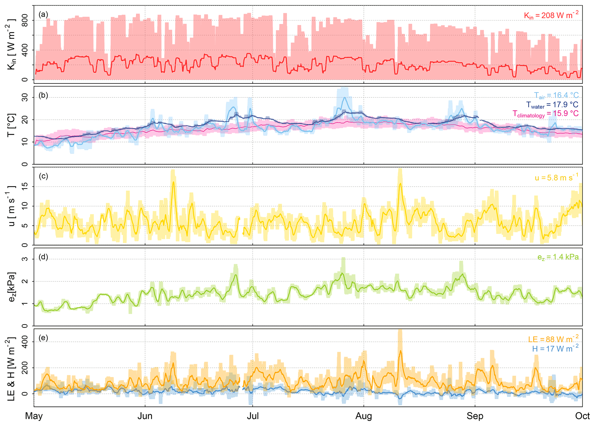
Figure 2Meteorological conditions in Stavoren in 2019, showing running daily means of global radiation (a), air temperature (current and climatology) and water temperature (b), wind speed (c), vapour pressure (d), and turbulent fluxes (e). The shaded area represents the range between the minimum and maximum observed values, and the numbers reported in the top right of each panel provide the average values of the respective variables during the presented months.
3.2 Meteorological conditions
Similar dynamics were observed at both locations (Stavoren and Trintelhaven). Here, we only show the meteorological conditions observed in Stavoren during the period from 1 May to 30 September 2019 (Fig. 2; see Appendix A for the meteorological conditions in Stavoren in the summer period of 2020). Figure 2 illustrates the dynamics and trends of the meteorological variables and the heat fluxes before, during, and after the summer period, and it explores if any visible lags, for instance, would occur at this timescale. Table 1 provides an indication of the source of the data for the variables that will be elaborated on in this section. According to the measurements of the KNMI, both measurement stations received on average the same amount of global radiation for the period from 1 May to 30 September 2019, namely 208 W m−2 in Stavoren and 204 W m−2 at Lelystad, with the latter assumed to be representative of Trintelhaven. The average air temperature that we measured with the HMP155A sensor is lower in Stavoren (16.4 ∘C) than in Trintelhaven (18.0 ∘C). These temperatures are higher than the climatological mean observed by the KNMI (period 1991–2020) for the same months: 15.9 ∘C in Stavoren and 16.1 ∘C at Lelystad (KNMI, 2021a). The water temperature measured by Rijkswaterstaat in the vicinity of Stavoren was on average 17.9 ∘C, and the water temperature at Marker Wadden close to Trintelhaven was on average 18.3 ∘C. The time series of water temperature shows a more smooth, attenuated, and lagged signal compared with the air temperature. At both measurement locations, the measured wind speed observed with the IRGASON is similar, with an average wind speed of 5.8 m s−1 in Stavoren and 5.6 m s−1 at Trintelhaven, without a distinct seasonal pattern. The vapour pressure that we measured follows the seasonal cycle of the air temperature and has a mean value of 1.4 kPa in Stavoren and 1.6 kPa at Trintelhaven. Figure 2e shows the observed turbulent fluxes. The sensible heat flux remains consistently low throughout the summer period, with an average value of 17 W m−2 in Stavoren and 25 W m−2 at Trintelhaven. The latent heat flux is more than 4 times as high on average, with mean values of 88 W m−2 in Stavoren and 91 W m−2 in Trintelhaven. Basic statistics on the observed latent heat flux can be found in Appendix B. The latent heat flux displays trends similar to those for the measured wind speed, indicating that the two variables are correlated (R2=0.61). Based on the average rates of sensible and latent heat flux, the Bowen ratio is 0.19 in Stavoren and 0.27 at Trintelhaven.
Table 1Sources of data used in this study. The variables measured at our locations in Stavoren at 7.5 m and in Trintelhaven at 10.8 m were sampled at high frequency (20 Hz) and aggregated to hourly data. The data retrieved from KNMI stations in Stavoren and Lelystad are provided at hourly timescales and were measured at 1.5 m height above the land surface, and 10 min water temperature data measured by Rijkswaterstaat at Friese Kust at −1.5 m NAP and Marker Wadden at −1.2 m NAP were aggregated to hourly timescales.
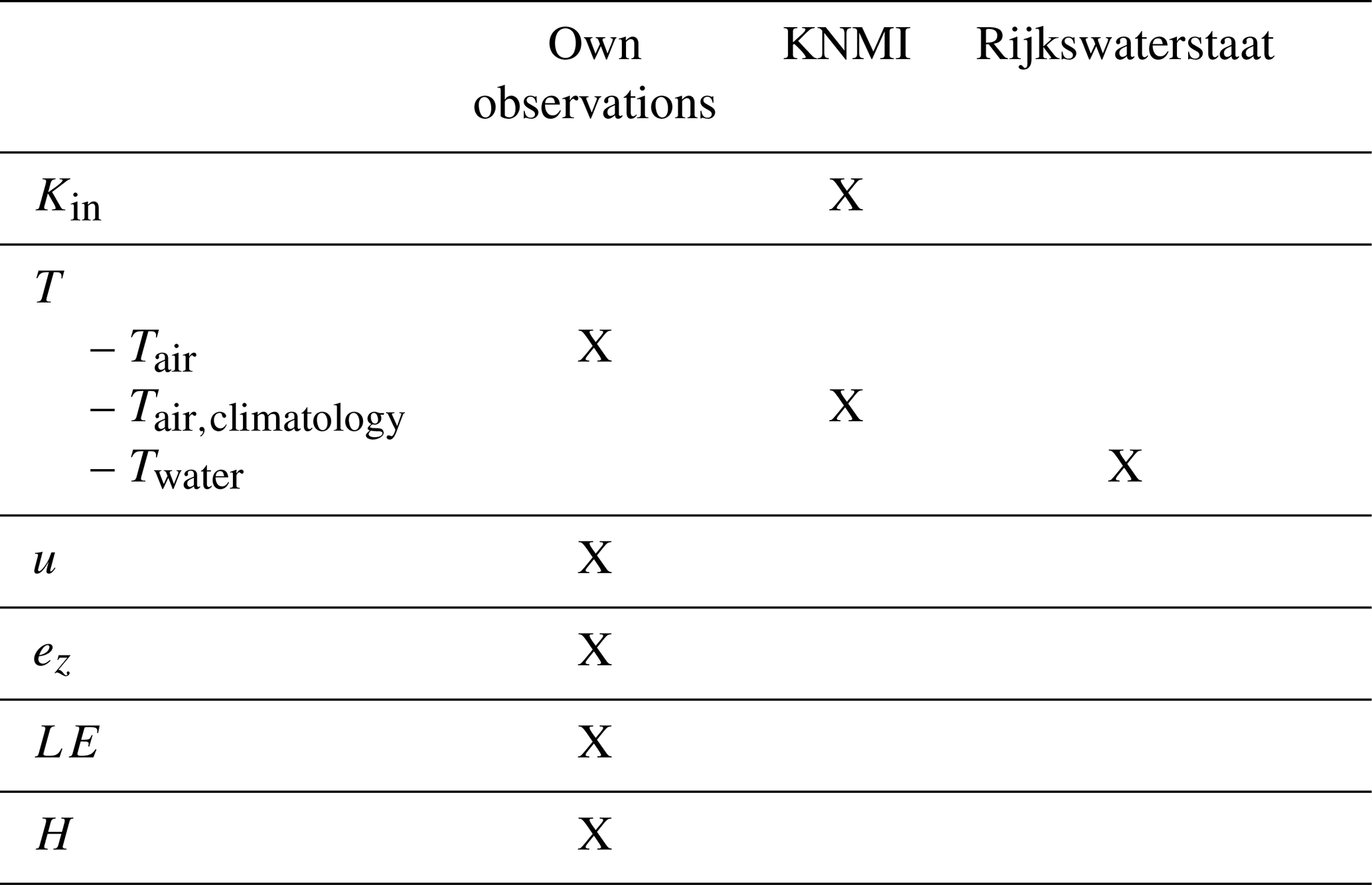
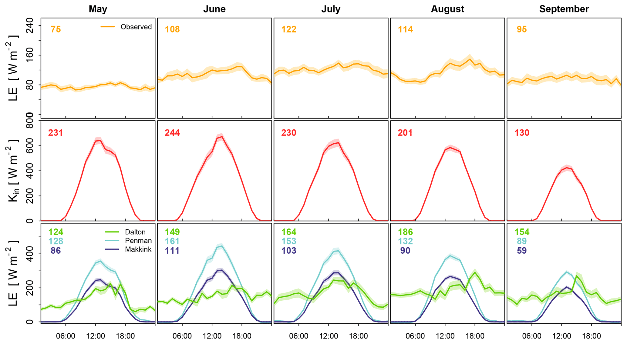
Figure 3An illustration of the decoupling in Stavoren in 2019 between the monthly average diurnal cycles of observed latent heat flux (top panels) and global radiation (middle panels), with the latter forming the basis of the frequently used evaporation models of Penman (1948) and Makkink (1957). These models are shown together with the model of Dalton (1802) in the bottom panels. Note that some variables included in the evaporation models are measured at heights above the 2 m that is prescribed (see Eqs. 6–12). Additionally, all three models are generally used on a daily basis, but they are presented here to show the underlying daily cycle. The shaded area represents the uncertainty, which is defined as the standard deviation divided by the square root of the number of observations. Average daily means of the respective variables are indicated by the number in the top left of each panel and display the average course over the summer period.
3.3 Diurnal and intra-seasonal variability in latent heat flux
The monthly average diurnal variability in observed LE, based on hourly data, is shown in the top panels of Fig. 3 for Stavoren for the same period as in Fig. 2 (i.e. 1 May–30 September 2019). The diurnal variability in LE does not have a strong diurnal cycle; rather, it is constant throughout the day and night, which is in contrast to terrestrial evaporation that typically peaks during the day. However, in August, the LE signal shows a distinct peak during the late afternoon and lower values during the night and early morning. The highest average diurnal LE is reached in July, as indicated by the number in the top left-hand corner of each panel in Fig. 3. Global radiation measured at the KNMI meteorological stations in Stavoren is shown in the middle panels. A clear distinctive diurnal cycle is visible with a peak in the afternoon, and the highest average value is found in June at both locations. The global radiation has served as input for the commonly used radiation-based models of Penman (1948) and Makkink (1957), of which the average diurnal cycles are shown in the lower panels of the same figures. Recall that G was omitted in Penman's model in this analysis (see Sect. 2.5). The diurnal cycles of the models of Penman and Makkink closely follow the pattern of the global radiation but with a lower amplitude. The highest average LE values are found in June for these models, in contrast to observed LE which is found to be highest a month later. In the lower panels, the average diurnal cycle of LE that follows from Dalton's model is shown as well. There is no strong diurnal cycle visible, similar to the observed LE, but rates are generally highest during daytime. The highest average LE values are found in August. The observed monthly average diurnal dynamics were found to be similar in Trintelhaven (see Appendix C).
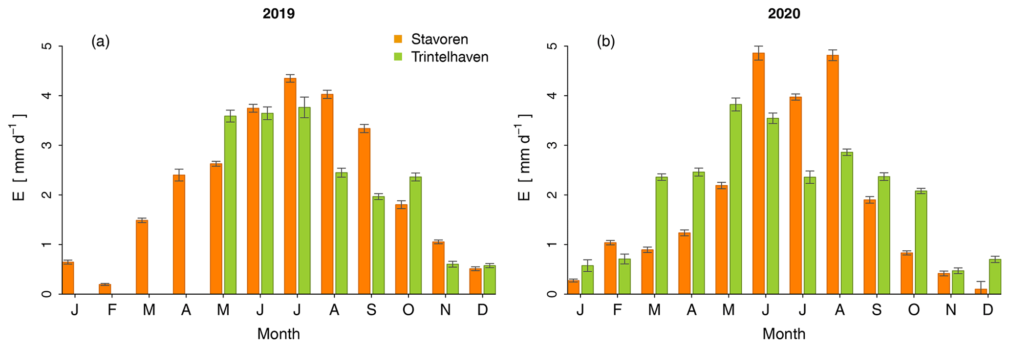
Figure 4Yearly cycle of observed open water evaporation in Stavoren (orange) and Trintelhaven (green) based on half-hourly data for both of the respective years, 2019 and 2020. The bars indicate the monthly average evaporation, and the whiskers represent the uncertainty, which is defined as the standard deviation divided by the square root of the number of observations.
The extension of the time series to a complete year in order to visualize the seasonal variability shows a clear seasonal cycle that is reminiscent of the influence of a radiation component on Ewater (Fig. 4). The bars represent the monthly average Ewater rate based on half-hourly data. For the year 2019, the evaporation rate is highest in July for both locations: 4.3 mm d−1 in Stavoren and 3.8 mm d−1 in Trintelhaven. The lowest values are 0.2 mm d−1 in Stavoren (February) and 0.6 mm d−1 in Trintelhaven (December); note that data from January–February 2019 are lacking for the latter location. In 2020, similar rates are found in winter, 0.1 mm d−1 in Stavoren (December) and 0.5 mm d−1 in Trintelhaven (November), while the summer of 2020 now has a dip in July instead of being the peak.
3.4 Drivers of open water evaporation
Based on historical theory, it is known that governing factors of Ewater include the gradient of vapour pressure above the water surface and some measure of the strength of the turbulence (Dalton, 1802; Penman, 1948; De Bruin, 1979; Brutsaert, 1982). These variables form the ingredients of the so-called “aerodynamic method” or “mass transfer approach” (Brutsaert, 1982). Here, we tested which variable or combination of variables can best explain the dynamics of observed Ewater at Lake IJssel at both an hourly and daily temporal resolution. The variables included in this analysis are global radiation, vertical gradient of vapour pressure, vapour pressure deficit, sub-skin water temperature, and wind speed. Recall that air temperature was not explicitly included in the regression analysis, as explained in Sect. 2.5. We expect that including air temperature as a separate dependent variable might have explained a part of the evaporation dynamics, as air temperature affects surface temperature through the sensible heat flux. The surface temperature, in turn, affects the vapour pressure gradient and, thus, evaporation. However, due to the large thermal buffer of a waterbody, we expect that there is a less direct coupling between the sensible heat flux and the latent heat flux at short timescales.
The proportion of the dynamics of Ewater that can be explained by the variable or combination of variables is shown in Venn diagrams, with the adjusted coefficient of determination (R2) written inside (see Fig. 5). The higher the adjusted R2, the bluer the colour in the figure. Adding a variable will not always result in a higher adjusted R2 value, as the adjusted R2 takes the degrees of freedom into account; therefore, if an added variable only slightly correlates with the dependent variable, it can lead to a decrease in the adjusted R2 value. Values of the adjusted R2 were removed if the model fit was found to be insignificant (p<0.05). Venn diagrams a and c on the left-hand side of Fig. 5 illustrate the analysis based on hourly data, and diagrams b and d on the right-hand side of Fig. 5 are based on daily data. The outer “leaves” of the diagram represent the single variables, whereas combinations of variables are taken into account towards the centre of the diagram in order to explain the dynamics of Ewater. Both the sums and the products of the combined variables are analysed (Fig. 5 and Appendix D respectively). Based on these diagrams, a decision was made regarding which variables to include in the data-driven model to estimate Ewater. The prominent blue colour connected to wind speed already tells us that this is an important variable to include, which is in agreement with Dalton's model and was also visible from Fig. 2 (R2=0.61). Global radiation has the lowest adjusted coefficient of determination, which agrees with our findings in Figs. 2 and 3.
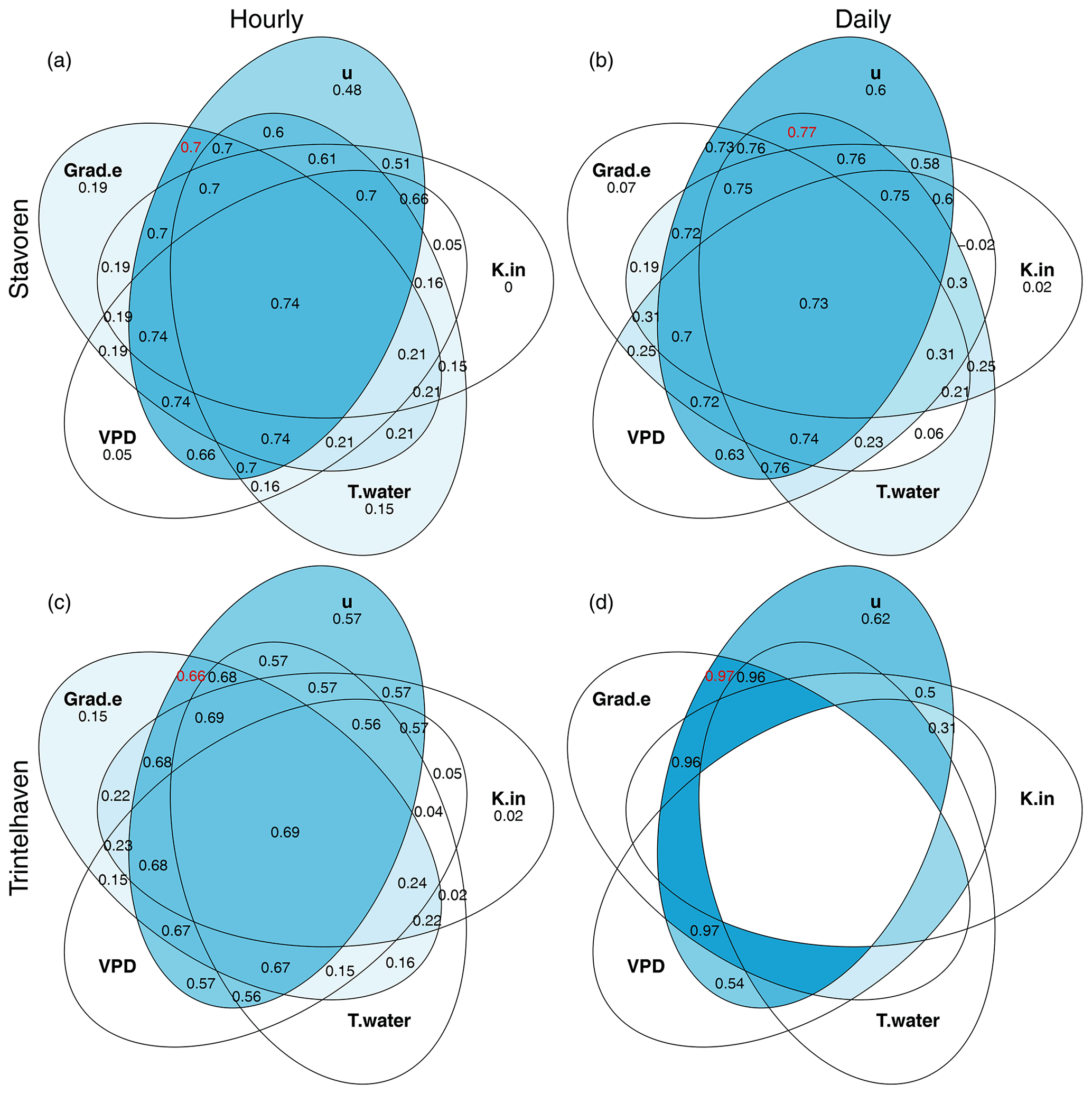
Figure 5A systematic exploration of which variable or combination of variables (sums) can best explain the dynamics of open water evaporation. The outer “leaves” of the Venn diagram represent the model fit based on the single variables, whereas the summed combinations of variables are represented towards the centre of the diagram. Within each leaf, the adjusted R2 value is depicted. The higher this value, the bluer the colour of the leaf. The red number indicates the highest R2 value, indicating the best combination found for a maximum of two variables, i.e. the best “simple” model. The R2 values were removed if the model fit was found to be insignificant (p<0.05). The analysis is based on data from the summer of 2019 and is performed at an hourly timescale – Stavoren (a) and Trintelhaven (c) – and a daily timescale – Stavoren (b) and Trintelhaven (d).
3.4.1 Calibration
For both locations, two models were developed: (i) a model that included the variable or variables that explain most of the variability in Ewater (and, thus, had the highest adjusted R2), and (ii) a model that only used one or two variables that were still able to explain a significant portion of the variability in Ewater (the number depicted in red in the Venn diagrams in Figs. 5 and D1). At the hourly timescale, the best model fit, indicated by the highest R2 value, is reached when the sum of (almost) all five variables are included (R2=0.74 and R2=0.69 at Stavoren and Trintelhaven respectively). Moving from the outer leaves towards the centre of the diagram, we find that the most simple hourly model that still explains a large portion of the variance (i.e. the red numbers) includes only wind speed and the vertical gradient of vapour pressure: R2=0.70 in Stavoren (Fig. 5) and R2=0.69 in Trintelhaven (Fig. D1). This is in agreement with Dalton's model. At the daily timescale in Stavoren, we see a shift in the variables that are included in the “simple” model. The sum of wind speed and water temperature reaches the highest R2 value (R2=0.77). Unfortunately, very few data points (N=10) were left at the daily timescale at Trintelhaven, which led to many insignificant model fits (values were removed from those intersecting areas). However, a couple of models were found to be significant, and the sum of wind speed and the vertical gradient of vapour pressure again showed the highest R2 value (R2=0.97). The relatively high adjusted R2 values of these simple model fits, compared with models including more than two variables, indicate that the added value of using more than two variables is virtually nil. The results from the Venn diagrams form the base to create the data-driven models for which the data collected in 2019 are used. Both linear and quadratic regression models were considered, as explained in Sect. 2.5.
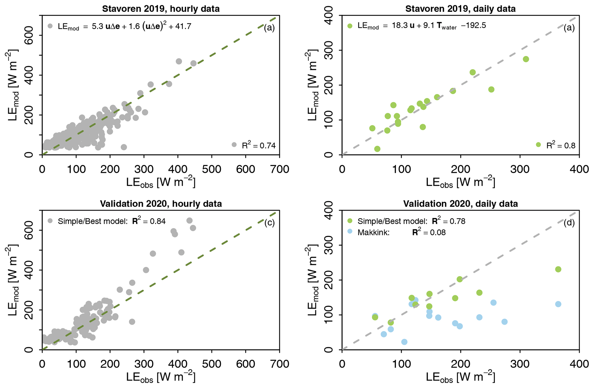
Figure 6Evaluation of the developed “simple” and “best” data-driven models based on our own observations during the summer of 2019 (calibration) and 2020 (validation) to estimate open water evaporation in Stavoren at hourly (a) and daily (b) timescales. The model equations are shown in panels (a) and (b) and differ from the models found based on routinely measured observations (see Table 2a). The results of the validation of the models are presented in panels (c) and (d) for hourly and daily timescales respectively. The simple model was also found to be the best model. The results of estimated evaporation using Makkink's model (light blue) are added to the validation plots as a reference. Model performance is indicated by the values of the coefficient of determination (R2) shown in each panel.
The results presented in the Venn diagrams are used to formulate the regression models. Both the “simple” and “best” fitted model were evaluated, based on hourly and daily data, and are presented in panels a and b of Fig. 6 (Stavoren) and Fig. 7 (Trintelhaven). At both locations, the simple models were also found to be the best models. For both locations, the regression analysis based on hourly data showed that the combination of wind speed and vertical gradient of vapour pressure explains most of the variability in Ewater, leading to R2 values of 0.74 and 0.70 at Stavoren and Trintelhaven respectively. The sum of wind speed and the vertical gradient of vapour pressure was the most important ingredient to explain Ewater at a daily timescale at Trintelhaven (R2=0.98). In Stavoren, the sum of wind speed and water temperature resulted in an R2 value of 0.8. Without predetermination of the variables, we found the same ingredients as used in the Dalton model to be the most important drivers of Ewater at hourly timescales. To determine if the coefficients that were found for the hourly regression models of the two measurements locations differ significantly, an ANOVA (analysis of variance) statistical test was performed (see Appendix E). This analysis showed that the inclusion of the measurement site matters (p<0.05). Therefore, we cannot rule out that the sites are different.
3.4.2 Validation
The models are validated using the data collected in 2020, and the results are presented in panels c and d of Figs. 6 and 7. The adequate R2 values in the validation give confidence in the performance of the models. Validation of the hourly regression model in Stavoren has a higher R2 value (R2=0.84) compared with the calibration period (R2=0.74). In an attempt to explain why a higher R2 value occurs during the validation of the model, we swapped the calibration (now summer of 2020) and validation (summer of 2019) periods. The coefficients of the regression model were recalculated. The R2 value of the validation was now found to be smaller than during the calibration. This provides an indication that the difference in R2 values during calibration and validation seems to be related to the conditions during the two distinct summer periods, and it gives confidence that the model performs well. In addition to the data-driven models, the estimated daily evaporation rates using Makkink's model are plotted for reference, as this model is currently used in the operational water management of Lake IJssel. Makkink's model fails to explain the dynamics of Ewater at a daily temporal resolution, with R2 values near zero.
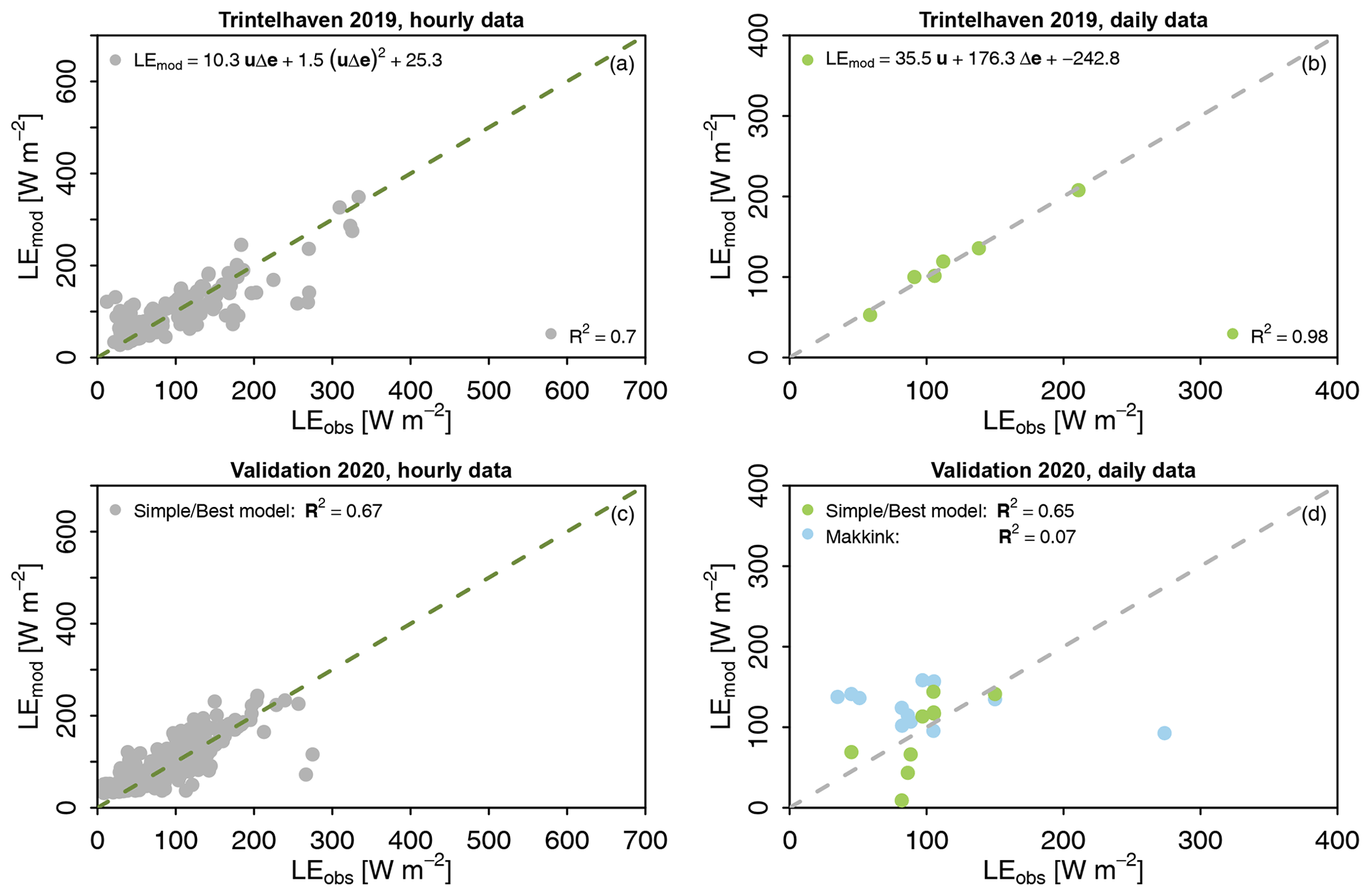
Figure 7Evaluation of the developed “simple” and “best” data-driven models based on our own observations during the summer of 2019 (calibration) and 2020 (validation) to estimate open water evaporation in Trintelhaven at hourly (a) and daily (b) timescales. The simple model was found to be the best model and is shown using light coloured dots. The model equations are shown in panels (a) and (b) and differ from the models found based on routinely measured observations (see Table 2b). The results of the validation of the models are presented in panels (c) and (d) for hourly and daily timescales respectively. The results of estimated evaporation using Makkink's model (light blue) are added to the validation plots as a reference. Model performance is indicated by the values of the coefficient of determination (R2) shown in each panel.
3.4.3 Models based on routinely measured variables
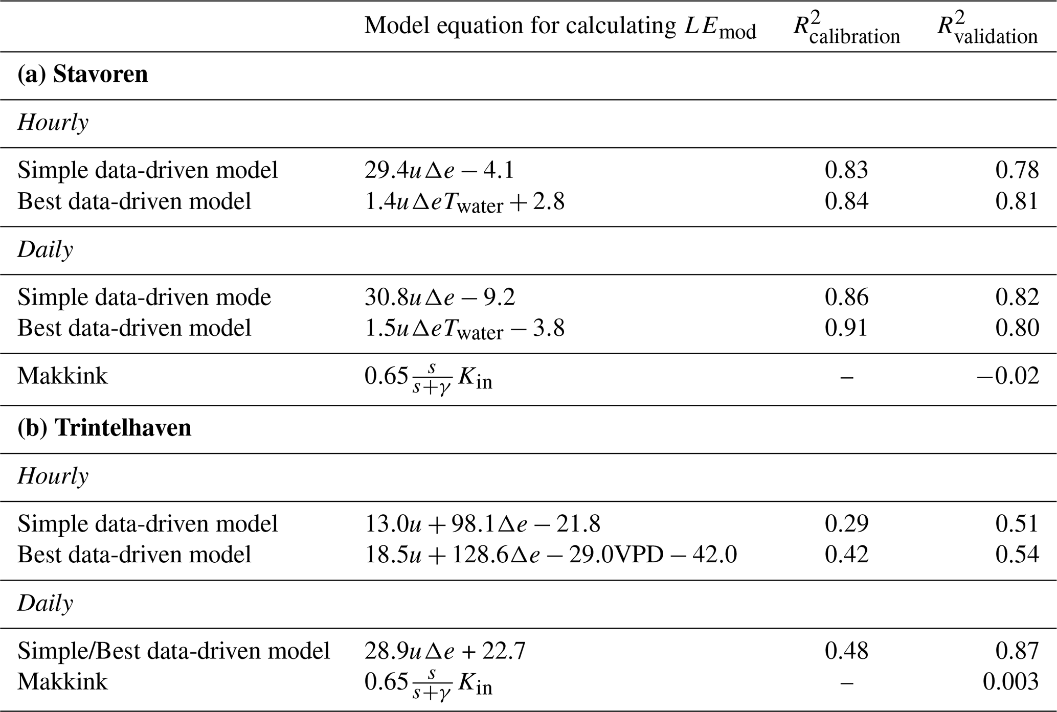
The analysis described above was repeated using only routinely measured observations of meteorological variables at 2 m height by KNMI and observations of water temperatures by Rijkswaterstaat (Table 2a and b). This was done to explore the possibility of using these routine measurement to estimate Ewater, instead of using the expensive and labour-intensive eddy covariance instruments. The regression models found using these routine observations are, especially for Stavoren, able to explain the dynamics of Ewater quite well, and wind speed and the vertical gradient of vapour pressure were the main ingredients for the simple model (R2=0.83 using hourly data and R2=0.86 using daily data). Validation using data from summer 2020 also yields satisfactory results, with high R2 values of 0.78 and 0.82 for hourly and daily data respectively. The results of the simple model for Trintelhaven fall short compared with Stavoren, with R2 values of 0.29 and 0.48 for hourly and daily data respectively. An explanation for this may be that the location of the routine observations is situated further from the target location (Trintelhaven) compared with the observation location for Stavoren (Fig. 1a). At Trintelhaven, R2 values during the validation period are again found to be higher than during the calibration period, which seem to be related to the different conditions during the two summers.
Table 2Evaluation of the developed “simple” and “best” data-driven models based on routinely measured observations (see Sect. 3.4) during the summer of 2019 (calibration) and 2020 (validation) to estimate open water evaporation in Stavoren (Table 2a) and Trintelhaven (Table 2b) at hourly and daily timescales. The models presented here are independent of the results found based on our own observations. The results of estimated evaporation using Makkink's model are provided as a reference. Model performance is indicated by the values of the coefficient of determination (R2).
Our results have shown that the diurnal cycle of observed Ewater shows a distinctively different pattern compared with evaporation estimated using the evaporation models of Penman (1948) and Makkink (1957). Recall that we omitted G in Penman's model in this study. The estimated evaporation using the models of Penman and Makkink better resembles the cycle that was observed at our station in Stavoren when we selected wind directions coming from the land surface, i.e. representing terrestrial evaporation (see Fig. 8). In contrast to the observed terrestrial evaporation, the observed Ewater is not directly coupled to global radiation at these timescales, which is demonstrated by the difference in diurnal variability between global radiation and observed LE (middle and upper panels of Fig. 3). Note that the relation between Ewater and other components of the radiation budget could not be studied because of the lack of observations of these components. In combination with a lack of data on G, this prevented us from fully capturing the role of net radiation in the energy balance of the lake and, thus, in the warming and cooling of the lake, which relates to evaporation through the water surface temperature. Better agreement with the observed diurnal cycle was found for Dalton's model, which is more constant throughout the day. Nevertheless, to date, Makkink's model has been used as a base for calculating Ewater at Lake IJssel (Jansen and Teuling, 2020). We have shown that Makkink's model is not able to explain the dynamics of Ewater for the summer period at the daily timescale. Such a radiation-based approach (including a potential linear correction factor) might lead to the correct daily or monthly evaporation sums, but it will be for the wrong reason.
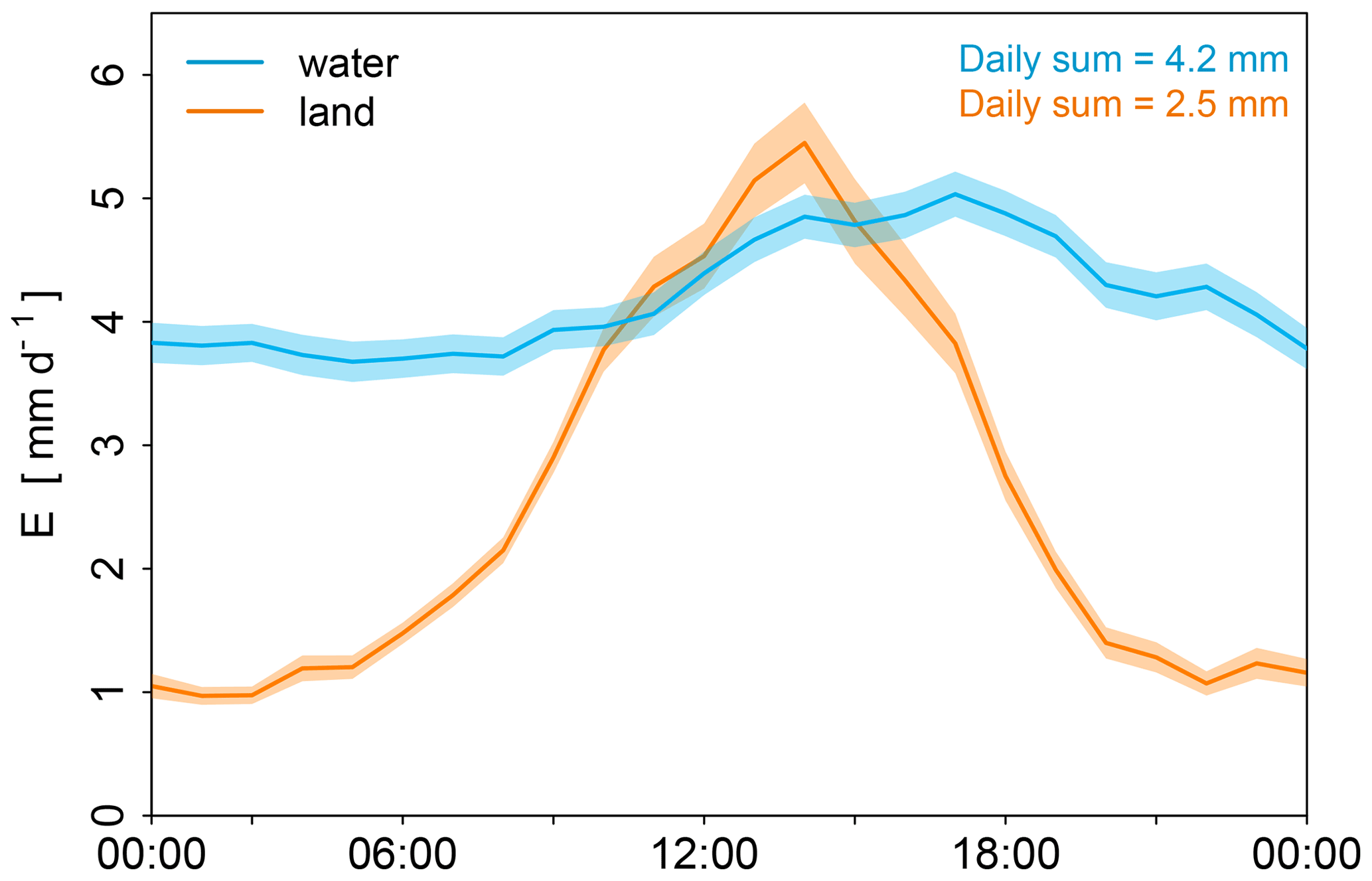
Figure 8Comparison of the average diurnal cycle of open water evaporation (blue) and terrestrial evaporation (orange) observed during the summer period 2019 in Stavoren. The shaded area represents the uncertainty band, which is defined as the standard deviation divided by the square root of the number of observations.
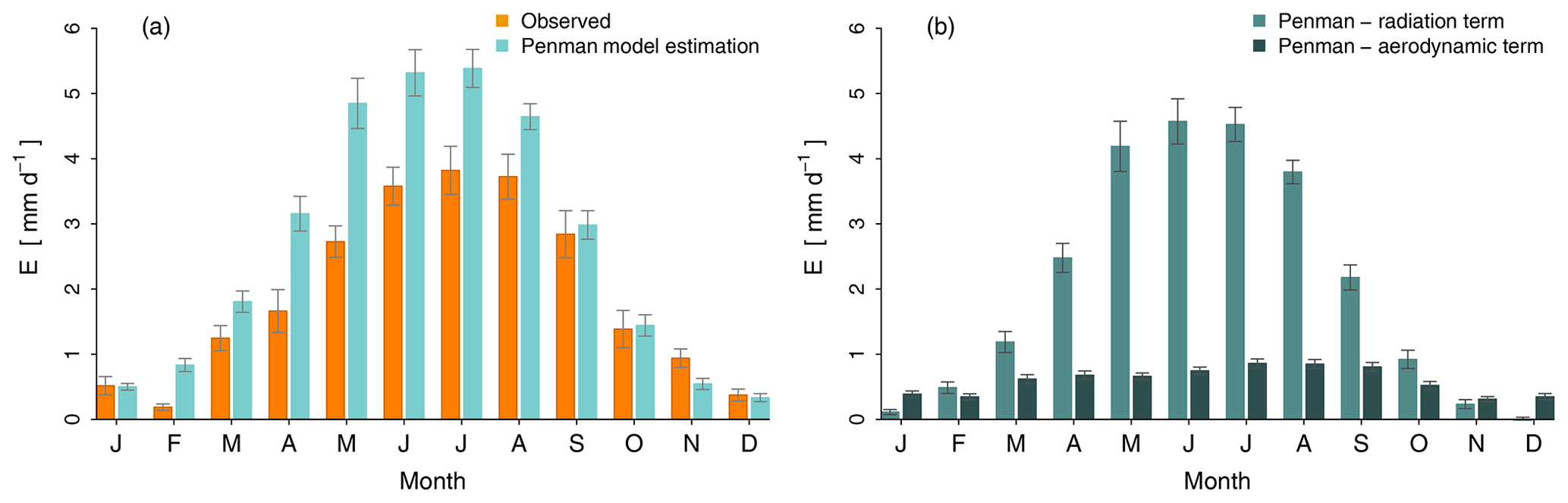
Figure 9Comparison of the annual cycle of observed open water evaporation in Stavoren (orange) and estimated evaporation (blue) using Penman's model (a) based on daily data in 2019. The individual terms of Penman's model are displayed in panel (b), which shows the similarity of the annual cycle between observed open water evaporation and the radiation term of Penman's model. The bars indicate the monthly average evaporation, and the whiskers represent the uncertainty, which is defined as the standard deviation divided by the square root of the number of observations.
From the data-driven modelling that was performed, we found that not radiation but a combination of wind speed and vapour pressure gradient is the most important ingredient to explain the variance in Ewater at short timescales. This is similar to what has been found by studies such as Blanken et al. (2011) and McGloin et al. (2014). It was also noticed that intraseasonal variations in Ewater can be linked to synoptic weather variations through these variables (Lenters et al., 2005; MacIntyre et al., 2009; Liu et al., 2011; Woolway et al., 2020). The same ingredients, wind speed and the vapour pressure gradient, were used in the model by Dalton (1802). By combining and rearranging Eqs. (6) and (7), we can write Dalton's model in the following form:
where Δe [kPa] is es(T0)−e2 [kPa]. This highlights the similarity of the functional form of Dalton's model and our data-driven model that resulted from the regression analysis (see Figs. 6 and 7). When the exact functional form of Eq. (13), i.e. , is fitted to our hourly observations of 2019, we find that coefficients a and b differ (not shown here). This difference is likely related to the height at which our measurements were done (10.8 and 7.5 m above the surface in Stavoren and Trintelhaven respectively) compared with the standard height of 2 m. We found that Penman's model seemed unsuitable for estimating Ewater over the summer period in the form in which we have employed it (i.e. with G omitted). However, when we extended the time series from only the summer period to the whole year, a clear yearly cycle was visible, with a peak in summer that is similar to the cycle of (available) radiation and, thus, to estimates of evaporation using Penman's model (see Fig. 9a). The benefit of Penman's model in this case is that it can easily be decomposed into an aerodynamic term and a radiation term. The individual terms are presented in Fig. 9b. Here, a clear distinction between the yearly cycle of the two Penman terms is visible: the radiation term has a distinct cycle with a peak in June, whereas the aerodynamic term is more constant over the year. This resembles the constancy of observed Ewater found in the diurnal cycle (see Fig. 3).
Another phenomenon that could affect the yearly cycle of evaporation is lake water stability and, thus, mixing depth within the lake. Seasonal changes in lake water stability affect the surface temperature and, therefore, evaporation rates via the vapour pressure gradient. Evaporation, in turn, has a cooling effect on the surface temperature, which increases potential mixing. Supported by a preliminary study where mixing depths were simulated using the FLake model (Voskamp, 2018), we assume that Lake IJssel is fully mixed 70 % of the time. This number is not surprising given the fact that evaporation continues during night-time and with wind speeds that are on average 5.8 m s−1. In addition, the inflow of the IJssel River into the lake is also likely to support mixing. During summer, it is more likely that stable conditions occur, and we cannot directly assume fully mixed conditions. However, we considered a full analysis of this phenomenon to be beyond the scope of the current study.
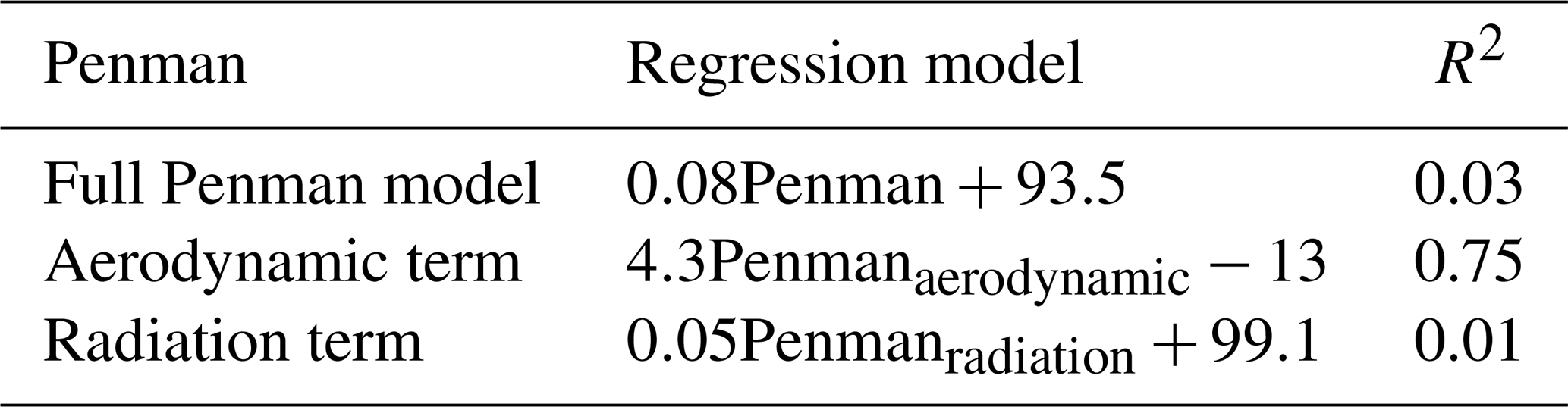
Linking back to the shorter time series spanning the summer months of 1 May to 31 August, we can see that a simple linear relationship exists between observed Ewater and the aerodynamic term of Penman's model. In contrast, the variability in radiation is uncorrelated with observed Ewater (see Table 3). The high correlation between the aerodynamic term of Penman, which includes similar variables to Dalton's model, and observed Ewater strengthens the finding that our data-driven model is embedded into the well-known theory. We are aware that using a statistical modelling approach has its limitations, as it does not account for the actual physical processes in the way that they might be included in physically based models such as FLake (Mironov, 2008) for modelling lake evaporation. However, in such physically based models, empirical relations are also included (e.g. the wind function in Dalton's and Penman's model), and parameters need to be statistically estimated. Furthermore, if drivers of open water evaporation appear to be a function of the temporal resolution, it should be concluded that models, including physical models, can only be properly used at the right temporal resolution. Considering this, we think that statistical modelling is a clean and simple approach that can provide a direct indication of (and insight into) the most relevant input parameters involved in explaining the variation in evaporation, without making a priori assumptions regarding the processes or relations that might be relevant. Therefore, we argue that our model is robust with respect to an application to Lake IJssel and to other inland reservoirs that are several metres deep and in a similar climatic setting.
Table 3Regression analysis between observed open water evaporation and estimated evaporation using Penman's model, also broken down into the two individual terms of Penman's model, i.e. the aerodynamic and radiation term. Analysis is performed for the summer period in 2019 using hourly observations from Stavoren.
The dynamics of the observed diurnal cycle of Ewater agree with what has been found in studies such as Tanny et al. (2008), Venäläinen et al. (1999), Granger and Hedstrom (2011), Nordbo et al. (2011), and Potes et al. (2017). Additionally, the estimated diurnal cycle from the FLake lake model (Mironov, 2008) resembles our observed Ewater quite well (Jansen and Teuling, 2020). All of the aforementioned studies have also found the occurrence of night-time evaporation. This indicates that heat which has been stored during the day is being released during the night when the lake temperature exceeds the air temperature. The LE and H fluxes are a function of surface and air temperature, and, through the outgoing and incoming long-wave radiation, Rn is a function of surface and air temperature as well. As a consequence of the energy balance, this means that G is also a function of temperature. The large heat capacity of a waterbody, controlled by the depth of the water column, provides the system with a “memory”. As a result, the water temperature at the surface is not directly related to the instantaneous energy balance at the surface, where net radiation is divided over the turbulent fluxes and a water heat flux; rather, water temperature is subject to a delay and results from the heat storage that is integrated over a longer timescale. We argue that the effect of this delay also leads to the different drivers that have been found at hourly and daily timescales in Stavoren. The volume of a waterbody that is several metres deep with a large heat capacity and 3D heat transfer through mixing results in a fundamentally different system compared with a shallow water surface or land surface with different factors that drive evaporation (McMahon et al., 2013).
In other studies, the dynamics of Ewater have been found to vary spatially over an inland waterbody due to advection and the fetch distance from the upwind shore (Weisman and Brutsaert, 1973). More specifically, Granger and Hedstrom (2011) found that Ewater is a function of the lake–land contrast of temperature and vapour pressure. Another source of spatially varying Ewater is the water surface temperature, which can be affected by the spatial variability in the water depth (Wang et al., 2014) or, for instance, by the supply of water with a different temperature from rivers. Therefore, the fact that our measurement sites are located (i) at the shore in the north of the lake (Stavoren) and (ii) on the dike in the middle of the lake (Trintelhaven) could potentially lead to differences in observed Ewater dynamics between the two measurement sites. The coefficients of the hourly regression models were found to be significantly different between the two locations (Sect. 3.4.1). This difference might be attributed to the difference in location (i.e. at the shore and in the middle of the lake respectively). Other reasons might be the difference in the measurement height or the inherently different meteorological conditions that we measure, as the two measurement sites are located on opposite sides of the lake.
Not all of the components of the energy balance could be measured during our field campaign. Therefore, the closure of the energy balance, which can be calculated as the ratio between the turbulent fluxes and available energy, could not be analysed. Other studies that have been able to assess the energy balance closure (EBC) over lakes and/or reservoirs have found imbalances in the energy balance that were within a narrow range and were similar to those over land (Wilson et al., 2002). McGloin et al. (2014) found an average EBC value of 76 % over a year as well as little variation over the seasons, with a value of 77 % for the summer season. Similar respective values of 82 % and 72 % for the summer seasons of 2006 and 2007 were found by Nordbo et al. (2011). A reasonable EBC of 91 % was found by Tanny et al. (2008), although this was for a short period of 14 d. The measured imbalance suggests a general underestimation of the turbulent fluxes. Factors that could contribute to this imbalance are large-scale transport (advection) of heat and water vapour, a systematic instrument bias, mismatch between the frequency of sampling and the turbulent eddies, mismatch of the measurement footprint of the individual terms, and neglected energy sources or sinks (Wilson et al., 2002; Foken, 2008; Mauder et al., 2013, 2020). Despite this likely underestimation of observed Ewater following the imbalance of the energy budget, we believe that this bias will not influence the dynamics of Ewater or the correlations found with other meteorological variables.
In this study, we investigated the dynamics and drivers of open water evaporation of Lake IJssel in the Netherlands via the development of a data-driven model. To this end, open water evaporation was measured during two summer periods at two locations using eddy covariance instruments. Based on the results of regression analysis, it was found that wind speed and vertical water vapour pressure gradient are the main drivers of open water evaporation at hourly timescales during the observed summer periods of 2019 and 2020. These variables are the same as those used in Dalton's model, which is often used for estimating evaporation from deep waterbodies. Using the data collected in 2019, simple data-driven models for both locations were developed based on the aforementioned variables. At an hourly timescale, this resulted in R2=0.74 and R2=0.70 for Stavoren and Trintelhaven respectively. Validation of these hourly simple models using the data collected during the summer of 2020 showed that a simple data-driven model is able to explain large parts of the hourly dynamics of open water evaporation (R2=0.84 and R2=0.67 for Stavoren and Trintelhaven respectively). The absence of a correlation between observed daily open water evaporation and estimated evaporation using Makkink's model indicates that this radiation-based model is unable to explain the dynamics of Ewater, although this is current practice in the operational water management of Lake IJssel. Given the importance of Ewater in the large-scale water balance, it is necessary to correctly incorporate this process in hydrological models.

Figure A1Meteorological conditions in Stavoren in 2020 showing running daily means of global radiation (a), air temperature (current and climatology) and water temperature (b), wind speed (c), vapour pressure (d), and turbulent fluxes (e). The shaded area represents the range between the minimum and maximum observed values, and the numbers reported in the top right of each panel provide the average values of the respective variables during the presented months.
Table B1Basic statistics of the latent heat flux during the summer periods of 2019 and 2020 at both locations (i.e. Stavoren and Trintelhaven) at the hourly and daily timescale. The statistics given are the mean, standard deviation, minimum, maximum, 25th and 75th quantile, and the number of observation points.
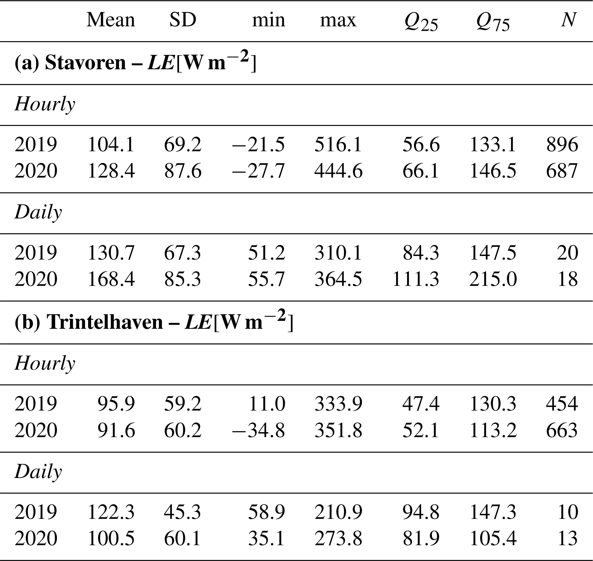

Figure C1An illustration of the decoupling at Trintelhaven in 2019 between the monthly average diurnal cycles of observed latent heat flux (top panels) and global radiation (middle panels), with the latter forming the basis of the frequently used evaporation models of Penman (1948) and Makkink (1957). These models are shown together with the model of Dalton (1802) in the bottom panels. Note that some variables included in the evaporation models are measured at heights above the 2 m that is prescribed (see Eqs. 6–12). Additionally, all three models are generally used on a daily basis, but they are presented here to show the underlying daily cycle. The shaded area represents the uncertainty, which is defined as the standard deviation divided by the square root of the number of observations. Average daily means of the respective variables are indicated by the number in the top left of each panel and display the average course over the summer period.
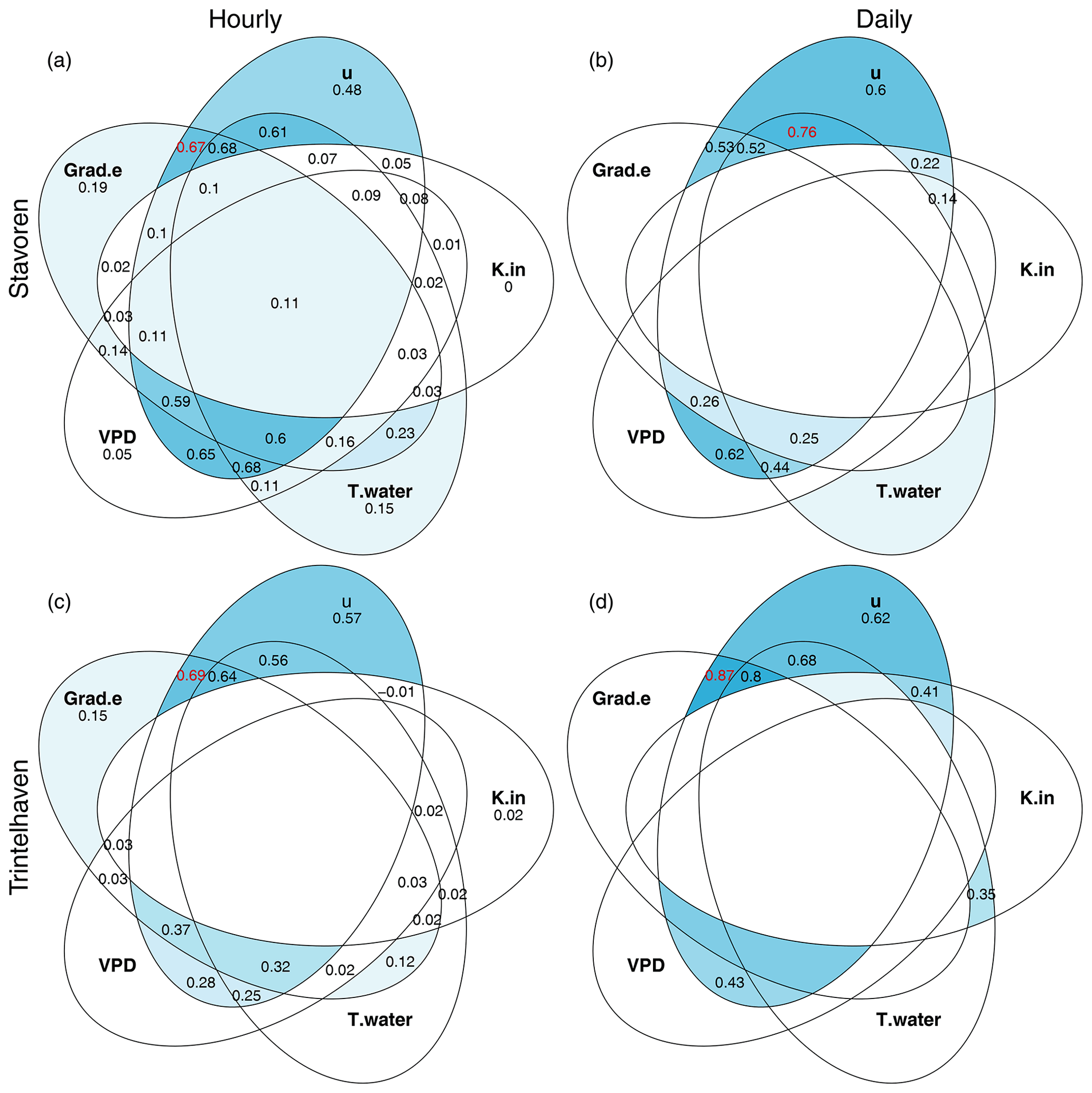
Figure D1A systematic exploration of which variable or combination of variables (product) can best explain the dynamics of open water evaporation. The outer “leaves” of the Venn diagram represent the single variables, whereas the combinations of products of variables are represented towards the centre of the diagram. Within each leaf, the adjusted R2 value is depicted. The higher this value, the bluer the colour of the leaf. The red number indicates the highest R2 value, indicating the best combination found for a maximum of two variables, i.e. the best “simple” model. The R2 values were removed if the model fit was found to be insignificant (p<0.05). The analysis is based on data from the summer of 2019 and is performed at an hourly timescale – Stavoren (a) and Trintelhaven (c) – and a daily timescale – Stavoren (b) and Trintelhaven (d).
Table E1An Analysis of variance (ANOVA) test indicating the significant difference (p<0.05) of the hourly model coefficients found between the two measurement sites during the summer of 2019.
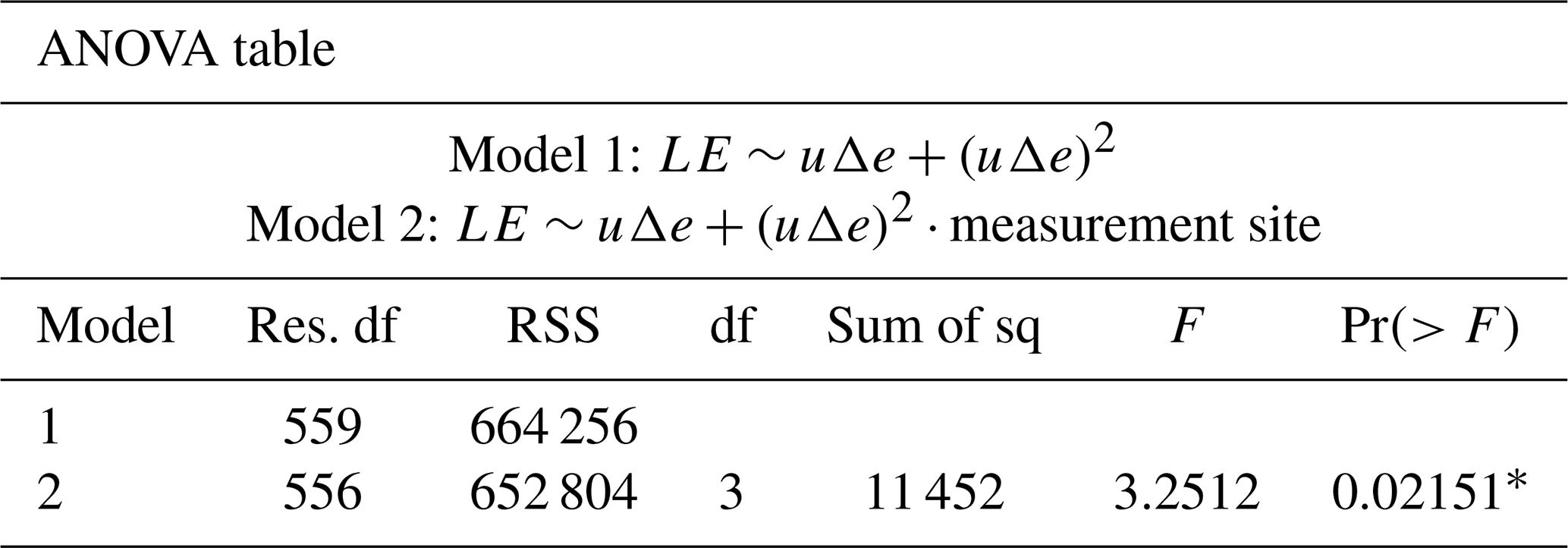
The abbreviations used in the table are as follows: Res. df – residual degrees of freedom, RSS – residual sum of squares, df – degrees of freedom, Sum of sq – sum of squares, F – value of F statistics, and Pr – p value for F statistics. Significance is represented as follows: [0, 0.001] “”; [0.001, 0.01] “”; [0.01, 0.05] “*”; and >0.05 “ ” (no symbol).
The evaporation datasets for Stavoren and Trintelhaven are available on the 4TU.ResearchData repository (https://doi.org/10.4121/16601675; Jansen et al., 2021). The code and accompanying data for the regression analysis are also available on the 4TU.ResearchData repository (https://doi.org/10.4121/16913308; Jansen et al., 2021). The KNMI datasets are available at https://www.knmi.nl/nederland-nu/klimatologie/uurgegevens (KNMI, 2021b). The water temperature datasets of Rijkswaterstaat are available at https://waterinfo.rws.nl/#!/kaart/watertemperatuur/ (Rijkswaterstaat, 2021). The sub-skin Sea Surface Temperature product of the Meteosat-11 satellite is available at https://osi-saf.eumetsat.int/products/sea-surface-temperature-products (EUMETSAT, 2021).
FAJ designed and carried out the study and field work under the supervision of AJT, RU, and CMJJ. All authors contributed to the interpretation of the results. FAJ wrote the manuscript, and AJT, RU, and CMJJ provided feedback on the manuscript.
At least one of the (co-)authors is a member of the editorial board of Hydrology and Earth System Sciences. The peer-review process was guided by an independent editor, and the authors also have no other competing interests to declare.
Publisher's note: Copernicus Publications remains neutral with regard to jurisdictional claims in published maps and institutional affiliations.
The authors would like to thank Pieter Hazenberg for his technical expertise and help in setting up the measurement equipment in Stavoren and Trintelhaven as well as Jelte de Bruin for assistance in the field. Furthermore, the authors are grateful to the three anonymous referees and the handling editor, Stan Schymanski, for valuable feedback during the interactive discussion that helped to improve the manuscript.
This research has been supported by the Dutch Research Council (Nederlandse Organisatie voor Wetenschappelijk Onderzoek; grant no. ALWTW.2016.049).
This paper was edited by Stan Schymanski and reviewed by three anonymous referees.
Abdelrady, A. R., Timmermans, J., Vekerdy, Z., and Salama, M. S.: Surface Energy Balance of Fresh and Saline Waters: AquaSEBS, Remote Sens., 8, 583, https://doi.org/10.3390/rs8070583, 2016. a
Abtew, W. and Melesse, A. M.: Evaporation and Evapotranspiration: Measurements and Estimations, Springer Netherlands, ISBN 978-94-007-4736-4, 2013. a
Adrian, R., O'Reilly, C. M., Zagarese, H., Baines, S. B., Hessen, D. O., Keller, W., Livingstone, D. M., Sommaruga, R., Straile, D., Van Donk, E., Weyhenmeyer, G. A., and Winder, M.: Lakes as Sentinels of Climate Change, Limnol. Oceanogr., 54, 2283–2297, 2009. a
Allen, R. G., Pereira, L. S., Raes, D., and Smith, M.: Crop Evapotranspiration – Guidelines for Computing Crop Water Requirements, FAO Irrigation and Drainage Paper 56, United Nations – Food and Agricultural Organization, https://www.fao.org/3/x0490e/x0490e00.htm (last access: 3 June 2022), 1998. a, b
Bentamy, A., Piollé, J. F., Grouazel, A., Danielson, R., Gulev, S., Paul, F., Azelmat, H., Mathieu, P. P., von Schuckmann, K., Sathyendranath, S., Evers-King, H., Esau, I., Johannessen, J. A., Clayson, C. A., Pinker, R. T., Grodsky, S. A., Bourassa, M., Smith, S. R., Haines, K., Valdivieso, M., Merchant, C. J., Chapron, B., Anderson, A., Hollmann, R., and Josey, S. A.: Review and Assessment of Latent and Sensible Heat Flux Accuracy over the Global Oceans, Remote Sens. Environ., 201, 196–218, https://doi.org/10.1016/j.rse.2017.08.016, 2017. a
Beyrich, F., Bange, J., Hartogensis, O. K., Raasch, S., Braam, M., van Dinther, D., Gräf, D., van Kesteren, B., van den Kroonenberg, A. C., Maronga, B., Martin, S., and Moene, A. F.: Towards a Validation of Scintillometer Measurements: The LITFASS-2009 Experiment, Bound.-Lay. Meteorol., 144, 83–112, https://doi.org/10.1007/s10546-012-9715-8, 2012. a
Blanken, P. D., Rouse, W. R., Culf, A. D., Spence, C., Boudreau, L. D., Jasper, J. N., Kochtubajda, B., Schertzer, W. M., Marsh, P., and Verseghy, D.: Eddy Covariance Measurements of Evaporation from Great Slave Lake, Northwest Territories, Canada, Water Resour. Res., 36, 1069–1077, https://doi.org/10.1029/1999WR900338, 2000. a
Blanken, P. D., Spence, C., Hedstrom, N., and Lenters, J. D.: Evaporation from Lake Superior: 1. Physical Controls and Processes, J. Great Lakes Res., 37, 707–716, https://doi.org/10.1016/j.jglr.2011.08.009, 2011. a, b
Bouin, M.-N., Caniaux, G., Traullé, O., Legain, D., and Moigne, P. L.: Long-Term Heat Exchanges over a Mediterranean Lagoon, J. Geophys. Res.-Atmos., 117, D23104, https://doi.org/10.1029/2012JD017857, 2012. a
Brutsaert, W.: Evaporation into the Atmosphere: Theory, History and Applications, Springer Netherlands, https://doi.org/10.1007/978-94-017-1497-6, 1982. a, b, c, d, e, f, g
Buitelaar, R., Kollen, J., and Leerlooijer, C.: Rapport Operationeel Waterbeheer IJsselmeergebied – Inventarisatie Huidige Waterbeheer IJsselmeergebied Door Rijkswaterstaat En Waterschappen, Tech. rep., Grontmij, Alkmaar, https://www.slimwatermanagement.nl/publish/pages/185213/ijg_20170321_rapport_operationeel_waterbeheer_ijsselmeergebied-n.pdf (last access: 3 June 2022), 2015. a
Christidis, N. and Stott, P. A.: The Influence of Anthropogenic Climate Change on Wet and Dry Summers in Europe, Sci. Bull., 66, 813–823, https://doi.org/10.1016/j.scib.2021.01.020, 2021. a
Cogley, J. G.: The Albedo of Water as a Function of Latitude, Mon. Weather Rev., 107, 775–781, https://doi.org/10.1175/1520-0493(1979)107<0775:TAOWAA>2.0.CO;2, 1979. a
Cronin, M. F., Gentemann, C. L., Edson, J., Ueki, I., Bourassa, M., Brown, S., Clayson, C. A., Fairall, C. W., Farrar, J. T., Gille, S. T., Gulev, S., Josey, S. A., Kato, S., Katsumata, M., Kent, E., Krug, M., Minnett, P. J., Parfitt, R., Pinker, R. T., Stackhouse, P. W. J., Swart, S., Tomita, H., Vandemark, D., Weller, A. R., Yoneyama, K., Yu, L., and Zhang, D.: Air-Sea Fluxes with a Focus on Heat and Momentum, Front. Mar. Sci., 6, 430, https://doi.org/10.3389/fmars.2019.00430, 2019. a
Dalton, J.: Experimental Essays on the Constitution of Mixed Gases: On the Force of Steam or Vapour from Water or Other Liquids in Different Temperatures, Both in a Torricelli Vacuum and in Air; on Evaporation; and on Expansion of Gases by Heat, Memoirs of the Literary and Philosophical Society of Manchester, 5, 536–602, 1802. a, b, c, d, e, f
De Bruin, H. A. R.: Neerslag, Openwaterverdamping En Potentieel Neerslagoverschot in Nederland, Frequentieverdelingen in Het Groeiseizoen, KNMI Report WR 79-04, Tech. rep., KNMI, http://resolver.tudelft.nl/uuid:83a4d23d-a59c-4fcf-8855-0d495b109d96 (last access: 3 June 2022), 1979. a, b
de Bruin, H. A. R.: Temperature and Energy Balance of a Water Reservoir Determined from Standard Weather Data of a Land Station, J. Hydrol., 59, 261–274, https://doi.org/10.1016/0022-1694(82)90091-9, 1982. a
De Bruin, H. A. R. and Keijman, J. Q.: The Priestley-Taylor Evaporation Model Applied to a Large Shallow Lake in The Netherlands, J. Appl. Meteorol., 18, 898–903, 1979. a, b
Desai, A. R., Austin, J. A., Bennington, V., and McKinley, G. A.: Stronger Winds over a Large Lake in Response to Weakening Air-to-Lake Temperature Gradient, Nat. Geosci., 2, 855–858, https://doi.org/10.1038/ngeo693, 2009. a
EasyFlux: EasyFlux DL CR6OP for CR6 and Open-Path Eddy-Covariance System – Product Manual, Campbell Scientific, Inc., https://s.campbellsci.com/documents/us/manuals/easyflux-dl-cr6op.pdf (last access: 3 June 2022), 2017. a
EddyPro: EddyPro® Software (Version 7.0) [Computer Software], LI-COR, Inc, Infrastructure for Measurements of the European Carbon Cycle Consortium, https://www.licor.com/env/support/EddyPro/topics/introduction.html (last access: 3 June 2022), 2021. a
EUMETSAT: Sea Surface Temperature Products|OSI SAF, https://osi-saf.eumetsat.int/products/sea-surface-temperature-products, last access: 20 August 2021. a
Finch, J. and Calver, A.: Methods for the Quantification of Evaporation from Lakes, World Meteorological Organisation's Commission for Hydrology, https://nora.nerc.ac.uk/id/eprint/14359/1/wmoevap_271008.pdf (last access: 3 June 2022), 2008. a
Foken, T.: The Energy Balance Closure Problem: An Overview, Ecol. Appl., 18, 1351–1367, https://doi.org/10.1890/06-0922.1, 2008. a
Foken, T., Gockede, M., Mauder, M., Mahrt, L., Amiro, B., and Munger, W.: Chapter 9 – Post-field Data Quality Control, in: Handbook of Micrometeorology, Springer Science + Business Media, Inc, 181–208, https://doi.org/10.1007/1-4020-2265-4, 2004. a
Foken, T., Leuning, R., Oncley, S. R., Mauder, M., and Aubinet, M.: Corrections and Data Quality Control, in: Eddy Covariance. A Practical Guide to Measurements and Data Analysis, Springer Netherlands, Dordrecht, 85–131, https://doi.org/10.1007/978-94-007-2351-1, 2012. a
Granger, R. J. and Hedstrom, N.: Modelling Hourly Rates of Evaporation from Small Lakes, Hydrol. Earth Syst. Sci., 15, 267–277, https://doi.org/10.5194/hess-15-267-2011, 2011. a, b, c, d
Hargreaves, G. H.: Moisture Availability and Crop Production, T. ASAE, 18, 0980–0984, https://doi.org/10.13031/2013.36722, 1975. a
Huisman, P.: Water in the Netherlands, no. 3 in NHV-Special, Netherlands Institute of Applied Geoscience, Delft, ISBN 90-803565-2-2, https://www.nhv.nu/wp-content/uploads/2021/06/NHVspecial_3_water_in_the_netherlands_1998.pdf (last access: 3 June 2022), 1998. a
Jansen, F. A. and Teuling, A. J.: Evaporation from a Large Lowland Reservoir – (Dis)Agreement between Evaporation Models from Hourly to Decadal Timescales, Hydrol. Earth Syst. Sci., 24, 1055–1072, https://doi.org/10.5194/hess-24-1055-2020, 2020. a, b, c, d
Jansen, F. A., Uijlenhoet, R., Jacobs, C. M. J., and Teuling, A. J.: Open water evaporation of Lake IJssel, data used in the study `Evaporation from a large lowland reservoir – observed dynamics during a warm summer', 4TU.ResearchData [data set], https://doi.org/10.4121/16601675, 2021. a
Jansen, F. A., Uijlenhoet, R., Jacobs, C. M. J., and Teuling, A. J.: Open water evaporation of Lake IJssel, scripts and data used for regression analyses in the study `Evaporation from a large lowland reservoir – observed dynamics during a warm summer', 4TU.ResearchData [data set and code], https://doi.org/10.4121/16913308, 2022. a
Jenny, J.-P., Anneville, O., Arnaud, F., Baulaz, Y., Bouffard, D., Domaizon, I., Bocaniov, S. A., Chèvre, N., Dittrich, M., Dorioz, J.-M., Dunlop, E. S., Dur, G., Guillard, J., Guinaldo, T., Jacquet, S., Jamoneau, A., Jawed, Z., Jeppesen, E., Krantzberg, G., Lenters, J., Leoni, B., Meybeck, M., Nava, V., Nõges, T., Nõges, P., Patelli, M., Pebbles, V., Perga, M.-E., Rasconi, S., Ruetz, C. R., Rudstam, L., Salmaso, N., Sapna, S., Straile, D., Tammeorg, O., Twiss, M. R., Uzarski, D. G., Ventelä, A.-M., Vincent, W. F., Wilhelm, S. W., Wängberg, S.-Å., and Weyhenmeyer, G. A.: Scientists' Warning to Humanity: Rapid Degradation of the World's Large Lakes, J. Great Lakes Res., 46, 686–702, https://doi.org/10.1016/j.jglr.2020.05.006, 2020. a
Josey, S. A., Gulev, S., and Yu, L.: Chapter 5. Exchanges Through the Ocean Surface, in: Ocean Circulation and Climate: A 21st Century Perspective, Elsevier Inc. Chapters, 115–140, ISBN 978-0-12-391851-2, 2013. a
Keijman, J. Q.: The Estimation of the Energy Balance of a Lake from Simple Weather Data, Bound.-Lay. Meteorol., 7, 399–407, https://doi.org/10.1007/BF00240841, 1974. a
Keijman, J. Q. and Koopmans, R. W. R.: A Comparison of Several Methods of Estimating the Evaporation of Lake Flevo, International Association of Hydrological Sciences Publ., 109, 225–232, 1973. a
Kleidon, A. and Renner, M.: An Explanation for the Different Climate Sensitivities of Land and Ocean Surfaces Based on the Diurnal Cycle, Earth Syst. Dynam., 8, 849–864, https://doi.org/10.5194/esd-8-849-2017, 2017. a, b
Kljun, N., Calanca, P., Rotach, M. W., and Schmid, H. P.: A Simple Parameterisation for Flux Footprint Predictions, Bound.-Lay. Meteorol., 112, 503–523, https://doi.org/10.1023/B:BOUN.0000030653.71031.96, 2004. a
Kljun, N., Calanca, P., Rotach, M. W., and Schmid, H. P.: A Simple Two-Dimensional Parameterisation for Flux Footprint Prediction (FFP), Geosci. Model Dev., 8, 3695–3713, https://doi.org/10.5194/gmd-8-3695-2015, 2015. a, b
KNMI: KNMI'14 Klimaatscenario's Voor Nederland; Leidraad Voor Professionals in Klimaatadaptatie, Tech. rep., KNMI, De Bilt, https://cdn.knmi.nl/system/data_center_publications/files/000/070/616/original/Brochure_KNMI14_NL.pdf?1640271317 (last access: 3 June 2022), 2015. a
KNMI: KNMI – Klimaatviewer, https://www.knmi.nl/klimaat-viewer/grafieken-tabellen/klimaattabellen-per-station (last access: 1 June 2021), 2021a. a
KNMI: KNMI – Uurgegevens van Het Weer in Nederland, https://www.knmi.nl/nederland-nu/klimatologie/uurgegevens (last access: 20 August 2021), 2021b. a
Le Moigne, P., Colin, J., and Decharme, B.: Impact of Lake Surface Temperatures Simulated by the FLake Scheme in the CNRM-CM5 Climate Model, Tellus A, 68, 31274, https://doi.org/10.3402/tellusa.v68.31274, 2016. a
Lenters, J. D., Kratz, T. K., and Bowser, C. J.: Effects of Climate Variability on Lake Evaporation: Results from a Long-Term Energy Budget Study of Sparkling Lake, Northern Wisconsin (USA), J. Hydrol., 308, 168–195, https://doi.org/10.1016/j.jhydrol.2004.10.028, 2005. a, b
Liu, H., Zhang, Y., Liu, S., Jiang, H., Sheng, L., and Williams, Q. L.: Eddy Covariance Measurements of Surface Energy Budget and Evaporation in a Cool Season over Southern Open Water in Mississippi, J. Geophys. Res.-Atmos., 114, D04110, https://doi.org/10.1029/2008JD010891, 2009. a
Liu, H., Blanken, P. D., Weidinger, T., Nordbo, A., and Vesala, T.: Variability in Cold Front Activities Modulating Cool-Season Evaporation from a Southern Inland Water in the USA, Environ. Res. Lett., 6, 024022, https://doi.org/10.1088/1748-9326/6/2/024022, 2011. a
MacIntyre, S., Fram, J. P., Kushner, P. J., Bettez, N. D., O'Brien, W. J., Hobbie, J. E., and Kling, G. W.: Climate-Related Variations in Mixing Dynamics in an Alaskan Arctic Lake, Limnol. Oceanogr., 54, 2401–2417, https://doi.org/10.4319/lo.2009.54.6_part_2.2401, 2009. a
Makkink, G. F.: Testing the Penman Formula by Means of Lysimeters, J. Inst. Water Eng., 11, 277–288, 1957. a, b, c, d, e, f, g, h
Mammarella, I., Nordbo, A., Rannik, Ü., Haapanala, S., Levula, J., Laakso, H., Ojala, A., Peltola, O., Heiskanen, J., Pumpanen, J., and Vesala, T.: Carbon Dioxide and Energy Fluxes over a Small Boreal Lake in Southern Finland, J. Geophys. Res.-Biogeo., 120, 1296–1314, https://doi.org/10.1002/2014JG002873, 2015. a
Masoner, J. R. and Stannard, D. I.: A Comparison of Methods for Estimating Open-Water Evaporation in Small Wetlands, Wetlands, 30, 513–524, https://doi.org/10.1007/s13157-010-0041-y, 2010. a
Massman, W. J.: A Simple Method for Estimating Frequency Response Corrections for Eddy Covariance Systems, Agr. Forest Meteorol., 104, 185–198, https://doi.org/10.1016/S0168-1923(00)00164-7, 2000. a
Mauder, M., Cuntz, M., Drüe, C., Graf, A., Rebmann, C., Schmid, H. P., Schmidt, M., and Steinbrecher, R.: A Strategy for Quality and Uncertainty Assessment of Long-Term Eddy-Covariance Measurements, Agr. Forest Meteorol., 169, 122–135, https://doi.org/10.1016/j.agrformet.2012.09.006, 2013. a, b
Mauder, M., Foken, T., and Cuxart, J.: Surface-Energy-Balance Closure over Land: A Review, Bound.-Lay. Meteorol., 177, 395–426, https://doi.org/10.1007/s10546-020-00529-6, 2020. a
McGloin, R., McGowan, H., McJannet, D., Cook, F., Sogachev, A., and Burn, S.: Quantification of Surface Energy Fluxes from a Small Water Body Using Scintillometry and Eddy Covariance, Water Resour. Res., 50, 494–513, https://doi.org/10.1002/2013WR013899, 2014. a, b, c
McJannet, D. L., Cook, F. J., McGloin, R. P., McGowan, H. A., and Burn, S.: Estimation of Evaporation and Sensible Heat Flux from Open Water Using a Large-Aperture Scintillometer, Water Resour. Res., 47, W05545, https://doi.org/10.1029/2010WR010155, 2011. a
McMahon, T. A., Peel, M. C., Lowe, L., Srikanthan, R., and McVicar, T. R.: Estimating actual, potential, reference crop and pan evaporation using standard meteorological data: a pragmatic synthesis, Hydrol. Earth Syst. Sci., 17, 1331–1363, https://doi.org/10.5194/hess-17-1331-2013, 2013. a
McVicar, T. R., Roderick, M. L., Donohue, R. J., Li, L. T., Van Niel, T. G., Thomas, A., Grieser, J., Jhajharia, D., Himri, Y., Mahowald, N. M., Mescherskaya, A. V., Kruger, A. C., Rehman, S., and Dinpashoh, Y.: Global Review and Synthesis of Trends in Observed Terrestrial Near-Surface Wind Speeds: Implications for Evaporation, J. Hydrol., 416, 182–205, https://doi.org/10.1016/j.jhydrol.2011.10.024, 2012. a
Metzger, J., Nied, M., Corsmeier, U., Kleffmann, J., and Kottmeier, C.: Dead Sea Evaporation by Eddy Covariance Measurements vs. Aerodynamic, Energy Budget, Priestley–Taylor, and Penman Estimates, Hydrol. Earth Syst. Sci., 22, 1135–1155, https://doi.org/10.5194/hess-22-1135-2018, 2018. a
Mironov, D. V.: Parameterization of Lakes in Numerical Weather Prediction – Description of a Lake Model, COSMO Technical Report No. 11, Deutscher Wetterdienst, Offenback am Main, Germany, https://www.dwd.de/EN/ourservices/cosmo_technical_reports/pdf_einzelbaende/2019_11.pdf;jsessionid=E6ABACC01B5C307215EF0109AF5F4E0A.live21072?__blob=publicationFile&v=2 (last access: 3 June 2022), 2008. a, b, c
Moene, A. F. and van Dam, J. C.: Transport in the Atmosphere-Vegetation-Soil Continuum, Cambridge University Press, https://doi.org/10.1017/CBO9781139043137, 2014. a
Moncrieff, J., Clement, R., Finnigan, J., and Meyers, T.: Averaging, Detrending, and Filtering of Eddy Covariance Time Series, in: Handbook of Micrometeorology: A Guide for Surface Flux Measurement and Analysis, Atmospheric and Oceanographic Sciences Library,edited by: Lee, X., Massman, W., and Law, B., Springer Netherlands, Dordrecht, 7–31, https://doi.org/10.1007/1-4020-2265-4_2, 2004. a
Nordbo, A., Launiainen, S., Mammarella, I., Leppäranta, M., Huotari, J., Ojala, A., and Vesala, T.: Long-Term Energy Flux Measurements and Energy Balance over a Small Boreal Lake Using Eddy Covariance Technique, J. Geophys. Res.-Atmos., 116, D02119, https://doi.org/10.1029/2010JD014542, 2011. a, b, c
Penman, H. L.: Natural Evaporation from Open Water, Bare Soil and Grass, P. Roy. Soc. Lond. A, 193, 120–145, https://doi.org/10.1098/rspa.1948.0037, 1948. a, b, c, d, e, f, g, h, i
Penman, H. L.: Evaporation: An Introductory Survey, Neth. J. Agricult. Sci., 4, 9–29, https://doi.org/10.18174/njas.v4i1.17768, 1956. a
Pinker, R. T., Bentamy, A., Katsaros, K. B., Ma, Y., and Li, C.: Estimates of Net Heat Fluxes over the Atlantic Ocean, J. Geophys. Res.-Oceans, 119, 410–427, https://doi.org/10.1002/2013JC009386, 2014. a
Potes, M., Salgado, R., Costa, M. J., Morais, M., Bortoli, D., Kostadinov, I., and Mammarella, I.: Lake–Atmosphere Interactions at Alqueva Reservoir: A Case Study in the Summer of 2014, Tellus A, 69, 1272787, https://doi.org/10.1080/16000870.2016.1272787, 2017. a
Priestley, C. H. B. and Taylor, R. J.: On the Assessment of Surface Heat Flux and Evaporation Using Large-Scale Parameters, Mon. Weather Rev., 100, 81–92, https://doi.org/10.1175/1520-0493(1972)100<0081:OTAOSH>2.3.CO;2, 1972. a
Rijkswaterstaat: Watertemperatuur – Rijkswaterstaat, https://waterinfo.rws.nl/#!/kaart/watertemperatuur/, last access: 20 August 2021. a
Schmid, M. and Köster, O.: Excess Warming of a Central European Lake Driven by Solar Brightening, Water Resour. Res., 52, 8103–8116, https://doi.org/10.1002/2016WR018651, 2016. a
Schotanus, P., Nieuwstadt, F., and De Bruin, H.: Temperature Measurement with a Sonic Anemometer and Its Application to Heat and Moisture Fluxes, Bound.-Lay. Meteorol., 26, 81–93, https://doi.org/10.1007/BF00164332, 1983. a
Seneviratne, S. I., Lüthi, D., Litschi, M., and Schär, C.: Land–Atmosphere Coupling and Climate Change in Europe, Nature, 443, 205–209, https://doi.org/10.1038/nature05095, 2006. a
Seneviratne, S. I., Nicholls, N., Easterling, D., Goodess, C. M., Kanae, S., Kossin, J., Luo, Y., Marengo, J., McInnes, K., Rahimi, M., Reichstein, M., Sorteberg, A., Vera, C., Zhang, X., Rusticucci, M., Semenov, V., Alexander, L. V., Allen, S., Benito, G., Cavazos, T., Clague, J., Conway, D., Della-Marta, P. M., Gerber, M., Gong, S., Goswami, B. N., Hemer, M., Huggel, C., van den Hurk, B., Kharin, V. V., Kitoh, A., Tank, A. M. K., Li, G., Mason, S., McGuire, W., van Oldenborgh, G. J., Orlowsky, B., Smith, S., Thiaw, W., Velegrakis, A., Yiou, P., Zhang, T., Zhou, T., and Zwiers, F. W.: Changes in Climate Extremes and Their Impacts on the Natural Physical Environment, in: Managing the Risks of Extreme Events and Disasters to Advance Climate Change Adaptation, edited by: Field, C. B., Barros, V., Stocker, T. F., and Dahe, Q., Cambridge University Press, Cambridge, 109–230, https://doi.org/10.1017/CBO9781139177245.006, 2012. a
Sumner, D. M. and Jacobs, J. M.: Utility of Penman–Monteith, Priestley–Taylor, Reference Evapotranspiration, and Pan Evaporation Methods to Estimate Pasture Evapotranspiration, J. Hydrol., 308, 81–104, https://doi.org/10.1016/j.jhydrol.2004.10.023, 2005. a
Tanny, J., Cohen, S., Assouline, S., Lange, F., Grava, A., Berger, D., Teltch, B., and Parlange, M. B.: Evaporation from a Small Water Reservoir: Direct Measurements and Estimates, J. Hydrol., 351, 218–229, https://doi.org/10.1016/j.jhydrol.2007.12.012, 2008. a, b, c
Teuling, A. J.: A Hot Future for European Droughts, Nat. Clim. Change, 8, 364–365, https://doi.org/10.1038/s41558-018-0154-5, 2018. a
van Emmerik, T., Rimmer, A., Lechinsky, Y., Wenker, K., Nussboim, S., and van de Giesen, N.: Measuring Heat Balance Residual at Lake Surface Using Distributed Temperature Sensing: Measuring Lake Heat Balance Residual Using DTS, Limnol. Oceanogr.: Meth., 11, 79–90, https://doi.org/10.4319/lom.2013.11.79, 2013. a
Venäläinen, A., Frech, M., Heikinheimo, M., and Grelle, A.: Comparison of Latent and Sensible Heat Fluxes over Boreal Lakes with Concurrent Fluxes over a Forest: Implications for Regional Averaging, Agr. Forest Meteorol., 98–99, 535–546, https://doi.org/10.1016/S0168-1923(99)00100-8, 1999. a, b
Vesala, T., Huotari, J., Rannik, Ü., Suni, T., Smolander, S., Sogachev, A., Launiainen, S., and Ojala, A.: Eddy Covariance Measurements of Carbon Exchange and Latent and Sensible Heat Fluxes over a Boreal Lake for a Full Open-Water Period, J. Geophys. Res.-Atmos., 111, D11101, https://doi.org/10.1029/2005JD006365, 2006. a
Vickers, D. and Mahrt, L.: Quality Control and Flux Sampling Problems for Tower and Aircraft Data, J. Atmos. Ocean. Tech., 14, 512–526, https://doi.org/10.1175/1520-0426(1997)014<0512:QCAFSP>2.0.CO;2, 1997. a
Voskamp, T.: The Evaporation of Lake IJssel – Comparison of the FLake Model with Standard Methods at Multiple Timescales for Estimating Evaporation Rates, MSc thesis report, Wageningen University, Wageningen, 2018. a
Wang, W., Xiao, W., Cao, C., Gao, Z., Hu, Z., Liu, S., Shen, S., Wang, L., Xiao, Q., Xu, J., Yang, D., and Lee, X.: Temporal and Spatial Variations in Radiation and Energy Balance across a Large Freshwater Lake in China, J. Hydrol., 511, 811–824, https://doi.org/10.1016/j.jhydrol.2014.02.012, 2014. a
Wang, W., Lee, X., Xiao, W., Liu, S., Schultz, N., Wang, Y., Zhang, M., and Zhao, L.: Global Lake Evaporation Accelerated by Changes in Surface Energy Allocation in a Warmer Climate, Nat. Geosci., 11, 410–414, https://doi.org/10.1038/s41561-018-0114-8, 2018. a, b, c, d
Webb, E. K., Pearman, G. I., and Leuning, R.: Correction of Flux Measurements for Density Effects Due to Heat and Water Vapour Transfer, Q. J. Roy. Meteorol. Soc., 106, 85–100, https://doi.org/10.1002/qj.49710644707, 1980. a
Weisman, R. N. and Brutsaert, W.: Evaporation and Cooling of a Lake under Unstable Atmospheric Conditions, Water Resources Research, 9, 1242–1257, https://doi.org/10.1029/WR009i005p01242, 1973. a
Wilczak, J. M., Oncley, S. P., and Stage, S. A.: Sonic Anemometer Tilt Correction Algorithms, Bound.-Lay. Meteorol., 99, 127–150, https://doi.org/10.1023/A:1018966204465, 2001. a
Wilson, K., Goldstein, A., Falge, E., Aubinet, M., Baldocchi, D., Berbigier, P., Bernhofer, C., Ceulemans, R., Dolman, H., Field, C., Grelle, A., Ibrom, A., Law, B. E., Kowalski, A., Meyers, T., Moncrieff, J., Monson, R., Oechel, W., Tenhunen, J., Valentini, R., and Verma, S.: Energy Balance Closure at FLUXNET Sites, Agr. Forest Meteorol., 113, 223–243, https://doi.org/10.1016/S0168-1923(02)00109-0, 2002. a, b
Woolway, R. I., Verburg, P., Lenters, J. D., Merchant, C. J., Hamilton, D. P., Brookes, J., de Eyto, E., Kelly, S., Healey, N. C., Hook, S., Laas, A., Pierson, D., Rusak, J. A., Kuha, J., Karjalainen, J., Kallio, K., Lepistö, A., and Jones, I. D.: Geographic and Temporal Variations in Turbulent Heat Loss from Lakes: A Global Analysis across 45 Lakes, Limnol. Oceanogr., 63, 2436–2449, https://doi.org/10.1002/lno.10950, 2018. a
Woolway, R. I., Kraemer, B. M., Lenters, J. D., Merchant, C. J., O'Reilly, C. M., and Sharma, S.: Global Lake Responses to Climate Change, Nat. Rev. Earth Environ., 1, 388–403, https://doi.org/10.1038/s43017-020-0067-5, 2020. a, b, c, d, e
Zhou, W., Wang, L., Li, D., and Leung, L. R.: Spatial Pattern of Lake Evaporation Increases under Global Warming Linked to Regional Hydroclimate Change, Commun. Earth Environ., 2, 1–10, https://doi.org/10.1038/s43247-021-00327-z, 2021. a