Performance-based comparison of regionalization methods to improve the at-site estimates of daily precipitation

In this article, we compare the performance of three regionalization approaches in improving the at-site estimates of daily precipitation. The first method is built on the idea of conventional RFA (regional frequency analysis) but is based on a fast algorithm that defines distinct homogeneous regions relying on their upper-tail similarity. It uses only the precipitation data at hand without the need for any additional covariate. The second is based on the region-of-influence (ROI) approach in which neighborhoods, containing similar sites, are defined for each station. The third is a spatial method that adopts generalized additive model (GAM) forms for the model parameters. In line with our goal of modeling the whole range of positive precipitation, the chosen marginal distribution model is the extended generalized Pareto distribution (EGPD) to which we apply the three methods. We consider a dense network composed of 1176 daily stations located within Switzerland and in neighboring countries. We compute different criteria to assess the models' performance in the bulk of the distribution and the upper tail. The results show that all the regional methods offered improved robustness over the local EGPD model. While the GAM method is more robust and reliable in the upper tail, the ROI method is better in the bulk of the distribution.

1 Introduction

Flood events occurring at different timescales pose hazards that are of enormous consequences for life and property. Even though necessary for risk assessments and safe design, reliable prediction remains a challenge and a difficult task. Usually, in the context of risk assessment, river flows are simulated via hydrological models. These models take as inputs, among others, meteorological data such as temperature and precipitation. However, whatever the complexity of the model and how it represents the underlying hydrological behavior of the catchment, the accuracy, robustness, and reliability of the flood predictions rely on the quality of the input data.

Precipitation intensities, the key input signal, are modeled using probabilistic methods. Within this framework, a good probabilistic model should predict rainfall intensities of any return level, whether low, medium, or extreme, with reliable accuracy. Gamma distribution, a common choice over models such as log-normal, Weibull, and exponential, fails in this respect, as the tail is too light to model heavy intensities (Katz et al., 2002). Models based on the classical extreme value theory (EVT), such as generalized Pareto (GP), can model the upper tail, but one has to choose another model for the other intensities below the chosen threshold.

Since generalized Pareto distribution (GPD) has been favored in hydrological applications (see, e.g., Langousis et al., 2016), many authors in the framework of modeling the full range of observations have considered different approaches to adding flexibility to this model. A common approach is the use of mixture models where GPD is combined with another appropriate model for the bulk of the distribution (see the review in Scarrot and MacDonald, 2012). Mixture models, however, have the drawback of inflating the number of parameters to estimate (Naveau et al., 2016) and thus complexify statistical inference.

As an alternative, Naveau et al. (2016) proposed a model which is an extension of the GP (afterward called extended generalized Pareto distribution – EGPD). It has the advantage of avoiding the need for threshold selection (a drawback of GP) while being parsimonious by avoiding the use of mixtures. The model is Gamma-like in the lower tail and heavy-tailed (GP) in the upper tail, with a smooth transition in between. It is able to model adequately the entire range of positive precipitation, and many authors within the framework of rainfall modeling have used this model (e.g., Blanchet et al., 2015; Evin et al., 2018; Tencaliec et al., 2020; Le Gall et al., 2022).

Modeling the whole range of precipitation has various practical applications. For instance, in flood risk assessments, where stochastic precipitation generators are used to simulate long series of positive precipitation, extremes included (e.g., in Evin et al., 2018). The simulated precipitation is then used as input to conceptual hydrological models for the simulation of long series of river flows. Other practical applications are in the evaluation of numerical weather simulations or investigation of the climatology of rainfall events as outlined by Blanchet et al. (2019).

Although EGPD uses all the data to estimate the parameters, the shape parameter which controls the upper-tail behavior remains difficult to estimate based on a few decades of data, the usual length of precipitation data. This is because there are usually few extremes exhibiting much variability. As precipitation is spatial by nature, several studies (Cunnane, 1988; Burn, 1990; Hosking and Wallis, 2005) proposed the use of observations surrounding the local station to increase the number of data available for estimation, thereby reducing the uncertainty involved in the estimation.

Different methods exist in the literature to use information surrounding the station at hand (see Cunnane, 1988; Hosking and Wallis, 2005). Methods based on regional homogeneity (e.g., the method of Hosking and Wallis, 2005) pool all observations in hydrologically similar sites to increase the sample size and so yield more accurate estimates of the parameters. Hydrologically similar sites are first defined using cluster analysis and are then subjected to some statistical homogeneity tests on the scaled observations. Thereafter, a chosen distribution is fitted to the scaled observations in the identified region, and all stations within this region would share the same regional parameters. Station-specific parameters and quantiles can then be inferred by appropriate scaling. This method has been applied by various authors (e.g., Gaál and Kyselý, 2009; Malekinezhad and Zare-Garizi, 2014) and to various distributions such as the GEV and GP. Variants of this method exist, such as the region of influence (ROI) proposed by Burn (1990), which avoids defining fixed regions but assigns homogeneous regions (neighborhood of different shapes according to the method) for each site. Scaled observations within the neighborhood of each station are then used to estimate the regional parameters of that station. This method has been applied by various authors (see Gaál et al., 2008; Kyselý et al., 2011; Carreau et al., 2013; Evin et al., 2016; Das, 2017, 2019).

In contrast to the aforementioned methods that generally rely on some covariates such as spatial coordinates to define the homogeneous regions, another variant, recently developed by Le Gall et al. (2022), defines homogeneous regions based on the similarity of their upper-tail behavior. This method avoids the use of any covariate but relies completely on the precipitation data at hand. The upper-tail behavior for each station is summarized based on a ratio of probability-weighted moments (PWMs) (refer to Eq. 4). Subsequently, a clustering algorithm is used to partition these ratios into distinct homogeneous regions, and then regional parameters can be estimated.

Spatial methods exist in which all the observations from all the stations are pooled and then used to estimate the spatial surface for each of the model parameters. The surface for each of the model parameters is defined as a function of some well-chosen covariates such as longitude, latitude, or altitude. Estimating the parameters involves simply the estimation of the coefficients of these relationships. From the fitted surfaces, station-specific model parameters can be inferred as a function of the covariates at that specific location. Surfaces that are smooth and flexible can be obtained by fitting generalized additive models (GAMs) to the relationships (see Chavez-Demoulin and Davison, 2005; Blanchet and Lehning, 2010; Youngman, 2019, 2020). Other alternatives to the classical RFA include the Bayesian spatial modeling (see Madsen et al., 1995; Cooley et al., 2007) and those discussed in Cunnane (1988).

Recent analyses have been done to compare the performance of regional approaches with a particular interest in distributions allowing one to model extremes only. Gaál et al. (2008) compared different versions of the ROI method against the classical RFA method of Hosking and Wallis (2005). The ROI versions were distinguished by the choice of the distance metric and the maximum threshold to delineate neighborhoods. For all the methods, GEV distribution was assumed to be the underlying distribution. The authors, through a Monte Carlo simulation study, concluded that the ROI approach was superior to the classical RFA involving distinct clusters. In an interpolation framework, Carreau et al. (2013) compared three methods: spatial interpolation of locally estimated parameters, the ROI method, and a rainfall generator called SHYPRE. For the first two methods, GEV distribution was assumed. The authors found comparable performance between the ROI and SHYPRE and a lack of robustness in the method based on interpolation of local parameters. Deidda et al. (2021) also used GEV to compare the classical RFA of Hosking and Wallis (2005) and geostatistical interpolation of locally estimated parameters. They highlighted the limitation of the former in yielding distinct regions and being of less accuracy compared to the latter. Other comparisons include those of Gaál and Kyselý (2009), Kyselý et al. (2011), and Das (2019).

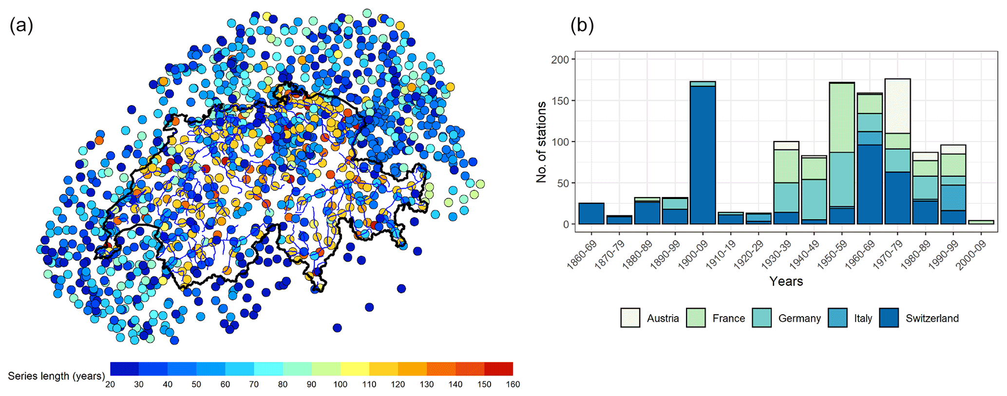
Figure 1 Description of the data used for the study. (a) Map of Switzerland and the neighboring areas showing the locations of the 1176 daily stations. The color indicates the length of the series, a minimum of 20 years and a maximum of 156 years. (b) Bar plot showing the number of stations installed in each country for each decade.

Our approach differs from the aforementioned studies in the following respects. First, in contrast to the case where the underlying distributions are basically for modeling only extremes (e.g., Burn, 1990; Gaál et al., 2008; Gaál and Kyselý, 2009; Kyselý et al., 2011; Carreau et al., 2013; Evin et al., 2016; Das, 2019; Deidda et al., 2021), we consider the EGPD that models low, medium, and extreme precipitations. This is in line with our goal of having a robust and reliable model that can model the whole distribution and not only the extremes. Secondly, our comparison approach is more general and is based on Garavaglia et al. (2011) and Renard et al. (2013), focusing on the predictive ability of the models in a cross-validation framework similar to the case of authors such as Blanchet et al. (2015) and Evin et al. (2016) rather than simply based on quality of fit (e.g., Gaál et al., 2008; Kyselý et al., 2011; Deidda et al., 2021). Finally, in our contribution, we compare new methods not previously compared viz-a-viz. The first method defines distinct homogeneous regions based on their similarity in upper-tail behavior (Le Gall et al., 2022). The second method is based on the ROI approach framework of Evin et al. (2016). The last method is a spatial approach that assumes the GAM forms for the model parameters. For all the methods, we assume the EGPD to be the underlying marginal distribution. We apply this comparison to a dense network of over 1100 daily stations located within Switzerland and in the neighboring countries.

The paper is organized as follows: Sect. 2 presents the data and the study area. Section 3 introduces the competing models, while Sect. 4 describes the comparison methodology as well as the criteria used. The results are presented in Sect. 5. Finally, we discuss the conclusion and the relevant perspectives in Sect. 6.

2 Data and study area

The comparison is made considering daily precipitation observations from 1176 stations shown in Fig. 1. Of this total, 500 are located within Switzerland and 676 in the neighboring countries. The data have a variable length ranging from a minimum of 20 years to a maximum of 156 years, from 1863 to 2019. The bar plot in Fig. 1 shows the number of stations installed in each country during each decade of the study period. While the main study area is Switzerland, we use the data in the neighboring countries simply to improve the estimates of the stations located around the border of Switzerland. Consequently, although we use all the stations (both within and outside) for regionalization and model fitting, we apply the performance criteria only to the stations located in Switzerland.

Daily precipitation in Switzerland is characterized by seasonality arising from multiple moisture sources brought by prevailing winds (Sodemann and Zubler, 2009; Umbricht et al., 2013; Giannakaki and Martius, 2015). It is also characterized by spatial variability in both intensity and occurrence resulting from the complex topography (Sevruk, 1997; Sevruk et al., 1998; Frei and Scha, 1998; Molnar and Burlando, 2008; Isotta et al., 2014). Winter receives the least precipitation, and summer is the main season of precipitation all over Switzerland. An exception is in the case of Ticino in the south, where fall is the main season. This region is also subject to the heaviest precipitation. In the north of the country, the topography plays an important role: the northern rim and the Jura mountains receive heavier precipitation compared to the plateau.

As a result of the marked seasonality and the importance of taking it into account (Leonard et al., 2008; Garavaglia et al., 2011), we apply a seasonally based analysis approach. We divide the data into the four distinct seasons of 3 months each: winter (December, January, February), spring (March, April, May), summer (June, July, August), and fall (September, October, November).

3 Candidate methods

In this section, we start by presenting the marginal distribution (EGPD). We then give a brief description of three different methods of regionalization that we will use to improve the local estimates of the EGPD. They are (i) regional frequency analysis based on the upper-tail behavior, (ii) the ROI approach, and (iii) the spatial method using GAM forms. Finally, we summarize the regional models that are developed based on the three outlined methods of regionalization as applied to the EGPD.

3.1 Marginal distribution of positive rainfall

We use the marginal distribution of rainfall proposed by Naveau et al. (2016), which is able to model sufficiently the full spectrum of positive (non-zero) rainfall. The model is EVT compliant in the upper and lower tails while providing a smooth transition in between. It provides an alternative to the light-tailed distributions such as Gamma, which can underestimate extremes (Katz et al., 2002). Four parametric families of this model have been proposed by Naveau et al. (2016) and more recently a non-parametric scheme of the transition function by Tencaliec et al. (2020). However, the simplest of the parametric family is parsimonious and can adequately model precipitation intensities without the need for GPD threshold selection (Naveau et al., 2016; Evin et al., 2018; Le Gall et al., 2022). We therefore use this model in our study.

Let X be a random variable representing positive daily precipitation intensity that is distributed according to the EGPD; then, the cumulative distribution function (CDF) is given by

$$\begin{array}{}\text{(1)}& F\left(x\right)=\mathbb{P}(X\le x)=G\left[H_{\mathit{\xi }}\left({\displaystyle \frac{x}{\mathit{\sigma }}}\right)\right],\end{array}$$

where G is any CDF that ensures a smooth transition between the EVT-compliant upper and lower tails, and

$$\begin{array}{}\text{(2)}& H_{\mathit{\xi }}\left({\displaystyle \frac{x}{\mathit{\sigma }}}\right)=\left\{\begin{array}{ll}\mathrm{1}-(\mathrm{1}+\mathit{\xi }\frac{x}{\mathit{\sigma }}{)}_{+}^{-\mathrm{1}/\mathit{\xi }}& \text{ if }\mathit{\xi }\ne \mathrm{0},\\ \mathrm{1}-\exp (-x/\mathit{\sigma })& \text{ if }\mathit{\xi }=\mathrm{0},\end{array}\right.\end{array}$$

with $a_{+}=max(a,\mathrm{0})$.

For the parsimonious model we use, the function G is simply defined as G(v)=v^k. Therefore, the model is given as

$$\begin{array}{}\text{(3)}& F\left(x\right)={\left[H_{\mathit{\xi }}\left({\displaystyle \frac{x}{\mathit{\sigma }}}\right)\right]}^k.\end{array}$$

The model has three parameters. k>0 controls the lower tail, ξ≥0 controls the upper tail, and σ>0 is the scale parameter.

Inference of the model parameters can be done through maximum likelihood estimation (MLE) or through the method of PWMs.

3.2 Methods of regionalization

3.2.1 RFA based on upper-tail behavior

Classical regional frequency analysis (Hosking and Wallis, 2005) defines regions that are homogeneous up to a scaling factor. To identify the regions, covariates have to be carefully chosen, which usually include at-site characteristics such as geographical and atmospheric characteristics. However, this information might not be generally available at each station. Homogeneity tests then have to be applied to confirm that the regions are sufficiently similar.

Le Gall et al. (2022) proposed a fast and efficient method to delineate regions based on the homogeneity of their upper-tail behavior. The method relies on the precipitation data at hand, only without the need for additional covariates. More so, regions identified are inherently homogeneous, thereby avoiding the need for the application of some homogeneity tests. For each station i, a ratio ω given in Eq. (4) that is based on PWMs is obtained.

$$\begin{array}{}\text{(4)}& \widehat{\mathit{\omega }}={\displaystyle \frac{\mathrm{3}{\widehat{\mathit{\alpha }}}_{\mathrm{2}}-{\widehat{\mathit{\alpha }}}_{\mathrm{0}}}{\mathrm{2}\widehat{{\mathit{\alpha }}_{\mathrm{1}}}-{\widehat{\mathit{\alpha }}}_{\mathrm{0}}}}-\mathrm{1},\end{array}$$

where ${\widehat{\mathit{\alpha }}}_j$ denotes the PWM of order j.

The authors showed that ω summarizes the upper-tail behavior of the data at hand, and for the EGPD model, this depends mainly on the ξ parameter (the effect of k is not very significant; see Le Gall et al., 2022). Stations with high values of ω have high intense extremes, and those with low values have less intense extremes. The idea is to classify or form regions with similar values of ω, which is possible using any of the clustering algorithms, such as K-means, hierarchical clustering, or partitioning around medoids (PAM). For details of these clustering methods, see Kaufman and Rousseeuw (2005).

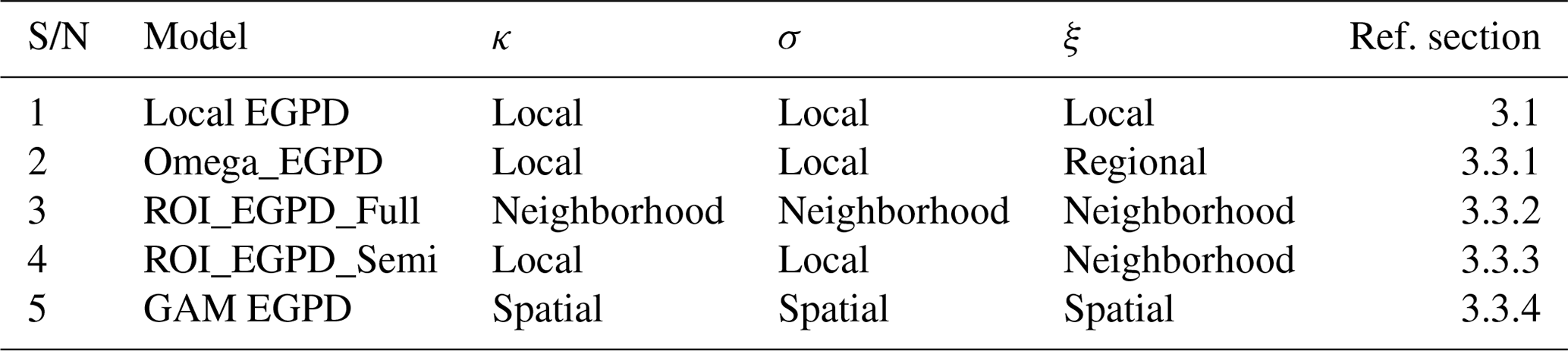
Table 1 Summary of the regional models that are compared in this study. The first model is the local EGPD model, the next three models are based on regional homogeneity, and the last model is a spatial method based on GAM. The second column gives the name of the model. The next three columns are the parameters of the EGPD model and indicate whether the parameter is estimated locally (from the data of the station at hand only) or through regionalization. The last column gives a reference to the section where the method is described.

3.2.2 RFA based on the ROI approach

The ROI method (Burn, 1990) is similar in concept to the classical RFA method. It circumvents the drawback of having contiguous regions separated by distinct boundaries that result in “undesirable step changes of the variables and estimated quantiles” (Gaál et al., 2008). Instead of defining distinct homogeneous regions separated by some boundaries, a region of influence is assigned to each station. All the scaled observations in the identified ROI are used to estimate its regional parameters. To apply this method, several choices have to be made. These involve the choice of the scale factor, distance metric, radius delimitation, and homogeneity test. The choices influence the application of the method and have to be carefully and objectively decided on. Different authors in the application of the methods have explored some or all of these factors, starting from Burn (1990) and in Gaál et al. (2008).

In this work, we follow the objectively selected steps and choices similarly to Evin et al. (2016) in the application of the method in the southeastern part of France. The authors applied the method by considering peaks over threshold (POT) (exceedances of a 70 % quantile) of central rainfalls (largest observations in 3 d rainfall events) and of some distributions (exponential, GPD, and Weibull). We apply the same procedure but to positive rainfall and the EGPD model.

3.2.3 Spatial method based on the GAM

In contrast to the previous methods where regionalization is based on homogeneity of normalized data or upper-tail similarity, this is a regression-based method for fitting the parameters of models by allowing for spatial non-stationarity of the parameters. Accordingly, we pool all the observations from all the stations to estimate flexible and smooth spatial surfaces for each parameter, relying on the basis that pooling of spatial information can help improve the at-site estimates and hence the extreme quantiles. In particular, we let the parameters have a GAM form, represented by smoothing splines. In effect, we assumed them to have some form of flexible relationship with some covariates x, which can be explained by GAM forms.

3.3 Regional models

This section summarizes the regional models that are compared in the study. The models are built based on the concepts of the three regionalization methods outlined in Sect. 3.2. Table 1 presents the four models plus the local EGPD model.

3.3.1 Omega_EGPD model

This model is built based on the regionalization method described in Sect. 3.2.1, i.e., RFA based on upper-tail behavior. To build this model that relies on regionalization of the shape parameter, the following steps are followed.

1. For each station i, $i=\mathrm{1},\mathrm{\dots },N$ use the positive data to estimate the ratio $\widehat{{\mathit{\omega }}_i}$.

2. Identification of homogeneous regions: use an appropriate clustering algorithm alongside an internal validation criterion to decide on the optimal number of homogeneous clusters based on the estimated $\widehat{{\mathit{\omega }}_{\mathrm{1}}},\mathrm{\dots },\widehat{{\mathit{\omega }}_i},\mathrm{\dots },\widehat{{\mathit{\omega }}_N}$. In our case, after doing a simulation study (result not shown), we settled on the PAM algorithm and three criteria, silhouette (Rousseeuw, 1987), Davies–Bouldin (DB) (Davies and Bouldin, 1979), and S_Dbw (Halkidi and Vazirgiannis, 2001).

3. For each homogenous region C,

   • a.

     fit EGPD locally to find (k_i, σ_i, and ξ_i),

   • b.

     find the regional shape parameter ξ_r as the average of all ξ_i in that region, and

   • c.

     fit EGPD locally again to find new estimates ${\widehat{k}}_{i,\text{new}}$ and ${\widehat{\mathit{\sigma }}}_{i,\text{new}}$, given the estimated ξ_r.

We have also explored other options to estimate ξ_r after obtaining the homogeneous regions.

• The first method involves pooling all the observations in a homogeneous region (cluster) after scaling them by their mean and then fitting a regional EGPD to estimate the regional parameters (k^(R), σ^(R), and ξ^(R)). We then retain ξ^(R) and then refit an EGPD locally to estimate k_i and σ_i. Every station in that cluster will have similar ξ^(R) but locally estimated k_i and σ_i.

• The second approach is similar to the main method, where we take the average of the locally estimated ξ, but here we take a weighted average. The idea is that, for each cluster, the locally estimated ξ for the medoid station (the station with the least average dissimilarity to all the other stations in the same cluster) should be assigned the highest weight in the average. All other stations should then have weights as a function of their dissimilarity to this medoid. Thus, very similar stations to the medoid should have higher weights, while those that are less similar should have smaller weights. The dissimilarity is measured by the Manhattan distance |ω_m−ω_i|, where ω is given in Eq. (4), while the indices m and i denote, respectively, the medoid and the station i.

After testing these three approaches to estimate ξ_r, by measuring the accuracy of the resulting quantile–quantile plot according to the normalized root mean square error (NRMSE) (see Sect. 4 for details of this criterion), results (not shown here) showed that the first method, where we simply take the average of the locally estimated ξ, resulted in the least error. We thus retain this approach in our subsequent analysis.

3.3.2 ROI EGPD full model

This model is based on the method of ROI described in Sect. 3.2.2.

Let $X_i\sim \text{EGPD}(k_i,{\mathit{\sigma }}_i,{\mathit{\xi }}_i)$ be the random variable of daily positive rainfall at station i which is distributed according to EGPD. We also assume that $Y_i=\frac{X_i}{m_i}$ is the daily positive rainfall normalized by a scale factor m_i. If we consider several stations (whose data have been normalized as well) that have a similar distribution to Y_i and use the data to estimate the regional parameters k^(R), σ^(R), and ξ^(R), then Y_i will have parameters $(k^{\left(\mathrm{R}\right)},{\mathit{\sigma }}^{\left(\mathrm{R}\right)},{\mathit{\xi }}^{\left(\mathrm{R}\right)})$ . Accordingly, by back transformation, the unnormalized random variable X_i will have the parameters $(k^{\left(\mathrm{R}\right)},m_i{\mathit{\sigma }}^{\left(\mathrm{R}\right)},{\mathit{\xi }}^{\left(\mathrm{R}\right)})$. This shows that for a random variable that is distributed according to EGPD, after regionalization, the parameters k and ξ are those obtained regionally, while the scale parameter σ has to be multiplied by the scale factor for that station.

The general procedure of application is summarized below, and the details can be found in Evin et al. (2016).

1. For each station and season, exceedances of a threshold of 95 % quantile (POT) are selected and scaled by a factor. The scale factor is the mean of all positive daily precipitation.

2. We start the search from a radius of 2 km starting from the current station. If we find other stations within this radius, we apply the homogeneity test to the scaled POT found in step 1. If the test is positive, we increase the radius by another 2 km and repeat the test. We stop the search when the test fails or when we reach a maximum radius beyond which we doubt the existence of homogeneity. We use 100 km as the upper bound.

3. The distance metric we use is the “crossing distance” (Gottardi et al., 2012) given in Eq. (5). This distance takes into account the effect of elevation and is summed over all the pixels along a straight line between two targeted stations. We use a weight on elevation equal to 20 similarly to Evin et al. (2016) to account for the effect of relief. Again, following the same authors, we use the test of Hosking and Wallis (2005) on mean and L coefficient of variation (L CV).

   $$\begin{array}{}\text{(5)}& d=\sqrt{\sum _{\text{pixels}}\left(\mathrm{\Delta }{x}^{\mathrm{2}}+\mathrm{\Delta }{y}^{\mathrm{2}}+\mathrm{20}\mathrm{\Delta }{z}^{\mathrm{2}}\right)}\end{array}$$

4. We estimate the regional parameters by a weighted MLE on the scaled positive observations in the ROI. The target station has the highest weights, and the closer the station, the higher the weights.

The full regional model is such that $X_i\sim \text{EGPD}(k^{\left(\mathrm{R}\right)},m_i{\mathit{\sigma }}^{\left(\mathrm{R}\right)},{\mathit{\xi }}^{\left(\mathrm{R}\right)})$. We call this model ROI_EGPD_Full afterward.

3.3.3 ROI_EGPD_Semi model

This model follows exactly as ROI_EGPD_Full in the preceding section. The only difference is that here we retain the regional shape parameter ξ^(R) obtained from the neighborhood and then estimate the two other parameters locally, i.e., from only the data at station i. We refer to this model as ROI_EGPD_Semi.

The semi-regional model is such that $X_i\sim \text{EGPD}(k_i,{\mathit{\sigma }}_i,{\mathit{\xi }}^{\left(\mathrm{R}\right)})$.

3.3.4 GAM EGPD model

For this spatial EGPD model, we have $X\left(\mathit{x}\right)\sim \mathrm{EGPD}\left(\mathit{\sigma }\right(\mathit{x}),k(\mathit{x}),\mathit{\xi }(\mathit{x}\left)\right)$, where x denotes some covariate and each of the model parameters depends on some form of x. The relationship between the model parameter (say α) and the covariate x is through an identity link:

$$\begin{array}{}\text{(6)}& {\mathit{\alpha }}_{(}\mathit{x})={\mathit{\beta }}_{\mathrm{0}}+\sum _{k=\mathrm{1}}^K\sum _{d=\mathrm{1}}^{D_k}{\mathit{\beta }}_{kd}{b}_{kd}(\mathit{x}),\end{array}$$

where β_kd and b_kd are, respectively, the basis coefficients and the basis functions. K is the number of smooths and D_k is the dimension (number of knots) for smooth k.

For the choice of spatial covariates, we use longitude, latitude, and mean daily precipitation because they give a better Akaike information criterion (AIC) (Akaike, 1974). To fit EGPD with the GAM, we extended the functions already available in the evgam R package (Youngman, 2020).

4 Comparison and evaluation criteria

This section presents the comparison framework and the performance criteria used to compare the regional models.

4.1 Comparison framework

The evaluation framework and criteria are as proposed by Garavaglia et al. (2011) and Renard et al. (2013). Garavaglia et al. (2011) and the references therein argued that the classical statistical goodness-of-test fits such as the Kolmogorov–Smirnov test (Kolmogoroff, 1941; Sminorv, 1944), the Anderson–Darling test (Anderson and Darling, 1952), and the Cramer–von Mises criterion (Cramer, 1928; Darling, 1957) lack the ability to assess the models' ability to predict unobserved values and that they are also not very efficient for three-parameter distributions.

Accordingly, we follow a split sampling procedure and a cross-validation framework. For each station i, we used $\mathrm{1}/{\mathrm{3}}^{\text{rd}}$ of the data by choosing every third observation to reduce temporal dependence. Then, we divide the non-zero observations into two equal sub-samples of the same length but in different years that are randomly chosen. We call the first and second sub-samples $S_i^{\left(\mathrm{1}\right)}$ and $S_i^{\left(\mathrm{2}\right)}$. We then fit models ${\widehat{F}}_i^{\left(\mathrm{1}\right)}$ and ${\widehat{F}}_i^{\left(\mathrm{2}\right)}$ on sub-samples $S_i^{\left(\mathrm{1}\right)}$ and $S_i^{\left(\mathrm{2}\right)}$, respectively. We then compute the criterion $C_i^{\left(\mathrm{12}\right)}$ at station i by comparing ${\widehat{F}}_i^{\left(\mathrm{1}\right)}$ vs. $S_i^{\left(\mathrm{2}\right)}$ (i.e., a model fitted on sub-sample 1 vs. observations in sub-sample 2). In the same way, we compute the criterion $C_i^{\left(\mathrm{21}\right)}$. Given that we have N stations, and so N values of both $C_i^{\left(\mathrm{12}\right)}$ and $C_i^{\left(\mathrm{21}\right)}$, the regional score is obtained as the average of these scores. This procedure is repeated 50 times to obtain 50 regional averages of these indices.

4.2 Evaluation criteria

For each method, four (4) criteria C are computed. We first judge the methods based on how they accurately fit all the observations at each site. Next, we compare them in terms of their robustness in extrapolation, i.e., how stable a high quantile estimate is, depending on which sub-sample is used in the estimate. We finally judge the performance based on the reliability to predict rainfall maxima.

In the following paragraphs, we describe the four criteria used for the comparison.

4.2.1 Accuracy of the whole distribution

The accuracy of the model in predicting the positive observations at a given station is given by the NRMSE (Blanchet et al., 2019). For each site i, the positive observed values in $S_i^{\left(\mathrm{2}\right)}$ are associated with their empirical return periods. We then use the fitted model on $S_i^{\left(\mathrm{1}\right)}$, i.e., ${\widehat{F}}_i^{\left(\mathrm{1}\right)}$, to estimate the modeled quantiles associated with these return levels and finally to compute the NRMSE associated with these quantiles. The normalization is by the average daily rainfall. This score is given as

$$\begin{array}{}\text{(7)}& {\text{NRMSE}}_i^{\left(\mathrm{12}\right)}={\displaystyle \frac{{\left\{\frac{\mathrm{1}}{n_i^{\left(\mathrm{2}\right)}}{\sum }_{k=\mathrm{1}}^{n_i^{\left(\mathrm{2}\right)}}{\left(r_{i,T_k}^{\left(\mathrm{2}\right)}-{\widehat{r}}_{i,T_k}^{\left(\mathrm{1}\right)}\right)}^{\mathrm{2}}\right\}}^{\mathrm{1}/\mathrm{2}}}{\frac{\mathrm{1}}{n_i^{\left(\mathrm{2}\right)}}{\sum }_{k=\mathrm{1}}^{n_i^{\left(\mathrm{2}\right)}}{r}_{i,T_k}^{\left(\mathrm{2}\right)}}},\end{array}$$

where ${\text{NRMSE}}_i^{\mathrm{12}}$ is the score computed at station i, $r_{i,T_k}^{\left(\mathrm{2}\right)}$ is the kth observation of return period T in $S_i^{\left(\mathrm{2}\right)}$, and ${\widehat{r}}_{i,T_k}^{\left(\mathrm{1}\right)}$ is the corresponding T return level estimated from ${\widehat{F}}_i^{\left(\mathrm{1}\right)}$. The denominator $\frac{\mathrm{1}}{n_i^{\left(\mathrm{2}\right)}}{\sum }_{k=\mathrm{1}}^{n_i^{\left(\mathrm{2}\right)}}{r}_{i,T_k}^{\left(\mathrm{2}\right)}$ is the average daily rainfall at site i. Details on the score are given in Blanchet et al. (2019).

Finally, the regional score computed over the N stations, i.e., ${\text{NRMSE}}_{\text{reg}}^{\left(\mathrm{12}\right)}$, is given as

$$\begin{array}{}\text{(8)}& {\text{NRMSE}}_{\text{reg}}^{\left(\mathrm{12}\right)}=\mathrm{1}-{\displaystyle \frac{\mathrm{1}}{N}}\sum _{i=\mathrm{1}}^N{\text{NRMSE}}_i^{\left(\mathrm{12}\right)}.\end{array}$$

${\text{NRMSE}}_{\text{reg}}^{\left(\mathrm{21}\right)}$ is computed in a similar way. We thus finally have 2 × 50 values of NRMSE_reg resulting from the cross-validation in both periods. NRMSE_reg=1 means a perfect model, and the closer the value is to 1, the more accurate the model is.

4.2.2 Continuous ranked probability score (CRPS)

The CRPS has been used as a metric to compare the performance of two competing probabilistic forecast models (Jordan et al., 2018). It gives a combined measure of both the spread and reliability of a forecast distribution, given the observation or outcome that is observed.

For a given observation x_i,t at station i and time step t that is contained in $S_i^{\left(\mathrm{1}\right)}$, we have 50 of its quantile estimates coming from the 50 fitted models $F_i^{\left(\mathrm{2}\right)}$ (models fitted with data not containing x_i,t). If the method used to estimate all 50 models is accurate enough, then these 50 quantile estimates should be similar (low spread) and very close to the observed value x_i,t. The same applies to an observation x_i,t contained in $S_i^{\left(\mathrm{2}\right)}$ when compared to its quantile estimates from the 50 models of $F_i^{\left(\mathrm{1}\right)}$. Thus, the CRPS of x_i,t should be low, and when applied to all the observations at station i, the average, $\stackrel{\mathrm{‾}}{{\text{CRPS}}_i}$, should also be low.

The $\stackrel{\mathrm{‾}}{{\text{CRPS}}_i}$ averaged over the observed data from time steps t=1 to t=T_i at station i is given as

$$\begin{array}{}\text{(9)}& \stackrel{\mathrm{‾}}{{\text{CRPS}}_i}={\displaystyle \frac{\mathrm{1}}{T_i}}\sum _{t=\mathrm{1}}^{T_i}\underset{\mathbb{R}}{\int }\mathit{\left\{}{F}_{i,t}\right(y)-H(y-x_{i,t}){\mathit{\}}}^{\mathrm{2}}\mathrm{d}y,\end{array}$$

where H(z) denotes the Heaviside function that is 0 if z≤0 and 1 otherwise. F_i,t(y) and x_i,t are the CDF of the 50 estimates and the observed value at time step t of station i, respectively. Note that, for the cross-validation, if x_i,t belongs to $S_i^{\left(\mathrm{1}\right)}$ ($S_i^{\left(\mathrm{2}\right)}$), then F_i,t(y) will be the CDF of the 50 quantile estimates of the 50 models $F_i^{\left(\mathrm{2}\right)}$ ($F_i^{\left(\mathrm{1}\right)}$). The smaller the $\stackrel{\mathrm{‾}}{\text{CRPS}}$ score, the better the model.

Given that we have N stations, in the end, we will have N values of $\stackrel{\mathrm{‾}}{\text{CRPS}}$ computed for each of the competing models. This is different from the other criteria, with 50 or 100 values per model.

4.2.3 Stability of the high quantile estimate

The robustness of a model is measured by the stability of a high quantile estimated from two sub-samples. A robust model should have a similar estimate of, say, a 100-year event, when the sub-sample/calibration data are changed. The SPAN criteria (Garavaglia et al., 2011; Blanchet et al., 2019) give the measure of the stability of a chosen quantile estimated from two sub-samples.

The score is computed as the absolute difference between the two quantile estimates divided by their average and is given as

$$\begin{array}{}\text{(10)}& {\text{SPAN}}_{i,T}={\displaystyle \frac{\mathrm{2}\left|{\widehat{r}}_{i,T}^{\left(\mathrm{1}\right)}-{\widehat{r}}_{i,T}^{\left(\mathrm{2}\right)}\right|}{\left({\widehat{r}}_{i,T}^{\left(\mathrm{1}\right)}+{\widehat{r}}_{i,T}^{\left(\mathrm{2}\right)}\right)}},\end{array}$$

where ${\widehat{r}}_{i,T}^{\left(\mathrm{1}\right)}$ and ${\widehat{r}}_{i,T}^{\left(\mathrm{2}\right)}$ are the T-year return levels estimated from ${\widehat{F}}_i^{\left(\mathrm{1}\right)}$ and ${\widehat{F}}_i^{\left(\mathrm{2}\right)}$, respectively, at station i.

The score is computed for all the N stations, and the regional score SPAN_reg,T is computed as

$$\begin{array}{}\text{(11)}& {\text{SPAN}}_{\text{reg},T}=\mathrm{1}-{\displaystyle \frac{\mathrm{1}}{N}}\sum _{i=\mathrm{1}}^N{\text{SPAN}}_{i,T}.\end{array}$$

In the end, we have 50 values of SPAN. A robust model should have a SPAN_reg,T of 1; therefore, the closer the value is to 1, the more stable/robust the model is.

4.2.4 Reliability in predicting the maximum observed value

The reliability of a model is defined as its ability to associate the correct probability with a given observation. Specifically, the FF criteria measure the reliability of the model in predicting the maximum value in a given sample. The score is defined as

$$\begin{array}{}\text{(12)}& {\text{FF}}_i^{\left(\mathrm{12}\right)}={\left[{\widehat{F}}_i^{\left(\mathrm{1}\right)}\left(\underset{i}{\overset{\left(\mathrm{2}\right)}{max}}\right)\right]}^{n_i^{\left(\mathrm{2}\right)}},\end{array}$$

where ${\text{FF}}_i^{\left(\mathrm{12}\right)}$ are the cross-validation criteria computed at station i by predicting the probability of the maximum value in sub-sample 2, $S_i^{\left(\mathrm{2}\right)}$, of sample size $n_i^{\left(\mathrm{2}\right)}$ using the model ${\widehat{F}}_i^{\left(\mathrm{1}\right)}$ fitted on sub-sample 1, $S_i^{\left(\mathrm{1}\right)}$.

According to Renard et al. (2013) and Blanchet et al. (2015), if the model is reliable, then ${\text{FF}}_i^{\left(\mathrm{12}\right)}$ is the realization of a uniform distribution. Accordingly, if we compute the score for all the stations, i.e., ${\text{FF}}_{\mathrm{1}}^{\left(\mathrm{12}\right)},\mathrm{\dots },{\text{FF}}_i^{\left(\mathrm{12}\right)},\mathrm{\dots },{\text{FF}}_N^{\left(\mathrm{12}\right)}$, we should end up with a set FF⁽¹²⁾ of N realizations of a uniform distribution. Blanchet et al. (2015) therefore concluded that the area between the density of FF⁽¹²⁾ and a uniform density should be close to zero.

The regional score ${\text{FF}}_{\text{reg}}^{\left(\mathrm{12}\right)}$ is computed as 1−AREA(FF⁽¹²⁾), and ${\text{FF}}_{\text{reg}}^{\left(\mathrm{21}\right)}$ is computed in a similar way. The closer the value is to 1, the more reliable the model is in prediction of the maxima. We have at the end 2 × 50 values of FF_reg.

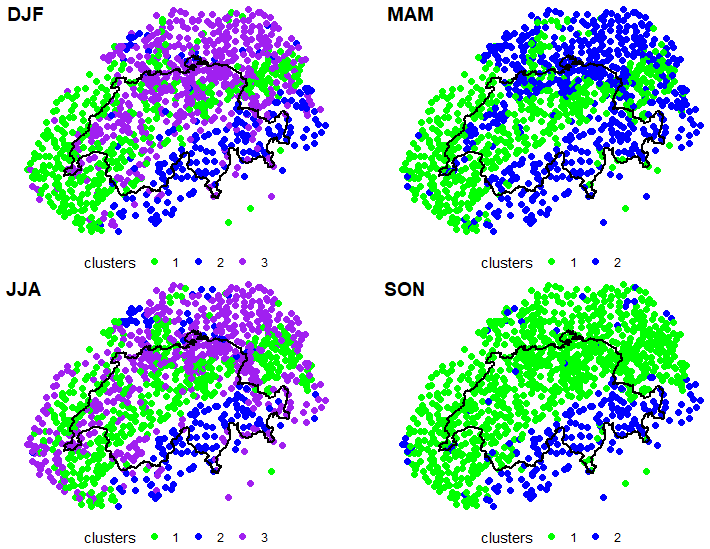
Figure 2 Maps of Switzerland showing the optimal number of clusters identified with the PAM algorithm for each season. For each season, the regions identified are color-coded. From top left, going clockwise, DJF (two clusters), MAM (two clusters), JJA (three clusters) and SON (three clusters).

5 Results

5.1 Estimated regions with RFA by upper-tail behavior

Figure 2 shows the optimal number of clusters identified for each season. We have three clusters in the case of winter (DJF), two in spring (MAM), three in summer (JJA), and two in fall (SON). Notably, although the spatial coordinates are not used, the identified clusters are somehow spatially plausible for each season. Stations in the south are generally in the same cluster. In the north, the stations located in the northern rim and the Jura generally fall in the same cluster. This is partly according to our knowledge of the spatial pattern of heavy precipitation in the respective seasons. A few stations for each season, however, appeared in clusters different from their neighbors.

5.2 Estimated regions with the ROI method

Figure 3 presents the neighborhoods found for each station. In panel a is the map of Switzerland showing the stations with the size corresponding to the size of the radius identified and the color indicating a local fit will be done (for stations without any neighbors) or a regional fit (for stations with at least one neighbor). For those without neighbors, the search sometimes terminated at a very small distance. This means that, although they have proximate neighbors according to the crossing distance, the homogeneity test failed. For some stations, however, no neighbors are found. These are stations whose closest neighbors are at large crossing distances, and the test failed after application.

In Fig. 3b, the histogram of the neighborhood size, as well as the average number of neighbors identified for each class, is shown. Only a few stations reach the bound of 100 km. The observed seasonal differences are due to the seasonality and spatial variability of daily precipitation in Switzerland. We recall that the identification of the regions for each station is based on the homogeneity of the scaled extremes. The occurrence of these extremes and their quantity, which affects the test of homogeneity (Evin et al., 2016), depends on the season and hence the observed seasonal differences.

In our subsequent experiments, we keep these neighborhoods and fit accordingly the model versions described in Sects. 3.3.2 and 3.3.3, i.e., ROI_EGPD_Full and ROI_EGPD_Semi. For all the stations without any neighborhood, we simply fit a local EGPD model.

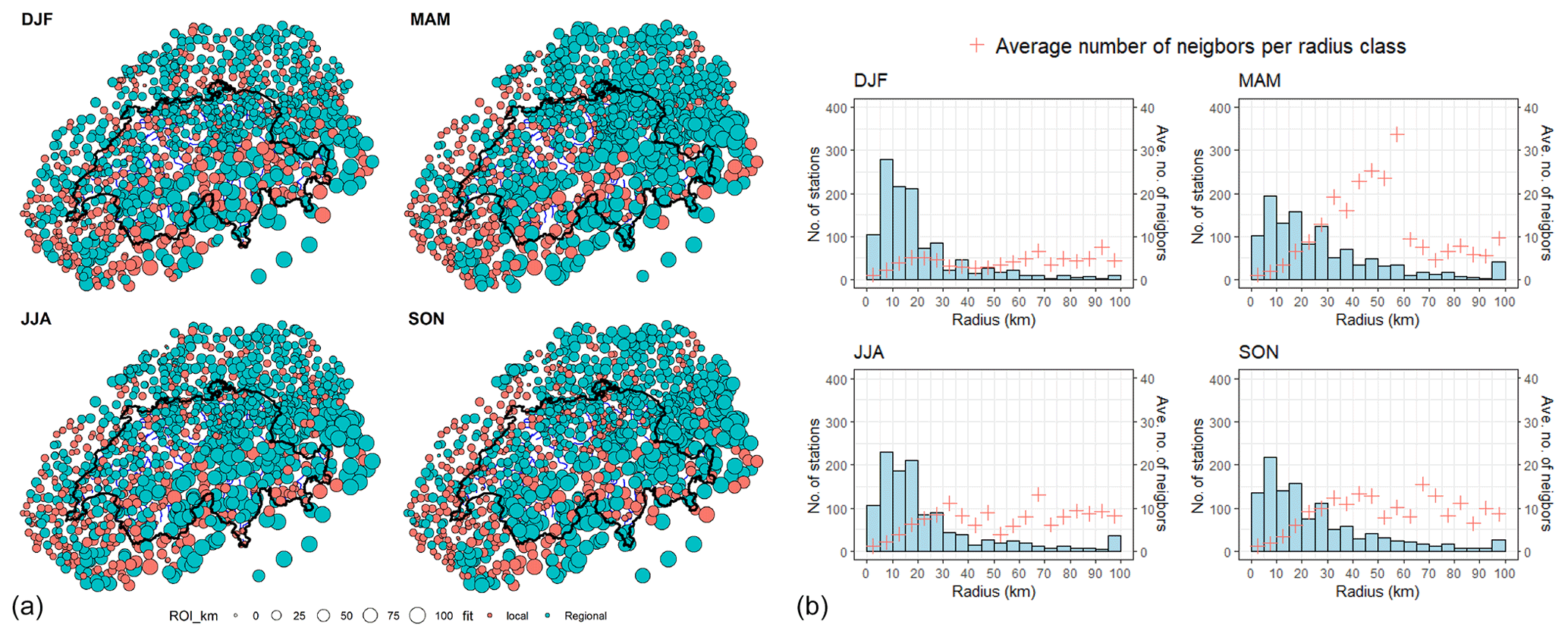
Figure 3 Properties of the ROI identified for each station. (a) Seasonal maps showing the size of the ROI per station. For each season, the size of the circle is proportional to the ROI size: the smallest is 0 (km), and the largest is 100 (km). The color of the circle indicates whether a local fit is done or a regional fit. (b) Histogram of the size of the ROI identified. The red points indicate the average number of neighbors identified for each ROI class.

5.3 Choice of covariates in the GAM

Following the outlined methodology for the spatial model in Sect. 3.2.3, we present in this part the choice of covariate combinations made for the EGPD model.

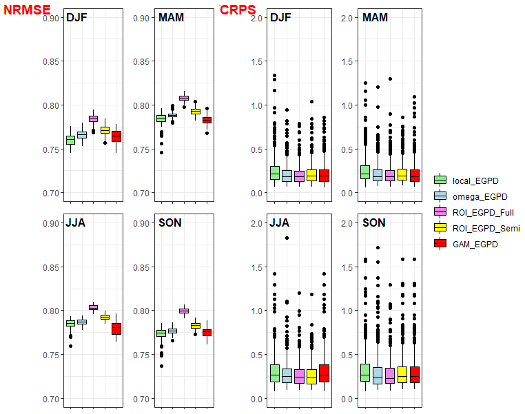
Figure 4 Criteria applied to the bulk of the distribution for each season. Left: accuracy of the whole distribution as measured by the NRMSE; each box plot contains 100 values. Right: CRPS score; each box plot contains 500 points, 1 per station.

We use longitude, latitude, and the mean daily precipitation to explain the parameters of EGPD, that is, k, σ, and ξ. Other covariates would be possible, but we use these ones because they are readily available, and so estimation at ungauged locations would be possible. After testing different combinations of the covariates, we use the following forms for the relationships

$$\begin{array}{}\text{(13)}& {\displaystyle }k=s\left(m\right),\text{(14)}& {\displaystyle }\mathit{\sigma }=s(\text{lon},\text{lat})+s\left(m\right),\text{(15)}& {\displaystyle }\mathit{\xi }=s(\text{lon},\text{lat}),\end{array}$$

where s(lon,lat) means a thin plate spline smooth s on the longitude lon and latitude lat, and s(m) means a cubic spline on the mean daily precipitation (m).

Although all three model parameters have to be positive, we still used the identity link function to reduce the complexity in the generation of the gradients of the negative likelihood function of the EGPD model (necessary for model fitting in GAM; see Wood et al., 2016). We, however, imposed constraints on the likelihood function to ensure that the parameters remain positive.

5.4 Model comparison

In this section, we present the results of the comparison between the competing models, as judged by the criteria introduced in Sect. 4. We remind the reader that the sampling was repeated 50 times for all the models, and so, for clarity, we show the box plots of the criteria. Each box plot contains 50 values of the criteria obtained per run in the case of SPAN, 100 in the case of FF and NRMSE, and 500 in the case of CRPS (500 corresponds to the number of stations in Switzerland which the criteria were computed on).

First, the accuracy/reliability of the models in the bulk of the distribution as measured by the NRMSE is shown on the left of Fig. 4. The results are shown per season, and the closer the value is to 1, the more accurate the model is. From this result we can clearly see that, for all seasons, the two models based on ROI are the most reliable. The ROI_EGPD_Full model (where we regionalize according to the ROI method, all three parameters of the EGPD model) is the best model compared to ROI_EGPD_Semi model 4 (where only the shape parameter is regionalized but the other two parameters are locally estimated). The performance of the other regional models is similar, and there is no large improvement in these models over the local EGPD model according to these criteria.

The CRPS score gives a combined measure of the spread and reliability of the competing models. A model should not only assign the correct probabilities to the observations, but the spread of the probabilities estimated from the different sub-samples (100 in our case) should also be low as well. We computed this score for all the positive observations at every station. The best model should have the smallest score.

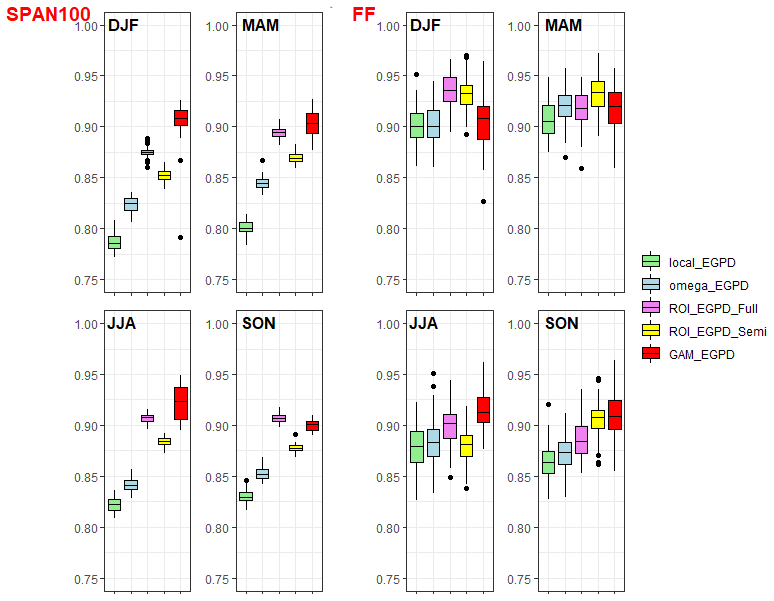
Figure 5 Criteria applied to the upper tail for each season. Left: robustness of the local EGPD and the four candidate models, as measured by the SPAN criteria. The stability is measured with respect to a 100-year return-level estimate. Each box plot contains 50 values. Right: reliability in prediction of the maxima as measured by the FF criteria; each box plot contains 100 values.

The plot on the right of Fig. 4 presents the seasonal box plots for the CRPS of the five models. Each box plot consists of 500 points, 1 per station (recall the scores are computed for only the 500 stations located within Switzerland). From the box plots and the medians, it is clear that ROI_EGPD_Full has the smallest value of this score. For all seasons (except summer), the local model has the largest score, showing that the models offer improvement over the local model.

The stability/robustness of the estimate of a 100-year return level in between two periods as measured by the SPAN criteria is shown on the left of Fig. 5. Obviously, all the regional models show clear improvement in robustness over the local EGPD model. The spatial model (GAM_EGPD) shows the highest robustness over all the models, except in fall, when it is slightly overtaken by the ROI_EGPD_Full model. The results also show that, of all four regional models, the RFA model based on the upper tail (Omega_EGPD) has the smallest robustness. In the case of the two ROI models, ROI_EGPD_Full is more robust compared to the ROI_EGPD_Semi model. The former involves regionalizing all three model parameters, while the latter involves only the shape parameter regionalization. Looking at the two models where only the shape parameter is regionalized, the model based on ROI (ROI_EGPD_Semi) is more robust in all the seasons compared to the model based on upper-tail behavior that involves clustering (Omega_EGPD).

Finally, the FF score measures the reliability of the models in the upper tail, more precisely in the prediction of the maximum observed value. This criterion is also optimized at a value of 1. The plot on the right of Fig. 5 shows generally high values of this score for all the models, indicating that they are generally reliable in the prediction of the maximum observed value. For all the seasons, all the regional models appear to be more reliable compared to the local model. An exception is however in the case of Omega_EGPD in winter and ROI_EGPD_Semi in summer (looking at the median). In fall and summer, the GAM_EGPD model emerges as the most reliable. While in winter ROI_EGPD_Full is the most reliable, ROI_EGPD_Semi is the most reliable in spring.

Table 2 Summary of the comparison results from the four criteria used. For each season and criterion, the model with the highest median is shown. In the case of the CRPS score, however, the model with the smallest median CRPS is shown.

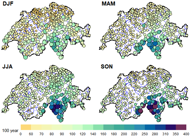
Figure 6 Map of Switzerland showing the 100-year return level for the four seasons as predicted with the ROI_EGPD_Full model.

To conclude, we present an overall summary of the results in Table 2 by focusing on the median of the box plots. We also show the map of the seasonal 100-year return level predicted with the ROI_EGPD_Full model in Fig. 6. The maps reveal a clear seasonality and spatial pattern. Ticino in the south is subject to the highest levels, especially in the fall, where up to 400 mm can be expected.

6 Conclusions and discussion

The objective of this contribution was to compare three methods to improve the at-site estimates of daily precipitation. By considering a dense network of 1176 stations mainly located in Switzerland, we compared methods based on different philosophies to regionalize the estimation of daily precipitation. The first method defines homogeneous regions based on their upper-tail similarity. No covariate is used in the delineation of regions, but only the precipitation data at hand. The second method avoids defining “hard” clusters but assumes that every station has its homogeneous region that can be identified using homogeneity tests. The third method is spatially based, so all the data are used to estimate smooth and flexible surfaces for the model parameters. Pooling the data to estimate the surfaces thus ensures sharing of information between stations. Using these methods, we built four regional EGPD models and compared them. The comparison is based on the accuracy, robustness, and reliability of the models in a cross-validation framework. More precisely, we assessed the performance in both the bulk of the distribution (NRMSE and CRPS) and the upper tail (SPAN and FF).

In contrast to most comparative studies of regionalization approaches that focused on extreme distributions (GEV or POT), we assumed the daily data to follow the EGPD. This distribution can adequately model the full spectrum of precipitation intensities. It has the elegant property of being EVT compliant in both the upper and lower tails while providing for a smooth transition in between.

The results showed that regionalization offers improvement in robustness and reliability even in the case of a full-scale model (EGPD) that includes all the data in the estimation of its parameters.

From the four criteria used, the performance depends on the season, but we can still draw the following conclusions.

• In terms of the reliability/accuracy over the whole distribution, the ROI model (ROI_EGPD_Full), with all parameters regionalized, emerged as the most accurate.

• Reliability in the prediction of the maxima, as measured by FF, indicated that the GAM is the most reliable, especially in the seasons with the heaviest rainfall (summer and fall).

• The GAM emerged as the most robust (SPAN) and is followed closely by the ROI model (ROI_EGPD_Full).

In conclusion, two models compete hand in hand: the ROI model (ROI_EGPD_Full) and the GAM. When we focus on the bulk of the distribution (NRMSE and CRPS), ROI_EGPD_Full is the best model. When we however focus on the far tail (FF and SPAN), the GAM is the best. As Garavaglia et al. (2011) pointed out, the two properties of reliability and robustness are complementary. For two models of similar reliability, the model with the best robustness should be preferred. Given this, the GAM on EGPD, combining both properties in the upper tail, can be said to be the preferred method. We note, however, a major drawback of the GAM. It requires significant computational time as compared to the ROI, especially in our case, where we have a dense network (1176 stations) with long series (up to 156 years for some stations), and we use all the positive precipitation. In practice, thus, it would be much easier to use ROI compared to the GAM, given that the performance of both is similar and the former is more reliable when we consider the whole distribution (a feature of interest in our case), not only maxima.

It is worth noting that, in the course of the present study, we focused our evaluation at the station level, where we have observations. A further step will be to assess the models more generally by looking at their performance at ungauged locations in spatial cross-validation as done by Blanchet and Lehning (2010), Carreau et al. (2013) or more generally the framework proposed by Blanchet et al. (2019). In this respect, the spatial model based on the GAM offers a key advantage over the other methods since it inherently results in a regional model that can be applied everywhere. In the case of the other methods, however, the step of choosing the appropriate interpolation technique has to be considered. It is also worth mentioning the inherent drawback of conventional RFA approaches involving “hard” clustering, in this case the Omega_EGPD model. They are known to produce abrupt parameter shifts (in our case, the shape parameter) along the boundaries of the contiguous regions. Again, estimation at ungauged locations between two homogeneous regions with a significant difference in the regional shape parameter will be a difficult decision. The method of ROI however circumvents some of the drawbacks of the conventional RFA approach.

Finally, our approach also assumed the spatial independence of the observations. This assumption will however not be true, especially since we have considered all the positive precipitation. We however expect the benefit of the regional approach to outweigh the consequences of ignoring the spatial dependence (Hosking and Wallis, 1988), especially since our interest is in the marginal distribution only (Zheng et al., 2015). An interesting aspect is also to improve the method based on omega (see 3.2.1) to take into account both the margins and the dependence between sites.