the Creative Commons Attribution 4.0 License.
the Creative Commons Attribution 4.0 License.
 | 23 May 2022
Hydrometeorological evaluation of two nowcasting systems for Mediterranean heavy precipitation events with operational considerations
Alexane Lovat
Béatrice Vincendon
Véronique Ducrocq
Heavy precipitation events and subsequent flash floods regularly affect the Mediterranean coastal regions. In these situations, forecasting rainfall and river discharges is crucial especially up to 6 h, which is a relevant lead time for emergency services in times of crisis. The present study investigates the hydrometeorological skills of two new nowcasting systems: a numerical weather model AROME-NWC and a nowcasting system blending numerical weather prediction and extrapolation of radar estimation called PIAF. Their performance is assessed for 10 past heavy precipitation events that occurred in southeastern France. Precipitation forecasts are evaluated at a 15- min time resolution and the availability times of forecasts, based on the operational Météo-France suites, are taken into account when performing the evaluation. Rainfall observations and forecasts were first compared using a point-to-point approach. Then the evaluation was conducted from an hydrological point of view, by comparing observed and forecast precipitation over watersheds affected by floods. In general, the results led to the same conclusions for both evaluations. On the very first lead times, up to 1 h 15 min and 1 h 30 min of forecast, the performance of PIAF was higher than AROME-NWC. For longer lead times (up to 3 h) their performances were generally equivalent. An assessment of river discharges simulated with the ISBA-TOP coupled system, which is dedicated to Mediterranean flash flood simulations and driven by AROME-NWC and PIAF rainfall forecasts, was also performed on two exceptional past flash flood events. The results obtained for these two events show that using AROME-NWC or PIAF rainfall forecasts is promising for flash flood forecasting in terms of peak intensity, timing, and first wave of discharge, with an anticipation of these phenomena that can reach several hours.
- Article
(5407 KB) - Full-text XML
- BibTeX
- EndNote


The Mediterranean coastal regions are frequently affected by heavy precipitation events (Ricard et al., 2012). The mesoscale convective systems associated with these events produce a large amount of rainfall, typically greater than 100 or 200 mm in only a few hours. The occurrence of such intense rainfall over small areas and catchments up to a few hundreds of square kilometres often trigger devastating flash floods. These events threaten people as well as property (Drobinski et al., 2014; Gaume et al., 2016) and result in direct economic losses valued at hundreds of millions of euros each year. Even if significant progress has been realized in the last decades, very localized and high-intensity rainfall events, such as those generated with the Mediterranean precipitating systems are difficult to forecast (Alfieri et al., 2012; Vié, 2012; Silvestro et al., 2017). It is difficult to forecast heavy precipitation events with accurate intensity, chronology and location. Among the difficulties encountered are the complex features and variability of deep convection and the associated small spatiotemporal scales that are hardly predictable. Nowcasting systems suit these scales with high spatial and temporal resolution of short-term forecasts (usually up to a few hours). They can be based on extrapolation of observations or rely on mesoscale numerical weather prediction or combine these two approaches. The concept of extrapolation of radar echoes for short-term precipitation forecasting was first developed in 1953 (Ligda, 1953). This approach has been deepened by the search for fast-computing algorithms or methods allowing the best forecasts of the evolution of precipitating cells (in terms of displacement, size and intensity) from the radar imagery data. Among them there are those based on cross-correlation (e.g. Rinehart and Garvey, 1978) and those based on individual radar echo tracking (Johnson et al., 1998; Dixon and Wiener, 1993). These methods were later improved to ensure the consistency of the velocity field reconstructed after extrapolation (Li et al., 1995; Laroche and Zawadzki, 1995; Germann and Zawadzki, 2004). Although widely used, the accuracy of extrapolation methods is limited because they are not able to forecast convective storm initiation, growth and decay (Golding, 1998). Beyond 1 or 2 h, the use of numerical weather prediction is necessary to depict rapidly changing conditions. The latest generation of mesoscale models enables kilometre horizontal resolutions to be achieved and is able to reproduce fine-scale boundary layer and convection processes. Numerical weather prediction systems have been configured to meet the requirements of nowcasting, i.e. to have very short-term forecasts, updated with the latest observations in the fastest possible time. These systems are based on the same kilometre horizontal resolution models as the forecast models used for forecasting the weather over the next 24–48 h, but their assimilation frequency and windows are adapted to allow the forecasts to be frequently refreshed with new observations while ensuring short forecast delivery times (Weygandt et al., 2009). The AROME-NWC (Auger et al., 2015), which is a system operationally used at the French meteorological service Météo-France, is one of them. Thus, several nowcasting system types with various skills coexist at lead times between 1 and 3–4 h. Methods have been developed to combine extrapolation methods and numerical prediction systems. Seamless forecasts can be obtained by weighting precipitation fields from radar extrapolation and numerical weather prediction forecasts. The first approach in blending nowcasting was introduced by Golding (1998) with a heavy weighting for the extrapolation nowcasting during the first hour and a heavier weighting transitioning to the numerical forecasts with increasing lead time. A new nowcasting system called PIAF (Moisselin et al., 2019) blending numerical weather prediction and extrapolation of radar estimation has recently been developed by the nowcasting department at Météo-France. Its skills for rainfall forecasting still need to be assessed.
The short hydrological response times ranging from few minutes to few hours after heavy downpours are a major issue for notifying at-risk populations and planning the intervention of emergency services in times of crisis. The use of rainfall nowcasting allows the lead time of hydrological forecasts to be extended by a few hours compared to the mere use of observed precipitation data that limit the forecast lead time by the catchment response time. Vivoni et al. (2006), Berenguer et al. (2005) and Dolcine et al. (2001) have demonstrated the benefit of using deterministic rainfall forecasts obtained from radar-based extrapolation as input to hydrological models. Other studies explored the potential of probabilistic rainfall nowcasting for flash flood forecasting (Silvestro and Rebora, 2012; Poletti et al., 2019). Nowcasting flash floods provides an anticipation time sufficient enough to boost the preparedness of people and civil protection and sometimes a valuable time to prevent the authorities from being completely unprepared for the occurring or upcoming event (Silvestro et al., 2017). The availability time of the rainfall forecast is thus crucial for real-time streamflow forecasting. Whereas operational hydrological models are often fast-running (i.e. finishing in seconds to minutes) weather forecasts require more time to be delivered. Therefore, this delay is taken into account in this study to consider the operational real-time constraints.
The present study investigates the hydrometeorological skills of AROME-NWC (Auger et al., 2015) and PIAF (Moisselin et al., 2019), two new nowcasting systems operationally used at the French meteorological service Météo-France. The main objectives are to compare and evaluate their performance for 10 past Mediterranean heavy precipitation events and to suggest some best practices for real-time forecasting. The effect of spatial resolution, lead time and precipitation intensity on forecasting skill is studied at a 15- min time resolution. Precipitation forecasts are first evaluated from a meteorological perspective with a synoptic scale verification using a point-to-point approach. Rainfall observations and forecasts are compared at each grid point of an area covering southeastern France. Then an evaluation on scales relevant to hydrology is performed by comparing observed and forecast rainfall averaged over watersheds affected by past floods. An assessment of river discharges simulated with ISBA-TOP, a model dedicated to Mediterranean flash flood simulations (Bouilloud et al., 2010; Vincendon et al., 2016), driven by AROME-NWC and PIAF rainfall forecasts was also conducted on two French exceptional recent flash flood events. The performance of the forecasts is assessed in terms of intensity and timing of the flood peak.
This paper is organized as follows. Section 2 describes the case studies, the nowcasting systems, the hydrological system, and the verification methods. The results of the different verifications are presented and discussed in Sect. 3. The conclusions are reported in Sect. 4.
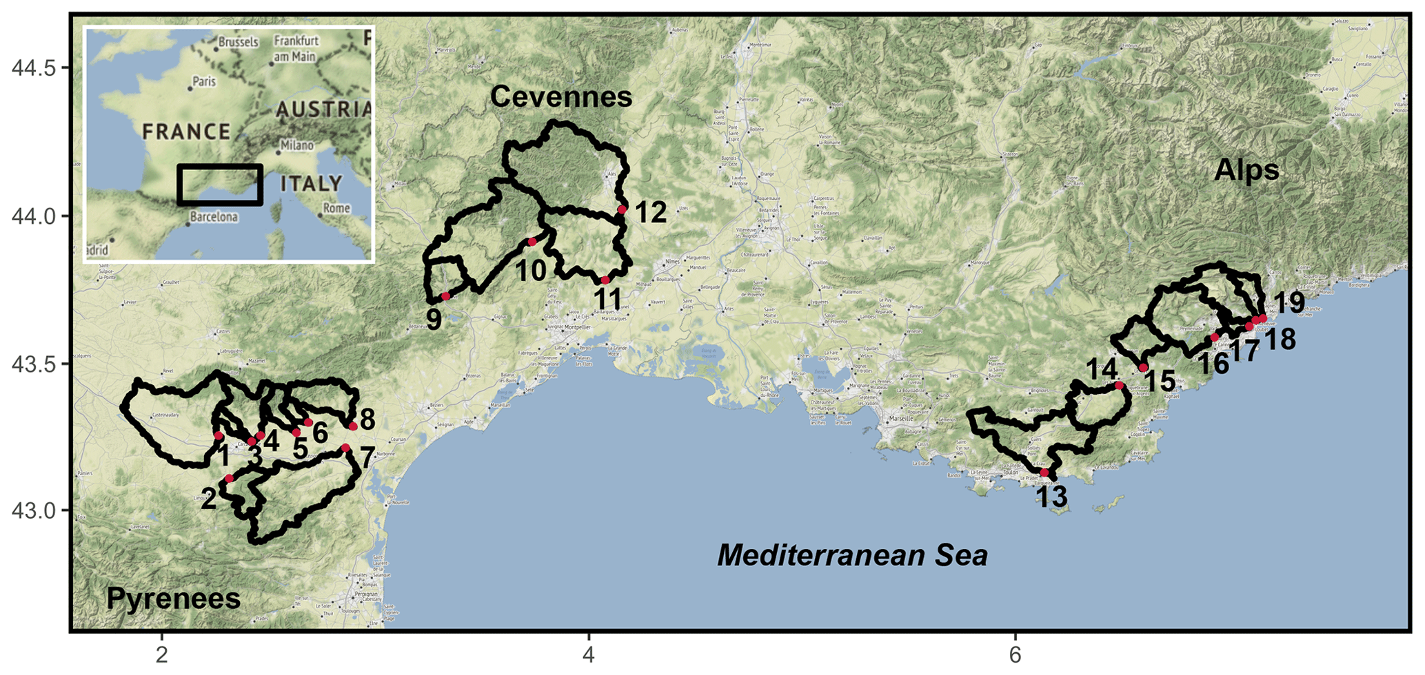
Figure 1The black rectangle indicates the study area in France. The thick lines delineate the studied watersheds within this zone. The red circles correspond to the associated outlets. The base map used in the background was plotted in R with ggmap (Kahle and Wickham, 2013) and © Stamen Maps.
2.1 Case studies
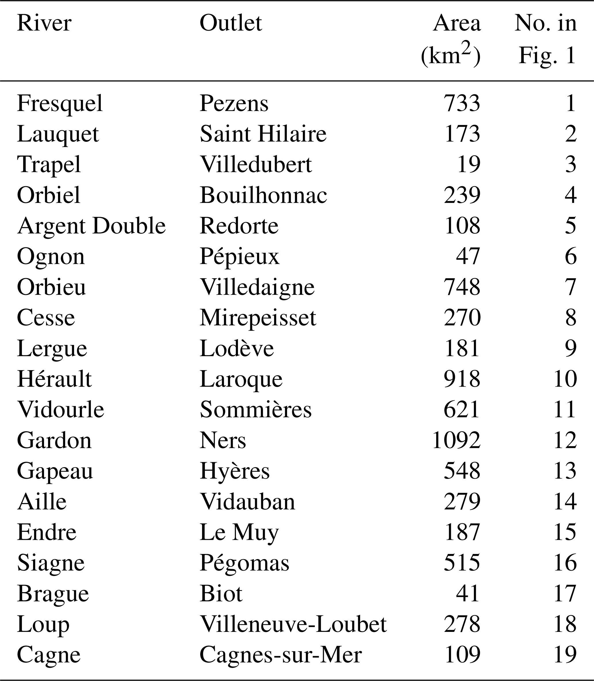
The selected case studies concern recent heavy precipitation events which occurred in Southeast France between October 2015 and November 2018. A rectangular verification zone was defined to investigate the performance of the nowcasting systems during these events. It encompasses the regions along the Mediterranean coast most favourable to intense events (black rectangle in Fig. 1) such as the eastern Pyrenees, the southern Alps, and the Cévennes-Vivarais region. This area is characterized by a pronounced topography with steep slopes and narrow valleys. Within this large zone (110 000 km2), 19 catchments with areas ranging from 19 to 1100 km2 and short response times were selected for the hydrological evaluation (Table 1). Watersheds numbered 1–8 in Fig. 1 are all tributaries of the Aude river in the northeast of the Pyrenees. Watersheds numbered 9–12 are located in the Cévennes region. The other watersheds numbered 13–19 are located in the French Riviera.
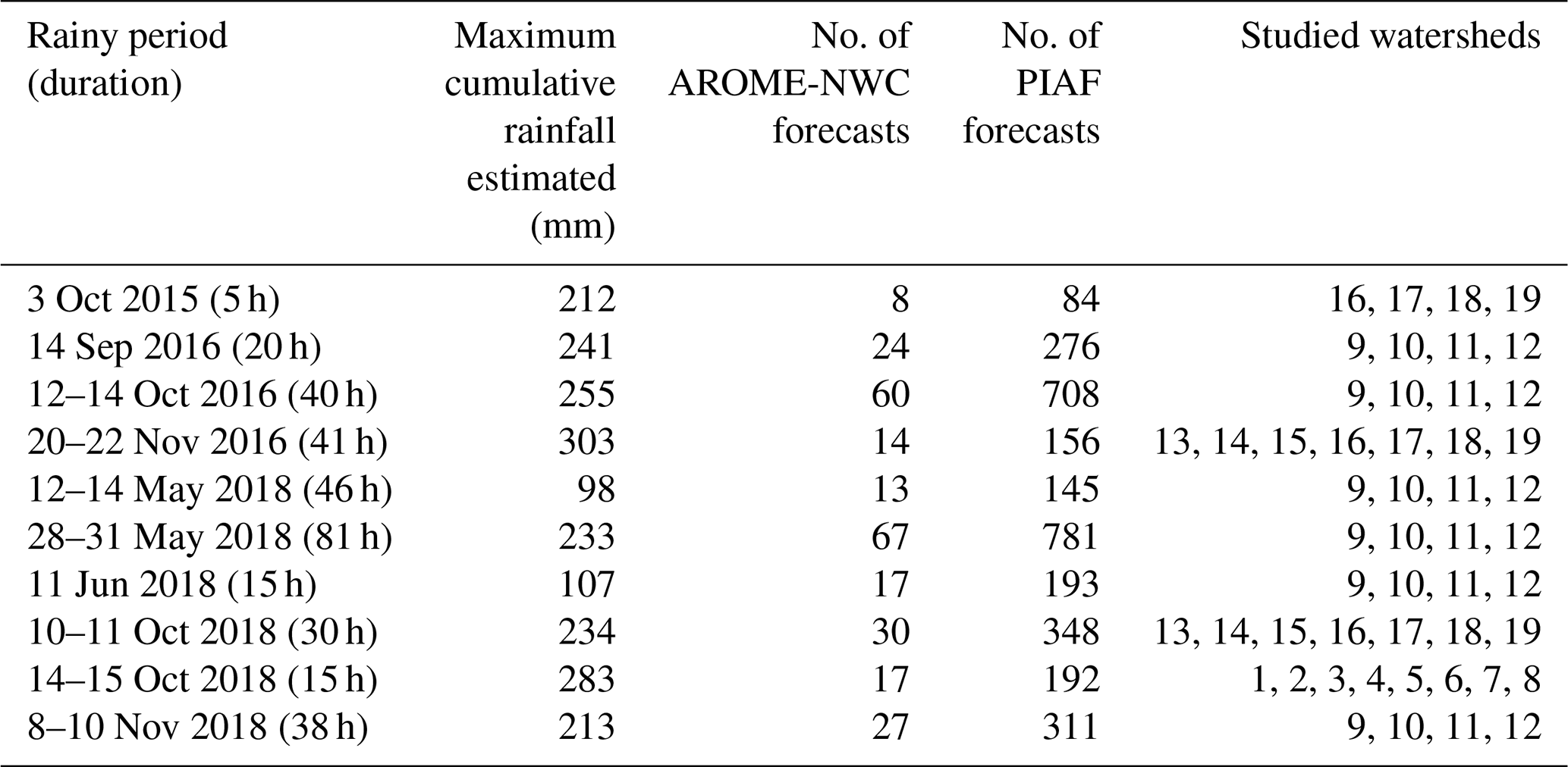
To assess the performance of the nowcasting systems, 10 recent heavy precipitation events were considered (first and second columns of Table 2). These rainy episodes are representative of the variety of rainfall intensities and durations and the hydrological responses of the rivers encountered in the French Mediterranean coastal regions. In particular, the two events that occurred on 3 October 2015 in the French Riviera and 14–15 October 2018 in the Aude region are among the latest major tragic flash flood events that have affected metropolitan France. They represent together 34 deaths and more than Euro 800 million of damage. More details about the October 2015 event and the October 2018 event were given by Payrastre et al. (2016) and Caumont et al. (2020), respectively.
Table 2Characteristics of the studied events and number of forecasts. Quantitative precipitation estimates come from ANTILOPE product.
2.2 The nowcasting systems
2.2.1 AROME-NWC
The AROME-NWC (Auger et al., 2015) is a configuration of the French numerical weather prediction system AROME-France (Seity et al., 2011; Brousseau et al., 2016) especially designed for nowcasting purposes. The AROME-NWC is a mesoscale and non-hydrostatic model. Its horizontal resolution is 1.3 km × 1.3 km and its vertical grid has 90 levels ranging from 10 to around 30 000 m above the ground. The deep convection is explicitly resolved and the microphysical processes are governed by the ICE3 one‐moment bulk microphysical scheme (Pinty and Jabouille, 1998). The AROME-NWC is thus able to forecast mesoscale convective systems that caused heavy rain in the Mediterranean area. Boundary conditions are provided by the analysis of the ARPEGE global operational numerical weather prediction model. The AROME NWC initial conditions are provided by a three-dimensional variational (3D-Var) data assimilation of observations available within 20 min windows centred on the analysis time, each hour. The observations are primarily radar (reflectivity and radial velocity) data, screen level measurements, and to a lesser extent, aircraft, sounding and satellite data. The AROME-NWC is run every hour and provides short-range forecasts up to 6 h with a time step of 15 min on a domain covering France and adjacent areas. Forecasts were available within 35 min at the time of the study.
2.2.2 PIAF
Very recently the nowcasting department of Météo-France has developed a new nowcasting system PIAF (for “Prévision Immédiate Agrégée Fusionnée” in French, Moisselin et al., 2019), which is a data fusion product between radar extrapolation and numerical prediction (the rainfall forecast by AROME-NWC). For the extrapolation of radar quantitative precipitation estimations radar data are processed as follows: rainy cells are identified by windows surrounding areas of connected pixels above a given threshold, the displacement of each cell is determined using the previous image (highest correlation), a gridded motion field is computed from the movement vectors of the cells with different threshold values and applied to the cells to extrapolate them in the future.
The PIAF is based on a sequential aggregation of these two predictors (radar extrapolation and numerical prediction) and the result of blending is a linear compound of both of the form: PIAF = α × Extrapolation + (1−α) × AROME-NWC. Its aim is to perform better than the best predictor. The accuracy of a prediction proposed by the experts (radar extrapolation and AROME-NWC) or by PIAF is measured through a loss function. The Gerrity score (Gerrity, 1992) described in Appendix A is used here to estimate the loss of each product with respect to the radar quantitative precipitation estimates. The difference between the forecaster accumulated loss and that of an expert is called regret, as it measures how much the forecaster regrets, in hindsight, not having followed the advice of this particular expert (Cesa-Bianchi and Lugosi, 2006). As the forecaster’s goal is to minimize the regret, the weights given to each predictor in PIAF are adjusted according to their deviation from the previous 6 h observations, this results in more weighting of the expert whose cumulative loss is small. The polynomially weighted average forecaster with multiple learning rates (ML-Poly, Cesa-Bianchi and Lugosi, 2006; Gaillard and Goude, 2015) is the aggregation rule used in PIAF to assign weights to each predictor. This method provides a real choice of predictor rather than a mixture. The weights depend also on the forecast range (Fig. 2) and on the geographical area according to a division of France into six sub-areas. The PIAF is run every 5 min with a 3 h lead time and a time step of 5 min. Forecasts are available within 2 min.
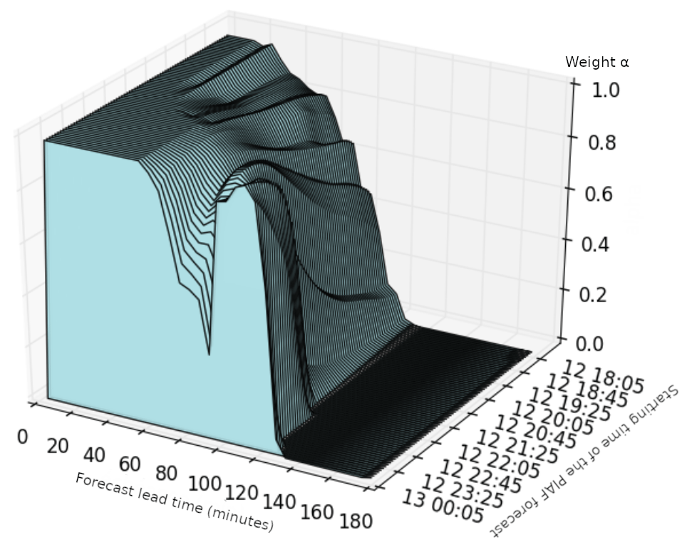
Figure 23-D representation of the weight α given to radar extrapolation in PIAF. It shows the PIAF forecast lead time (interval [0, 180 min]) dependency on α (interval [0, 1]) for PIAF forecasts starting from 12 October 2016 18:05 coordinated universal time (UTC) to 13 October 2016 00:05 UTC.
2.3 The hydrometeorological model ISBA-TOP
The ISBA-TOP (Bouilloud et al., 2010; Vincendon et al., 2016) is a distributed model designed to simulate the hydrological response of Mediterranean catchments during heavy precipitation events. It is based on the coupling between the land surface model ISBA (Interaction Surface Biosphere Atmosphere, Noilhan and Planton, 1989) and TOPODYN (Pellarin et al., 2002), a variant dedicated to flash flood modelling of the hydrological model TOPMODEL (Beven and Kirkby, 1979). This coupling consists of introducing into ISBA a lateral distribution of soil water following the TOPODYN concept. The ISBA deals with the water and energy budgets within the soil column and between the vegetation and the atmosphere above. Fluxes are computed for all grid meshes of its domain. From the resulting volumetric water content over a ISBA grid cell, water storage deficit as well as the hill slope recharge are determined on the corresponding TOPODYN watershed pixels of 50 m × 50 m resolution. TOPODYN manages the computation of the lateral redistribution of water within the catchment by using topographical indexes and the spatial variability of the rainfall. The new saturated areas and new soil moisture fields obtained by TOPODYN are then aggregated on the ISBA mesh to update water contents in ISBA. From them, ISBA computes sub-surface runoff and deep drainage which are dispatched on each 50m-sided pixel and then routed up to the river and total discharges are then produced at catchment outlets.
The ISBA-TOP configuration used in this study is the one suggested by Lovat et al. (2019) for flash-flood simulations, based on SRTM data for orography, Land use/cover area frame statistical survey topsoil data (Ballabio et al., 2016) for soil texture, ECOCLIMAP-II (Masson et al., 2003; Faroux et al., 2013) data for land cover, and a spatial resolution of 300 m for ISBA.
The ISBA-TOP coupled system has been run during the HyMex special observing periods for real-time prediction of discharges for watersheds in the Cévennes-Vivarais region and the Mediterranean coastline of southeastern France. Its performance was also assessed for Italian watersheds (Nuissier et al., 2016). ISBA-TOP is used in operations in the National Institute of Meteorology and Hydrology of Bulgaria for the Arda river flood forecasting (Artinyan et al., 2016). In addition to simulating river discharges during flash floods, ISBA-TOP is also able to simulate intense runoff phenomena (Vincendon et al., 2016; Lovat et al., 2019).
2.4 Verification methods
To evaluate the quality of the precipitation forecast provided by AROME-NWC and PIAF, the 1 km2 quantitative precipitation estimates ANTILOPE (Laurantin, 2008) at a 15 min time resolution, in which merged observations from the Météo-France radar and the rain gauge network were used as reference data and are called observed data or observation hereafter. Two verification methods were applied for the rainfall nowcasting evaluation process. The first method, commonly used in the meteorological community, was based on point-to-point comparisons of the forecasts and observations. Comparisons were performed at each grid point of a common 1 km resolution grid over a large area of 110 000 km2 covering southeastern France (see the black rectangle of the Fig. 1). The rainfall fields were downscaled over the common grid by using a nearest grid point interpolation method. The second evaluation was carried out from a hydrological point of view by comparing observed and forecast rainfall averaged over the surface of watersheds affected by floods. For both evaluations, the available forecasts covering 10 recent heavy precipitation events occurring in southeastern France between 2015 and 2018 were considered (Table 2).
The observations and forecasts used in this study have different time resolutions (15 min for ANTILOPE and AROME-NWC, and 5 min for PIAF). The comparisons have been carried out by using a common accumulation time step of 15 min. This time step allows characterization of the high rainfall temporal variability, notably for convective situations.
One original feature of this study is that the availability times of forecasts, based on the operational Météo-France suites, are taken into account when performing the evaluation. Forecasts are released with a time delay of 35 min for AROME-NWC and of 2 min for PIAF. To coincide and easily compare observations and forecasts over full 15 min time intervals, the first 45 min of the AROME-NWC forecast are not considered for the evaluation. Similarly, the first 5, 10 or 15 min of the PIAF forecast are not used in the evaluation (Fig. 3). As PIAF forecasts last 180 min and AROME-NWC forecasts last 360 min, they are not evaluated in the same time window. Their performance can be compared only at lead times less than 180 min.
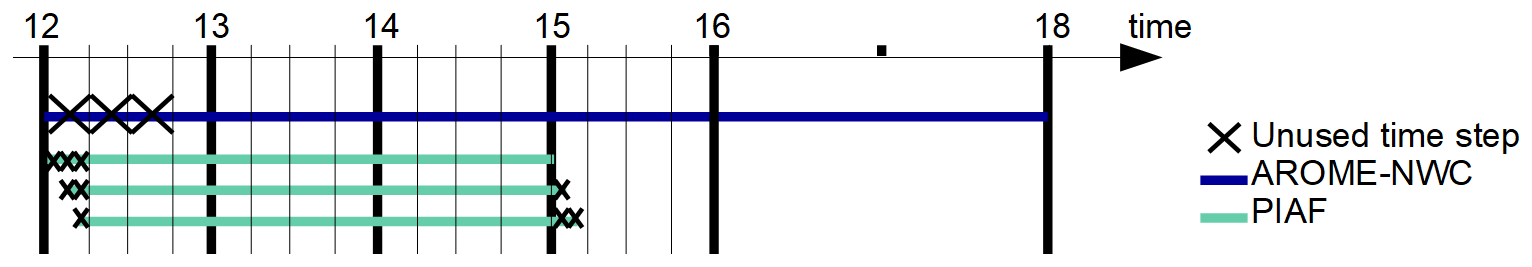
Figure 3Example showing the unused time steps for a AROME-NWC forecast run starting at 12:00 UTC and for three successive PIAF forecasts starting at 12:00, 12:05 and 12:10 UTC.
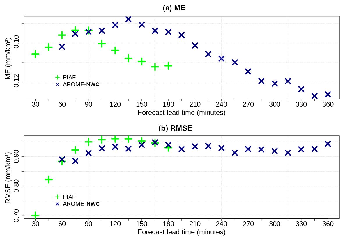
Figure 4(a) Mean and (b) root mean square errors for AROME-NWC (in blue) and PIAF (in green) over their respective forecast ranges for 15 min rain accumulation forecasts. Scores computed over the box displayed in Fig. 1.
Even if watershed integration allows evaluation of quantitative precipitation forecasts over given surfaces, it does not allow evaluation of whether rainfall amounts occur at the right location with the right chronology within the catchments. An assessment of AROME-NWC and PIAF performance for flash flood nowcasting was also performed through running of hydrological forecasts using ISBA-TOP for two events that occurred on 3 October 2015 and on 14–15 October 2018. The reference is the discharge simulation obtained using the radar rainfall estimates ANTILOPE as input to the distributed hydrological model. This approach allows dissociation of the error made by the hydrological model from that made by the rainfall forecasts (Borga, 2002; Berenguer et al., 2005; Poletti et al., 2019). Initial conditions (surface soil water and temperature) come from the Météo‐France hydrometeorological operational system SAFRAN‐ISBA‐MODCOU (Habets et al., 1999). ISBA-TOP, which needs calibration for its routing parameters, was calibrated as described by Bouilloud et al. (2010) for hourly rainfall estimates, thus only hourly discharges were simulated. These hydrological simulations systematically stop at the end time of the rainfall forecast, even if the basin concentration time would make it possible to extend the hydrological forecast beyond the rainfall forecast horizon.
3.1 Point-to-point evaluation of the rainfall nowcasting
The results of the evaluation are presented for AROME-NWC and PIAF separately before comparing both systems. Scores used here are described in Appendix A.
The mean and root mean square errors are shown as a function of lead time in Fig. 4 for 15 min rain accumulation forecasts. In general the AROME-NWC root mean square error increases slightly with lead time. The mean error resulting from the difference between forecasts and observations is negative indicating that precipitations are underestimated by the model on average. Four standard categorical verification scores are presented in Fig. 5 to summarize the performance of 15 min rain accumulation forecasts from AROME-NWC and PIAF. These are the hit rate, the false alarm rate, the Heidke skill score (HSS) and the frequency bias as functions of lead time for two thresholds characterizing precipitation occurrence and more intense precipitation: 0.5 mm/15 min and 3 mm/15 min. The hit rate and HSS slightly decrease with increasing lead time. The false alarm rate of AROME-NWC depends little on the forecast lead time regardless of the threshold. For the higher rainfall intensities (3 mm/15 min) the frequency bias is greater than 1, indicating a trend to predict these rainfall accumulations too frequently at all lead times.
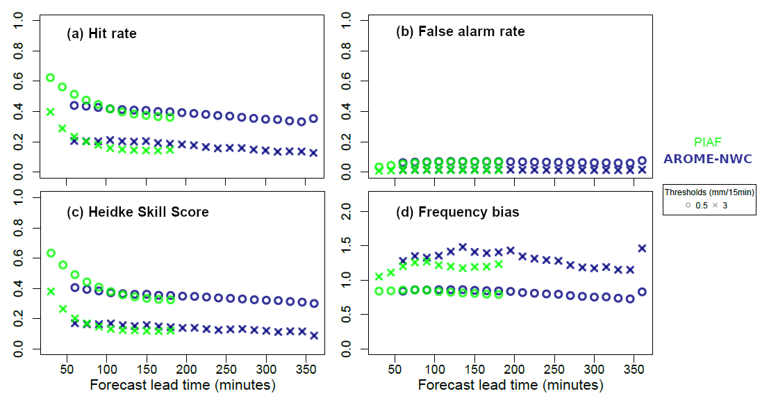
Figure 5(a) Hit rate, (b) false alarm rate, (c) Heidke skill score, and (d) frequency bias for thresholds: 0.5 mm/15 min and 3 mm/15 min computed for AROME-NWC (in blue) and PIAF (in green) over their respective forecast ranges for 15 min rain accumulation over the box displayed in Fig. 1.
The PIAF root mean square error increases with lead time up to 2 h and decreases very slightly beyond this (Fig. 4b). During the very early forecast period it increases very quickly. This can be explained by the quality of the extrapolation of radar data, which deteriorate quickly with the lead time. Indeed, the effects of advection errors accumulate and increase with successive time steps. The mean error for PIAF is also negative, indicating an underestimation of the precipitation amount on average (Fig. 4a). A quick loss of PIAF accuracy is observed in Fig. 5 (decrease in hit rate and HSS) in the first hour of lead time. It is still decreasing up to 1 h 40 min and becomes stable thereafter. As well as for AROME-NWC too many high rainfall accumulations (3 mm/15 min) are forecast by PIAF (Fig. 5d).
Comparison of the skills of the two nowcasting systems reveals that for lead times in the range T+2 h to T+3 h, AROME-NWC obtains on average better results than PIAF. For lead times in the range T+1 h to T+2 h, the performance of the two forecasting systems is often close. At lead times less than 90 or 75 min, depending on the intensity of the rainfall forecast, the performance of PIAF generally exceeds that of AROME-NWC.
The PIAF results from the linear combination of AROME-NWC prediction fields and radar extrapolation. The weights given to each predictor are adjusted according to their recent performance against observations as described in Sect. 2.2.2. In general an important weight is given to the extrapolation in the first time steps and for longer forecast times the numerical prediction gains more importance to the point that the rainfall field is entirely provided by AROME-NWC at the end of the PIAF forecast. Note for example that for the latest PIAF lead times, the root mean square errors converge to AROME-NWC errors beyond 2.5 h (Fig. 4b). However, the quality of PIAF and AROME-NWC may not be equivalent for the same forecast horizon. Indeed, PIAF forecasts are systematically based on the latest available AROME-NWC run and therefore the forecast lead time for the AROME-NWC run used in PIAF may be older than that indicated in the PIAF assessment. Since the AROME-NWC availability time is 35 min, for an AROME-NWC run initiated at round hour H, only PIAF forecasts initiated between H+40 min and H+95 min will use this run, and those between H and H+35 min will use the AROME-NWC run launched at H−1. Thus the same lead time of two PIAF forecasts does not necessarily rely on the same lead time of the two associated AROME-NWC runs. Differences between PIAF and AROME-NWC skills at the last PIAF forecast lead times may also be explained in several cases by the fact that PIAF does not switch completely to AROME-NWC (e.g. cases where AROME-NWC is too far away from observations over the last 6 h).
The main drawback of the point-to-point verification, especially in the case of convective situations, is to give significant weight to even small location errors (the so-called double penalty, Anthes, 1983; Gilleland et al., 2009). To give more credit to “close” forecasts a fuzzy method was used to measure the similarity between forecasts and observations in local neighbourhoods of the observations. Fraction skill scores (FSS, Roberts and Lean, 2008) were applied to compare forecast and observed coverage of rain exceeding certain thresholds in spatial windows of increasing size. The FSS were also used to compare AROME-NWC and PIAF and to analyse their performance with the forecast range. The five neighbourhood scales used are 1, 5, 10, 20 and 40 km, and 6,× 15 min precipitation thresholds of 0.5, 1, 2, 3, 5 and 10 mm were selected. Figures 6 and 7 show the 10-events mean FSS results for the various thresholds and window sizes at each forecast lead time for AROME-NWC and PIAF, respectively. As might be expected, the greatest skill (highest FSS values) is associated with the largest window and the smallest threshold while the lowest skill (FSS values near 0) is associated with the smaller spatial window and largest threshold. For AROME-NWC, at all lead times the FSS monotonically increases with the increase in spatial scale. For PIAF, there is a rapid and significant decrease in FSS values with the forecast range, up to 1 h 45 min lead time. It is mainly due to the decrease in the quality of the extrapolation forecast with time. The FSS computed from the PIAF precipitation forecast are generally better than those from AROME-NWC, at least for the first 90 min of forecast lead time.
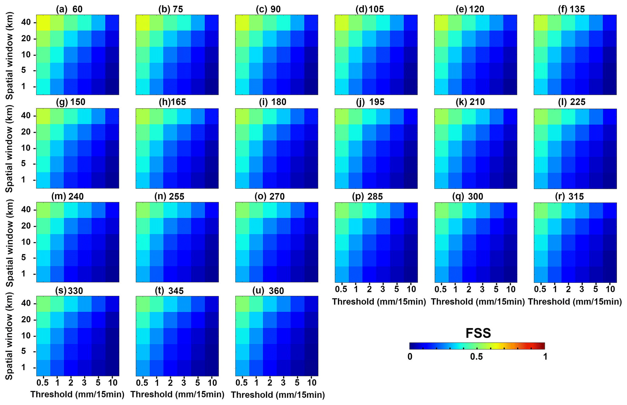
Figure 6The 10-events mean FSS obtained with AROME-NWC for the different precipitation thresholds (0.5, 1, 2, 3, 5 and 10 mm/15 min) and window sizes (1, 5, 10, 20 and 40 km) at each forecast lead time from (a) 60 min to (u) 360 min.
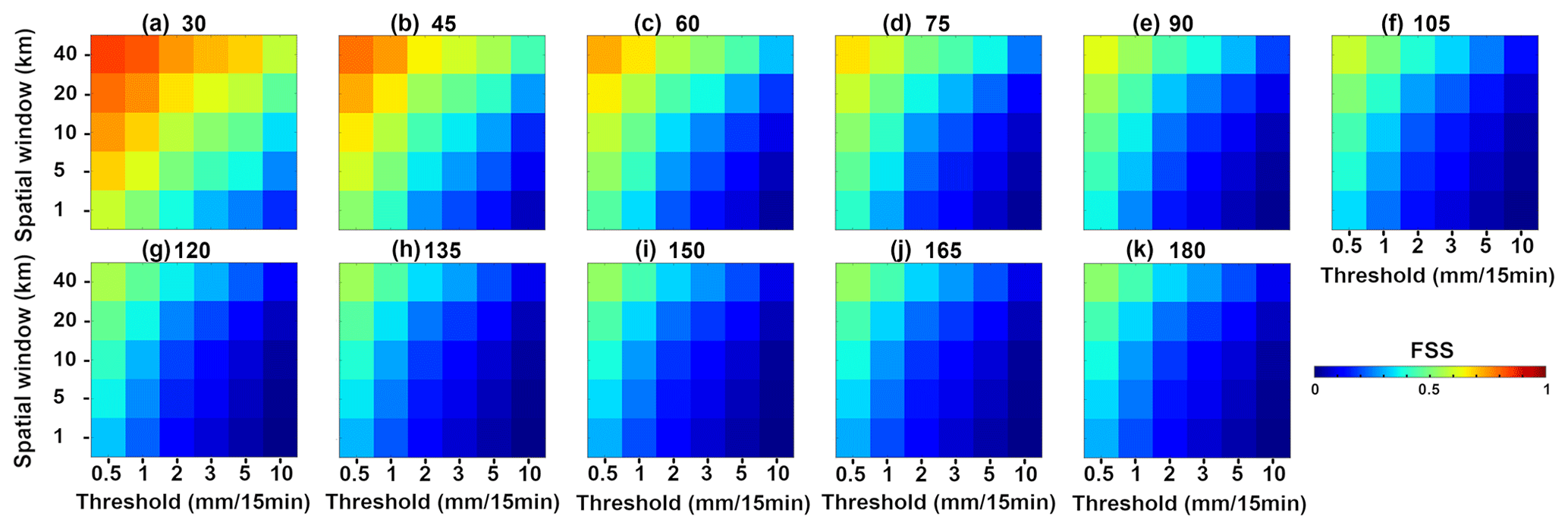
Figure 7The 10-events mean FSS obtained with PIAF for the different precipitation thresholds (0.5, 1, 2, 3, 5 and 10 mm/15 min) and window sizes (1, 5, 10, 20 and 40 km) at each forecast lead time from (a) 30 min to (k) 180 min.
In order to verify the forecast performance of AROME-NWC and PIAF, two verification methods were used: a traditional point-to-point verification and a neighbourhood spatial technique using FSS. The results obtained with these two methods are similar and can be summarized as follows: a quick loss of PIAF accuracy is observed on the very first lead times, its performance is higher than AROME-NWC up to 1 h 15 min/1 h 30 min of forecast but not necessarily beyond.
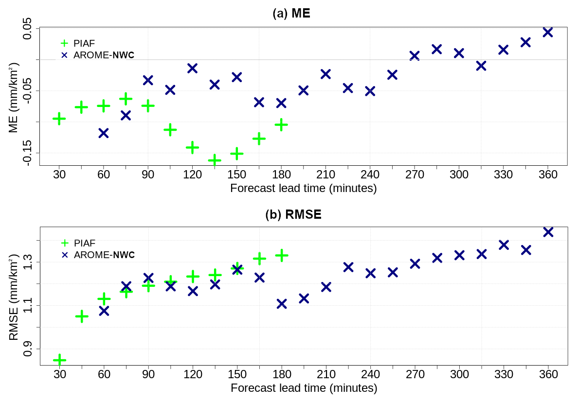
Figure 8(a) Mean and (b) root mean square errors for AROME-NWC (in blue) and PIAF (in green) over their respective forecast ranges for 15 min rain accumulation forecasts averaged over the catchments.
3.2 Evaluation of the rainfall nowcasting at the catchment scale
To complete and verify the conclusions of the point-to-point evaluation, the rainfall forecasts averaged over the catchments were also studied. Indeed, the amount and the location of rainfall forecasts at the catchment scale are essential for hydrological response forecast (Yates et al., 2006; Anquetin et al., 2005). The studied watersheds are those specified in Table 2.
Just as before, the mean and root mean square errors over watersheds are shown as a function of lead time in Fig. 8 for 15 min cumulated rainfall. The root mean square errors for AROME-NWC increase with the lead time. This increase is not strictly monotonous and is noisy due to the size of the sample: for example, a slight improvement in scores for AROME-NWC can be seen for lead times between 165 and 210 min (Fig. 8b). At lead times up to 4 h and 15 min, AROME-NWC underestimates on average the rainfall accumulations (Fig. 8a). The largest overestimates are observed for the events of 2015 and mid-October 2018, as shown by the interquartile ranges in Fig. 9, which represent the forecast error distributions (forecast values - observed values) of AROME-NWC and PIAF. The hit rate, the false alarm and the HSS vary little with the forecast lead time for the lowest threshold (0.5 mm/15 min) whereas the signal is more noisy for the 3 mm/15 min threshold with the hit rate and the HSS deteriorated with the lead time (blue markers for AROME-NWC in Fig. 10). For the higher rainfall intensities, the frequency bias increases with the lead time and is significantly greater than 1, indicating that AROME-NWC overpredicts these rainfall intensities. There is a loss of PIAF forecast accuracy with increasing forecast lead time (Fig. 8b). As seen previously for the point-to-point evaluation, the root mean square errors increase very rapidly over the first hour of the forecast.
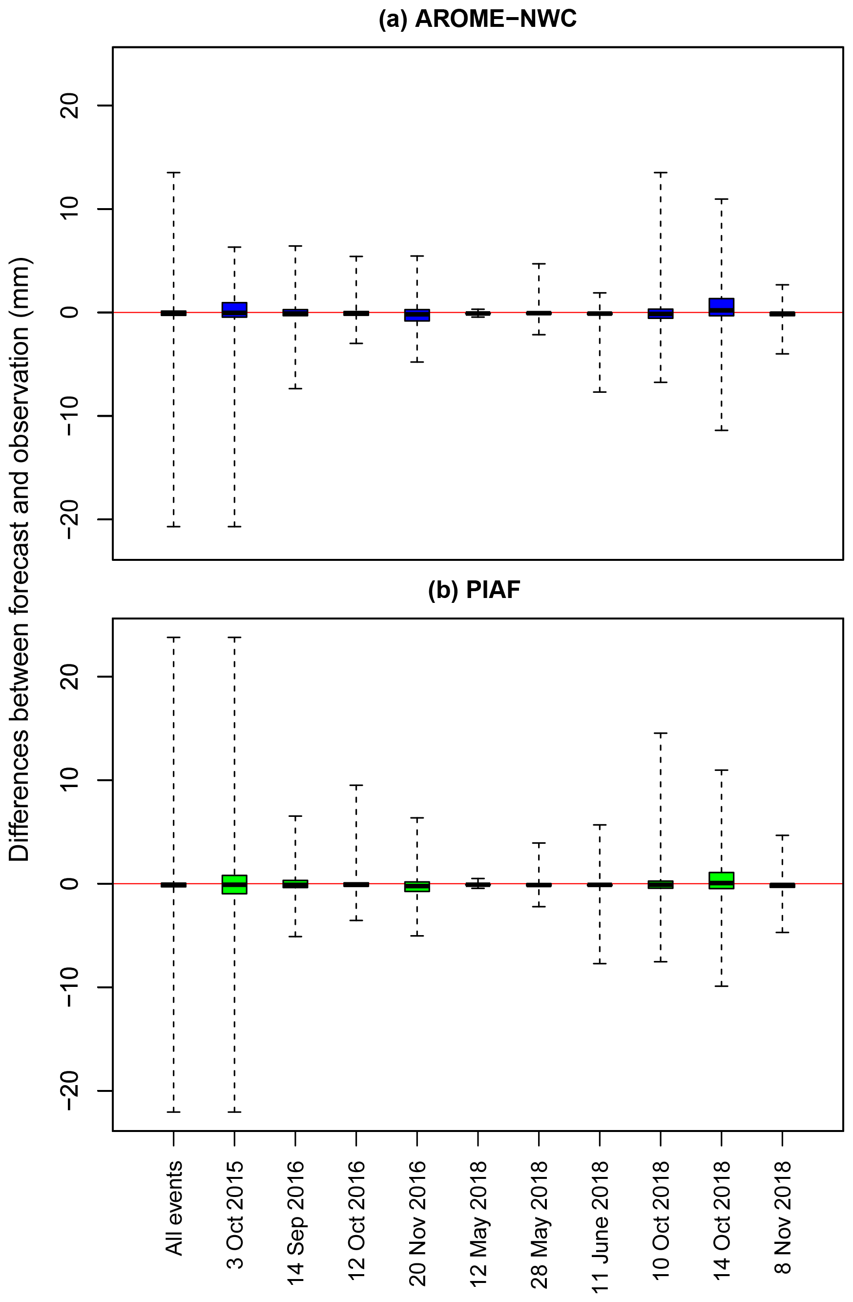
Figure 9Distributions of average rainfall forecast errors over catchment areas (forecast values – observed values) for (a) AROME-PI (lead times in the range T+45 min to T+6 h), and (b) PIAF (lead times in the range T+15 min to T+3 h) for all events and by event. The lower edge of the boxplots corresponds to the first quartile, the central line to the median and the upper edge to the third quartile of the values taken by these errors (the whiskers go up to the extreme values).
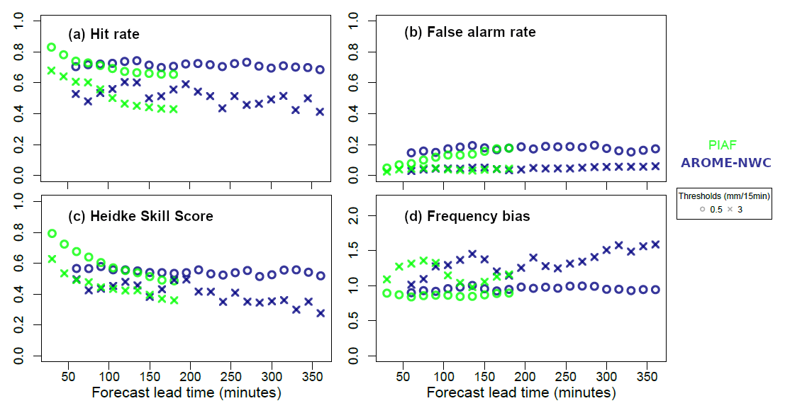
Figure 10(a) Hit rate, (b) false alarm rate, (c) Heidke skill score, and (d) frequency bias for thresholds: 0.5 mm/15 min and 3 mm/15 min computed for AROME-NWC (in blue) and PIAF (in green) over their respective forecast ranges for 15 min rain accumulation forecasts averaged over the catchments.
On average, PIAF rain accumulation forecasts are lower than those observed. The most significant forecast errors are due to the event of 3 October 2015 and more particularly on the Brague river at Biot where the extremes of error in 15 min rainfall forecasts are approximately ±20 mm. In terms of categorical scores (green markers for PIAF in Fig. 10), there is a visible decrease in the hit rate and HSS as a function of the forecast lead time for the two rainfall thresholds studied. The frequency bias is close to 1 for the 0.5 mm/15 min threshold and greater than 1 for the higher threshold.
Finally, the results of both verification methods (point-to-point and catchment scale comparisons of observed and forecast rainfall) generally lead to the same conclusions. The performance of PIAF is very good to good over the first hour of forecasting, but it deteriorates very quickly, to reach about the same or even a lower skill than AROME-NWC beyond about 1 h 15 min/1 h 30 min of forecasting. Between 2 and 3 h of forecasting, AROME-NWC performs better or at the same level as PIAF. It is worth mentioning that the values of the scores as a function of lead time show more variability from one lead time to the next compared to those of the point-to-point evaluation. This might be due to a smaller size of the evaluation sample.
3.3 Hydrological evaluation for two case studies
The potential of AROME-NWC and PIAF for flash flood nowcasting is introduced through the running of hydrological simulations using ISBA-TOP for two French major events occurred that on 3 October 2015 and on 14–15 October 2018 (see for example Fig. 11). These two remarkable events, which are part of the sample used for the rainfall assessment were selected for their significant hydrometeorological characteristics with very intense precipitation and river overflows. The evaluation aims at addressing the following question: how many hours of anticipation on floods can we have at most in terms of intensity and temporality of the flood peaks using rainfall nowcasting? From all the hydrological forecasts provided by ISBA-TOP driven by the rainfall forecast of October 2015 and 2018 (Table 2), the best anticipation of three phenomena was studied per watershed. These are
-
the start of increased discharge, defined here as an increase of at least 5 m3 s−1 in 1 h;
-
the right order of magnitude of the peak flow value (meaning an error of less than 30 % with respect to the reference peak discharge);
-
the peak time which is also the start of the recession limb.
For a given discharge forecast, the anticipation of one of these phenomena is calculated as the duration between two moments in time: the starting time of the rainfall forecast and the time of the phenomenon in the reference hydrograph (rainfall estimates as input to ISBA-TOP). The results are presented in Tables 4 and 5. The objective of these tables is to represent the behaviour of the best discharge forecasts for each watershed. They also provide a concise and comprehensive view of the results. For the peak time phenomenon, the anticipation period is only considered if the forecast and reference phenomenon occur at the same time. For the phenomena start of increased discharge and flood peak of the right intensity, a 1 h delay between forecast and reference is accepted. A different colour is assigned depending on the error between the reference flood peak and the forecast flood peak. If the difference between forecast and reference intensity is less than 10 %, it is coloured green, if the error is between 10 % and 20 %, it is coloured orange and if it is between 20 % and 30 %, it is coloured red.
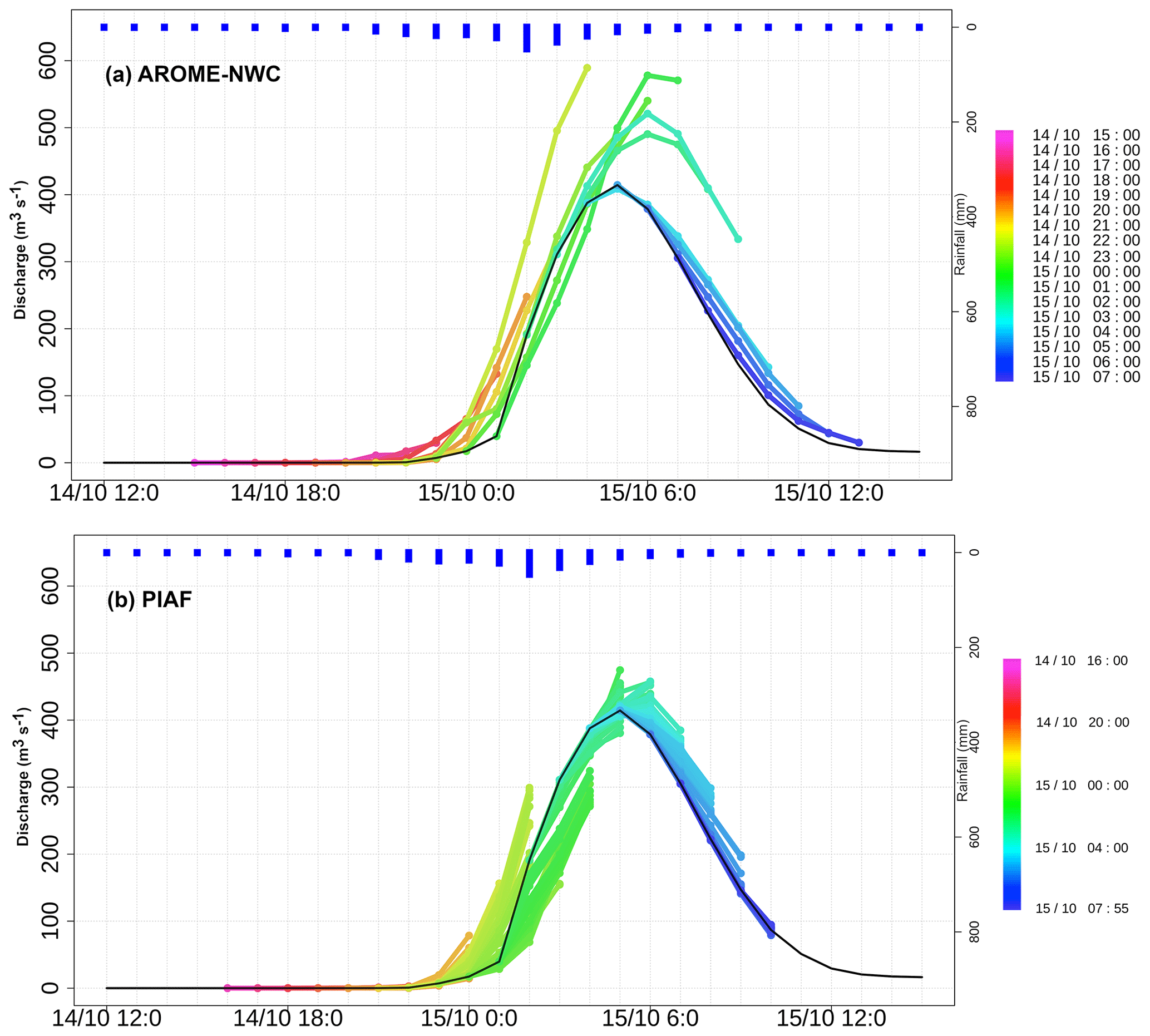
Figure 11Discharge time series simulated by ISBA-TOP driven by ANTILOPE (black curve), by (a) AROME-NWC and by (b) PIAF for the case 15 October 2018 for the Orbiel river at Bouilhonnac (watershed No. 4). The reverse histogram represents the ANTILOPE hourly rainfall averaged over the catchment.
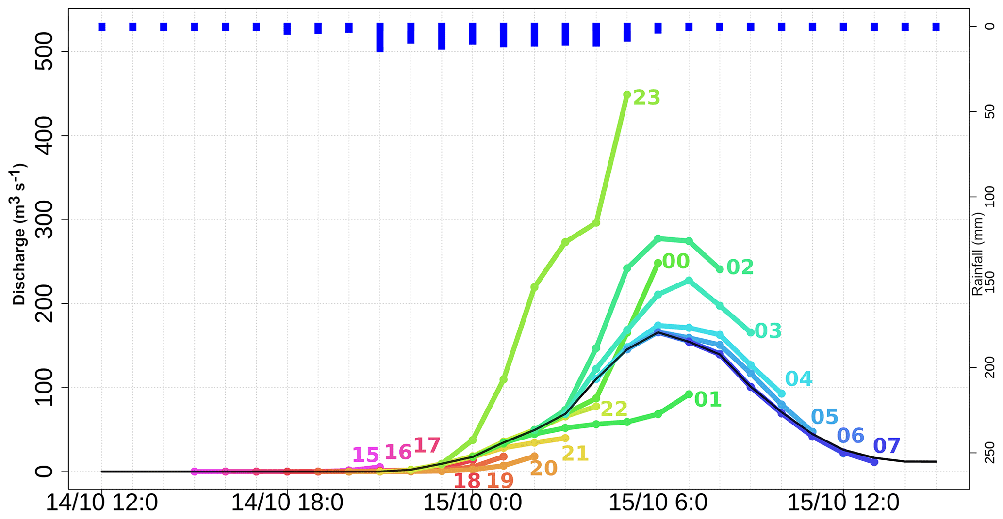
Figure 12Discharge time series simulated by ISBA-TOP driven by ANTILOPE rainfall estimates (black curve) and by AROME-NWC forecasts (coloured curves with forecasts starting from 14 October 15:00 UTC to 15 October 07:00 UTC) for the Fresquel river at Pezens (watershed No. 1). The reverse histogram represents the ANTILOPE hourly rainfall averaged over the catchment.
Table 3Best anticipation of the rise in flow, peak value and peak timing simulated with ISBA-TOP driven by the AROME-NWC rainfall forecast for the Fresquel river at Pezens on 14–15 October 2018. For more explanation on how to read the table, see Sect. 3.3.

Table 4Best anticipation of the rise in flow, peak value and peak timing simulated with ISBA-TOP driven by the AROME-NWC rainfall forecast for the watersheds affected during the events of October 2015 and 2018. The green colour (respectively orange, red) indicates an intensity error on the forecast peak lower than 10 % (respectively 20 %, 30 %) compared to the reference peak. Streamflow observations which were provided by the French HYDRO data bank (http://www.hydro.eaufrance.fr/, last access: 11 March 2020) or by HyMeX post-event surveys are for information purposes only. For more explanation on how to read the table, see Sect. 3.3.
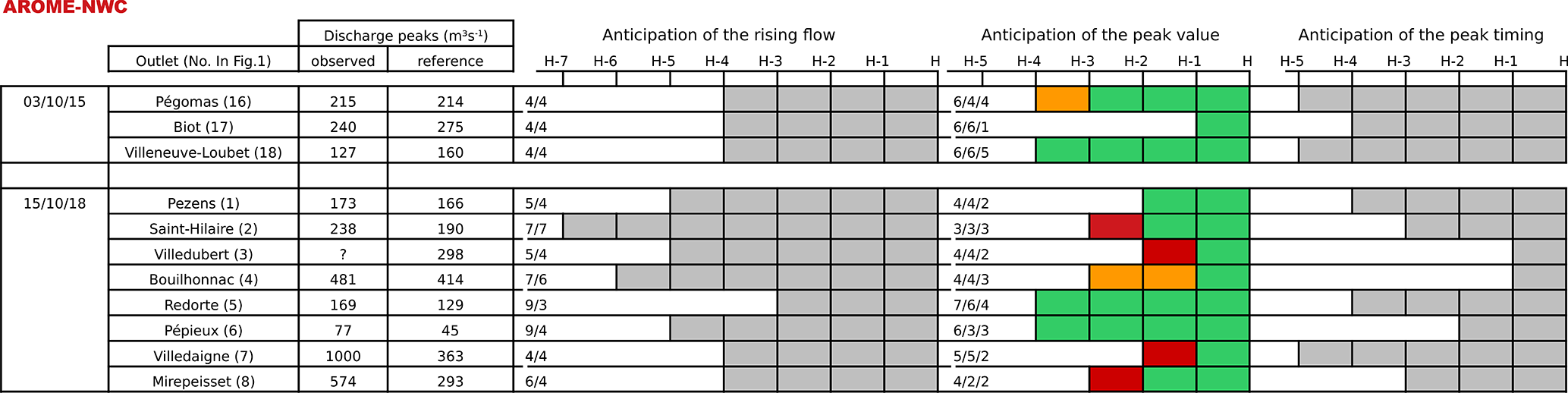
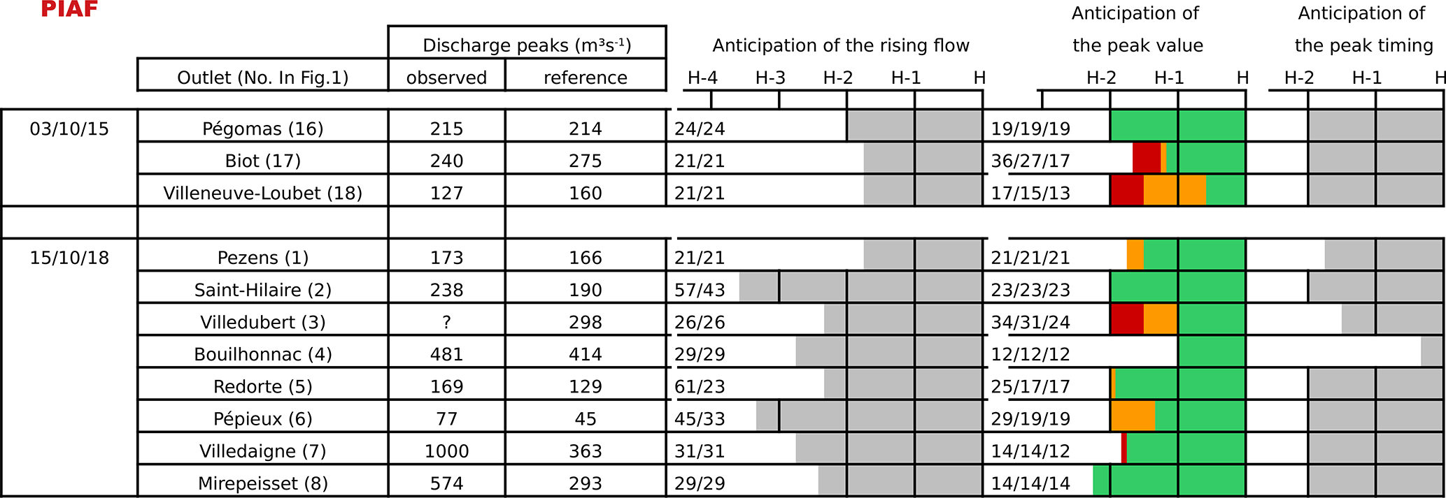
Table 5Best anticipation of the rise in flow, peak value and peak timing simulated with ISBA-TOP driven by the PIAF rainfall forecast for the watersheds affected during the events of October 2015 and 2018. The green colour (respectively orange, red) indicates an intensity error on the forecast peak lower than 10 % (respectively 20 %, 30 %) compared to the reference peak. Streamflow observations which were provided by the French HYDRO data bank (http://www.hydro.eaufrance.fr/, last access: 11 March 2020) or by HyMeX post-event surveys are for information purposes only. For more explanation on how to read the table, see Sect. 3.3.
To facilitate the reader's understanding of the tables, the line summarizing simulations for the Fresquel river at Pezens obtained by ISBA-TOP driven by AROME-NWC forecasts (Table 3, coming from Table 4) is taken as an example and is now detailed. Associated discharge time series are shown in Fig. 12.
-
In the reference simulation (in black in Fig. 12), the flow starts increasing at 23:00 coordinated universal time (UTC) on 14 October. To calculate the anticipation on this rise, we look for the oldest run which forecasts a rise at 22:00, 23:00 or 00:00 UTC. In this case, it is the run starting at 18:00 UTC, so the anticipation on the rise is 5 h. In the column “anticipation of the rising flow” of Table 3, we grey out 5 h before the hour of the phenomenon. To have an idea of the number of cases for which the flow rises are not forecast at the right time, we indicate in the same column of the table the number of runs launched before the flood start time on the reference hydrograph (before 23:00 UTC here) which forecast a rise, and among them the number which forecast a rise at ±1 h before the reference time. Here, five runs starting before 23:00 UTC forecast a rise (those from 18:00 to 22:00 UTC), four of them between 22:00 and 00:00 UTC (all except the run starting at 20:00 UTC which forecasts a rise 2 h later). In the column “anticipation of the rising flow” of Table 3, “” is thus written.
-
The reference peak, with an intensity of 166 m3 s−1, is simulated at 06:00 UTC on 15 October. Flood peaks are simulated by ISBA-TOP driven by the AROME-NWC forecasts starting from 02:00 to 05:00 UTC. To evaluate the anticipation on peak intensity, all peaks forecast at 06:00 UTC on 15 October ±1 h are considered. Among the runs mentioned, only those starting at 04:00 and 05:00 UTC simulate a flood peak with an intensity error of less than 30 %. The earliest run (starting at 04:00 UTC) is represented in the table: the anticipation on the right intensity of the flood peak is thus 2 h. For this forecast starting at 04:00 UTC, the difference between the forecast peak and the reference peak is less than 10 %, so the 2 h before the hour H are coloured green in the column “Anticipation of the peak value” in Table 3. To have an idea of the number of cases where a flood peak is forecast with an intensity close (or not) to the reference one, a triplet of values separated by slashes is indicated in the same column. These values correspond in the following order: to the total number of forecasts which forecast a flood peak, to the number of forecasts which forecast a flood peak at ±1 h of the reference peak and to the number of forecasts which forecast a flood peak at ±1 h of the reference peak and whose intensity error is less than 30 %. In this case for the event of 15 October 2018, among the 17 AROME-NWC forecasts used, 4 simulate a flood peak (runs starting between 02:00 and 05:00 UTC), 4 present a peak timing error of at most 1 h, but only 2 with an intensity error of less than 30 % (forecasts starting at 04:00 and 05:00 UTC). In the column “Anticipation of the peak value” of Table 3, “” is written.
-
The peak in the reference hydrograph occurs at 06:00 UTC. The first forecast that triggers a recession at the right time is that of 02:00 UTC, the anticipation on the peak time is therefore 4 h. So 4 h are greyed in the column “Anticipation of the peak timing” of Table 3. Note that the flood peak simulated with this run starting at 02:00 UTC is very overestimated. The anticipation of the right intensity of the flood peak does not always coincide with the anticipation of the time of the flood peak. If, as in this example, the duration of the anticipation of the right intensity of the flood peak is shorter than that of the peak timing, it means that older runs anticipate flood peaks but with a strong overestimation or underestimation. On the contrary, a duration of anticipation of the good intensity of the flood peak greater than that of the peak timing indicates that the predicted intensity of the flood peak was right at ±1 h but that the exact time of the flood peak was predicted only later. Note that to take into account the actual availability time of the rainfall forecasts, this time should be subtracted from the anticipation time indicated in the tables.
Among the best hydrological scenarios simulated with the AROME-NWC rainfall forecasts, the start of rising flow is anticipated at least 2 h ahead, regardless of the event (Table 4). In most cases, the anticipation is more than 4 h, and even, for the Orbiel and Lauquet rivers, an increase in flows is forecast up to 6 or 7 h in advance at the reference peak time ±1 h. Anticipation time is not proportional to the size of the watersheds, i.e. the smaller catchments with the lowest concentration times do not necessarily have a shorter anticipation time. Among the runs forecasting a rise of discharge, there are errors in peak timing greater than 1 h (for the 14 October 2018 case in particular, see in the column '“Anticipation of the rising flow” in Table 4), the time of the first rise of discharge is most often simulated too early. This is the case of the Ognon river at Pépieux where the start of the rising limb is anticipated 14 h in advance. Although hydrological information can be extracted from these simulations, considering them as true flood signals could yield hits but could also entail false alarms. Among the hydrological simulations based on PIAF rainfall forecasts, the best anticipation times of the onset of increasing discharge are always greater than 1 h and 15 min and reach 3 h and 45 min on the Lauquet river at Saint-Hilaire (Table 5).
The coloured cells in the column “Anticipation of the peak value” in Tables 4 and 5 indicate the best anticipation time of flood peak intensities. For the simulations based on AROME-NWC, the maximum anticipation on the flood peak with an error of the intensity lower than 10 % (green cells Table 4), ranges from 1 to 4 h depending on the catchment. Considering the forecast peaks for which the error of the peak intensity is higher (error between 10 % and 30 %) allows a gain of up to 1 or 2 h, as in the case of the Orbiel basin. With a tolerance of 20 % error of the intensity of the flood peak, the anticipation ranges from 1 to 4 h. In the simulations based on PIAF forecasts, the anticipation of the correct intensity of the flood peak (error less than 10 %, green cells in Table 5) is between 35 min and 2 h and 15 min. Considering the anticipation on the more erroneous intensity peaks allows an additional anticipation of 1 h and 25 min for the Loup river at Villeneuve-Loubet. For the simulated peaks with an intensity error of less than 30 %, the possible anticipation of flood peaks with ISBA-TOP can be estimated at approximately 1 h 30 min/2 h, which is an order of magnitude consistent with that found for a satisfactory performance of the nowcasting system during the rainfall forecasts evaluation.
For all the catchments, the peak times based on the AROME-NWC rainfall forecasts are anticipated with a maximum of 1–5 h (column “Anticipation of the peak timing” of Table 4). Flood recession in the catchments affected by the 3 October 2015 case is systematically anticipated 4 or 5 h in advance, this anticipation time is more variable for the 15 October 2018 event. In simulations based on PIAF rainfall forecasts, the start of the receding limb is in general forecast 1 h 30 min, 2 h ahead at best, except for the Orbiel river at Bouilhonnac, where the advance is only 20 min (Table 5).
These results obtained for two major flash flood events are therefore indicative of the promising use of AROME-NWC or PIAF rainfall forecasts for hydrological forecasting with an anticipation of peak intensity, timing, and first rise of discharge that can reach several hours.
The Mediterranean regions are regularly exposed to heavy rainfall events, which can trigger devastating flash floods. In these situations, hydrometeorological forecasts up to a few hours are crucial for increasing the preparedness of the authorities and planning the intervention of emergency services. In the current study, the potential of two nowcasting systems recently developed at Météo-France, has been assessed for forecasting Mediterranean intense rainfall events and floods. Precipitation forecasts were evaluated in southeastern France for 10 past heavy precipitation events using a point-to-point approach and an areal verification over watersheds affected by floods. The availability time of the rainfall forecast, which is of non-negligible time at the nowcasting ranges (few minutes to 6 h) was taken into account to consider constraints of forecasters during real-time operations. These assessments for a large area in the south east and for the catchments affected by the floods lead to the conclusion that:
-
PIAF is of very good quality over the first hour of forecasting, thanks in particular to the quality of the radar extrapolation. AROME-NWC is of good quality throughout its forecast, even if its skills tend to decrease slightly with the lead time.
-
Heavy rain is predicted too often with AROME-NWC and PIAF.
-
PIAF is of higher quality than AROME-NWC on the very first lead times. This quality deteriorates very quickly, to reach a quality comparable (or even lower) than AROME-NWC beyond about 1 h 15 min/1 h 30 min of forecast. For lead times between 2 and 3 h, the performance of AROME-NWC is higher or equivalent to that of PIAF in general.
This evaluation points out the strengths and weaknesses of the nowcasting system types during extreme events that should be considered before selecting the best method or combination for future studies or operational purposes. Depending on the accuracy of the initial radar rainfall estimation and the spatial distribution and intensity of the precipitation, radar extrapolation can provide valuable nowcasting information in the very short-term forecast. However due to dynamical evolution of precipitation, especially in convective situations, there is a rapid decrease in accuracy with forecasting lead time. The above results show that blending the extrapolation of radar data with numerical prediction forecasts allows improvement of the nowcasting accuracy and to extend the lead time beyond the characteristic 1 h lead time of extrapolation methods. Indeed, the use of numerical forecast helps to overcome the limitations of extrapolation at the initiation and decaying stages of convective cells and to take the impact of the relief on the evolution of precipitation better into account. The use of numerical forecasts is particularly appropriate for lead times greater than 2 h if the numerical prediction system has been designed for nowcasting purposes. Resulting forecasts are thus frequently refreshed with new observations and are produced with a higher time resolution and a reduced calculation time compared to the time needed to run other numerical systems.
This study also highlights the benefit of the combined use of rainfall nowcasting and a distributed hydrologic model for flash flood forecasting. It was investigated for two catastrophic French events that occurred on 3 October 2015 and on 14–15 October 2018. The hydrological forecasts for small watersheds are sensitive to both the rainfall intensity and location. Nowcasting provides relevant information up to a range of a few hours in terms of amount, timing, and basin-specific locations of rainfall. Of the three phenomena studied (start of increased discharge, peak time and value), the best anticipation times for AROME-NWC and PIAF are found in the increase in discharge in general. The peak time and intensity can be anticipated up to 1–5 h in advance from the AROME-NWC forecasts. Up to 1 h and 30 min, or 2 h, PIAF allows peak value and time to be well forecasted. Even if this hydrological assessment of the nowcasting systems provides positive and encouraging results for flash flood forecasting, simulations could certainly be improved by using the propagation capability of the hydrological model. By letting the hydrological model route the water a few hours after the end of the rainfall forecast, anticipation times could be increased. This point could be addressed within the framework of the French PICS project (Payrastre et al., 2019) as well as the use of other hydrological models and new case studies for further analysis.
The mean error (ME) measures the averaged error magnitude as follows:
where oi and fi are the observed and forecast values, respectively and N the number of forecast-observation pairs.
It ranges from −∞ to +∞ and is zero if the forecast is perfect. A positive value indicates overestimation, a negative value indicates underestimation. Note with this score, strong errors in the opposite direction can compensate each other.
The root mean square error (RMSE) is defined as follows:
It ranges from 0 to +∞ and is zero if the forecast is perfect.
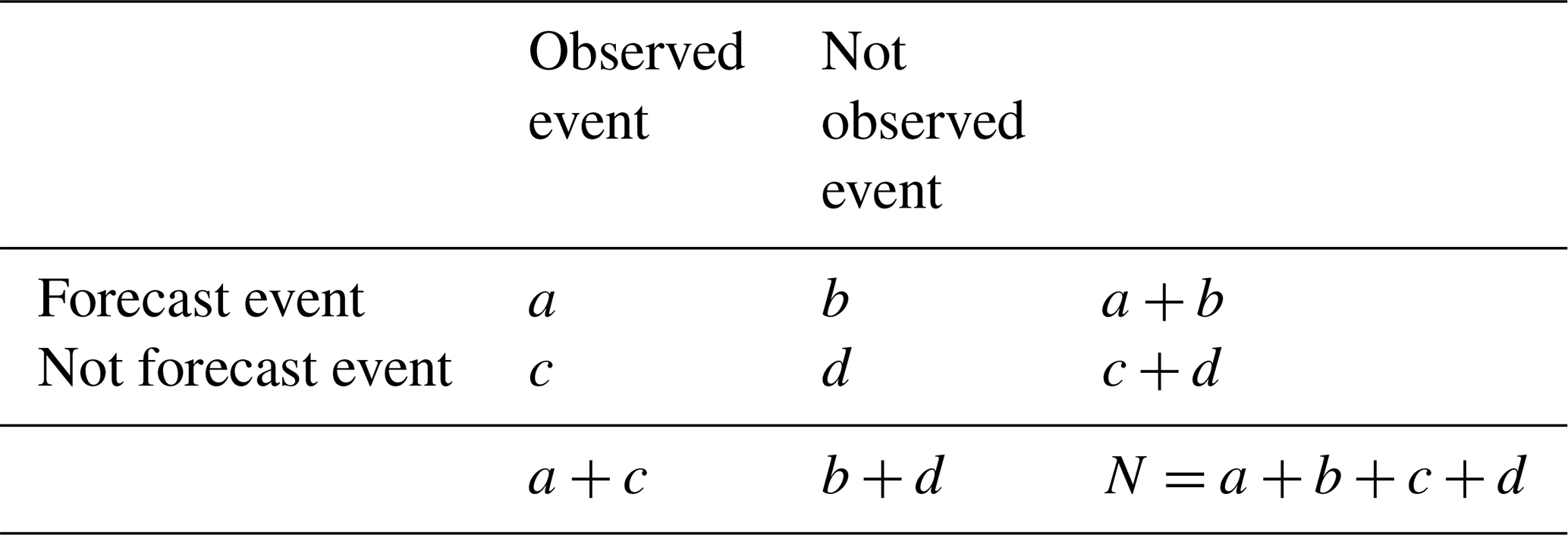
For binary events a categorical contingency table can be built such as Table A1. It is often used to compute categorical verification scores.
Table A1Contingency table for a binary event. The table fully describes the joint distribution of forecast and observation for N forecast/observation pairs.
-
The hit rate or probability of detection is defined as follows:
It ranges from 0 to 1 (1 for a perfect forecast).
-
The false alarm rate or probability of false detection is defined as follows:
It ranges from 0 to 1 (0 for a perfect forecast).
-
The Heidke skill score (HSS) measures the fraction of correct forecasts after eliminating the correct random forecasts:
It ranges from −∞ to 1 (1 for a perfect forecast).
-
Frequency bias is defined as follows:
It ranges from 0 to ∞.
A1 Gerrity score
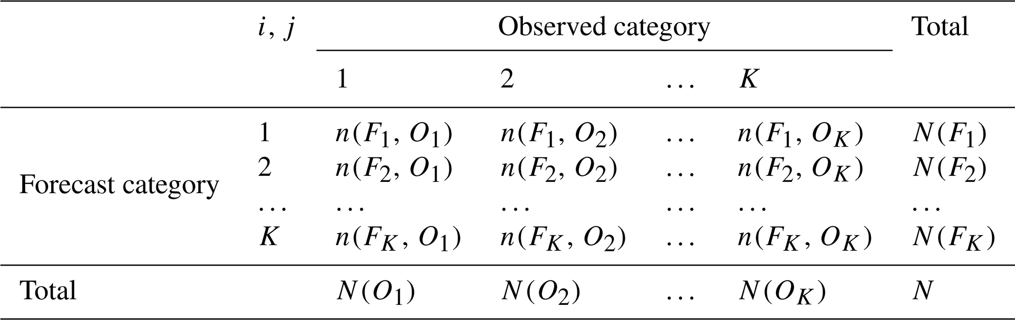
The Gerrity score (Gerrity, 1992) is based on a multicategory contingency table such as Table A2. In the PIAF algorithm, 6 rain thresholds: 0.05; 0.1; 0.2; 0.4; 0.8 and 1.6 mm/5 min are considered in the multicategory contingency table.
Table A2K-category contingency table. n(Fi, Oj) is the number of forecast/observed pairs for which the forecast is in category i and the observation in category j. N(Fi) indicates the total number of forecasts in the category i, N(Oj) indicates the total number of observations in the category j and N the total number of forecast/observed pairs.
The Gerrity score is defined as follows:
where sij are the elements of a matrix characterized by on the diagonal and elsewhere, with and the frequency of observations in category t.
It ranges from −1 to 1 (1 for a perfect forecast).
A2 FSS
The fractions skill score (FSS, Roberts and Lean, 2008) allows evaluation of the quality of a forecast for several intensity thresholds with a certain spatial tolerance. The idea is to compare the observed and forecast probabilities of an event in spatial windows of increasing size. The FSS is defined by
with N the number of points in the considered spatial window, pf,i the forecast fraction of grid points that exceed the threshold in this window and po,i the observed one.
In concrete terms, the observation and forecast fields are made binary by assigning the value 1 to pixels associated with exceeding the studied threshold and 0 in the opposite case. A neighbourhood size is set. Then, within the neighbourhood of each pixel in the area of study, the fraction of observed and forecast points above the intensity threshold is calculated.
The FSS ranges from 0 to 1, close to 1 for a good forecast and close to 0 in the opposite case. In general, as the spatial tolerance increases, the FSS increases, and as the intensity thresholds increases, the FSS decreases.
The Shuttle Radar Topographic Mission (SRTM) 90 m digital elevation data, originally produced by NASA, are available at the Consortium for Spatial Information of the Consultative Group for International Agricultural Research (CGIAR-CSI) geoportal (https://cgiarcsi.community/data/srtm-90m-digital-elevation-database-v4-1; CGIAR CSI, 2022).
AL performed the computational work. BV and VD supervised this work. All co-authors collaborated, interpreted the results, wrote the paper and replied to the comments from the reviewers.
The contact author has declared that neither they nor their co-authors have any competing interests.
Publisher's note: Copernicus Publications remains neutral with regard to jurisdictional claims in published maps and institutional affiliations.
This article is part of the special issue “Hydrological cycle in the Mediterranean (ACP/AMT/GMD/HESS/NHESS/OS inter-journal SI)”. It is not associated with a conference.
The authors would like to express their gratitude for access to useful data and discussions with the members of the nowcasting team at Météo-France, and especially Céline Jauffret, Philippe Cau and Nicolas Merlet.
This research was performed within the framework of the HyMeX programme (MISTRALS grants) and is a contribution to the French project PICS (ANR-17-CE03-0011).
This paper was edited by Giuseppe Tito Aronica and reviewed by two anonymous referees.
Alfieri, L., Thielen, J., and Pappenberger, F.: Ensemble hydro-meteorological simulation for flash flood early detection in southern Switzerland, J. Hydrol., 424, 143–153, 2012. a
Anquetin, S., Yates, E., Ducrocq, V., Samouillan, S., Chancibault, K., Davolio, S., Accadia, C., Casaioli, M., Mariani, S., Ficca, G., Gozzini, B., Pasi, F., Pasqui, M., Garcia, A., Martorell, M., Romero, R., and Chessa, P.: The 8 and 9 September 2002 flash flood event in France: a model intercomparison, Nat. Hazards Earth Syst. Sci., 5, 741–754, https://doi.org/10.5194/nhess-5-741-2005, 2005. a
Anthes, R. A.: Regional models of the atmosphere in middle latitudes, Mon. Weather Rev., 111, 1306–1335, 1983. a
Artinyan, E., Vincendon, B., Kroumova, K., Nedkov, N., Tsarev, P., Balabanova, S., and Koshinchanov, G.: Flood forecasting and alert system for Arda River basin, J. Hydrol., 541, 457–470, 2016. a
Auger, L., Dupont, O., Hagelin, S., Brousseau, P., and Brovelli, P.: AROME–NWC: a new nowcasting tool based on an operational mesoscale forecasting system, Q. J. Roy. Meteorol. Soc., 141, 1603–1611, 2015. a, b, c
Ballabio, C., Panagos, P., and Monatanarella, L.: Mapping topsoil physical properties at European scale using the LUCAS database, Geoderma, 261, 110–123, 2016. a
Berenguer, M., Corral, C., Sánchez-Diezma, R., and Sempere-Torres, D.: Hydrological validation of a radar-based nowcasting technique, J. Hydrometeorol., 6, 532–549, 2005. a, b
Beven, K. and Kirkby, M. J.: A physically based, variable contributing area model of basin hydrology/Un modèle à base physique de zone d'appel variable de l'hydrologie du bassin versant, Hydrolog. Sci. J., 24, 43–69, 1979. a
Borga, M.: Accuracy of radar rainfall estimates for streamflow simulation, J. Hydrol., 267, 26–39, 2002. a
Bouilloud, L., Chancibault, K., Vincendon, B., Ducrocq, V., Habets, F., Saulnier, G.-M., Anquetin, S., Martin, E., and Noilhan, J.: Coupling the ISBA land surface model and the TOPMODEL hydrological model for Mediterranean flash-flood forecasting: description, calibration, and validation, J. Hydrometeorol., 11, 315–333, 2010. a, b, c
Brousseau, P., Seity, Y., Ricard, D., and Léger, J.: Improvement of the forecast of convective activity from the AROME-France system, Q. J. Roy. Meteorol. Soc., 142, 2231–2243, 2016. a
Caumont, O., Bouttier, F., Brossier, C. L., Lovat, A., Mandement, M., Nuissier, O., Laurantin, O., and Eeckman, J.: The Catastrophic Case of Heavy Rainfall and Flash Flooding of 14–15 October 2018 in South-Western France: a Multi-Scale Observational and Modeling Analysis, in: 100th American Meteorological Society Annual Meeting, AMS, 10th European Conference on Severe Storms, 4–8 November 2019, Kraków, Poland, https://meetingorganizer.copernicus.org/ECSS2019/ECSS2019-158-1.pdf (last access: 20 May 2022), 2020. a
Cesa-Bianchi, N. and Lugosi, G.: Prediction, learning, and games, Cambridge University Press, https://ii.uni.wroc.pl/~lukstafi/pmwiki/uploads/AGT/Prediction_Learning_and_Games.pdf (last access: 20 May 2022), 2006. a, b
CGIAR CSI: SRTM 90 m Digital Elevation Database v4.1, CGIAR CSI [data set], https://cgiarcsi.community/data/srtm-90m-digital-elevation-database-v4-1, last access: 20 May 2022. a
Dixon, M. and Wiener, G.: TITAN: Thunderstorm identification, tracking, analysis, and nowcasting – A radar-based methodology, J. Atmos. Ocean. Tech., 10, 785–797, 1993. a
Dolcine, L., Andrieu, H., Sempere-Torres, D., and Creutin, D.: Flash flood forecasting with coupled precipitation model in mountainous Mediterranean basin, J. Hydrol. Eng., 6, 1–10, 2001. a
Drobinski, P., Ducrocq, V., Alpert, P., Anagnostou, E., Béranger, K., Borga, M., Braud, I., Chanzy, A., Davolio, S., Delrieu, G., Estournel, C., N Filali Boubrahmi, N., Font, J., Grubišić, V., Gualdi, S., Homar, V., Ivančan-Picek, B., Kottmeier, C., Kotroni, V., Lagouvardos, K., Lionello, P., Llasat, M. C., Ludwig, W., Lutoff, C., Mariotti, A., Richard, E., Romero, R., Rotunno, R., Roussot, O., Ruin, I., Somot, S., Taupier-Letage, I., Tintore, J., Uijlenhoet, R., and Wernli, H.: HyMeX: A 10-year multidisciplinary program on the Mediterranean water cycle, B. Am. Meteorol., Soc., 95, 1063–1082, 2014. a
Faroux, S., Kaptué Tchuenté, A. T., Roujean, J.-L., Masson, V., Martin, E., and Le Moigne, P.: ECOCLIMAP-II/Europe: a twofold database of ecosystems and surface parameters at 1 km resolution based on satellite information for use in land surface, meteorological and climate models, Geosci. Model Dev., 6, 563–582, https://doi.org/10.5194/gmd-6-563-2013, 2013. a
Gaillard, P. and Goude, Y.: Forecasting electricity consumption by aggregating experts; how to design a good set of experts, in: Modeling and stochastic learning for forecasting in high dimensions, Springer, 95–115, ISBN 978-3-319-18732-7, 2015. a
Gaume, E., Borga, M., Llassat, M. C., Maouche, S., Lang, M., and Diakakis, M.: Mediterranean extreme floods and flash floods, https://hal.archives-ouvertes.fr/hal-01465740/document (last access: 20 May 2022), 2016. a
Germann, U. and Zawadzki, I.: Scale dependence of the predictability of precipitation from continental radar images. Part II: Probability forecasts, J. Appl. Meteorol., 43, 74–89, 2004. a
Gerrity Jr., J. P.: A note on Gandin and Murphy's equitable skill score, Mon. Weather Rev., 120, 2709–2712, 1992. a, b
Gilleland, E., Ahijevych, D., Brown, B. G., Casati, B., and Ebert, E. E.: Intercomparison of spatial forecast verification methods, Weather Forecast., 24, 1416–1430, 2009. a
Golding, B.: Nimrod: A system for generating automated very short range forecasts, Meteorol. Appl., 5, 1–16, 1998. a, b
Habets, F., Noilhan, J., Golaz, C., Goutorbe, J., Laccarrère, P., Leblois, E., Ledoux, E., Martin, E., Ottlé, O., and Vidal-madjar, D.: The ISBA surface scheme in a macroscale hydrological model applied to the HAPEX-MOBILHY area. Part I: Model and database, J. Hydrol., 217, 75–96, 1999. a
Johnson, J., MacKeen, P. L., Witt, A., Mitchell, E. D. W., Stumpf, G. J., Eilts, M. D., and Thomas, K. W.: The storm cell identification and tracking algorithm: An enhanced WSR-88D algorithm, Weather Forecast., 13, 263–276, 1998. a
Kahle, D. and Wickham, H.: ggmap: Spatial Visualization with ggplot2, R J., 5, 144–161, 2013. a
Laroche, S. and Zawadzki, I.: Retrievals of horizontal winds from single-Doppler clear-air data by methods of cross correlation and variational analysis, J. Atmos. Ocean. Tech., 12, 721–738, 1995. a
Laurantin, O.: ANTILOPE: Hourly rainfall analysis merging radar and rain gauge data, in: Proceedings of the International Symposium on Weather Radar and Hydrology, 10–12 March 2008, Grenoble, France, 2–8, 2008. a
Li, L., Schmid, W., and Joss, J.: Nowcasting of motion and growth of precipitation with radar over a complex orography, J. Appl. Meteorol., 34, 1286–1300, 1995. a
Ligda, M. G.: Horizontal Motion of Small Precipitation Areas as Observed by Radar, PhD Thesis, 1953. a
Lovat, A., Vincendon, B., and Ducrocq, V.: Assessing the impact of resolution and soil datasets on flash-flood modelling, Hydrol. Earth Syst. Sci., 23, 1801–1818, https://doi.org/10.5194/hess-23-1801-2019, 2019. a, b
Masson, V., Champeaux, J.-L., Chauvin, F., Meriguet, C., and Lacaze, R.: A global database of land surface parameters at 1-km resolution in meteorological and climate models, J. Climate, 16, 1261–1282, 2003. a
Moisselin, J.-M., Cau, P., Jauffret, C., Bouissières, I., and Tzanos, R.: Seamless approach for precipitations within the 0–3 hours forecast-interval, in: European Nowcasting Conference, April 2019, Madrid, Spain, https://repositorio.aemet.es/bitstream/20.500.11765/10588/3/SPDA2_Moisselin_3ENC2019.pdf (last access: 20 May 2022), 2019. a, b, c
Noilhan, J. and Planton, S.: A simple parameterization of land surface processes for meteorological models, Mon. Weather Rev., 117, 536–549, 1989. a
Nuissier, O., Marsigli, C., Vincendon, B., Hally, A., Bouttier, F., Montani, A., and Paccagnella, T.: Evaluation of two convection-permitting ensemble systems in the HyMeX Special Observation Period (SOP1) framework, Q. J. Roy. Meteorol. Soc., 142, 404–418, 2016. a
Payrastre, O., Lebouc, L., Ayral, P. A., Brunet, P., Delrieu, G., Douvinet, J., Dramais, G., Javelle, P., Johannet, A., Adamovic, M., Adnes, C., Cantet, P., Chapuis, M., Coutouis, A., Creutin, J.-D., Gonzalez-Sosa, E., Ruin, I., Saint-Martin, C., Shabou, S., and Whilhelm, B. The October 2015 flash-floods in south eastern France: first discharge estimations and comparison with other flash-floods documented in the framework of the Hymex project, in: EGU General Assembly Conference Abstracts, vol. 18, p. 13912, https://ui.adsabs.harvard.edu/abs/2016EGUGA..1813912P/abstract (last access: 20 May 2022), 2016. a
Payrastre, O., Bourgin, F., Caumont, O., Ducrocq, V., Gaume, E., Janet, B., Javelle, P., Lague, D., Moncoulon, D., Naulin, J.-P., Perrin, C., Ramos, M.-H., Ruin, I., and the PICS project contributors: Integrated nowcasting of flash floods and related socio-economic impacts: The French ANR PICS project (2018–2021), Geophys. Res. Abstr., 21, 1, 2019. a
Pellarin, T., Delrieu, G., Saulnier, G.-M., Andrieu, H., Vignal, B., and Creutin, J.-D.: Hydrologic visibility of weather radar systems operating in mountainous regions: Case study for the Ardeche catchment (France), J. Hydrometeorol., 3, 539–555, 2002. a
Pinty, J. and Jabouille, P.: A mixed-phase cloud parameterization for use in mesoscale non-hydrostatic model: simulations of a squall line and of orographic precipitations, in: Conf. on Cloud Physics, Amer. Meteor. Soc., Everett, WA, 217–220, 1998. a
Poletti, M. L., Silvestro, F., Davolio, S., Pignone, F., and Rebora, N.: Using nowcasting technique and data assimilation in a meteorological model to improve very short range hydrological forecasts, Hydrol. Earth Syst. Sci., 23, 3823–3841, https://doi.org/10.5194/hess-23-3823-2019, 2019. a, b
Ricard, D., Ducrocq, V., and Auger, L.: A climatology of the mesoscale environment associated with heavily precipitating events over a northwestern Mediterranean area, J. Appl. Meteorol. Clim., 51, 468–488, 2012. a
Rinehart, R. and Garvey, E.: Three-dimensional storm motion detection by conventional weather radar, https://www.nature.com/articles/273287a0.pdf?origin=ppub (last access: 20 May 2022), 1978. a
Roberts, N. M. and Lean, H. W.: Scale-selective verification of rainfall accumulations from high-resolution forecasts of convective events, Mon. Weather Rev., 136, 78–97, 2008. a, b
Seity, Y., Brousseau, P., Malardel, S., Hello, G., Bénard, P., Bouttier, F., Lac, C., and Masson, V.: The AROME-France convective-scale operational model, Mon. Weather Rev., 139, 976–991, 2011. a
Silvestro, F. and Rebora, N.: Operational verification of a framework for the probabilistic nowcasting of river discharge in small and medium size basins, Nat. Hazards Earth Syst. Sci., 12, 763–776, https://doi.org/10.5194/nhess-12-763-2012, 2012. a
Silvestro, F., Rebora, N., Cummings, G., and Ferraris, L.: Experiences of dealing with flash floods using an ensemble hydrological nowcasting chain: implications of communication, accessibility and distribution of the results, J. Flood Risk Manage., 10, 446–462, 2017. a, b
Vié, B.: Méthodes de prévision d’ensemble pour l'étude de la prévisibilité à l'échelle convective desépisodes de pluies intenses en Méditerranée, PhD thesis, Paris Est, https://pastel.archives-ouvertes.fr/pastel-00805613/document (last access: 20 May 2022), 2012. a
Vincendon, B., Édouard, S., Dewaele, H., Ducrocq, V., Lespinas, F., Delrieu, G., and Anquetin, S.: Modeling flash floods in southern France for road management purposes, J. Hydrol., 541, 190–205, 2016. a, b, c
Vivoni, E. R., Entekhabi, D., Bras, R. L., Ivanov, V. Y., Van Horne, M. P., Grassotti, C., and Hoffman, R. N.: Extending the predictability of hydrometeorological flood events using radar rainfall nowcasting, J. Hydrometeorol., 7, 660–677, 2006. a
Weygandt, S. S., Smirnova, T., Benjamin, S., Brundage, K., Sahm, S., Alexander, C., and Schwartz, B.: The High Resolution Rapid Refresh (HRRR): an hourly updated convection resolving model utilizing radar reflectivity assimilation from the RUC/RR, in: Amer. Meteor. Soc. A, vol. 15, Preprints, 23rd Conf. on Weather Analysis and Forecasting/19th Conf. on Numerical Weather Prediction, 1–5 June 2009, Omaha, NE, https://ams.confex.com/ams/23WAF19NWP/techprogram/paper_154317.htm (last access: 20 May 2022), 2009. a
Yates, E., Anquetin, S., Ducrocq, V., Creutin, J.-D., Ricard, D., and Chancibault, K.: Point and areal validation of forecast precipitation fields, Meteorol. Appl., 13, 1–20, 2006. a