the Creative Commons Attribution 4.0 License.
the Creative Commons Attribution 4.0 License.
 | 18 May 2022
Advances in the hydraulic interpretation of water wells using flowmeter logs
Jesús Díaz-Curiel
Bárbara Biosca
Lucía Arévalo-Lomas
María Jesús Miguel
Natalia Caparrini
This paper reports on the methodology developed for a new hydraulic interpretation of flowmeter logs, allowing a better characterization of continental hydrological basins. In the course of a flowmeter log, different flow stretches are established, mostly corresponding to permeable layers (aquifers), among which there are other stretches mainly corresponding to less permeable layers (aquitards). In such hydrological basins of sufficient thickness, these flow stretches may not have the same hydraulic head. This fact brings about the need for a new hydraulic interpretation that provides the actual distribution of horizontal permeability throughout the aquifer at depth. The modified hydraulic interpretation developed in this study focuses on the differences of the effective pressure gradient (considered the difference between the hydraulic head in the well and the hydraulic head of each stretch) experienced by the different flow stretches along the well, due to the existence of different hydraulic heads. The methodology has been developed starting from a water well located in a multilayered aquifer within the so-called Madrid basin (the north-western part of the continental basin of the Tagus River), located in the centre of the Iberian Peninsula. In this well, a step-drawdown pumping test was conducted, in which the pumping rate versus drawdown and the specific capacity versus drawdown showed discrepancies with Darcian behaviour and an exponent of the Jacob equation of less than 1. Flowmeter logs were then recorded for different discharge rates and pump depths; the resulting water input from deeper permeable layers did not appear to show the expected relation with respect to drawdown. With the proposed methodology the results comply with the expected linearity and the cited discrepancies are solved.
- Article
(8409 KB) - Full-text XML
- BibTeX
- EndNote


One of the most interesting hydrogeological aspects of well pumping tests is that their results not only allow us to estimate the permeability and transmissivity obtained in the well, but that they can also be used to infer the behaviour of the aquifer when the lithological distribution of the basin in its location is known. This estimate of basin behaviour will be less accurate when knowledge of the lithology is local. In the case of step-drawdown pumping tests, this inference is generally known when the characteristic curves of the test show a conventional evolution, i.e. when the drawdown versus the extraction rate curve shows an increasing slope and the specific capacity decreases with drawdown. This is the case when, inside the well, in the near-wellbore zone or in the aquifer, head losses occur, whether linear or polynomial, whose effects are well recognized in step-drawdown pumping test curves (Helweg, 1994; Kawecki, 1995; Mathias and Todman, 2010).
These models provide an accurate representation of the aquifer behaviour for any pumping time. Among other results, Mathias and Todman (2010) found that the best fit was achieved by using a non-linear coefficient, called the “well loss coefficient”, which can be different for each step. The values of this coefficient were obtained using an analytical formula derived to relate this coefficient to the Forchheimer parameter. When the drawdown versus the extraction rate curve presents an increasing slope, as in the case of the step-drawdown test from Clark (1977) (a similar behaviour can be seen in the generic curves 2 and 3 shown in Fig. 1), there are different hydrogeological explanations. However, the slope decreases and the specific capacity versus the drawdown increases, i.e. when the hydric behaviour improves with increasing flow rate, as in the last two stages of the step-drawdown test from Van Tonder et al. (2001) (a similar behaviour can be seen in the generic curve 4 shown in Fig. 1). The only explanation known to date is that the well is not properly developed. In the following text, when such results occur, they are referred to as anomalous cases.
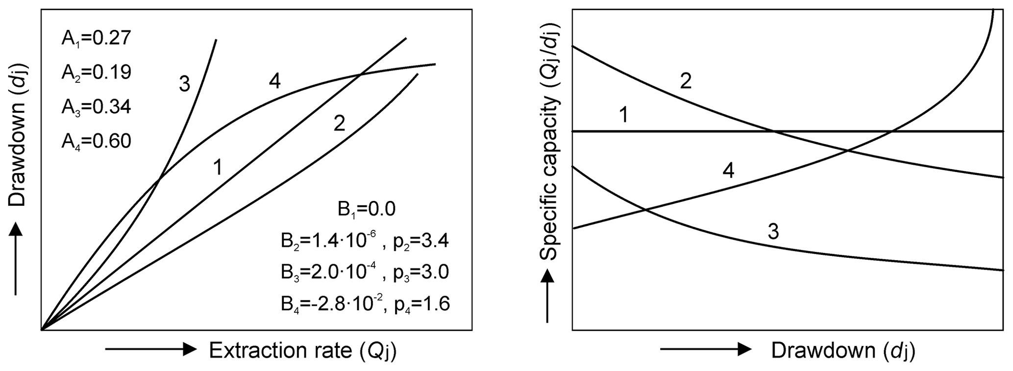
Figure 1Characteristic curves (adapted from Villanueva and Iglesias, 1984), where Aj, Bj, and pj are the Jacob equation coefficients. (1) Confined aquifer without head losses in the well. (2) Free aquifer without head losses in the well. (3) Aquifer with non-linear head losses. (4) Anomalous curve due to, following conventional criteria, poorly collected data or changing characteristics in an aquifer with pumping time.
In step-drawdown pumping tests, there is no unified criterion for the duration that each step should have. Thus, in contrast to the values used for the characteristic curves of these tests in some studies (Shapiro et al., 1998; Karami and Younger, 2002), in this study, it is considered that the steps must be performed for sufficiently long periods to have reached quasi-steady states. These states have been reached when the temporal variation of the drawdown is less than 1 % of the total drawdown for each step. This criterion has been adopted by considering its equivalence with the criterion established by Zha et al. (2017) on the temporal derivative of drawdown for quasi-steady state conditions and by considering the validity of assimilating the drawdown in the well to the average behaviour of the different levels in a multilayer aquifer.
A situation that is not often considered in studies on great continental detrital basins that are hundreds of metres deep is that the diverse permeable layers crossed by water wells can have different hydraulic heads. If this difference exists, then the permeability value determined for each permeable layer is incorrect, leading to an error in the estimation of the flow rate provided by each layer and causing a very important deviation in aquifer modelling. Although this possibility has been cited in several publications (Molz et al., 1994; Crowder, 2002; Le Borgne, 2006), no methodology has been published to quantify its effects in water wells in large continental detrital basins.
Flowmeter logging is conventionally used to determine variations in the flow velocity along a well casing, allowing water inputs at different depths that contribute to the total discharge rate to be computed. These quantities are used to estimate changes in hydraulic characteristics with depth, thereby improving the management and rational exploitation of aquifers. In addition to this conventional purpose, a process to provide information regarding different hydraulic heads in fractured rock media from flowmeter logs was proposed in several works by Paillet. Paillet (1998) showed the results of two flowmeter logs obtained with a heat-pulse flowmeter (lower limit of ∼0.1 l min−1 and upper limit of ∼20.0 l min−1) in Waupun (Wisconsin, USA). These flowmeter logs were measured under ambient and injection conditions at about 4 l min−1 and analysed for pumping or injection rates typically 1–5 l min−1. We think that the relationship used to estimate the transmissivity Tk of each fracture k, starting from the flow into the borehole qk, is , where a and b address the ambient and stressed conditions, respectively, wa,b are the water levels in the borehole for these conditions, R0 is the distance to the “outer edges” of the fracture, and rW is the borehole radius. This relationship does not depend on the unknown value of the far-field head in the aquifer Hk. Later, in Paillet (2000), is used to determine Tk. In this work “the results of high capacity tests, where the effects of ambient hydraulic-head differences would not be significant” were discussed. The hydraulic head values (4.54, 4.91, 4.91, 4.91, and 4.91 m below ground level) obtained for the four productive intervals found in one of the analysed boreholes are also presented in that work, although the process followed is not reflected in this paper. In Paillet (2000) the hydraulic head estimates (centimetres above open hole water level) in the same borehole (+28, −11, −11, and −11 cm above open hole water level) are shown. Based on this methodology, Day-Lewis et al. (2011) presented a computer program for flow-log analysis of single holes applicable up to 10 levels, in which the hydraulic head of each zone is determined by minimizing the differences between the flow rates obtained and those of the model and between the borehole's water level and far-field heads.
This communication presents the possibilities of the flowmeter log providing a hydrogeological explanation for the described anomalous cases. With this aim, in this work a method has been developed that uses flowmeter logs to provide information regarding different hydraulic heads in a multilayer basin. Determining these different hydraulic heads allows hydraulic reinterpretation that explains the abovementioned anomalous behaviours of the pumping test results.
To use flowmeter logs, a thorough pre-processing of results is necessary, without which the water inflow values determined in each filter can have very high errors and in turn allow an accurate determination of the head loss inside the well. Although different types of sensors have been used in well logging tools, spinner flowmeters are the most widely used in assessing the productivity of wells. Díaz-Curiel et al. (2020) proposed a complete reformulation for processing spinner flowmeter logs.
Another aspect related to the reliability of the flowmeter log results is the variability caused by differences in the near-wellbore or skin zone in the different layers of the well, for whose solution this work proposes the establishment of “flow stretches”. In this work, the term “flow stretch” is primarily used to differentiate sets of consecutive screens located at depths of the more permeable units (aquifers), among which there are other stretches mainly corresponding to less permeable units (aquitards). We have chosen to use the term “stretch” to avoid controversy with other terms such as “units”, which have a different hydrogeological meaning. Despite its origin, in this study, the term stretch is used to designate both the flow stretches in the well as well as the sets of layers to which they correspond. These stretches are obtained from a zonation process of the flowmeter log established by Díaz-Curiel et al. (1997), and it starts by generating a flow curve interpolated between water inputs. This curve is transformed into a smooth curve with constant depth increments. To obtain the depth values at which the limits between stretches are located, first the inflection points of the smooth curve are calculated and then the average values between those limits are determined. Finally, the upper and lower limits of each stretch of minimum values (the impermeable stretches) are approximated to each other, so that the average variance within each permeable stretch is minimal. These stretches show some parallelism with zonation relative to the average grain sizes shown in Díaz-Curiel et al. (1995), whose spatial extension is addressed in the discussion section. The use of the flow stretches allows the differences between screens within each stretch to be ignored, and their influence is not evaluated in this work because the average hydraulic conductivity of each flow stretch compensates for them.
Regarding the hydraulic interpretation of flowmeter logs, its main advantage lies in the fact that different permeable layers that the well crosses may have different hydraulic properties. These cannot be drawn from the results of a conventional pumping test without using packers. The differences are quantified by water inputs through screens corresponding to each layer and its thickness. In wells with a high technical control budget, the hydraulic characteristics of the different permeable layers can be achieved by using packers. However, despite the high cost of this technique in deep wells, the results do not have to match those obtained during operations with no packers on the pump. The main reason for this difference is that, at higher pumping rates, there is significant vertical flow through the gravel pack surrounding the screen (Boman et al., 1997). For example, for a well drilled to 44.5 cm and cased with a 39.2 cm filtering pipe (annulus space ∼ 1400 cm2) with a 2–3 mm gravel pack, the flow through it is larger than the water inflow through an isolated screen of 320 cm (area of ∼ 80 000 cm2) located in front of sands whose permeability is 100 lower. By isolating each layer, the static and dynamic water levels may be different from those presented in the well when all permeable layers are connected (“dynamic level” refers to the well water level when it reaches a quasi-steady state for a given pumping rate). The influence of pump depth is not analysed in this study, considering that it only affects the flowmeter logs mainly for measurements in front of the screens close to the pump and that the initial study depths are rather below the pump depth.
To achieve hydraulic interpretation from flowmeter logs, most authors (Molz et al., 1989; Rehfeldt et al., 1992; Ruud and Kabala, 1996; Zlotnik and Zurbuchen, 2003a; Barahona-Palomo, et al., 2011; Riva et al., 2012) start from the basis that hydraulic conductivity values for each permeable layer (from each screen) are proportional to the hydraulic conductivity of the entire well up to a multiplying constant. In these studies, the hydraulic conductivity is obtained from measurements by a nearby piezometer during pumping tests using the Theis equation (1935) between the discharge of a well and the water level drawdown a short distance from the well (Theis, 1963). That proportionality is a function of the ratio between the water input at each screen and the pumping rate and the ratio between the thickness of each screen and the saturated thickness of the aquifer. In mathematical form, the hydraulic conductivity value of the permeable layer j is given by (Kabala, 1994), where Qj is the water input at layer j, QP is the extraction rate of the well, b is the aquifer thickness, and KP is the hydraulic conductivity of the entire well. Among the different thicknesses in the literature, saturated thickness (Molz et al., 1989; Li et al., 2008), aquifer thickness (Clemo and Barrash, 2003; Riva et al., 2012), and screened casing thickness (Barahona-Palomo et al., 2011; Gueting et al., 2017) used to calculate the hydraulic conductivity of an entire well, the saturated thickness is employed in this work.
Unlike the previous procedure, this study follows the less common methodology established by Rehfeldt et al. (1989) starting from the Thiem equation (1906). Although there are contradictory opinions on the validity of this equation, some more recent studies consider that it is still applicable for determining the hydraulic characteristics of the well (Zlotnik and Zurbuchen, 2003b; Schneider and Attinger, 2008; Day-Lewis et al., 2011; Houben, 2015). Rehfeldt et al. (1989) stated that a unique radius of influence R0 value (the distance for which the produced drawdown in the aquifer water table is nil) allows the direct determination of the hydraulic characteristics of different permeable layers. Following the proposal in Rehfeldt et al. (1989), variation in the radius of influence can be neglected because it is included in the logarithm; therefore, its variation affects the hydraulic conductivity computation by less than 10 % for all permeable media in a given aquifer. This statement assumes that, for a certain type of aquifer, its radius of influence varies by only a few hundred metres around a mean value of approximately 1000 m (Villanueva and Iglesias, 1984).
For these reasons, the goal of this work is to investigate the causes of anomalies in the characteristic curves of pumping tests and to develop a methodology that improves the estimation of the hydraulic parameters in multilayered aquifers. Considering that the hydraulic conductivity (k) of the permeable layers should remain the same at different pumping rates, this advance is based on the fact that the hydraulic head of successive permeable stretches can be different, as already proposed by Bennett and Patten (1960). Although different hydraulic heads are acceptable for determining the hydraulic properties of fractured aquifers (Hess, 1986; Paillet, 2000; Lane, 2002), this is not conventionally taken into account in multilayered aquifers.
This methodology has been applied to a 475 m-deep borehole drilled in a multilayer detrital aquifer located in the centre of the Iberian Peninsula (Madrid basin). A step-drawdown pumping test was conducted in this well, showing discrepancies with Darcian behaviour and simultaneously with the non-Darcian coefficients of the Jacob equation. The relation between pumping rates and well drawdown in the step-drawdown pumping test as a whole did not show the expected behaviour for the type of aquifer considered. Moreover, the pump characteristic curves that were obtained do not correspond to any aquifer type. This difference results from the fact that the pumping rate increases with drawdown that has a power greater than 1 and that the specific obtained capacity increases with drawdown. A flowmeter log was collected, and the hydraulic interpretation is presented in this study, showing that the activation of the deepest aquifer stretches is the cause of this hydraulic behaviour, as explained throughout this study.
These results allow the avoidance of the possibly hazardous effects derived from intensive exploitation. As shown in this work, dangerously high arsenic contents occur in the deepest aquifer stretches in the Madrid basin (López-Vera, 2003). Since the studied well is part of the official network of the Madrid city water supply, it is imperative to limit the spread of this pollutant. As demonstrated by the hydraulic reinterpretation proposed in this paper, this aquifer undergoes strong activation when very high drawdown is applied, producing a sudden increase in its water inputs. This information is key to managing the exploitation network.
2.1 Estimating the hydraulic parameters
To determine the hydraulic conductivity K of the aquifer obtained through the entire well and each permeable layer, the Thiem solution (1906) is used, which is presented by Eq. (1) as a function of the radius of influence R0:
where Q is the extraction rate, b is the aquifer thickness, d is the drawdown in the well, and rw is the well radius.
The main drawback to this procedure, which is mentioned by Kruseman and Ridder (1970), is the influence of local well factors on the drawdown values. Excluding friction along the pipe (which depends on depth), the different local well factors that modify the obtained hydraulic conductivity of the permeable layers are (1) the reduction in the cross-sectional area of the well due to the submersible pump, (2) the entrance loss caused by flow through the screen slots, (3) the head loss due to the gravel pack, and (4) the head loss caused by the disturbed zone around the well (referred to as the skin effect) (Hufschmied, 1986; Rehfeldt et al., 1989). Some of these factors have been considered in detail regarding flowmeter logs (Ruud and Kabala, 1997; Ruud et al., 1999). In this work, these factors are not considered because they do not justify an increase or decrease in the hydraulic conductivity with depth; thus, although any of the four factors may have locally different values, their influence on the hydraulic conductivity obtained at each permeable level is constant for any flow.
As established by Rehfeldt et al. (1989), the hydraulic conductivity of each permeable layer is given by Eq. (2):
where qj is the water input produced in each screen, and Δzj is the thickness of each screen. Equation (2) has been applied in various studies (Xiang, 1995; Oberlander and Russell, 2006), but in this work, it is applied to well flow stretches.
2.2 Step-drawdown pumping test
In this type of pumping test, the hydraulic behaviour of the well is analysed through the characteristic relationship (Jacob, 1947) or in a more general form (Rorabaugh, 1953), as shown in Eq. (3):
where Q denotes the consecutive values of the extraction rate in each step, d is the corresponding stabilized drawdown (i.e. when its increase is negligible for an increase in the pumping time), A is a constant that depends on transmissivity, and B and p are fitting constants to the resulting data from the pumping test, where p is greater than 1 (Todd, 1980). The second term represents the apparent divergence from the linearity expected by Darcy's law (Darcy, 1856), which is addressed in Sect. 5. This is generally attributed to an increase in head loss due to turbulence as the pumping rate increases. It is also coherent when the dynamic level exceeds the depth of the upper aquifer layers, reducing the specific capacity. Although some authors consider that the Jacob equation (Eq. 3) can be improved, there are still authors who continue to use it (see Mathias and Todman, 2010).
The conventional interpretation of step-drawdown pumping tests begins with the fact that drawdown for different pumping rates is caused by either the general or extensive characteristics of the aquifer. In this way, confined, semi-confined, and unconfined aquifers are distinguished, whose curves, pumping rate versus drawdown, and specific capacity versus drawdown are different in each case (Fig. 1).
2.3 Flowmeter data processing method
The need for an exhaustive treatment of the flowmeter logs arose initially to rule out the possibility that the anomalies observed in the characteristic curves of the step-drawdown pumping test could stem from the reliability of the flowmeter log results themselves. Thus, it had to be shown that such anomalies were not due to head losses along the well. In addition, considering that the flow velocity used in the Darcy–Weisbach equation is raised to a power of 2, the differences between the head losses resulting from considering the actual flow velocity instead of the velocity directly measured by the sonde are greatly amplified.
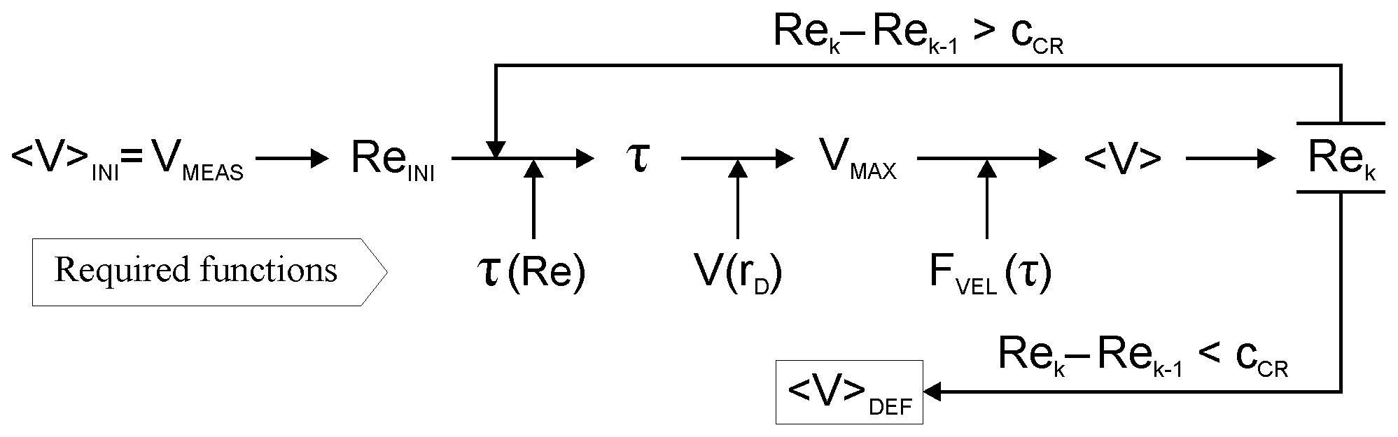
This exhaustive process of the flowmeter logs will be done according to the laws of pipe hydraulics using the methodology developed by Díaz-Curiel et al. (2020). To obtain the flow velocity at each depth, <V(z)>, a conventional iterative process is used. It begins by taking the measured velocity Vmeas at a given depth as the initial flow velocity and the initial Reynolds number Reini according to its definition, that is, , where ρ is the water density, D the well diameter, and µ the dynamic viscosity. Then, the relationship τ(Re) (see Eq. 4) that provides the flow turbulence exponent τ as a function of the Reynolds number is applied.
Knowing the turbulence exponent τ and the normalized radius rD of the sonde (the ratio of the sonde distance to the well axis with respect to the well radius), a velocity law must be applied. This law is the ratio between the velocity at the normalized distance V(rD) and the maximum velocity in the well axis Vmax (see Eq. 5); this allows this maximum value to be obtained.
Then, using the relationship for the velocity factor Fvel(τ), defined as the ratio between Vmax and the flow velocity <V> (see Eq. 6), the first flow velocity is obtained with the corresponding Reynolds number Reini, which is closer to the actual value.
Applying τ(Re), V(rD), and Fvel(τ), a new Re value Rek is obtained (k being the iteration index of the convergence algorithm). This process is repeated until a given convergence criterion is reached. The process schematic is summarized in the flowchart in Fig. 2 (adapted from Díaz-Curiel et al., 2020) to obtain Re(z).
In these equations, the influence of temperature is not considered because viscosity is practically homogeneous along the well due to water circulation during pumping.
Once the Reynolds number at each depth is known, the head loss can be obtained by the Darcy–Weisbach equation (Darcy, 1857; Weisbach, 1845) given by , where g is the gravity acceleration (m ⋅ s−2), <V> is the average flow velocity (m ⋅ s−1), D is the inner diameter of the well (m), ℓ is the length of each considered pipe element (m), and f is the friction factor (dimensionless) for smooth pipes given by Eq. (7):
It is important to point out that, according to Eq. (7), as in all pipe hydraulics relations, the friction factor decreases with the Reynolds number, except for the transition interval between laminar and turbulent regimes.
Applying the rigorous formulation presented to process the flowmeter logs (Eqs. 3 to 7) and considering that the sonde has a significant diameter (rD), the values of vary between 0.85 and 0.94. This difference represents a 20 % error in the total range of variation of that velocity ratio between 0.5 for laminar flow and 1.0 for fully turbulent flow. However, if the well diameter is smaller (close to the diameter of the sonde), V(rD) approaches Vmax, resulting in the ratio presenting a greater variation (from 0.50 to 0.83) for the range of Re found in the case studied than if the diameter of the well analysed is close to 0.2 m, as in the case studied in this work.
To estimate the hydraulic parameters from the flowmeter logs, once they have been processed, two specific approaches developed in this work are applied to obtain the actual hydraulic conductivity of the different layers. The first approach is to divide the well into flow stretches with different hydraulic behaviours as a function of the flowmeter results. The second approach is based on the fact that the hydraulic head of the deepest flow stretches of the well do not necessarily match the head of the overall well (Fig. 3).
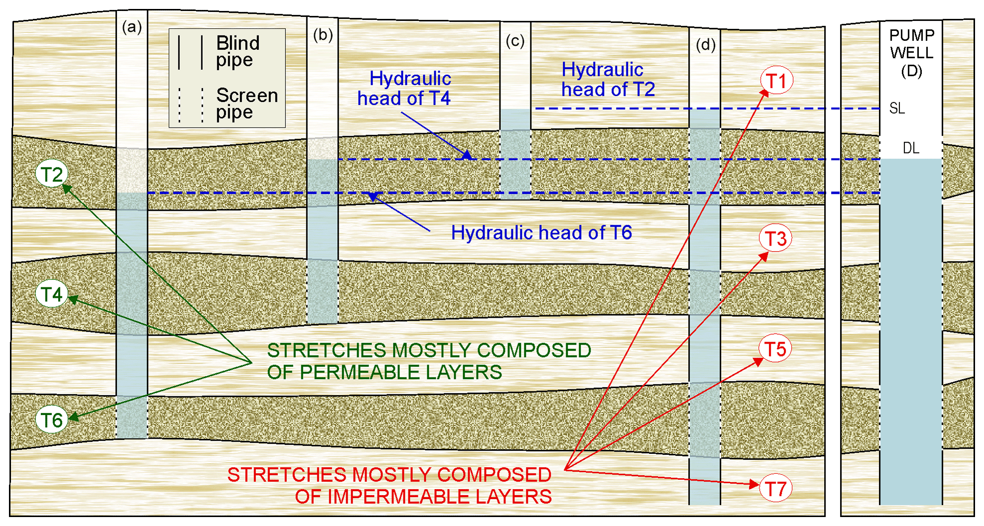
Figure 3Hypothetical example of the results that would be obtained in a large detrital basin composed of seven different stretches so that permeable stretches T2, T4, and T6 would be hydraulically separated from each other by impermeable stretches T1, T3, T5, and T7; stretches T2, T4, and T6 would have different hydraulic heads, which are drawn in hypothetical wells A, B, C, and D, with different depths and different filtering intervals. Considering the plotted depth and filter intervals of well D, if pumped with the plotted dynamic level DL (coincident with the hydraulic head of T4; see the right part of the figure), only the T2 stretch contributes water to the well, T4 does not, and T6 collects water from the well. Note that the well diameters plotted are not scaled but are highly magnified to enhance the view of the figure.
The hydraulic head of a flow stretch is defined as its effective static level, that is, the height of the water level that would be achieved if the well were connected with the aquifer only through this stretch. This work proposes that a flowmeter log allows us to know the existence of hydraulic heads that are different for each stretch. This distinction implies changes in the effective drawdown of each stretch, which justifies, as shown in the case study, the water inputs of the deeper aquifer stretches not being proportional to drawdown.
In most works on hydraulic interpretation of flowmeter logs, a unique hydraulic head given by the static level HSL of the entire well is considered (Molz et al., 1989; Rehfeldt et al., 1992; Ruud and Kabala, 1996; Zlotnik and Zurbuchen, 2003a; Barahona-Palomo, et al., 2011; Riva et al., 2012). Thus, the drawdown used in the Thiem (1906) equation is the same for all of the aquifer stretches in a well, , where hDL(s) is the dynamic level for the “s” pumping step and HSL is the dynamic level of the entire well. However, under the hypothesis presented in this work, the hydraulic head of each stretch, and therefore the corresponding drawdown, can be different. Numerically, the drawdown of each flow stretch TN will be given by the following relation:
where hSL(n) is the static level for flow stretch TN. In short, the proposed method consists of replacing the single drawdown d in Eq. (2) from Rehfeldt with a drawdown for each stretch.
The main differences with the method used by Paillet (1998) are that we have chosen to use the Rehfeldt relationship (Eq. 2) for permeability instead of the Davis and DeWiest relationship (1966) relation for transmissivity, given that the thicknesses of the layers and the productive sections are taken into account. The advantage of this option is that it is not necessary to know the storage coefficient of each contribution interval studied. It has also been considered that the different hydraulic heads are below the static water level (the water level in ambient conditions from Paillet, 1998). The procedure developed is based on the linearity of the hydraulic behaviour of the aquifer sections, and each section is treated separately.
The proposed method for obtaining the hydraulic head of each flow stretch is to (1) correct the drawdown values of the total head loss due to flow along the pipeline and (2) modify the height of the hydraulic head for each flow stretch until the straight line fitted to the data, qN(s) versus dN(s), reaches the maximum regression coefficient (where qN(s) is the water input in flow stretch N for the s pumping steps). With a static level value for each flow stretch, the effective drawdown of each flow stretch can be obtained, and although other local well factors may cause differences between screens within each stretch, their influence is not evaluated in this work because the average hydraulic conductivity of each flow stretch compensates for them.
4.1 Geology of the area and well characteristics
The study well (named CNC in this work) is located in the Tagus River basin in the Iberian Peninsula. More specifically, it is located in the western sub-basin, also known as the Madrid basin, near the city of Madrid (Spain). The Madrid basin has a triangular shape and is bound by several mountain ranges, the “Central System” of the Iberian Peninsula of igneous–metamorphic nature, located north-west of the Madrid basin and the main contributing source area (Fig. 4). The structure of the basement corresponds to that of a complex graben and has resulted in a sediment thickness of approximately 1000 m, although in some areas, the thickness can exceed 3000 m. The Tertiary (Miocene) sediments that fill the basin correspond to continental deposits of an arid, endorheic nature that are fed by alluvial fans; these alluvial fans develop edge or detrital facies, intermediate or transitional facies, and central facies, all of which are characteristic of this depositional system (Navarro et al., 1993).

Figure 4Geological map of the Madrid region (adapted from Diagnóstico Ambiental de la Comunidad de Madrid, 2020) with the studied well location and location of the schematic cross sections shown in Fig. 11.
The aquifer is located in the continental siliciclastic basin of Madrid, which in the literature is separated into two lithostratigraphic formations differentiated by grain size and, therefore, by hydrogeological characteristics; due to the depositional process of the materials, they are differentiated from one area to another as well as vertically. The lower formation is composed of arkose that is generally very clayey with clayey sand. The upper formation consists of arkosic coarse-grained sand, gravel, and clay. Although the upper formation is sandier and permeable and overlaps the more clayey lower formation, they are not considered different aquifers (López-Vera, 1985) but rather a heterogeneous and anisotropic free aquifer system where more permeable layers are separated by clayey strata with a lower permeability (which qualifies as a multilayer aquifer).
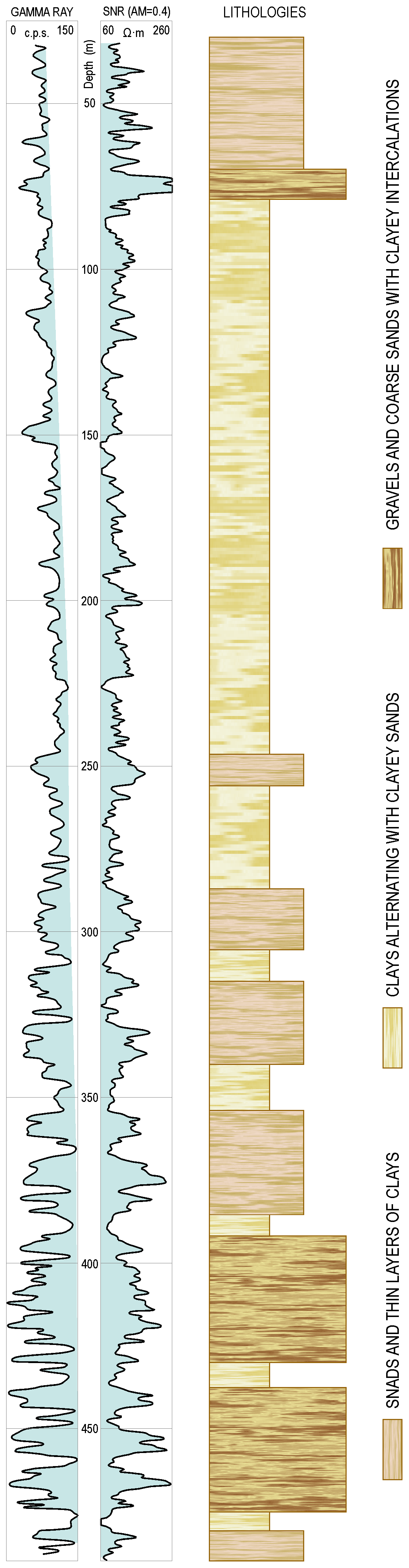
A lithological column was compiled from information provided by the detritus from the borehole and conventional well logs: normal resistivity and natural gamma ray logs, which are presented in Fig. 5. Note that the logs were not corrected for borehole diameter, conductivity, or mud density; therefore, there was a notable difference between the larger diameters in the upper part and the base. Three differentiated parts were established: the first (0 to 75 m) was composed of sands alternating with thin layers of clay, the second (75 to 285 m) comprised alternating sandy clay and thin sandy layers, and the third (285 to 485 m) had a predominance of coarse sand and gravel with intercalations of very thick clay layers. As a result of the correlation between lithological stretches in the north-western zone of the studied basin (Díaz-Curiel et al., 1995), the permeable stretches can be considered radially homogeneous differentiated aquifers. With the exception of the superficial part, the rest of the permeable stretches can be treated as confined aquifers. This allows the use of the Thiem equation for these stretches and for obtaining hydraulic parameters on a regional scale (as proposed by Rehfeldt) by averaging the stretches as a whole (Sánchez-Vila, 2006).
The borehole was rotary drilled with a diameter of 660 mm down to a depth of 120 m, and then it was drilled with reverse injection of natural mud with a diameter of 445 mm to a final depth of 490 m. The construction details of the well consisted of casing to a depth of 480 m, with a 404 mm inner diameter in the sections of blind pipe and 392 mm in the wire-wrap screen sections; a gravel packing of 2–3 mm grains was added throughout its length. The well was developed by adding previously diluted polyphosphates, and after 12 h, a series of intermittent pumping was carried out; once the extracted water contained no suspended fines, a 72 h gauging of increasing pumping was conducted up to a flow rate of 100 l s−1.
4.2 Pumping test results
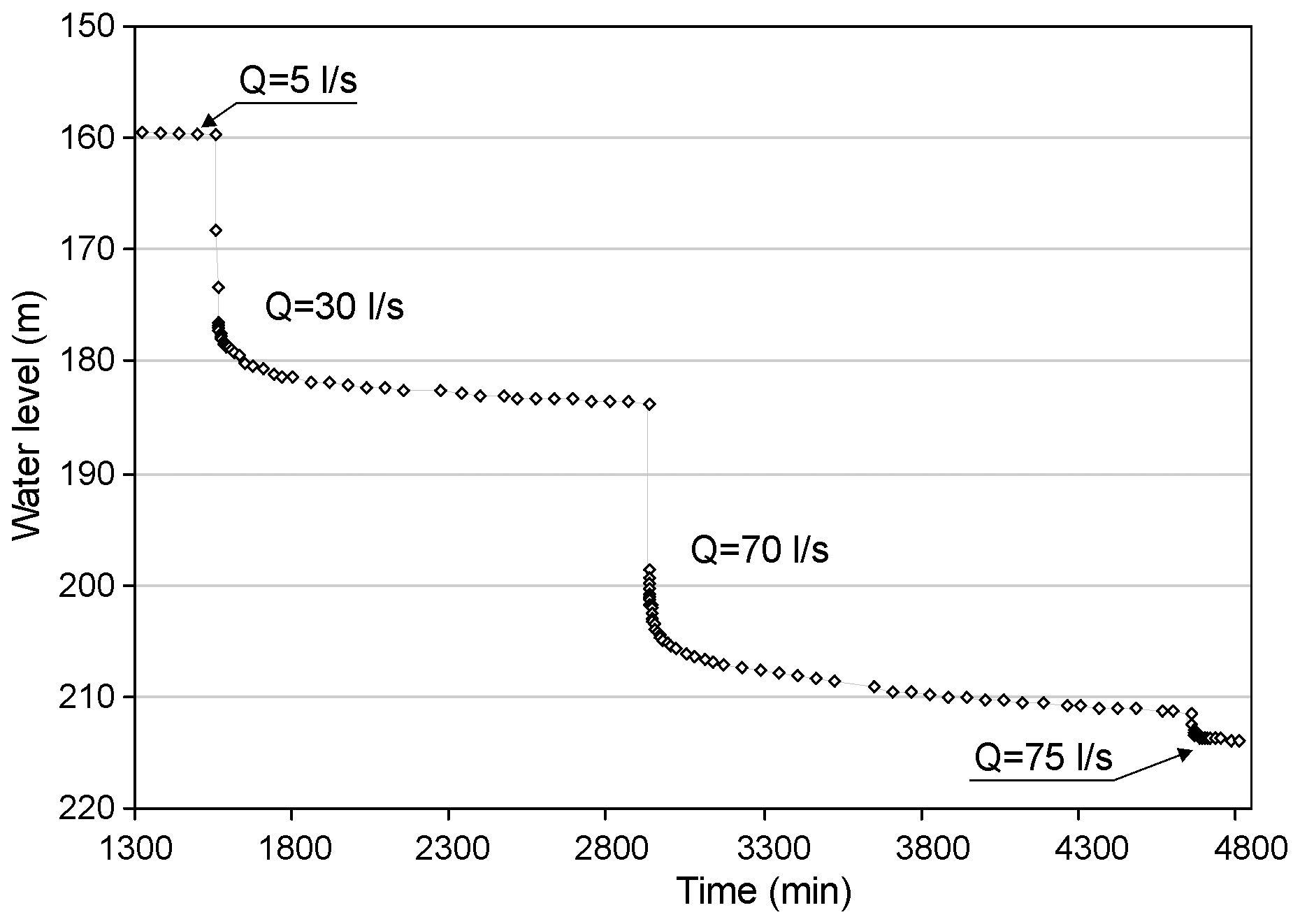
After a process was conducted to eliminate the well storage effect, the static level settled at a depth of 151 m. The pumping test started with a flow of 5 l s−1 until the hydraulic head stabilized. Two main extraction pumping rates of 30 and 70 l s−1 and a final rate of 75 l s−1 were then used, with a total elapsed time of 80.5 h. All steps were performed for a sufficient time to reach the quasi-steady conditions mentioned in Sect. 1. The resulting temporary data are shown in Fig. 6, and the drawdown values for each pumping rate are shown in Table 1.
Hydraulic conductivity values were obtained using Eq. (1) (Thiem, 1906), taking the saturated thickness to be equal to 329 m (the depth of the well minus the depth of the static level) and considering a radius of influence of 950 m once the quasi-steady state was reached. This last datum is the central value of those shown in Villanueva and Iglesias (1984) for semi-confined and confined aquifers. The resulting hydraulic conductivity values of the well are shown in Table 1, and they increase with drawdown.
Table 1Pumping test results in the case study.
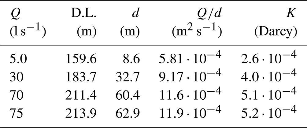
Q: pumping rate. D.L.: dynamic level. d: drawdown. K: hydraulic conductivity.
The hydraulic conductivity values that were obtained do not have to coincide with the general values of the aquifer (since the general values of the well also depend on the construction details) or with those obtained for each of the different permeable stretches that the well crosses (since the result for the well is an average behaviour of those flow stretches). However, it is possible to speak of a mean value (geometric average) of approximately Darcy. To hydraulically characterize the well from the pumping test results, Fig. 7 shows the pumping rate versus drawdown Q(d) and the specific capacity versus drawdown .
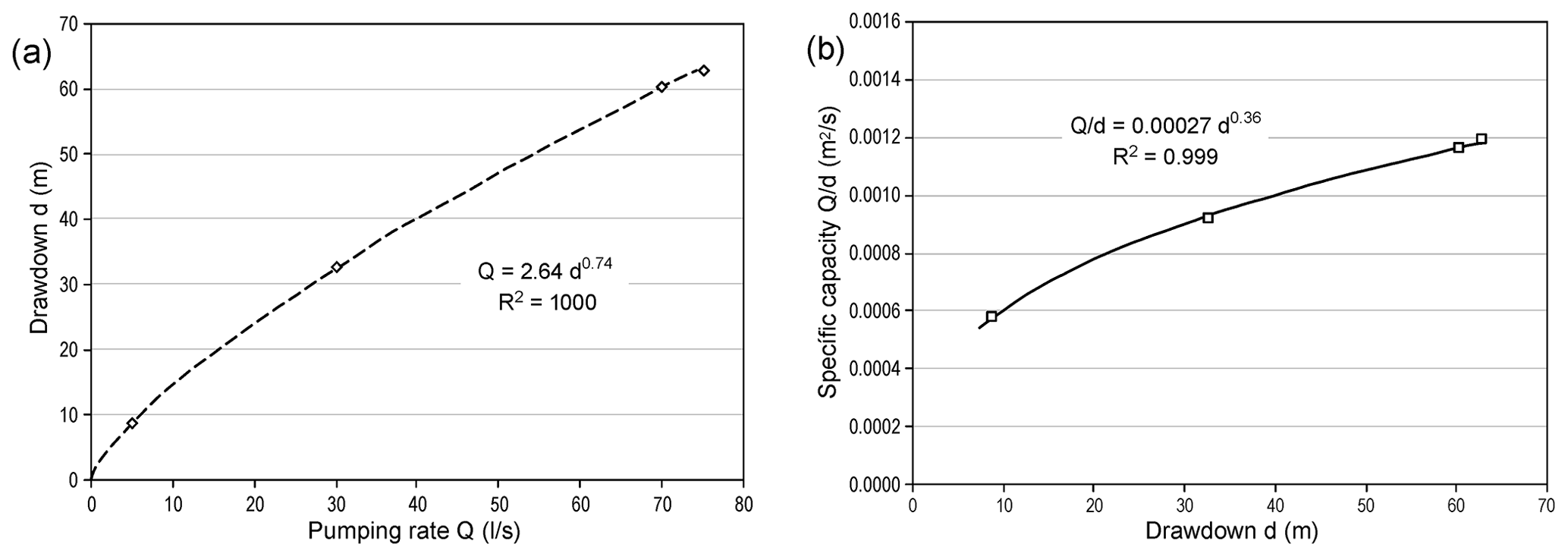
Figure 7(a) Drawdown versus the pumping rate (b) and the specific capacity versus drawdown in the case study.
Let us remember that in the characteristic equation for the well for step-drawdown pumping tests, the first term corresponds directly to Darcy's law (1856) for the total volume of the water flow crossing through successive cylindrical layers. In the second term, the exponent p can be greater than 1; successive drawdown should show a power relationship with an exponent greater than 1 versus the pumping rate. Moreover, the specific capacity should decrease with successive drawdown; otherwise, the well extraction ratio would increase with drawdown. However, in Fig. 7, the opposite pattern is observed; i.e. d(Q) increases with a power that is less than 1, and increases with drawdown. These anomalies do not seem to arise from errors in the water level measurement, as their values versus time appear to be correct (Fig. 6).
4.3 Flowmeter results
The static level HSL was measured at a depth of 157 m before the beginning of flowmeter logging. Flowmeter logs were obtained for pumping rates of 20 l s−1 (measured dynamic level at 172 m), 30 l s−1 (dynamic level at 178 m), and 70 l s−1 (dynamic level at 205 m). The drawdowns of the entire well for each pumping rate, without including the head losses, hence are 15 m, 21 and 58 for 20 l s−1, 30, and 70, respectively.
Since the flowmeter logs (spinner type) were collected during pumping operations, measurements could be obtained only below the pump depth. For the pump located at a depth of 191 m, logs were recorded from 200 to 470 m for pumping rates of 20 and 30 l s−1, and for the pump located at 253 m, logs were recorded from 260 to 470 m for pumping rates of 30 and 70 l s−1. The logs were obtained with an average sampling rate of 33 cm. Once calibration has been applied, the velocity obtained is averaged from the top of each screen to the bottom of the next, obtaining the values at 40 depths that appear in the raw data.
Equation (5), that of , used a normalized distance of 0.64, which corresponds to the ratio (, where rs is the external radius of the spinner frame (the sonde has a device that maintains its hold on the wall) and rw is the inner radius of the well casing. The different diameters (difference < 1 %) in the screens were not considered due to the difficulty of executing the iterative process to obtain <V>. The initial velocity values considered in the iterative process were obtained by applying the calibration curve to the velocities measured by the sonde. The initial Re values varied between 860 and 211 000 for all flow rates and pumping rates. For τ(Re), Eq. (4), the resulting values of the turbulence exponent varied from 1.0 to 6.7, resulting in values of between 0.85 and 0.94. The velocity factor values determined using Eq. (6) were in the range of 0.50 to 0.83, and deviations with respect to the average value reached 35 %. In addition to the zone where the studied well is located, there is no geothermalism at all, and the influence of temperature is not considered, as in the common equations on the hydraulic characterization of aquifers.
Figure 8 shows the results obtained for the main parameters and ratios of processing flowmeter logs by applying the methodology of Díaz-Curiel et al. (2020).
The accuracy of the measuring equipment was 0.5 l s−1, which greatly reduced the reliability of the results between consecutive screens and produced strong variation in the quantified water inputs from each screen.
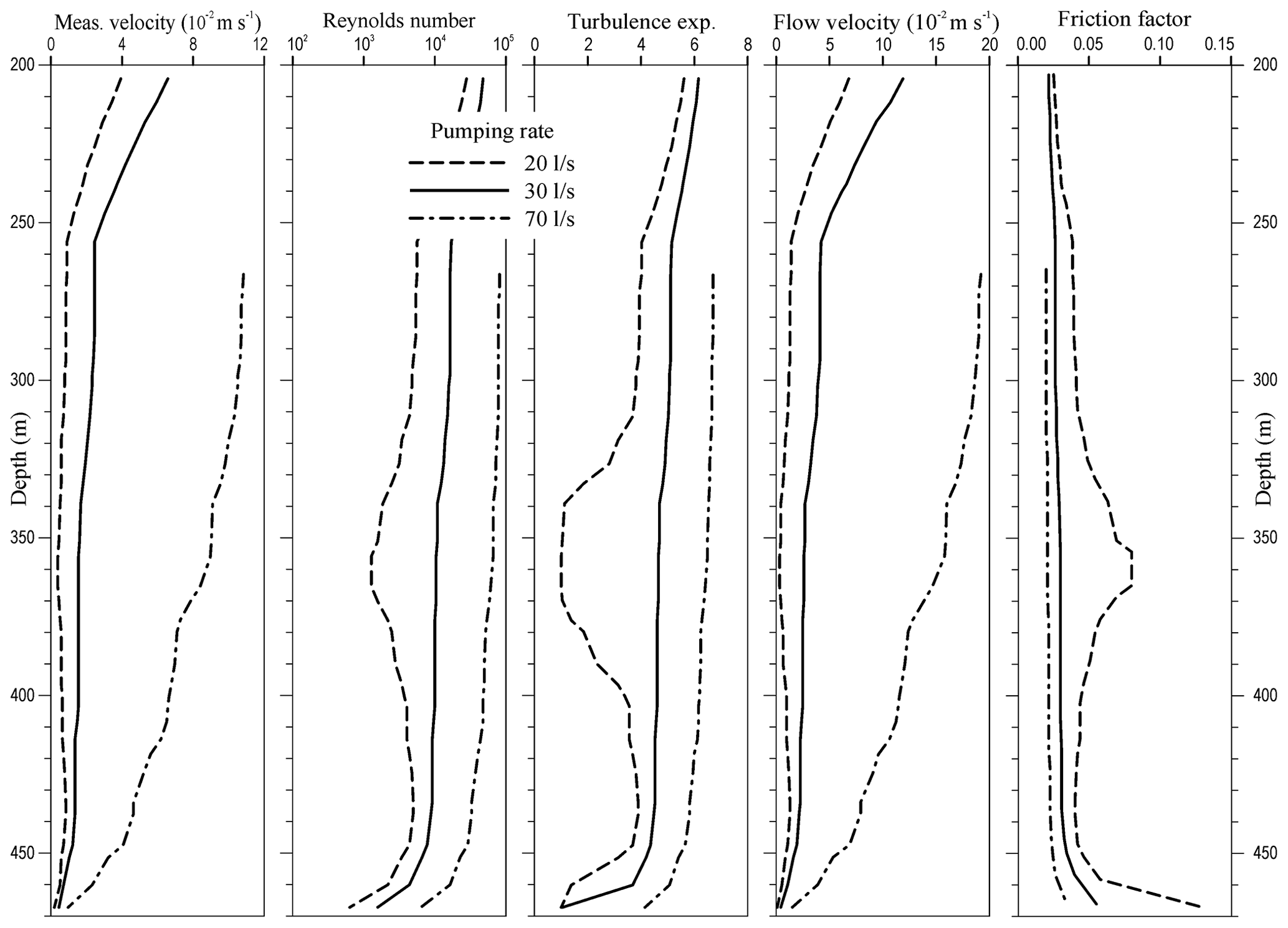
Figure 8Results obtained for the main parameters in the case study and the calculated friction factors (Díaz-Curiel et al., 2020).
4.4 Head loss results
The head loss was calculated using the Darcy–Weisbach equation (Darcy, 1857; Weisbach, 1845), and the friction factor was calculated using Eq. (7). The curve of the friction factor values obtained for pumping rates of 20, 30, and 70 l s−1 is shown in Fig. 8. Depending on the scale on which the transition interval is analysed, the turbulence of the fluid flow cannot be determined at all points along its path. In this study, we chose to use a fitting expression for smooth pipes given by Eq. (7) because the flowmeter sondes used in well logging reflect the fluid advance on a much larger scale. The friction factor for low pumping rates in the deep screens increased by a maximum of 70 % compared to that obtained using conventional equations.
The total head loss below the pump is obtained by integrating the head loss throughout the well based on the flow velocity obtained at each depth (see Fig. 8); that is, the cumulated Δh adding the successive local head loses values relying upon local friction factors and local water velocities. Above the pump depth, the calculation is based on a linear increase in the velocity between the pump depth and the dynamic level. The obtained values of the head loss Δh(s) for each pumping rate are shown in Table 2, which will be used in the calculation of the effective drawdown produced.
Table 2Head loss values for each pumping rate in the case study.
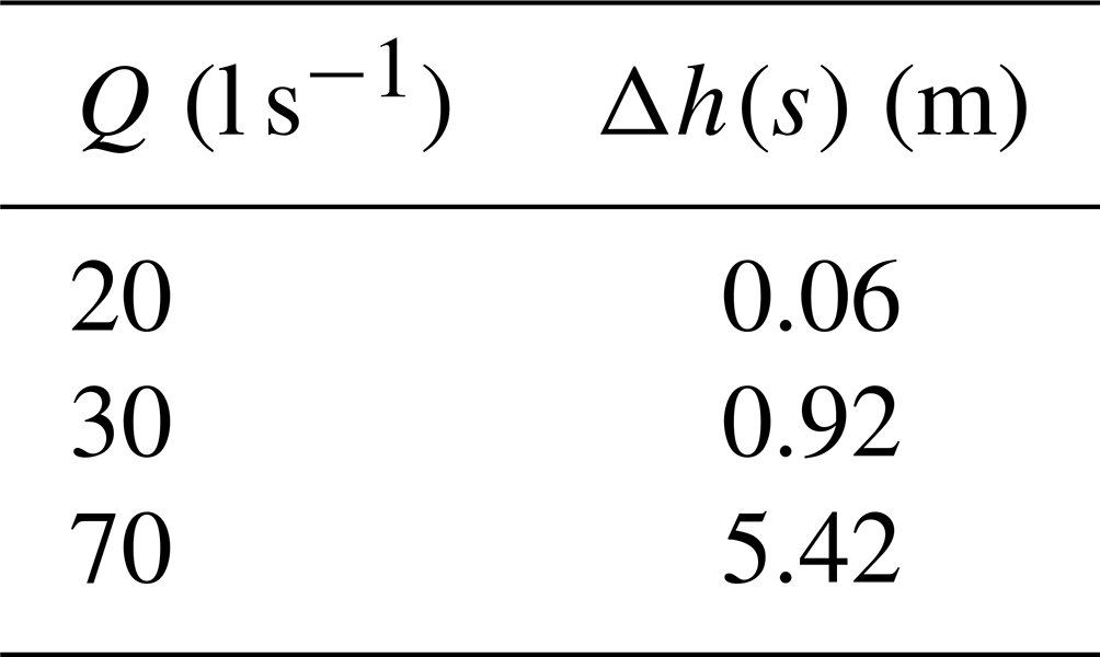
In this case, the friction factor reaches values 6 times higher at the bottom of the well than at the initially recorded depth, and the value of the head loss is low (0.06 m), because the average velocity in the Darcy–Weisbach equation is raised to a power of 2. Therefore, in large-diameter water wells, the influence of the friction factor along the pipeline is negligible. Finally, despite the inclusion of head loss values, the water inputs from some of the stretches still do not maintain the expected proportionality with drawdown, so hydraulic reinterpretation is carried out using the flowmeter results.
4.5 Water inputs
Figure 9 shows the results from different pumping rates after processing. On the left-hand side of Fig. 9a, the curves for upward flow rates versus depth are shown, and in Fig. 9b, the water inputs deducted in the different screens are shown, while the negative water inputs (outputs) are not shown in Fig. 9b.
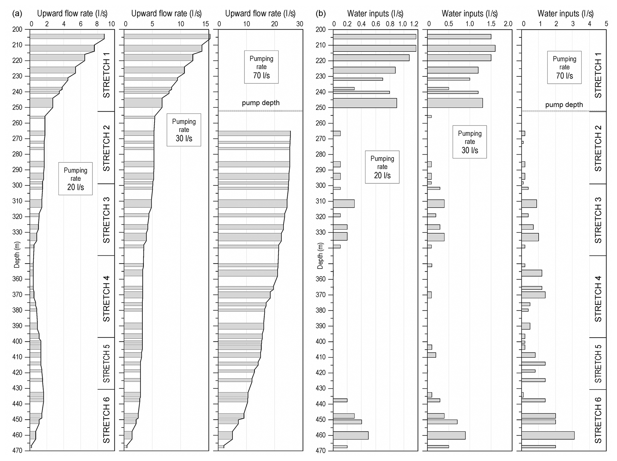
Figure 9Flowmeter results in the case study (grey horizontal bars reflect the depth intervals of each screen). (a) Upward flow rate versus depth; (b) water inputs from each screen.
Note that the accuracy provided by the equipment is 0.05 l s−1, which greatly reduces the reliability of the results between consecutive screens and produces strong variations in quantifying the water inputs from each screen. For this reason, following the criteria described in Sect. 3, the flowmeter log is divided into different flow stretches based on the average productivity of each flow stretch.
Table 3 shows the water inputs from the different flow stretches for each measured depth interval. A “top” stretch has been added to the top of the well above the pumping depth, where the different water inputs are unknown. The water input in the upper part (which includes flow stretch T1 for the case of a pumping rate of 70 l s−1) is obtained by the difference between the pumping rate and the deduced flow rate at that depth.
At a pumping rate of 70 l s−1, the water input from flow stretch T1 is not known, and the input of this flow stretch may increase in proportion to the pumping rate, which should imply that the upper part of the well would remain constant (e.g. due to the dynamic level dropping below some of the upper layers).
Both Fig. 9 and Table 3 show that the water input from flow stretch T2 is very low, even for high pumping rates, and it is close to the flowmeter accuracy; hence, that flow stretch is omitted from the analysis.
Table 3 shows that for pumping rates of 20 and 30 l s−1, the water inputs from the upper part of the well and from flow stretches T1, T3, and T6 increase in a way that is practically proportional to the flow (with a ratio ≈1.5) and fits a confined aquifer. Flow stretches T4 and T5 have negligible water inputs, reaching negative inputs for a pumping rate of 20 l s−1. However, for the 70 l s−1 pumping rate, there is an abrupt change in the hydraulic behaviour of the well. On the one hand, the whole water input from the upper part of the well and from flow stretch T1 does not increase proportionally to the pumping rate (ratio = 2.33). On the other hand, flow stretch T6 shows a sharp increase in the water inputs, and flow stretches T4 and T5 present an apparent activation. Given the possibility that an increase in the head loss could justify such behaviour, values for each pumping rate were calculated and added.
The high correlation of the water inflows in stretches 2 and 3 for the pump located at the depths of 191 and at 253 m confirms the consideration that the depth of the pump does not affect the values obtained with the flowmeter logs.
Table 3Water inputs of flow stretches for different pumping rates and fractions over the total flow rate QT in the case study.
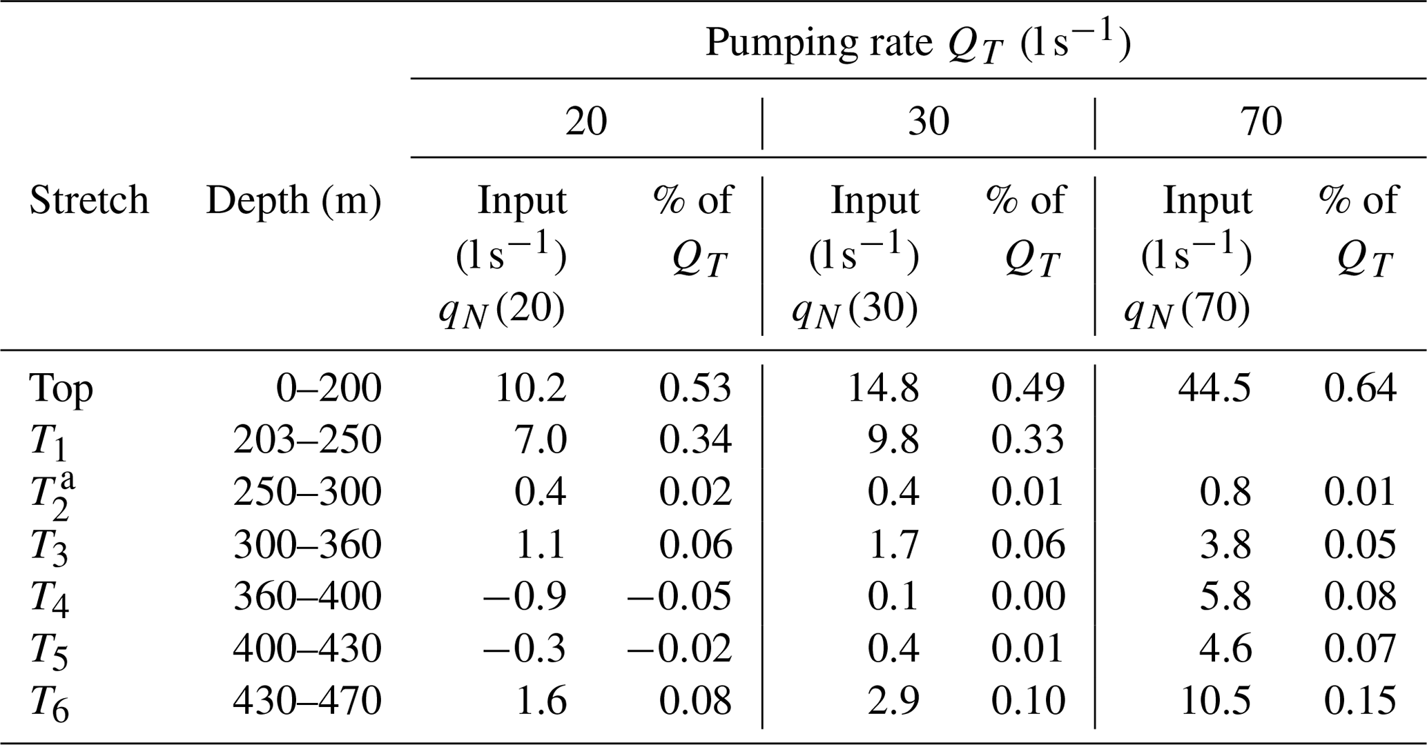
a As cited above, this flow stretch is not analysed because its water inputs are very low for all pumping rates.
Regarding the existence of different hydraulic heads, note that the negative water input in flow stretches T4 and T5 for the pumping rate of 20 l s−1 corroborates the validity of the hypothesis in this work. These negative inputs reflect the fact that when the drawdown is located above the hydraulic head of these flow stretches, the water flow does not occur inwards towards the well but rather outwards, reducing the upward vertical flow. In any case, the fact that the deeper flow stretches have a hydraulic head below the static level of the well explains why the pumping rate versus drawdown curve adjusts to a power function with an exponent greater than 1, and the specific capacity versus the drawdown curve is ascending. There are several studies in the literature that mention negative water inputs as those obtained in this case, but they do not present the hydraulic interpretation thereof; most of them correspond to flow logs measured in ambient conditions (Paillet et al., 2000; Butler et al., 2009; Day-Lewis et al., 2011).
4.6 Hydraulic reinterpretation
The permeability of each stretch has been calculated using Eq. (2). Instead of the contribution of each layer qj, the sum total of the contributions of each stretch qN(s) is considered (see Table 3). The unique initial drawdown d considered in Eq. (2) has been modified by the drawdown of the entire well for each pumping rate (s) (Δh(s) being the head losses shown in Table 2). The static level HSL is 157 m (as determined before the flowmeter logging was conducted) and the dynamic levels hDL(s) are 172 m for a pumping rate of 20 l s−1, 178 m for a pumping rate of 30 l s−1, and 205 m for a pumping rate of 70 l s−1. The thickness of each layer Δzj has been replaced by the thickness of each stretch Δz(TN) (depth intervals in Table 3). The radius of influence (R0) considered is 950 m (as in the previous calculations), and the well radius (rw) is m. The characteristic curves of each stretch are shown in Fig. 10a.
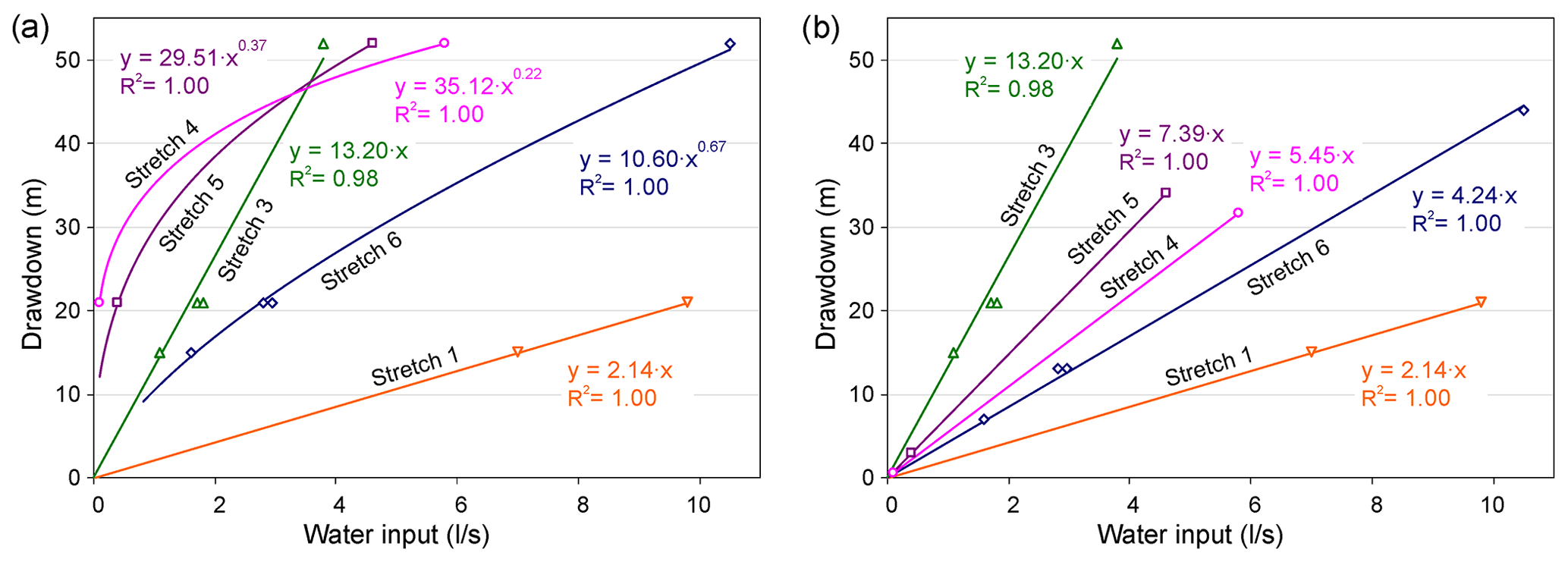
Figure 10Drawdown versus water inputs for different flow stretches in the case study. (a) dN(s) # qN(s) with a unique hydraulic head for all the stretches. (b) dN(s) # qN(s) with the modified hydraulic heads for each stretch obtained considering that p is at least equal to 1 in the Rorabough equation.
Analysing the specific capacities of different flow stretches, T1 and T3 show the expected proportionality for a confined aquifer. However, this is not the case for flow stretches T4, T5, and T6, whose dN(s) versus qN(s) data fit to a power function with exponents of 0.22, 0.37, and 0.67, respectively (see Fig. 10a). Not only does this not reflect Darcian behaviour, but it also indicates an exponent p in the Jacob equation of less than 1, as is the case with the well as a whole (see Fig. 7).
However, if it is considered that flow stretches T4, T5, and T6 have different hydraulic heads, the results vary. Through an iterative process, the value of the static level (hydraulic head) of each flow stretch for which the total water input of the flow stretch versus the drawdown acquires greater alignment can be determined. This means that when the data are fitted to a straight line, the regression coefficient is maximum. In other words, the resulting exponent in the Jacob equation when the data are fitted to a power function is p=1. Thus, for flow stretch T6, the static level for which inputs versus drawdown acquire greater alignment occurs at a depth of 165 m. Similarly, the resulting static level for flow stretch T5 is located at a depth of 175 m. For a pumping rate of 70 l s−1, flow stretch T4 undergoes an “activation” effect (even higher than flow stretch T5) when the dynamic level exceeds the true static level of T4, which is computed at a depth of 177.5 m. In summary, the hydraulic heads hSL(N) obtained with this criterion are 157 m for T1 and T3, 177.5 m for T4, 175 m for T5, and 165 m for T6.
Figure 10b shows the regression lines of water inputs versus drawdown for each stretch, with the corresponding relationships and R2 coefficients.
With these differentiated static levels, the hydraulic conductivities of each flow stretch were obtained using a next change of Eq. (2) (Rehfeldt et al., 1989) replacing d0(s) with , whose values are presented in Table 4.
The successive relationships used to arrive at the actual permeability with depth have been
It must be pointed out that kN is the same for the different (s) because the ratio is the same for any pumping rate (dN(s) versus qN(s) are fitted to a straight line).
Table 4Specific capacities and permeabilities of flow stretches for the static level determined in the case study.
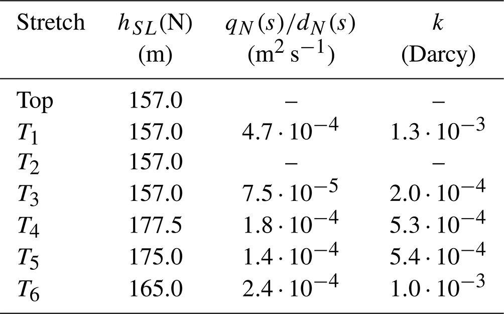
The average hydraulic conductivities of the stretches in the studied part of the well (200 to 470 m) have values between and Darcy, providing a geometric mean value of Darcy, which is close to the average hydraulic conductivity obtained with the pumping tests. The largest contrast occurs with the difference between the hydraulic conductivity values of the different flow stretches, which is close to an order of magnitude.
As mentioned at the beginning of Sect. 4, the precision of flowmeter logs does not allow us to obtain reliable hydraulic conductivity values of each permeable layer to make a more detailed characterization of each stretch. However, that analysis could be undertaken by considering the average water input and average thickness.
Regarding the linearity predicted by Darcy's law, in this work, the variation corresponding to non-linear flow is a different process than the change in the flow from a laminar to turbulent regime. Takhanov (2011) determined that the onset of non-linear flow occurs prior to the change to turbulent flow; in fact, some authors have considered that turbulent flow does not occur in porous fine-grained media in their natural state (Green and Duwez, 1951; Bakhmeteff and Feodoroff, 1937). In this sense, Houben (2015) established a linear laminar regime in the aquifer that becomes non-linear in the gravel pack and only becomes turbulent on the screen and inside the pipe. In this work, the regime change is less gradual than that predicted by the Forchheimer equation (1901) and does not increase with the same power after the transition. It should be taken into account that both the values of the friction factor and the particle Reynolds number established for the Forchheimer flow decrease as Re increases. To analyse the flow linearity in water wells, the hydraulic characteristics of the flow in the aquifer levels must be quantifiable by the velocity near the well. Moreover, a value of 0.01 m s−1 can be considered the maximum velocity in groundwater near wells. For example, if a water well with a very high extraction rate of 100 l s−1, radius of 0.2 m, total length of 400 m, and screened length of 80 m (20 %) is considered, then the average water input velocity would be 0.005 m s−1. Considering the results in van Lopik et al. (2017), non-linear behaviour starts at velocities greater than 0.01 m s−1, so the maximum water input still exhibits Darcian behaviour.
Among the possible explanations for the difference in hydraulic head values for the deeper flow stretches are hydrogeological reasons, such as the presence of flow stretches with different vertical transmissivities. However, the approximated values for the hydraulic conductivity in the less permeable stretches (T2 and T4) contradict this hypothesis, since flow stretch T2 is less permeable than flow stretch T4, but flow stretch T3 is not affected by a similar effect. Another possible explanation is that the change in the effective drawdown is due to the existence of nearby extraction wells, which overexploited the aquifers corresponding to flow stretches T4 and T5, thereby producing a drop in the static level of these flow stretches.
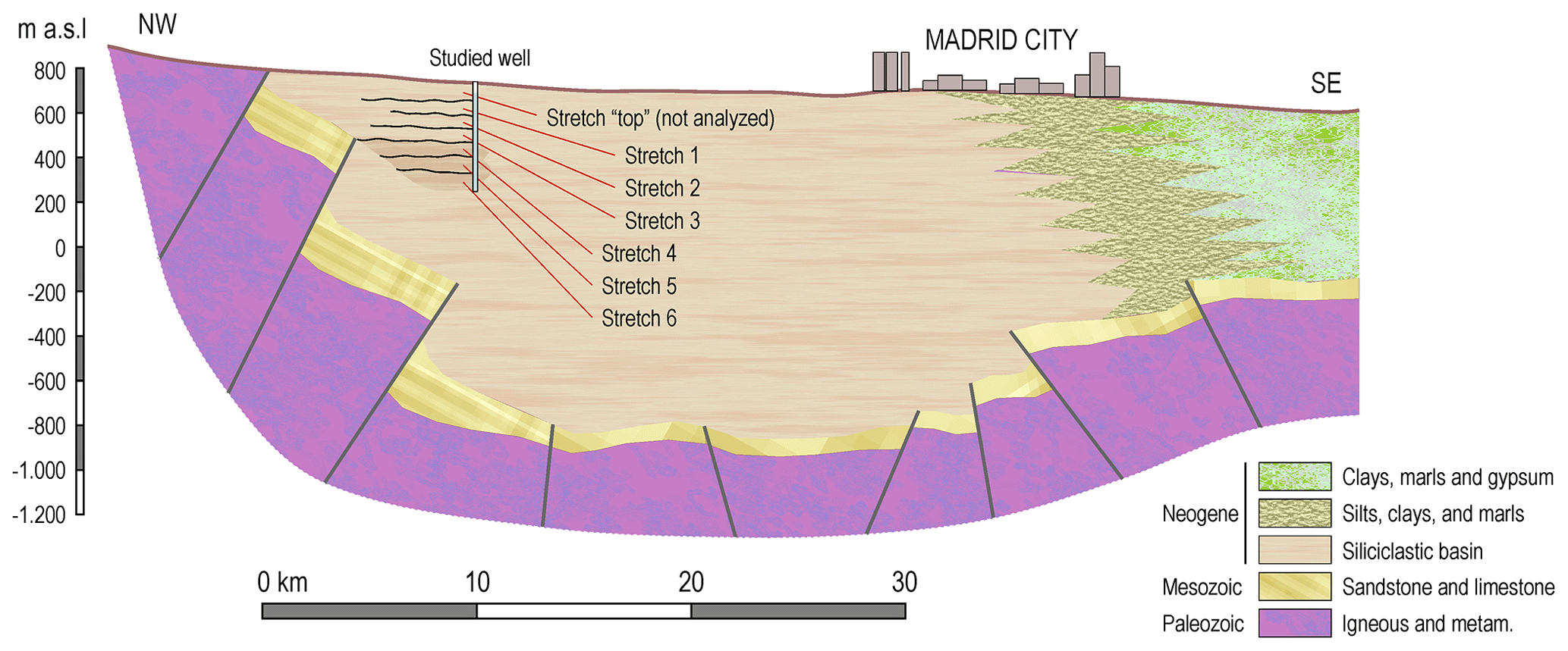
Figure 11Schematic geologic section of the Madrid basin (adapted from Llamas, 1976, and Navarro et al., 1993) with stretches established in the studied well.
Concerning the reliability of the final permeability values, one aspect that must be considered in estimating hydraulic parameters from flowmeter results is that the analysis was conventionally performed through the screens assembled in the casing. However, the distribution of these screens only approximately matches the permeable layers that the well crosses. Hence, differences between the thicknesses of the permeable layers and the assembled screens may exist as well as permeable layers that are not faced with a screen, whose effects are minimized by gravel packing. This effect adds to that produced by the local factors of the aforementioned well, which is an additional reason for differences in the water inputs of the different screens within each stretch.
Therefore, although the results of the pumping tests and the flowmeter results yield a similar hydraulic conductivity value for the entire well, after considering the possible hydraulic head difference that justifies and relates the anomalies reported over the pumping test data, this value moves away from the actual hydraulic conductivity of the aquifer.
Under the consideration that vertically there is a high hydraulic connection (similar to the horizontal one), it is common practice in hydrogeology to model large aquifers as an equivalent porous medium. In addition to obtaining water balance results, such models have a wide application in many basins (De Filippis et al., 2016). However, this study focuses on a case where the vertical hydraulic connection is much lower than the horizontal one, as can be deduced from the existence of the different hydraulic heads found. In this study, it is considered that the low hydraulic connection due to the existence of one or several wells in a basin of the size studied does not significantly affect the lateral variations of the hydraulic head along the basin. In contrast with several works taking into account the hydraulic head field (Yeh et al., 1996; Axness and Carrera, 1999), in this study it is considered a single hydraulic head for distances smaller than the radius of influence. When wells are continuously screened, on a small scale it can be taken into account that the hydraulic head does not show as abrupt a change, as is considered in great continental hydrological basins. In these basins this effect, which causes the conventional hydraulic head field over distance, is included in the hydraulic parameter relationships from the hydraulic head gradient. It is also considered that, in the interior of a large-diameter well, such as water wells in large continental basins, there is no change with depth of the effective hydraulic head. In oil wells, this possibility is considered because of the strong variations in vertical flow velocity and the use of smaller diameters, leading to higher head losses.
Regarding Jacob's well equation (Eq. 3), some authors say that the coefficient that multiplies Q2 is the turbulent flow coefficient, but others say that when the characteristic curve is not linear, it is because turbulent flow occurs. However, it is not clear what this “turbulent flow” refers to. It does not seem to refer to the change in flow in the pipeline but to the water in the aquifers acquiring turbulent flow. Regarding the friction factor, water flow in granular aquifers is not turbulent, although the obtained Re value would correspond to turbulent flow if the thickness of the aquifer is used to calculate the Reynolds number instead of using a mean pore diameter through which the water circulates.
This contrasts with the complex flow regime in oil wells where gas and liquids of different characteristics are combined, the behaviour of which has been analysed in many publications (Nind, 1965; Hasan and Kabir, 1988; Brill and Arirachakaran, 1992; Kabir and Hasan, 2006; Wu et al., 2017). This may lead one to believe that such behaviour is also common for water. However, if we consider, for example, a pressure gradient reaching 5 atm and an average pore diameter reaching 2 mm, the Re number obtained for water flow is <100, which does not correspond to turbulent flow.
Related to the spatial extension of the different hydraulic heads obtained, there are two facts that should be considered. On the one hand, hydrogeologists who have studied the Madrid basin are already aware of the increase in arsenic that occurred at other points in the north-western part of the basin for high drawdowns (López-Vera, 1985). This would confirm that the hydraulic head of the arsenic-contaminated stretches is lower. On the other hand, although, as already mentioned, this part of the basin is classified as a heterogeneous and anisotropic-free aquifer system (Samper, 1999; Yélamos and Villarroya, 2007), other studies on borehole correlation in this area show that the stretches established from logs reach distances of more than 10 km (Caparrini, 2006).
This study has allowed us to carry out the hydrological and hydraulic division of the studied basin that had not been done before, and such division involves more precise obtaining of the permeability values in each stretch (and hence in its corresponding aquifer), which was not been done before. Certainly, the new procedure developed to obtain the hydraulic head differences in heterogeneous granular basins and the results obtained for the first time in the Madrid basin may allow hydrogeological hypotheses to understand the large-scale structure of aquifers concerning recharge. According to the results obtained, the fact that the Madrid basin is considered a single aquifer should be replaced, at least from a depth of 200 m, with a sequence of stretches – aquifers – differentiated by their different permeability values. From 345 m depth (the one of stretch 4), it was also found that the aquifers corresponding to stretches 4, 5, and 6 have different “hydraulic heads” than the upper aquifers. One hypothesis would be that this means different “recharge pathways”, so that it could be deduced that, above 345 m, the Madrid basin can be considered a single heterogeneous aquifer (with different sub-aquifers of different permeability), and below 345 m, the Madrid basin consists of a sequence of confined aquifers (the last three coarse-grained ones shown in the well logs; see Fig. 5) that are hydraulically separated from the rest of the aquifers.
The described results can be added to the conceptual models developed both from Toth's (1962) scheme (López Vera et al., 1977; Navarro et al., 1993; Heredia et al., 2001; Martínez-Santos et al., 2010) and from the more recent models on the flow model considering the land subsidence obtained by the A-DInSAR technique (Ezquerro et al., 2014; Béjar-Pizarro et al., 2017; Boni et al., 2020). It should be emphasized that the hydrogeological hypotheses that can be made as the scheme included in Fig. 11 must be contrasted with results in more wells within the siliciclastic basin of Madrid. The usual sub-division of this basin (which forms part of the Tagus basin) is into the lower and upper formations, whose contact according to the hydrogeological map (scale 1:200 00, IGME, 1991) of the Spanish Geological Survey is “gradual and arbitrary” and therefore does not provide information on their depth. However, according to the correlation sections of the well logs shown in Caparrini (2006), the bottom of the coarser-grained upper formation is located above the depths analysed in the studied well. It should be noted that the same fact occurs with the hydrogeological models of the Madrid basin, in which the variations in the water table are far above the upper depth analysed in the studied well. In this sense, the hypothesis that can be put forward on the basis of the data from the analysed well is that, within a radius of 10 km around the well, a hydraulic differentiation must be considered from a depth of ∼ 200 m onwards.
The division of the studied well also allows us to propose a strategy regarding the arsenic propagation in the Madrid basin. The obtained results indicate that the stretch of the studied well that is “activated” when the dynamic level exceeds the “hydraulic head” of the aquifer to which it corresponds is rather connected to a point – or zone – where the arsenic focus is. As the exploitation of that stretch in different points of the basin will cause the contaminant to move towards those points, that critical dynamic level should not be allowed.
Finally, regarding the application of this methodology to other aquifers of the same type, there is no hydrogeological hypothesis that implies that in other great continental basins in which large impermeable-type stretches are found, all the permeable stretches should have the same hydraulic head.
The improvements developed in this work are represented by the following advances in the hydraulic interpretation of flowmeter logs.
- a.
The method developed from the flowmeter allows us to reinterpret the hydraulic behaviour of any well in which the characteristic curve d(Q) increases with a power less than 1 and the characteristic curve increases with drawdown, which until now was considered anomalous due to poorly measured data or due to changing aquifer characteristics with pumping time.
- b.
The processing of flowmeter logs provides an increase in the quantified values of water inputs in the deepest permeable media for low pumping rates. This increase modifies the obtained values for hydraulic conductivities in the studied well data that approach Darcian behaviour but do not reach it.
- c.
The division of the wells into flow stretches with different hydraulic heads provides hydraulic reinterpretation that explains the possible anomalies produced in the step-drawdown pumping tests. As occurs in the well in this study, both the characteristic curve of the pumping test and the specific capacity versus the drawdown curve show unexpected slopes, the anomalous nature of which is not justified by non-Darcian behaviour.
- d.
In particular, the resulting values of the different hydraulic heads make it advisable, in any well located in the Madrid basin, not to use pumping rates for which the dynamic level goes beyond the depth corresponding to the drawdown of 165 m in the studied well. Once it is determined whether flow stretches T4 and T5 have a greater arsenic content than flow stretch T6, the mentioned depth can be changed to that corresponding to a drawdown of 175 m in the studied well.
The verification of the existence of different hydraulic heads for the different stretches with depth entails a substantial change in the hydrogeological knowledge of a basin such as the one studied. It can also be concluded that the corresponding determination of the actual hydraulic properties of the different stretches is essential for modelling the hydraulic behaviour of the basin. Likewise, although it does not have a spatial extension corresponding to the entire basin (as there are characteristics that do not necessarily have to be maintained, depending on the position with respect to the different source areas and the distance to them), the extension of up to 10 km is sufficiently interesting to characterize parts of the basin.
As a future line of action, this study proposes the execution of step-drawdown pumping test and flowmeter logs with various flow rates in wells progressively distant from the studied one to verify the stretches with different hydraulic heads and to determine the spatial extension of this behaviour.
The data used in this paper are available for download at the following link: https://data.mendeley.com/datasets/gx8dwgvygn/1 (Díaz-Curiel, 2020).
JDC conceptualized the paper. JDC developed the methodology. JDC and MJM contributed to the writing of the paper, with BBV and LAL reviewing and editing the paper. JDC and NC curated the data and led the investigation. BBV and LAL did the formal analysis and prepared visualization data. JDC supervised the project.
The contact author has declared that neither they nor their co-authors have any competing interests.
Publisher's note: Copernicus Publications remains neutral with regard to jurisdictional claims in published maps and institutional affiliations.
The authors would like to thank Canal de Isabel II (Madrid, Spain) for the permission to use the flowmeter logs and the provided information on the pumping test as well as Springer's language service for the editing of the manuscript (for correctness of the English language, grammar, punctuation, spelling, and general style).
This research has been supported by the Comunidad de Madrid (grant no. P2018/EMT-4317).
This paper was edited by Mauro Giudici and reviewed by four anonymous referees.
Axness, C. L. and Carrera, J.: The 2D steady hydraulic head field surrounding a pumping well in a finite heterogeneous confined aquifer, Math. Geol., 31, 873–906, https://doi.org/10.1023/A:1007528918105, 1999.
Bakhmeteff, B. A. and Feodoroff, N. V.: Flow through granular media, J. Appl. Mech., 4, A97-A104, https://doi.org/10.1115/1.4008783, 1937.
Barahona-Palomo, M., Riva, M., Sanchez-Vila, X., Vazquez-Sune, E., and Guadagnini, A.: Quantitative comparison of impeller-flowmeter and particle-size-distribution techniques for the characterization of hydraulic conductivity variability, Hydrogeol. J., 1, 603–612, https://https://doi.org/10.1007/s10040-011-0706-5, 2011.
Béjar-Pizarro, M., Ezquerro, P., Herrera, G., Tomás, R., Guardiola-Albert, C., Hernández, J. M. R., Fernández Merodo, J. A., Marchamalo, M., and Martínez, R.: Mapping groundwater level and aquifer storage variations from InSAR measurements in the Madrid aquifer, Central Spain, J. Hydrol., 547, 678–689, https://https://doi.org/10.1016/j.jhydrol.2017.02.011, 2017.
Bennett, G. D. and Patten Jr., E. P.: Borehole geophysical methods for analyzing specific capacity of multiaquifer wells, U.S. Geological Survey Water-Supply Paper, 1536-A, 1–25, 1960.
Boman, G. K., Molz, F. J., and Boone, K. D.: Borehole flowmeter application in fluvial sediments: Methodology, results and assessment, Groundwater, 35, 443–450, https://https://doi.org/10.1111/j.1745-6584.1997.tb00104.x, 1997.
Bonì, R., Meisina, C., Teatini, P., Zucca, F., Zoccarato, C., Franceschini, A., Ezquerro, P., Béjar-Pizarro, M., Fernández-Merodo, J. A., Guardiola-Albert, C., Pástor, J. L., Tomas, R., and Herrera, G.: 3D groundwater flow and deformation modelling of Madrid aquifer, J. Hydrol., 585, 124773, https://https://doi.org/10.1016/j.jhydrol.2020.124773, 2020.
Brill, J. P. and Arirachakaran, S. J.: State of the art in multiphase flow, J. Pet. Technol., 44, 538–541, https://doi.org/10.2118/23835-PA, 1992.
Butler, A. P., Mathias, S. A., Gallagher, A. J., Peach, D. W., and Williams, A. T.: Analysis of flow processes in fractured chalk under pumped and ambient conditions (UK), Hydrogeol. J., 17, 1849–1858, https://doi.org/10.1007/s10040-009-0477-4, 2009.
Caparrini, N.: Interpretación y correlación de registros geofísicos en sondeos de captación de aguas subterráneas para la caracterización hidrogeológica y la gestión de la explotación: aplicación en el arco noroeste de la cuenca de Madrid [Interpretation and correlation of geophysical logs in groundwater collection boreholes for hydrogeological characterisation and exploitation management: application in the northwest arc of the Madrid Basin], PhD thesis, Universidad Politécnica de Madrid, Madrid, 243 pp., https://oa.upm.es/469/1/NATALIA_CAPARRINI_MARIN.pdf (last access: June 2021), 2006.
Clark, L.: The analysis and planning of step drawdown tests, Q. J. Eng. Geol., 10, 125–143, https://doi.org/10.1144/GSL.QJEG.1977.010.02.03, 1977.
Clemo, T. and Barrash, W.: Inversion of borehole flowmeter measurements considering well screen clogging and skin, MODFLOW and more 2003, Conference Proceedings of Understanding through Modeling, International Groundwater Modeling Center (IGWMC), Colorado School of Mines, Golden, Colorado, USA, 16–19 September, 2003.
Crowder, D. W.: Reproducing and quantifying spatial flow patterns of ecological importance with two-dimensional hydraulic models, Doctoral dissertation, Virginia Polytechnic Institute and State University, 170 pp., https://vtechworks.lib.vt.edu/bitstream/handle/10919/29593/crowderphd.pdf?sequence=1 (last access: July 2021), 2002.
Darcy, H.: Determination des lois d'ecoulement de l'eau a travers le sable: Les fontaines publique de la ville de Dijon [Determination of the laws of water flow through the sand: The public fountains of the city of Dijon], Victor Dalmont, Paris, Appendix, note D, 590–594, 1856.
Darcy, H.: Recherches expérimentales relatives au mouvement de l'eau dans les tuyaux [Experimental research related to the movement of water in pipes], Mallet-Bachelier, 1, 268 pp., 1857.
Davis, S. N. and Dewiest, R. J. M.: Hydrogeology, John Wiley and Sons, Inc., Hoboken, United States, 463 pp., 1966.
Day-Lewis, F. D., Johnson, C. D., Paillet, F. L., and Halford, K. J.: A computer program for flow-log analysis of single holes (FLASH), Ground Water, 49, 926–931, https://doi.org/10.1111/j.1745-6584.2011.00798.x, 2011.
De Filippis, G., Giudici, M., Margiotta, S., and Negri, S.: Conceptualization and characterization of a coastal multi-layered aquifer system in the Taranto Gulf (southern Italy), Environ. Earth Sci., 75, 686, https://doi.org/10.1007/s12665-016-5507-7, 2016.
Diagnóstico Ambiental de la Comunidad de Madrid: Consejería de Medio Ambiente, Ordenación del Territorio y Sostenibilidad Comunidad de Madrid, https://www.comunidad.madrid/sites/default/files/doc/medio-ambiente/diagnostico_medioambiental_2020.pdf (last access: March 2022), 440 pp., 2020.
Díaz-Curiel, J.: Spinner Flowmeter, Mendeley Data [data set], V1, https://doi.org/10.17632/gx8dwgvygn.1, 2020.
Díaz-Curiel, J., Martin, D., and Maldonado, A.: Correlación de sondeos mediante diagrafías. Aplicación al sector noroeste de Madrid [Well correlation by well-logs. Application at NW Madrid basin], Tierra y Tecnología, Colegio Oficial de Geólogos de España, 10, 49–61, ISSN 1131-5016, 1995.
Díaz-Curiel, J., Miguel, M. J., Caparrini, N., and Domínguez, S.: Determinación automática de las capas paramétricas y de los tramos de diagrafías geofísicas en sondeos [Automatic determination of parametric layers and stretches of well logs], Tierra y Tecnología, Colegio Oficial de Geólogos de España, 18, 78–87, 1997.
Díaz-Curiel, J., Miguel, M. J., Caparrini, N., Biosca, B., and Arévalo-Lomas, L.: Improving basic relationships of pipe hydraulics, Flow Meas. Instrum., 72, 101698, https://https://doi.org/10.1016/j.flowmeasinst.2020.101698, 2020.
Ezquerro, P., Herrera, G., Marchamalo, M., Tomás, R., Béjar-Pizarro, M., and Martínez, R.: A quasi-elastic aquifer deformational behavior: Madrid aquifer case study, J. Hydrol., 519, 1192–1204, https://https://doi.org/10.1016/j.jhydrol.2014.08.040, 2014.
Forchheimer, P.: Wasserbewegung durch Boden, 45 edn., Zeitschrift des Vereins deutscher Ingenieure, Düsseldorf, Germany, 1782–1788 pp., 1901.
Green, L. and Duwez, P.: Fluid flow through Porous Metals, J. Appl. Mech., 18, 39–45, https://https://doi.org/10.1115/1.4010218, 1951.
Gueting, N., Vienken, T., Klotzsche, A., van der Kruk, J., Vanderborght, J., Caers, J., Vereecken, H., and Englert, A.: High resolution aquifer characterization using crosshole GPR full-waveform tomography: Comparison with direct-push and tracer test data, Water Resour. Res., 53, 49–72, https://https://doi.org/10.1002/2016WR019498, 2017.
Hasan, A. R. and Kabir, C. S.: A study of multiphase flow behavior in vertical wells, SPE Production Engineering, 3, 263–272, https://doi.org/10.2118/15138-PA, 1988.
Helweg, O. J.: A general solution to the step-drawdown test, Groundwater, 32, 363–366, https://doi.org/10.1111/j.1745-6584.1994.tb00652.x, 1994.
Heredia, J., Martín-Loeches, M., Rosino, J., Del Olmo, C., and Lucini, M.: Síntesis hidrogeológica y modelización regional de la cuenca media del Tajo asistida por un SIG, Estud. Geol.-Madrid, 57, 31–46, https://https://doi.org/10.3989/egeol.01571-2125, 2001.
Hess, A. E.: Identifying hydraulically conductive fractures with a slow-velocity borehole flowmeter, Can. Geotech. J., 23, 69–78, https://https://doi.org/10.1139/t86-008, 1986.
Houben, G. J.: Hydraulics of water wells–flow laws and influence of geometry, Hydrogeol. J., 23, 1633–1657, https://https://doi.org/10.1007/s10040-015-1312-8, 2015.
Hufschmied, P.: Estimation of three-dimensional statistically anisotropic hydraulic conductivity field by means of a single well pumping test combined with flowmeter measurements, Hydrogeologie, 2, 163–174, 1986.
Instituto Geológico y Minero de España (IGME): Mapa hidrogeológico de España 1:200.000 – Madrid 045, segunda edición, ISBN 97884-7840-3127, 1991.
Jacob, C. E.: Drawdown test to determine effective radius of artesian well, Transactions of American Society of Civil Engineers, 112, 1047–1070, 1947.
Kabala, Z. J.: Measuring distributions of hydraulic conductivity and specific storativity by the double flowmeter test, Water Resour. Res., 30, 685–690, https://https://doi.org/10.1029/93WR03104, 1994.
Kabir, C. S. and Hasan, A. R.: Simplified wellbore flow modeling in gas/condensate systems, in: SPE Production & Operations, 21, 89–97, https://doi.org/10.2118/89754-MS, 2006.
Karami, G. H. and Younger, P. L.: Analysing step-drawdown tests in heterogeneous aquifers, Q. J. Eng. Geol. Hydrogeol., 35, 295–303, https://doi.org/10.1144/1470-9236/2002-9, 2002.
Kawecki, M. W.: Meaningful estimates of step-drawdown tests, Groundwater, 33, 23–32, https://doi.org/10.1111/j.1745-6584.1995.tb00259.x, 1995.
Kruseman, G. P. and Ridder, N. A.: Analysis and Evaluation of Pumping Test Data, International Institute for Land Reclamation and Improvement, Holland, ISBN 90 70754 207, 1970.
Lane, J. W.: An integrated geophysical and hydraulic investigation to characterize a fractured-rock aquifer, Norwalk, Connecticut, US Department of the Interior, US Geological Survey, 1, 4133, https://doi.org/10.3133/wri01413, 2002.
Le Borgne, T., Bour, O., Paillet, F. L., and Caudal, J. P.: Assessment of preferential flow path connectivity and hydraulic properties at single-borehole and cross-borehole scales in a fractured aquifer, J. Hydrol., 328, 347–359, https://doi.org/10.1016/j.jhydrol.2005.12.029, 2006.
Li, W., Englert, A., Cirpka, O. A., and Vereecken, H.: Three-dimensional geostatistical inversion of flowmeter and pumping test data, Groundwater, 46, 193–201, https://doi.org/10.1111/j.1745-6584.2007.00419.x, 2008.
Llamas, M. R. and Cruces de Abia, J.: Conceptual and digital models of the ground water flow in the Tertiary Basin of Tagus river (Spain), IAH Memoirs, XI, 186–202, 1976.
López-Vera, F.: Hidrogeología regional de la cuenca del río Jarama en los alrededores de Madrid, Instituto Geológico y Minero de España, 91, 227 pp., 1977.
López-Vera, F.: Las Aguas Subterráneas en la Comunidad de Madrid [Groundwater in the Community of Madrid], Consejería de Obras Públicas y Transporte de la Comunidad de Madrid, PIAM, 7, ISBN 9788450503500, 1985.
López-Vera, F.: La calidad del agua en grandes cuencas sedimentarias [Water quality in large sedimentary basins], Red de vulnerabilidad de acuíferos (CYTED), La Paz (Bolivia), http://tierra.rediris.es/hidrored/apuntes/bolivia/cursolapaz/ferlopve1.html (last access: 29 January 2021), 2003.
Martínez-Santos, P., Pedretti, D., Martínez-Alfaro, P. E., Conde, M., and Casado, M.: Modelling the effects of groundwater-based urban supply in Low-permeability aquifers: application to the Madrid Aquifer, Spain, Water Resour. Manage., 24, 4613–4638, https://https://doi.org/10.1007/s11269-010-9682-0, 2010.
Mathias, S. A. and Todman, L. C.: Step-drawdown tests and the Forchheimer equation, Water Resour. Res., 46, W07514, http://https://doi.org/10.1029/2009WR008635, 2010.
Molz, F. J., Morin, R. H., Hess, A. E., Melville, J. G., and Guven, O.: The impeller meter for measuring aquifer permeability variations – Evaluations and comparisons with other tests, Water Resour. Res., 25, 1677–1683, https://https://doi.org/10.1029/WR025i007p01677, 1989.
Molz, F. J., Boman, G. K., Young, S. C., and Waldrop, W. R.: Borehole flowmeters: Field application and data analysis, J. Hydrol., 163, 347–371, https://doi.org/10.1016/0022-1694(94)90148-1, 1994.
Navarro, A., Fernández, A., and Doblas, J. G.: Las aguas subterráneas en España [The groundwater in Spain], Chapter IX Cuenca del Tajo, Instituto Geológico y Minero de España, 217–230 pp., 1993.
Nind, T. E. W.: Definition and Measurement of Losses in Hydraulic Head Around a Well Bore, Can. J. Earth Sci., 2, 329–350, https://doi.org/10.1139/e65-027, 1965.
Oberlander, P. L. and Russell, C. E.: Process Considerations for Trolling Borehole Flow Logs, Ground Water Monit. Remediat., 26, 60–67, https://https://doi.org/10.1111/j.1745-6592.2006.00084.x, 2006.
Paillet, F. L.: Flow modeling and permeability estimation using borehole flow logs in heterogeneous fractured formations, Water Resour. Res., 34, 997–1010, https://https://doi.org/10.1029/98WR00268, 1998.
Paillet, F. L.: A field technique for estimating aquifer parameters using flow log data, Groundwater, 38, 510–521, https://https://doi.org/10.1111/j.1745-6584.2000.tb00243.x, 2000.
Paillet, F. L., Senay, Y., Mukhopadhyay, A., and Szekely, F.: Flowmetering of drainage wells in Kuwait City, Kuwait, J. Hydrol., 234, 208–227, https://https://doi.org/10.1016/S0022-1694(00)00261-4, 2000.
Rehfeldt, K. R., Hufschmied, P., Gelhar, L. W., and Schaefer, M. E.: Measuring hydraulic conductivity with the borehole flowmeter, Electric Power Research Institute (EPRI), Palo Alto, California, Department of Civil Engineering, Massachusetts Institute of Technology, Cambridge, MA, Topical Report EN-6511, 1989.
Rehfeldt, K. R., Boggs, J. M., and Gelhar, L. W.: Field-study of dispersion in a heterogeneous aquifer: 3. Geostatistical analysis of hydraulic conductivity, Water Resour. Res., 28, 3309–3324, https://https://doi.org/10.1029/92WR01758, 1992.
Riva, M., Ackerer P., and Guadagnini, A.: Interpretation of flowmeter data in heterogeneous layered aquifers, J. Hydrol., 452, 76–82, https://https://doi.org/10.1016/j.jhydrol.2012.05.040, 2012.
Rorabaugh, M. I.: Graphical and theoretical analysis of step-drawdown test of artesian well, Proceedings of the American Society of Civil Engineers Hydraulics Division, 7, 1–23, 1953.
Ruud, N. C. and Kabala, Z. J.: Numerical evaluation of flowmeter test interpretation methodologies, Water Resour. Res., 32, 845–852, https://https://doi.org/10.1029/96WR00004, 1996.
Ruud, N. C. and Kabala, Z. J.: Numerical evaluation of the flowmeter test in a layered aquifer with a skin zone, J. Hydrol., 203, 101–108, https://https://doi.org/10.1016/S0022-1694(97)00091-7, 1997.
Ruud, N. C., Kabala, Z. J., and Molz, F. J.: Evaluation of flowmeter-head loss effects in the flowmeter test, J. Hydrol., 224, 55–63, https://https://doi.org/10.1016/S0022-1694(99)00119-5, 1999.
Samper, J.: La contaminación de las aguas subterráneas [Groundwater contamination], Instituto Geológico y Minero de España, 399–408, ISBN 9788478403646, 1999.
Sanchez‐Vila, X., Guadagnini, A., and Carrera, J.: Representative hydraulic conductivities in saturated groundwater flow, Rev. Geophys., 44, RG3002, https://doi.org/10.1029/2005RG000169, 2006.
Schneider, C. L. and Attinger, S.: Beyond Thiem: A new method for interpreting large scale pumping tests in heterogeneous aquifers, Water Resour. Res., 44, W04427, https://https://doi.org/10.1029/2007WR005898, 2008.
Shapiro, A. M., Oki, D. S., and Greene, E. A.: Estimating formation properties from early-time recovery in wells subject to turbulent head losses, J. Hydrol., 208, 223–236, https://doi.org/10.1016/S0022-1694(98)00170-X, 1998.
Takhanov, D.: Forchheimer model for non-darcy flow in porous media and fractures, MS thesis, Imperial College London, South Kensington, London, 31 pp., https://spiral.imperial.ac.uk/bitstream/10044/1/24389/2/Takhanov-D-2011-Pet-Eng-MSc-thesis.pdf (last access: May 2021), 2011.
Theis, C. V.: Radioisotopes in Hydrology, in: Hydrologic Phenomena Affecting the Use of Tracers in Timing Groundwater Flow, Proceedings of a Symposium, Tokyo, Japan, 5–9 March 1963, International Atomic Energy Agency, Vienna, Austria, 193–206, 1963.
Thiem, G.: Hydrologische Methoden: Dissertation zur Erlangung der Würde eines Doktor-Ingenieurs durch die Königliche Technische Hochschule zu Stuttgart [Doctoral dissertation], JM Gebhardt's Verlag, https://repozytorium.biblos.pk.edu.pl/resources/38346 (last access: May 2021), 1906.
Todd, D. K.: Groundwater Hydrology, John Wiley & Sons, New York, ISBN 0471059374, 1980.
Toth, J.: A theory of groundwater motion in small drainage basins in central Alberta, Canada, J. Geophys. Res., 67, 4375–4388, 1962.
Van Lopik, J. H., Snoeijers, R., van Dooren, T. C., Raoof, A., and Schotting, R. J.: The effect of grain size distribution on nonlinear flow behavior in sandy porous media, Transp. Porous Media, 120, 37–66, https://https://doi.org/10.1007/s11242-017-0903-3, 2017.
Van Tonder, G. J., Botha, J. F., and Van Bosch, J.: A generalized solution for step-drawdown tests including flow dimension and elasticity, Water S. A., 27, 345–354, https://https://doi.org/10.4314/wsa.v27i3.4978, 2001.
Villanueva, M. and Iglesias, A.: Pozos y Acuíferos [Wells and Aquifers], Ibergesa, Madrid, ISBN 8474742587, 426 pp., 1984.
Weisbach, J.: Lehrbuch der Ingenieur- und Maschinen-Mechanik Vol. 1: Theoretische Mechanik [Textbook of Engineering and Machinery Mechanics, Vol. 1: Theoretical Mechanics], Vieweg und Sohn, Braunschweig, 535 pp., 1845.
Wu, B., Firouzi, M., Mitchell, T., Rufford, T. E., Leonardi, C., and Towler, B.: A critical review of flow maps for gas-liquid flows in vertical pipes and annuli, Chem. Eng. J., 326, 350–377, https://doi.org/10.1016/j.cej.2017.05.135, 2017.
Xiang, J.: The evaluation of the flowmeter test in three-layer aquifers and the influence of disturbed zones, J. Hydrol., 166, 127–145, https://https://doi.org/10.1016/0022-1694(94)02570-2, 1995.
Yeh, T. C. J., Jin, M., and Hanna, S.: An iterative stochastic inverse method: conditional effective transmissivity and hydraulic head fields, Water Resour. Res. 32, 85–92, https://doi.org/10.1029/95WR02869, 1996.
Yélamos, J. G. and Villarroya, F.: El acuífero terciario detrítico de Madrid: pasado, posibilidades actuales y retos pendientes [The Tertiary Detritical Aquifer of Madrid: past times, present possibilities and pending challenges], Enseñanza de las Ciencias de la Tierra, 15-3, 317–324, ISSN 1132-9157, 2007.
Zha, Y., Yeh, T.-C. J., Shi, L., Huang, S.-Y., Wang, W., and Wen, J.-C.: Quasi-steady state conditions in heterogeneous aquifers during pumping tests, Adv. Water Resour., 106, 95–110, https://doi.org/10.1016/j.advwatres.2017.03.017, 2017.
Zlotnik, V. A. and Zurbuchen, B. R.: Field study of hydraulic conductivity in a heterogeneous aquifer: Comparison of single-borehole measurements using different instruments, Water Resour. Res., 39, 1101–1112, https://https://doi.org/10.1029/2002WR001415, 2003a.
Zlotnik, V. A. and Zurbuchen, B. R.: Estimation of hydraulic conductivity from borehole flowmeter tests considering head losses, J. Hydrol., 281, 115–128, https://https://doi.org/10.1016/S0022-1694(03)00204-X, 2003b.