Guidance on evaluating parametric model uncertainty at decision-relevant scales

Spatially distributed hydrological models are commonly employed to optimize the locations of engineering control measures across a watershed. Yet, parameter screening exercises that aim to reduce the dimensionality of the calibration search space are typically completed only for gauged locations, like the watershed outlet, and use screening metrics that are relevant to calibration instead of explicitly describing the engineering decision objectives. Identifying parameters that describe physical processes in ungauged locations that affect decision objectives should lead to a better understanding of control measure effectiveness. This paper provides guidance on evaluating model parameter uncertainty at the spatial scales and flow magnitudes of interest for such decision-making problems. We use global sensitivity analysis to screen parameters for model calibration, and to subsequently evaluate the appropriateness of using multipliers to adjust the values of spatially distributed parameters to further reduce dimensionality. We evaluate six sensitivity metrics, four of which align with decision objectives and two of which consider model residual error that would be considered in spatial optimizations of engineering designs. We compare the resulting parameter selection for the basin outlet and each hillslope. We also compare basin outlet results for four calibration-relevant metrics. These methods were applied to a RHESSys ecohydrological model of an exurban forested watershed near Baltimore, MD, USA. Results show that (1) the set of parameters selected by calibration-relevant metrics does not include parameters that control decision-relevant high and low streamflows, (2) evaluating sensitivity metrics at the basin outlet misses many parameters that control streamflows in hillslopes, and (3) for some multipliers, calibrating all parameters in the set being adjusted may be preferable to using the multiplier if parameter sensitivities are significantly different, while for others, calibrating a subset of the parameters may be preferable if they are not all influential. Thus, we recommend that parameter screening exercises use decision-relevant metrics that are evaluated at the spatial scales appropriate to decision making. While including more parameters in calibration will exacerbate equifinality, the resulting parametric uncertainty should be important to consider in discovering control measures that are robust to it.

1 Introduction

Spatially distributed hydrological models are commonly employed to inform water management decisions across a watershed, such as the optimal locations of engineering control measures (e.g., green and gray infrastructure). Quantifying the impact of control measures requires accurate simulations of streamflows and nutrient fluxes across the watershed (e.g., Maringanti et al., 2009). However, observations are typically limited to the watershed outlet, and these models can have hundreds of parameters that cannot feasibly be measured throughout the watershed or observed at all. Thus, parameter estimation through calibration leads to equifinality of parameter sets (e.g., Beven and Freer, 2001) that simulate similar model output values at gauged locations and different values elsewhere. Control measures deployed throughout the watershed ought to be robust to this variability.

Because there are computational limitations to calibrating hundreds of parameters, parameter screening exercises via sensitivity analysis are usually applied to reduce the dimensionality of the calibration. Recent reviews of sensitivity analysis methods for spatially distributed models (Pianosi et al., 2016; Razavi and Gupta, 2015; Koo et al., 2020b; Lilburne and Tarantola, 2009) emphasize the critical need to answer, at the outset of a study, “What is the intended definition for sensitivity in the current context?” (Razavi and Gupta, 2015). For studies that aim to use the resulting model to spatially optimize decisions, sensitivity should be defined for the objectives of the decision maker. However, Razavi et al. (2021) note that “Studies with formal [sensitivity analysis] methods often tend to answer different (often more sophisticated) questions [than] those related to specific quantities of interest that decision makers care most about.” The large majority of studies use calibration-relevant sensitivity metrics that aim to discover which parameters most affect model performance measures (e.g., Nash–Sutcliffe efficiency). It is less common to use decision-relevant sensitivity metrics that aim to discover which parameters most influence hydrological quantities of concern to decision makers, such as high and low flows (e.g., Herman et al., 2013a; van Griensven et al., 2006; Chen et al., 2020). Common calibration performance measures that are employed as sensitivity metrics evaluate performance across all flow magnitudes, yet some measures like the Nash–Sutcliffe efficiency (NSE) lump several features of the hydrological time series together (Gupta et al., 2009), and specific features can govern the resulting performance value (e.g., peak flows for NSE in Clark et al., 2021). Matching a hydrological time series well for all flows might be important for ecological investigations (Poff et al., 1997), but may complicate the analysis of engineering control measures, which are mainly concerned with controlling extreme high and low flows. Furthermore, calibration data are often limited to few gauged locations or only the watershed outlet, so sensitivity analyses based on calibration metrics only screen parameters that influence flows at gauged locations (e.g., van Griensven et al., 2006). Yet locations of engineering control measures will be affected by the parameters that control physical processes in their local area, which may be different than the parameters that have the largest signals at the gauged locations (e.g., Golden and Hoghooghi, 2018).

The combination of these factors could have proximate consequences on siting and sizing engineering controls if equifinal parameter sets for the watershed outlet (1) suggest different optimal sites and/or sizes due to the resulting uncertainty in model outputs across the watershed, or (2) do not consider all of the decision-relevant parametric uncertainties across the watershed. This paper provides guidance on evaluating parametric model uncertainty at the spatial scales and flow magnitudes of interest for such decision-making problems as opposed to using a single location and metrics of interest for calibration. We use three sensitivity metrics to capture differences in parameters that control physical processes that generate low flows, flood flows, and all other flows as in Ranatunga et al. (2016), but extend the analysis to consider the decision-relevant implications for calibration to ensure robust engineering design. Because stochastic models are required for risk-based decision making (Vogel, 2017), we use another three sensitivity metrics to compare parameters screened for calibration using deterministic mean values to those screened using upper and lower quantiles of model residual error. We refer to these six metrics as decision-relevant sensitivity metrics. We compare the parameters screened from these metrics to those screened from using four commonly employed calibration performance measures as sensitivity metrics. Finally, we illustrate the value of spatially distributed sensitivity analysis by comparing parameter selections for the watershed outlet with parameter selections for each hillslope outlet (i.e., the water, nutrients, etc., contributed to a sub-watershed outlet by a hillslope). With these approaches, this paper contributes to a limited literature on sensitivity analysis to inform parameter screening of spatially distributed models that are used to inform engineering decision making.

We employ the RHESSys ecohydrological model for this study (Tague and Band, 2004). We use the results of a comprehensive sensitivity analysis of all non-structural model parameters to provide general guidelines for spatially distributed models and some specific recommendations for RHESSys users. We then consider parameter multipliers as a further dimensionality reduction technique that is commonly employed for calibrations of spatially distributed models (e.g., soil and vegetation sensitivity parameters in RHESSys (Choate and Burke, 2020), soil parameter ratios in an SAC-SMA model (Fares et al., 2014), climatic multipliers in a SWAT model (Leta et al., 2015), and many others (Pokhrel et al., 2008; Bandaragoda et al., 2004; Canfield and Lopes, 2004)). The multiplier adjusts the base values of parameters in the same category (e.g., soil hydraulic conductivity) and only the multiplier is calibrated. Thus, the number of calibration parameters is reduced while capturing spatial trends, but there are known limitations to the methodology (Pokhrel and Gupta, 2010). In particular, for a set of parameters with different magnitudes, a multiplier will disproportionately adjust the mean and variance of parameters' distributions, and could lead to poor performance in ungauged locations. We provide guidance on the use of multipliers by examining model sensitivity to individual parameters in the set that the multiplier adjusts.

The remainder of the paper is structured as follows: Section 2 details the methods we used to screen parameters and evaluate parameter multipliers using global sensitivity analysis, Sect. 3 describes the RHESSys model and the parameters we considered for this study, and Sect. 4 describes the study watershed. The subsequent sections present the results, discussion, and concluding thoughts.

2 Methods

2.1 Uncertainty sources considered for sensitivity analysis

Uncertainty sources in all environmental systems models include (e.g., Fig. 1; Vrugt, 2016) the model structure (e.g., selection of process equations (Mai et al., 2020) or grid cell resolution (Melsen et al., 2019; Zhu et al., 2019)), initial condition values (e.g., groundwater and soil moisture storage volumes (Kim et al., 2018)), model parameter values (Beven and Freer, 2001), and input data (e.g., precipitation and temperature in Shields and Tague (2012)). If employing a stochastic modeling approach to these deterministic models (Farmer and Vogel, 2016), additional uncertainty sources include the choice of residual error model shape (e.g., lognormal) (Smith et al., 2015), the error model parameter values, and the observation data that are used to compute the residual errors (McMillan et al., 2018). Each of these uncertainty sources could be considered in a sensitivity analysis.

In this paper, the sensitivity analyses consider parametric uncertainty for a fixed model structure and input data time series (described in Sect. 3). We do not consider stochastic methods because we evaluate sensitivity in ungauged locations where no data are available to inform an error model. However, we do evaluate the impact of considering model error for the regression model that was used to estimate total nitrogen concentrations, as described in Sect. 2.2.1. We address uncertainty in the initial conditions for RHESSys by employing a 5-year spin-up period before using simulated outputs for analysis. After 5 years, the water storage volume (saturation deficit) averaged over the watershed maintained a nearly stationary mean value for each of the evaluated parameter sets (Supplement item S3).

2.2 Sensitivity metrics

In many hydrological studies, sensitivity analysis is used to understand how input parameters influence model performance measures (Jackson et al., 2019), such as the Nash–Sutcliffe efficiency. Performance measures temporally aggregate a time series into a single value that is indicative of model fit to the observed data (e.g., Moriasi et al., 2007). Gupta and Razavi (2018) note that using such performance measures as sensitivity metrics amounts to a parameter identification study to discover which parameters may be adjusted to improve model fit. Therefore, the calibration-relevant sensitivity metrics in this paper use such performance measures on the full time series. Evaluating performance measures for subsets of the time series that describe specific features of interest (Olden and Poff, 2003) should identify those parameters that control processes that generate those features (e.g., timing vs. volume metrics in Wagener et al., 2009). Therefore, the decision-relevant sensitivity metrics are evaluated on subsets of the time series that are relevant to decision-making objectives. While such subsets could be used for model calibration, that is uncommon because the model would be less likely to perform well on other data subsets (e.g., Efstratiadis and Koutsoyiannis, 2010). The following subsections present the decision- and calibration-relevant sensitivity metrics, which are also summarized in Table 1.

Table 1 Decision-relevant and calibration-relevant sensitivity metrics for daily streamflow and total nitrogen.

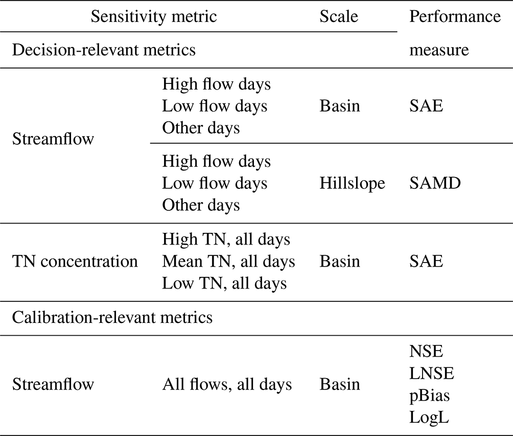
2.2.1 Decision-relevant sensitivity metrics

For the basin outlet, we used the sum of absolute error (SAE) as the performance measure for decision-relevant sensitivity metrics. For hillslopes (where observations are not available) we used the sum of absolute median deviation (SAMD), where the median value for each hillslope was computed across all model simulations. For completeness, we compared the results of using SAMD for the basin outlet to the SAE results in the Supplement (item S9). We found similar parameter selection and sensitivity ranking results for each performance measure, which demonstrates that an observation time series is not necessary to obtain the parameter set to calibrate, although observations help to check that SA model simulations are reasonable. The SAE and SAMD expressions are shown in Eqs. (1) and (2):

$$\begin{array}{}\text{(1)}& {\displaystyle }\text{Basin:}\mathrm{SAE}=\sum _{t=\mathrm{1}}^T\left|{\mathit{Q}}_{\mathrm{sim}}\left[t\right]-{\mathit{Q}}_{\mathrm{obs}}\left[t\right]\right|\text{(2)}& {\displaystyle }\text{Hillslope:}\mathrm{SAMD}=\sum _{t=\mathrm{1}}^T\left|{\mathit{Q}}_{\mathrm{sim}}\left[t\right]-\mathrm{med}\left({\mathbf{Q}}_{\mathrm{sim}}\right[:,t\left]\right)\right|,\end{array}$$

where T is the total number of time series data points for the sensitivity metric, Q_sim is the time series of the simulated quantity (e.g., streamflow), Q_obs is the vector of the observed quantity, and $\mathrm{med}\left({\mathbf{Q}}_{\mathrm{sim}}\right[:,t\left]\right)$ is the median simulated quantity at time t over all of the model runs completed for sensitivity analysis, as stored in matrix Q_sim.

We consider sensitivity metrics that are relevant to water quantity and quality outcomes because they are among the most common for hydrological modeling studies. For water quantity, we compute SAE (basin) and SAMD (hillslopes) for three mutually exclusive flows: (1) high flows greater than the historical 95th percentile, (2) low flows less than the historical 5th percentile, and (3) all other flows between the historical 5th and 95th percentiles. The SAE and SAMD are computed for the T days on which these flows occurred. The percentiles are estimated based on the calibration data (described in Sect. 4). Variability in the resulting sensitivity metrics and screened parameters would be a function of the physical processes that generate these flows. The dates corresponding to flood flows provided a good sampling across all years of record. For low flows, most dates correspond to a drought in 2007. Therefore, using the historical 5th percentile as a metric could capture decision-relevant low flows, but could be overly sensitive to one particular period of the record. We compared results obtained from using each water year's daily flows less than that year's 5th percentile with results obtained from using the historical 5th percentile. The parameters that would be selected for calibration were identical for the example presented in this paper, so we display only the historical 5th percentile results.

For water quality, we consider the estimated daily total nitrogen (TN) concentration. As described in Sect. 3.1, we use a linear regression model with normal residuals to estimate the log-space TN concentration at the outlet as a function of time, season, and streamflow at the same location. As such, we could compute sensitivity metrics for the estimated mean and quantiles from the regression error model. The water quality sensitivity metrics are the SAE for (1) the 95th percentile of the distribution of estimated TN concentration, (2) the 5th percentile, and (3) the log-space mean (real space median) for each of the days on which TN was sampled. Therefore, unlike the streamflow metrics, these metrics are used to test if different parameters are screened for different error quantiles, and they are only applied to the basin outlet.

2.2.2 Calibration-relevant sensitivity metrics

Four performance measures that are typically used to calibrate hydrological models are used as calibration-relevant sensitivity metrics (e.g., Moriasi et al., 2007): the Nash–Sutcliffe efficiency (NSE), the NSE of log-space simulations (LNSE), the percent bias (pBias), and the log of the likelihood model that describes residual errors for streamflow (e.g., Smith et al., 2015). These metrics can only be computed for gauged locations, which is the basin outlet in this study. The first three metrics are defined in Eqs. (3)–(5):

$$\begin{array}{}\text{(3)}& {\displaystyle }\mathrm{NSE}=\mathrm{1}-{\displaystyle \frac{\sum _{t=\mathrm{1}}^T\left({\mathit{Q}}_{\mathrm{sim}}\right[t]-{\mathit{Q}}_{\mathrm{obs}}[t]{)}^{\mathrm{2}}}{\sum _{t=\mathrm{1}}^T\left({\mathit{Q}}_{\mathrm{obs}}\right[t]-\mathbb{E}[{\mathit{Q}}_{\mathrm{obs}}]{)}^{\mathrm{2}}}}\text{(4)}& {\displaystyle }\mathrm{LNSE}=\mathrm{1}-{\displaystyle \frac{\sum _{t=\mathrm{1}}^T\left(\ln \right[{\mathit{Q}}_{\mathrm{sim}}\left[t\right]]-\ln [{\mathit{Q}}_{\mathrm{obs}}\left[t\right]]{)}^{\mathrm{2}}}{\sum _{t=\mathrm{1}}^T\left(\ln \right[{\mathit{Q}}_{\mathrm{obs}}\left[t\right]]-\mathbb{E}[\ln \left({\mathit{Q}}_{\mathrm{obs}}\right)]{)}^{\mathrm{2}}}}\text{(5)}& {\displaystyle }\mathrm{pBias}=\mathrm{100}\times {\displaystyle \frac{\sum _{t=\mathrm{1}}^T\left({\mathit{Q}}_{\mathrm{sim}}\right[t]-{\mathit{Q}}_{\mathrm{obs}}[t\left]\right)}{\sum _{t=\mathrm{1}}^T{\mathit{Q}}_{\mathrm{obs}}\left[t\right]}},\end{array}$$

where ln is the natural logarithm, 𝔼 is the expectation operator, and other terms are as previously defined. The NSE is more sensitive to peak flows due to the squaring of residual errors, so it is hypothesized that parameters screened by NSE will be most similar to those screened by the high flow decision-relevant metric, although there are known issues with using NSE as a peak flow metric (e.g., Mizukami et al., 2019). The LNSE squares log-space residuals, so it assigns more equal weight to all flows; however, it is common to use LNSE to calibrate low flows. The pBias considers the scaled error, so it should assign the most equal weight to all flows.

We selected the skew exponential power (generalized normal) distribution (Schoups and Vrugt, 2010) as the likelihood model due to its ability to fit a wide variety of residual distribution shapes that could result from random sampling of hydrological model parameters. We used an implementation with two additional parameters that describe heteroskedasticity as a function of flow magnitude and a lag-1 autocorrelation, both of which are common in hydrological studies. The probability density function and resulting log likelihood (LogL) have lengthy derivations provided in Schoups and Vrugt (2010), as summarized in Appendix A with minor changes for our study. We used maximum likelihood estimation to obtain point estimates of the six likelihood model parameters, as described in the Supplement (item S0). We assume that this likelihood model would be maximized in calibration of the selected model parameters.

2.3 Morris global sensitivity analysis

Sensitivity analysis methods can be local about a single point or global to summarize the effects of parameters on model outputs across the specified parameter domain (e.g., Pianosi et al., 2016). A global method is implemented for this study because the goal is to screen parameters for use in model calibration. The Method of Morris (1991) derivative-based sensitivity analysis is employed as a computationally fast method whose parameter rankings have been shown to be similar to more expensive variance-based analyses (Saltelli et al., 2010) for spatially distributed environmental models (Herman et al., 2013a).

The Method of Morris is based on elementary effects (EEs) that approximate the first derivative of the sensitivity metric with respect to a change in a parameter value. The EEs are computed by changing one parameter at a time along a trajectory, and comparing the change in sensitivity metric from one step in the trajectory to the next. The change is normalized by the relative change in the parameter value (Eq. 7). Assuming that the pth parameter is changed on the (s+1)th step in the jth trajectory, the EE for parameter p using the computed sensitivity metrics (SMs) (SAE, NSE, etc.) is computed as shown in Eq. (6):

$$\begin{array}{}\text{(6)}& {\displaystyle }\mathbf{EE}[j,p]={\displaystyle \frac{\mathbf{SM}[j,s+\mathrm{1}]-\mathbf{SM}[j,s]}{{\mathrm{\Delta }}_{\mathrm{s}+\mathrm{1},\mathrm{s},\mathrm{p}}}}\text{(7)}& {\displaystyle }{\mathrm{\Delta }}_{\mathrm{s}+\mathrm{1},\mathrm{s},\mathrm{p}}={\displaystyle \frac{\mathbf{X}[j,s+\mathrm{1},p]-\mathbf{X}[j,s,p]}{\left|\max \right(\mathbf{X}[:,:,p])-\min (\mathbf{X}[:,:,p]\left)\right|}},\end{array}$$

where EE is the elementary effect matrix consisting of one row per trajectory and one column per parameter, ${\mathrm{\Delta }}_{\mathrm{s}+\mathrm{1},\mathrm{s},\mathrm{p}}$ is the change in the value of the parameter as a fraction of the selected parameter range, and X is the matrix of parameter values. The EEs for each parameter are typically computed in tens to hundreds of locations in the parameter domain, and are then summarized to evaluate global parameter importance. The mean absolute value of the EEs computed over all of the r locations (one for each trajectory) is the summary statistic used to rank model sensitivity to each parameter, as recommended by Campolongo et al. (2007). The sample estimator is provided in Eq. (8):

$$\begin{array}{}\text{(8)}& {\widehat{\mathit{\mu }}}_{\mathrm{p}}^{*}={\displaystyle \frac{\mathrm{1}}{r}}\sum _{j=\mathrm{1}}^r\left|\mathbf{EE}\right[j,p\left]\right|.\end{array}$$

We used 40 trajectories that were initialized by a Latin hypercube sample, and used the R sensitivity package (Iooss et al., 2019) to generate sample points and compute EEs. Each parameter had 100 possible levels that were uniformly spaced across its specified range. Step changes, Δ, in parameter values were set to 50 levels (i.e., 50 % of their range). For each parameter, this allows for a uniform distribution of parameter values across all samples (example sampling distributions for other percentages are provided in Supplement item S8). We adjusted some trajectory sampling points to satisfy inequality and simplex constraints within the RHESSys model (described in Supplement item S0).

2.4 Parameter selection based on bootstrapped error

After the hydrological model runs completed for all trajectories, we estimated 90 % confidence intervals for each parameter's ${\widehat{\mathit{\mu }}}_{\mathrm{p}}^{*}$ by bootstrapping. For each parameter, 1000 EE vectors of length r had their elements sampled with replacement from the original r EEs, and ${\widehat{\mathit{\mu }}}_{\mathrm{p}}^{*}$ was computed for each vector. We independently completed bootstrapping for each parameter (as in the SALib implementation by Herman and Usher, 2017) instead of sampling whole Morris trajectories (as in the STAR-VARS implementation by Razavi and Gupta, 2016) to allow greater variation in the resulting quantile estimates.

We used an EE cutoff to determine which parameters would be selected for calibration. For each sensitivity metric, we determined the bootstrapped mean EE value (Eq. 8) corresponding to the top Xth percentile, after removing parameters whose EEs were equal to zero. All of the parameters whose estimated 95th percentile EE values were greater than this cutoff value would be selected for calibration for that metric. The union of parameters selected from all sensitivity metrics comprised the final set of calibration parameters. We evaluated the number of parameters selected as a function of the Xth percentile cutoff for basin and hillslope outlet sensitivity analyses in Sect. 5. Subsequent results are presented for the 10th percentile as an example cutoff; in practice, the cutoff value should be defined separately for each sensitivity metric based on a meaningful change for the decision maker (e.g., the ϵ-tolerance in optimization problems; Laumanns et al., 2002). To test the hypothesis of spatial variability in parameters that affect the sensitivity metrics, we compare parameters that would be selected based on each hillslope's EEs against each other and the basin outlet selection.

2.5 Evaluating the use of parameter multipliers

We compare the EEs for parameters that are traditionally adjusted by the same multiplier to determine if all parameter EEs are meaningfully large and not statistically significantly different from each other. This would suggest that a multiplier or another regularization method may be useful to reduce the dimensionality of the calibration problem. Parameters with large and statistically significantly different EEs are candidates for being calibrated individually, as this suggests the multiplier would not uniformly influence the model outputs across adjusted parameters. More investigation on the cause for different EEs could inform the decision to calibrate individually or use a multiplier (e.g., the difference in sensitivity could be caused by the parameters acting in vastly different proportions of the watershed area). We evaluate significance using the bootstrapped 90 % confidence intervals.

3 Hydrological model description: RHESSys

We used the Regional Hydro-Ecologic Simulation System (RHESSys) for this study (Tague and Band, 2004). RHESSys consists of coupled physically based process models of the water, carbon, and nitrogen cycles within vegetation and soil storage volumes, and it completes spatially explicit water routing. Model outputs may be provided for patches (grid cells), hillslopes, and/or the basin outlet. We used a version of RHESSys adapted for humid, urban watersheds (Lin, 2019b), including water routing for road storm drains and pipe networks, and anthropogenic sources of nitrogen. It also has modified forest ecosystem carbon and nitrogen cycles (a complete summary of modifications is provided in the README file). We used GIS2RHESSys (Lin, 2019a) to process spatial data into the modeling grid and file formats required to run RHESSys. The full computational workflow that was used for running GIS2RHESSys and RHESSys on the University of Virginia's Rivanna high performance computer is provided in the code repository (Smith, 2021a).

For this paper, we classified RHESSys model parameters as structural or non-structural. A key structural modeling decision is running the model in vegetation growth mode or in static mode, which only models seasonal vegetation cycles (e.g., leaf-on, leaf-off), and net photosynthesis and evapotranspiration, and does not provide nitrogen cycle outputs. We found that randomly sampling non-structural growth model parameters within their specified ranges commonly resulted in unstable ecosystems (e.g., very large trees or unrealistic mortality). It is beyond the scope of this paper to determine the conditions (parameter values) for which ecosystems would be stable, so we used RHESSys in static mode. We used a statistical method to estimate total nitrogen (TN) as a function of simulated streamflow, as described in Sect. 3.1. Other structural modeling decisions include using the Clapp–Hornberger equations for soil hydraulics (Clapp and Hornberger, 1978), the Dickenson method of carbon allocation (Dickinson et al., 1998), and the BiomeBGC leaf water potential curve (White et al., 2000). A full list is provided in a table in the Supplement (item S2).

We categorized non-structural parameters according to the processes they control. Table 2 displays the parameter categories, processes, number of parameters in each category, and how many parameters can be adjusted by built-in multipliers. A table in the Supplement (item S2) provides a full description of each parameter, the bounds of the uniform distribution used for sensitivity analysis sampling, and justification for the parameter bounds. Hillslope and zone parameters control processes over the entire modeling domain, while land use, vegetation, building, and soil parameters could be specified for each patch modeled in RHESSys. Patch-specific parameter values for each category would result in more parameters than the number of calibration data points, so we applied the same parameter values to each land use type (undeveloped, urban, septic), vegetation type (grass and deciduous tree), and to buildings (exurban households), and grouped soil parameters by soil texture. To reduce the number of parameters to calibrate, we did not consider specific tree species and their composition across the watershed (e.g., Lin et al., 2019); all forest cover was modeled as broadleaf deciduous trees. Given the coarse spatial resolution of grouped parameters, we did not employ spatial sensitivity analysis methods that consider auto- and cross-correlations of parameter values (Koo et al., 2020b; Lilburne and Tarantola, 2009).

Table 2 RHESSys parameter categories, the processes modeled in those categories for this study, the number of unique parameters in each category, and the number of parameters that can be adjusted by built-in RHESSys parameter multipliers.

RHESSys is typically calibrated using built-in parameter multipliers, which for this study would mean using 11 multipliers to adjust 40 of the 271 possible parameters. While we know that some of these parameters are more easily measured than others, we consider all 271 parameters in the sensitivity analysis. Some parameters are structurally dependent, so we aggregated EEs for these parameters, resulting in 237 unique EEs for each sensitivity metric. (Supplement item S0 describes the aggregation method.) We assume all parameters within an aggregated set would be calibrated, but only report them as one parameter. Previous studies that implemented sensitivity analyses of RHESSys generally adjusted a subset of the multipliers by limiting the analysis to process-specific parameters that are known or expected to affect outputs of interest (e.g., streamflow in Kim et al., 2007; nitrogen export in Lin et al., 2015 and Chen et al., 2020; carbon allocation in Garcia et al., 2016 and Reyes et al., 2017; and evapotranspiration and streamflow in Shields and Tague, 2012). Most of these studies used local one-at-a-time sensitivity analysis near a best estimate of parameter values from calibration or prior information, with some exceptions that employed global sensitivity analyses (Lin et al., 2015; Reyes et al., 2017).

To our knowledge, this paper presents the first sensitivity analysis of all non-structural RHESSys model parameters. A global sensitivity analysis approach is used to discover which parameters and processes are most important to model streamflow for this study. Consequently, part of our discussion in Sect. 6 highlights those parameters that are selected for calibration based on the sensitivity analysis, yet are not adjusted using standard RHESSys multipliers or are otherwise uncommonly calibrated. Even though the results are conditional on the specific parameter ranges (Shin et al., 2013), climatic input data and model outputs (Shields and Tague, 2012), and structural equations selected (Son et al., 2019), the resulting parameter identification should be generally useful to inform future studies that use RHESSys or other ecohydrological models.

3.1 Modeling total nitrogen with WRTDS regression

We used the Weighted Regression on Time Discharge and Season (WRTDS) method (Hirsch et al., 2010; Hirsch and De Cicco, 2015) to estimate daily TN concentration as a function of simulated streamflows. Equation (9) provides the regression model

$$\begin{array}{}\text{(9)}& \begin{array}{rl}\ln \left(C_{\mathrm{TN},t}\right)& ={\mathit{\beta }}_{\mathrm{0}}+{\mathit{\beta }}_{\mathrm{1}}\ln \left(Q_t\right)+{\mathit{\beta }}_{\mathrm{2}}t+{\mathit{\beta }}_{\mathrm{3}}\sin \left(\mathrm{2}\mathit{\pi }t\right)\\ & +{\mathit{\beta }}_{\mathrm{4}}\cos \left(\mathrm{2}\mathit{\pi }t\right)+\mathit{ϵ},\end{array}\end{array}$$

where C_TN,t is the TN concentration, β_i is the ith regression model parameter, Q_t is the streamflow (discharge), t∈ℝ is a time index in years, and ϵ is residual error. The sin and cos terms model an annual cycle. We estimated regression model parameters using the observed basin outlet streamflow and TN data. The parameter estimation procedure employs a local window approach to weight observations by their proximity in t, Q_t, and day of the year. Default values of these three WRTDS window parameters did not simulate the interquartile range of TN observations well, so we used a manual selection of WRTDS parameters to improve the model fit, as described in the Supplement (item S0). Furthermore, adding a quadratic log flow term did not result in a meaningful improvement, so we used the simpler Eq. (9) model.

In order to use WRTDS for any streamflow value within the observation time period, we created two-dimensional (t, Q_t) interpolation tables for each of the five model parameters and the residual error (provided in Supplement item S6). Simulated flows that were outside of the observed range of values were assigned the parameters for the nearest flow value in the table. Extrapolation of the concentration–flow relationship to more extreme flows than were historically observed may provide inaccurate TN estimates, which is a limitation of this statistical prediction method. We expect the error from extrapolation in this basin to be low, as N loads appear to be dominated by effluent from septic systems as evidenced by isotopic sourcing (Kaushal et al., 2011, p. 8229), and septic effluent supply should be fairly steady over time. Zero flows were assigned zero concentration. These interpolation tables apply only to the concentration–flow relationship at the basin outlet. We did not estimate TN for hillslopes due to a concern that this basin outlet relationship would overestimate TN in predominately forested hillslopes that would have different concentration–flow relationships (Duncan et al., 2015) and in this watershed do not have septic sources of TN. As a result, parameter selection for hillslopes is limited to the three streamflow sensitivity metrics.

4 Case study site description

We apply these methods to a RHESSys model of the Baisman Run watershed, which is an approximately 4 km² area that is located about 20 km north-northwest of Baltimore, Maryland, USA, and is part of the larger Chesapeake Bay watershed (Fig. 1a inset map). Baisman Run was one of the Long Term Ecological Research sites for the Baltimore Ecosystem Study (Pickett et al., 2020) and has roughly 20 years of weekly water chemistry samples and daily streamflow samples measured at the watershed outlet. The Baisman Run watershed is about 80 % forested and most trees are deciduous. Exurban development is located primarily in the headwater hillslopes 9–14 where nearly all of the impervious surfaces are located (5 % of the area). The two southwest–northeast trending linear features correspond to power lines. The remaining 15 % of the watershed corresponds to grass vegetation. Soil textures are classified as riparian or non-riparian (referred to as “other” in this study). Because there is developed land, we further divided soil textures into uncompacted or compacted for a total of four soil types (Fig. 1b). The hypothetical motivation for this sensitivity analysis is to inform the selection of parameters to calibrate a RHESSys model that could be used to optimize the siting and sizing of stormwater infrastructure for flood control and nutrient reduction. After a 5-year spin-up period, we completed sensitivity analysis for 1 October 2004 to 30 September 2010. The sensitivity analysis would screen parameters for calibration and validation using the additional years of data. There was a drought and several large precipitation events in this time period that seemed representative of the remaining calibration dataset. The average annual precipitation total is about 1 m and the average monthly temperature ranges from −2 to 25 ^∘C. We provide references to code and data used for this study as well as data processing notes in the Supplement (item S0).

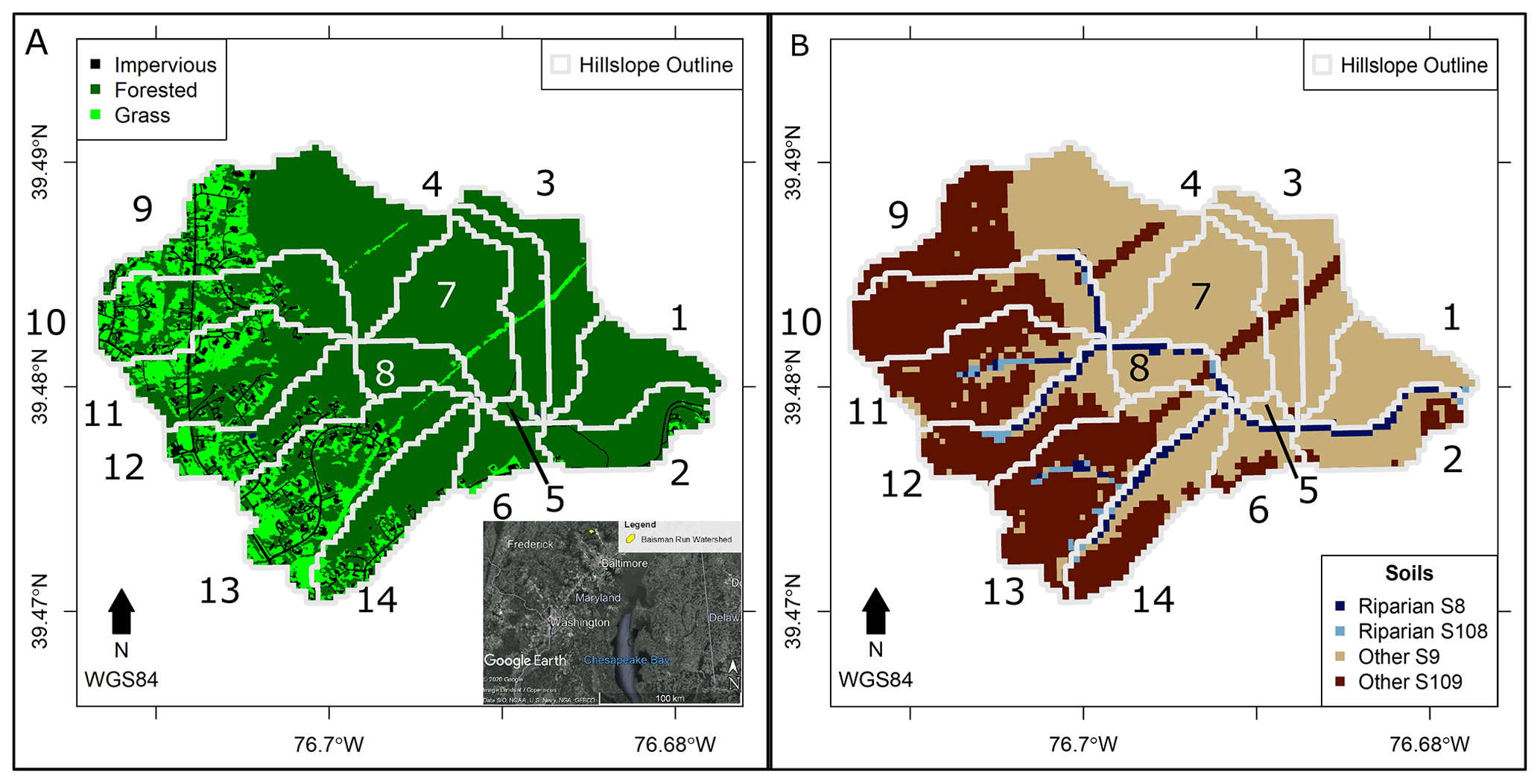
Figure 1 (a) Land cover of the Baisman Run watershed (data provided by Chesapeake Conservancy, 2014), and an inset map showing the location in the USA (Google Earth, 2020). Numbered hillslopes are outlined in gray. (b) Soil types of Baisman Run (data provided by United States Department of Agriculture (USDA), 2017). Compacted soils begin with S10.

5 Results

In Sect. 5.1 we present results for the six decision-relevant sensitivity metrics. In Sect. 5.1.1 we use these results to evaluate the appropriateness of using multipliers for calibration. Finally, we compare results for calibration-relevant and decision-relevant metrics in Sect. 5.2.

5.1 Analysis for decision-relevant sensitivity metrics

We first compare the number of parameters selected for calibration based upon decision-relevant elementary effects (EEs) whose mean or 95th percentile estimates are larger than the Xth percentile cutoff. Figure 2 shows the total number of unique parameters (out of 102 with non-zero EEs) that would be selected for calibration as a function of the cutoff value. The plotted total is the union of the top X percent across the six decision-relevant metrics for the basin outlet, and across the three streamflow metrics for hillslope outlets, so more than X percent may be selected at each cutoff value. For hillslope outlets, the union is also computed over all hillslopes. The gap in number of parameters selected when using hillslope outlets instead of the basin outlet suggests that parameters that control physical processes captured by the streamflow sensitivity metrics are different across the watershed, as explored further in Fig. 4. For this problem, considering sensitivity metrics for hillslope outlets commonly results in an additional 10–20 parameters selected for calibration compared with only using the basin outlet. There can be as many as 40 more parameters near the X=50 % cutoff. For basin and hillslope outlets, the gap between using the bootstrapped 95th percentile EE values instead of the mean values illustrates the importance of considering sampling uncertainty in parameter screening exercises. For this problem, sampling uncertainty commonly adds 5–15 additional parameters. Near the X=50 % cutoff, almost all parameters would be selected for calibration using the hillslope outlets and 95th percentile EE values. If desired, these sampling uncertainty gaps can be reduced by evaluating more Morris trajectories (e.g., by using progressive Latin hypercube sampling to add new trajectory starting points, as in Sheikholeslami and Razavi, 2017). This should bring the mean and 95th percentile lines closer together in this figure.

Figure 2 The number of parameters that would be selected for model calibration using the decision-relevant sensitivity metrics as a function of the cutoff percentage used to select parameters based on their elementary effects. The blue lines with circle points indicate the parameters that would be selected using only the basin outlet, while the gray lines correspond to using all hillslope outlets. Only streamflow metrics are considered for the hillslope outlets. Lighter line colors correspond to the bootstrapped mean and darker colors correspond to using the bootstrapped 95th percentiles of the elementary effects to select parameters. The vertical dashed line indicates the selected 10 % cutoff used as an example in this paper.

For the selected 10 % cutoff in Fig. 2, 21 unique parameters would be selected for the basin outlet using the 95th percentile EE values. Of these parameters, 18 are selected based on the three streamflow metrics and 19 are selected based on the three TN metrics. This finding supports using sensitivity metrics for each of a decision maker's objectives to inform which parameters to calibrate.

Basin outlet EEs are displayed in Fig. 3 by parameter category (color) and type within each category (shape). Of the 237 parameters, 135 had EE values of exactly 0 for all metrics (i.e., these parameters do not affect model-predicted streamflow). These parameters primarily affect the RHESSys nitrogen cycle and vegetation growth (which are not used in static mode), buildings, and some snow parameters. For streamflow sensitivity metrics (left column), differences in the selected parameters and their EEs across metrics suggest that flows of different magnitudes are affected by different physical processes, as expected (e.g., Ranatunga et al., 2016). For example, hillslope groundwater controls (index 1) and saturation to groundwater controls for compacted other soil (index 93) that affect how water moves from groundwater to riparian areas are selected parameters for each metric, but their EEs for low flows are larger than for the other metrics. This is likely because groundwater would be the source of low flows. The EE magnitude for the specific rain capacity (interception storage capacity per leaf area index (LAI)) of trees (index 162) increases from flood flows to low flows. This result suggests that the impact of water intercepted by vegetation surfaces matters more for low flows, particularly in drought-stressed ecosystems, as that water alternatively reaching the ground would have a larger impact on the resulting stormflow hydrograph compared with non-drought conditions (e.g., Scaife and Band, 2017). Septic water loads (index 13), which are modeled as constant throughout the year, have a higher mean EE for flood flows than the other streamflow metrics. This could result from uncertainty in saturated soil storage volumes leading to uncertainty in flood peaks. Similarly, the EE magnitude for tree maximum stomatal conductivity (index 119) is larger for flood flows, likely because of the impact on how quickly water can be transpired by trees. Finally, the EE for wind speed is largest for flood flows, which could be explained by the impact of wind on transpiration and the resulting reduction in the recessive limb of the hydrograph (e.g., Tashie et al., 2019). Other parameters with larger EEs generally describe soil properties that are selected or are near the cutoff point for each streamflow metric. The largest of these for all metrics is the coefficient that describes bypass flow for other soils (index 73) which cover the largest area of the lower elevations in the watershed (Fig. 1b).

For the three TN metrics (Fig. 3, right column), the parameters within the top 10 largest mean EEs are the same and their order is nearly identical when considering uncertainty. The largest EEs are close in magnitude to the 5th to 95th percentile streamflow metric. These results make sense because the TN metrics are all affected by the same streamflows, and sample collection is often limited to low and moderate flow conditions (Shields et al., 2008). The reason for differences in which parameters are selected for calibration is uncertainty in the mean EE. The EE error bars tend to be larger for the upper 95th percentile TN estimate, which results in the selection of more parameters to calibrate. This result demonstrates the value of considering both model error (different TN quantile estimates) and uncertainty in sensitivity (bootstrapped EE estimates) when selecting which parameters to calibrate. More parameters are found to be potentially influential when considering these sources of uncertainty.

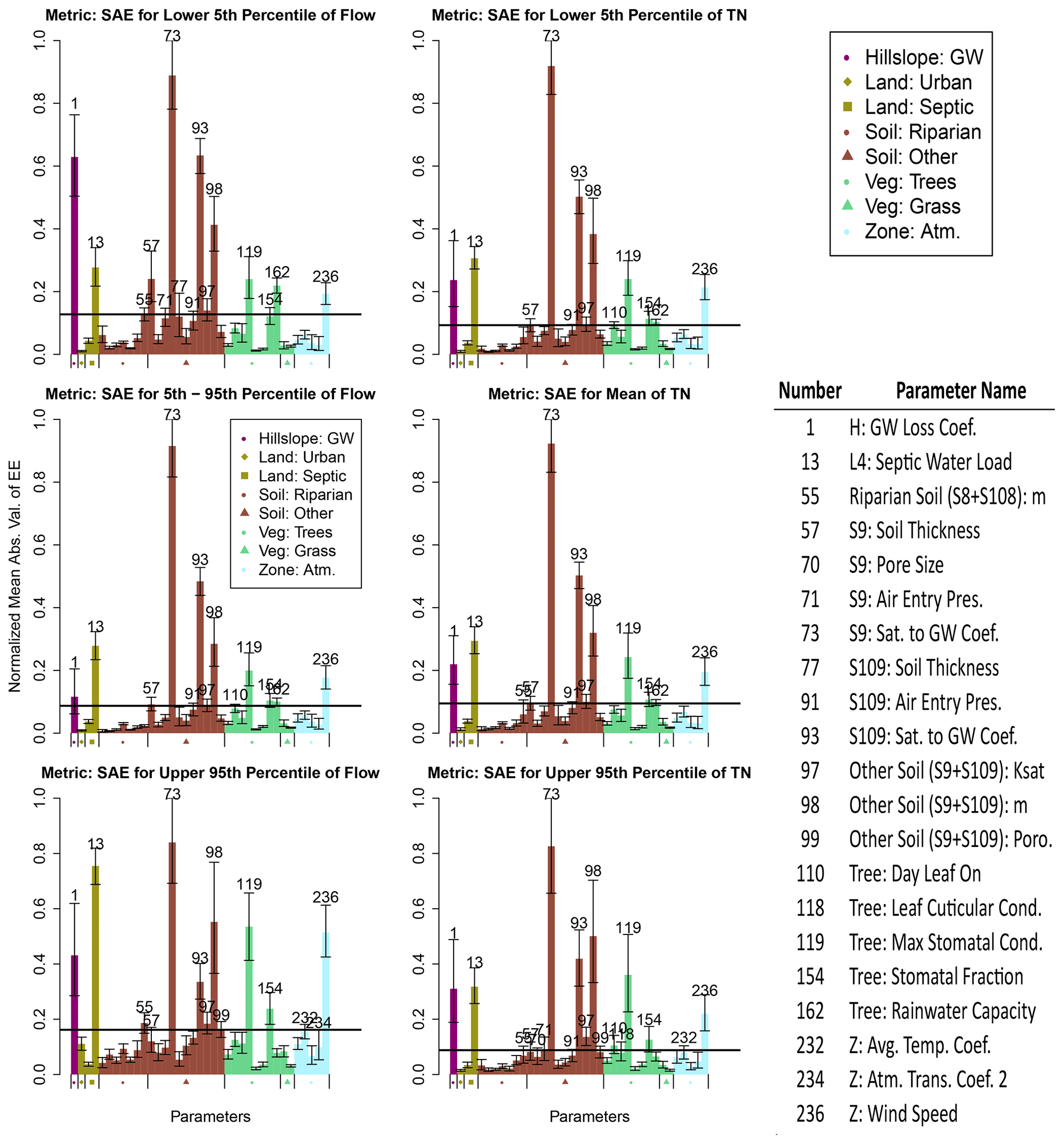
Figure 3 Mean absolute value of elementary effects for RHESSys model parameters evaluated for the six decision-relevant sensitivity metrics at the basin outlet. The EEs are normalized such that the maximum error bar value is 1 on each plot. Only parameters that would be selected by any metric presented in Table 1 are plotted in this figure. Colors indicate to which RHESSys category parameters belong, and symbols distinguish types within each category. Bootstrapped error bars extend from the 5th to 95th percentiles. Numbers above the error bars indicate the order along the x axis for parameters greater than the 10 % cutoff (horizontal black line). The numbered parameters are displayed in the accompanying table. Supplement tables contain the data plotted in this figure (item S1). GW: groundwater; K_sat: saturated hydraulic conductivity (Cond.); m: describes Cond. decay with Sat.; Poro.: porosity; Trans.: transmissivity.

For hillslope outlets, 37 unique parameters were selected using the 10 % cutoff and the 95th percentile EE values (Fig. 2). This parameter set contained all of the parameters identified using only the basin outlet. Those 37 parameters are listed in Fig. 4a and b, which compare results for each hillslope and the basin outlet. Figure 4a provides the rank of mean EEs for the upper 95th percentile streamflow sensitivity metric. We provide plots for the other two streamflow sensitivity metrics in the Supplement (item S4). Figure 4b is aggregated over all decision-relevant sensitivity metrics (and spatial areas for hillslopes) and indicates whether or not the parameter would be selected for calibration.

Figure 4 (a) Ranks of mean elementary effects for the 95th percentile streamflow sensitivity metric for the basin outlet (B on x axis) and each hillslope. Ranks are grouped by 11, which is 10 % of the number of non-zero elementary effects. (b) Indicators for whether or not a parameter would be selected for calibration, aggregated over all decision-relevant sensitivity metrics and hillslope spatial areas. In (a) and (b), white horizontal lines divide parameter categories. Categories are labeled with symbols that match those in Fig. 3. Vertical white lines divide the basin results from hillslope results, and more forested hillslopes from more impervious hillslopes. Abbreviations are the same as in Fig. 3.

Figure 4a for the flood flow sensitivity metric shows that the previously described parameters with high mean EE ranks based on the basin outlet tend to also have high mean EE ranks in all hillslopes. Septic water load and riparian soil m (hydraulic conductivity decay with saturation deficit) are exceptions, which only affect hillslopes with households and modeled riparian soils, respectively. Whether or not a hillslope is more forested or impervious explains many parameter rank differences among hillslopes (e.g., the percent impervious parameters). Tree parameters overall have higher ranks for more forested hillslopes, and grass parameters have higher ranks in more impervious hillslopes, which also have more grass areas. Compacted soils S108 and S109 have higher parameter ranks in more impervious hillslopes where these soils have larger proportions of the total hillslope area relative to more forested hillslopes. Coverage area of riparian soils is less than other soils and these soils tend to be wet regardless of the conductivity value due to spatial position, which could explain why riparian parameters tend to have smaller ranks than other soil parameters. While it is not surprising that parameter EE ranks vary across the watershed according to the hillslope features and respective processes that act in those areas (e.g., van Griensven et al., 2006; Herman et al., 2013b), this result demonstrates that evaluating sensitivity metrics across a watershed can lead to a different interpretation of which parameters are important to calibrate compared with evaluations completed for the outlet where calibration data are located.

Figure 4b further explores this point by showing which parameters would be selected for calibration using basin and hillslope analyses if aggregating the top 10 % over all decision-relevant sensitivity metrics. Comparing the parameters selected in Fig. 4b to their ranks for the flood flow sensitivity metric in Fig. 4a reveals that some lower-ranked parameters for flood flow are ultimately selected for calibration. This result supports selecting parameters based on multiple sensitivity metrics that represent all of a decision maker's objectives. Furthermore, several parameters that would be selected for hillslope analyses would not be selected for the basin analysis if sensitivity metrics were not aggregated over space, with riparian soil parameters being the most common. Three tree parameters and both grass parameters were also selected for a few hillslopes that are almost completely forested or have large grass areas, respectively, yet would not be selected for the basin analysis. Parameters that are selected for hillslopes but not for the basin would exert relatively smaller signals when calibrating to the basin outlet data, and would likely introduce equifinality to the calibration. However, there is value in considering such parametric uncertainty if the parameters have a meaningful contribution to the sensitivity of decision objectives nearer to the spatial scale of decision making (i.e., within the representative elementary watershed Reggiani et al., 1998). Specifically, engineering designs that would affect flows at these spatial scales and locations ought to be robust to the parametric uncertainty in flows that would likely result from calibration of these parameters. This point is discussed further in Sect. 6.

5.1.1 Evaluation of parameter multipliers

We present results for only those multipliers whose adjusted parameters all have non-zero EEs. Figure 5 shows barplots of the bootstrapped mean and 90 % confidence intervals of EEs for each of the 10 multiplier parameters that could be used for the selected RHESSys model structure. For EEs that were related by constraints (m and hydraulic conductivity in Fig. 5) bars are plotted for their raw and aggregated values. These barplots correspond to the 95th percentile streamflow sensitivity metric. We provide plots for the other five decision-relevant sensitivity metrics in the Supplement (item S5).

We evaluate the appropriateness of using a parameter multiplier based on the magnitudes of the EEs and their uncertainty. Parameters within the sets adjusted by m and the saturation to groundwater bypass flow coefficients (Fig. 5a and b) are candidates for being calibrated individually due to statistically significant differences in EE values, and at least one soil type with a large EE value. For specific leaf area (Fig. 5i), it would be preferable to simply calibrate the tree parameter instead of using a multiplier. For the maximum snow energy deficit (Fig. 5h), using one multiplier for riparian soils and another multiplier for other soils may be preferable. For all other parameters, a single multiplier or other regularization method could be used based on overlapping error bars and/or relatively small EE values. These results hold well across the six decision-relevant sensitivity metrics and suggest that the dimensionality of the calibration could be reduced by employing parameter multipliers or another regularization method (e.g., Pokhrel and Gupta, 2010). Specifically for multipliers, if all 38 unaggregated parameters in this figure were selected for calibration, the aforementioned suggested multipliers could reduce the calibrated total to 15. Depending on the EE percentile cutoff used to select parameters (Fig. 2), the bottom row and possibly the middle row in Fig. 5 may not be selected for calibration.

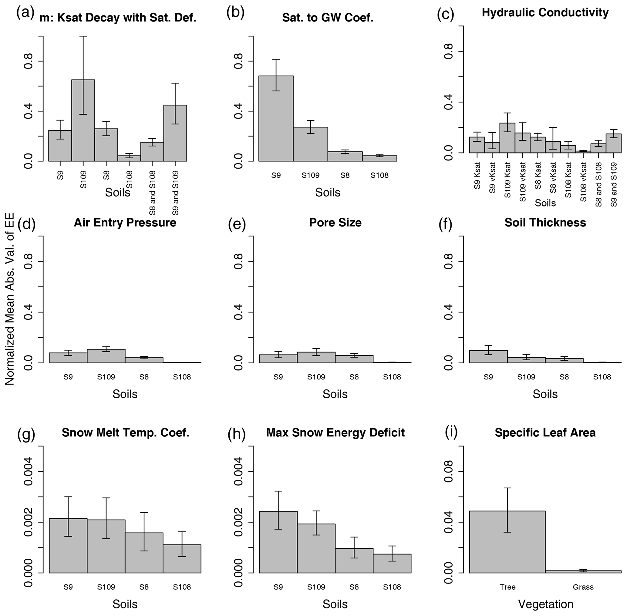
Figure 5 Barplots of the mean absolute value of the elementary effects for parameters that can be adjusted by 10 RHESSys multiplier parameters (panel (c) contains two multipliers). Bootstrapped error bars extend from the 5th to 95th percentile estimates. The effects correspond to the 95th percentile streamflow sensitivity metric and are all normalized using the same maximum error bar value as in Fig. 3. The x axis of each plot indicates which soil or vegetation type is considered. For hydraulic conductivity, it also indicates which parameter is considered (vertical (vKsat) or lateral (K_sat) conductivity). Note that the plots in the bottom row have different y axes ranges than each other and the plots above.

5.2 Analysis for calibration-relevant sensitivity metrics

Figure 6 provides plots of parameter EEs for the four calibration-relevant sensitivity metrics. The parameters with the largest EEs are nearly identical for the NSE, LNSE, and pBias metrics, and the EE magnitudes are closest to the 5th to 95th percentile streamflow metric. (These metrics are highly correlated, as shown in item S7 in the Supplement.) Contrasting these results with Fig. 3 suggests that the NSE and LNSE are not sufficient to capture parameters that affect flood and low flows, contrary to reasoning often provided as justification for their use. The log-likelihood metric shows large EEs for many of the same parameters as other calibration and decision-relevant metrics; however, the magnitudes and rankings of parameters are different, and some new parameters are selected. Note that all parameters have non-zero EEs for the LogL metric as a result of equifinality in the parameters obtained from maximum likelihood estimation. The 10 % threshold cutoff used to select parameters for calibration is larger than the resulting noise that is introduced into the EE values.

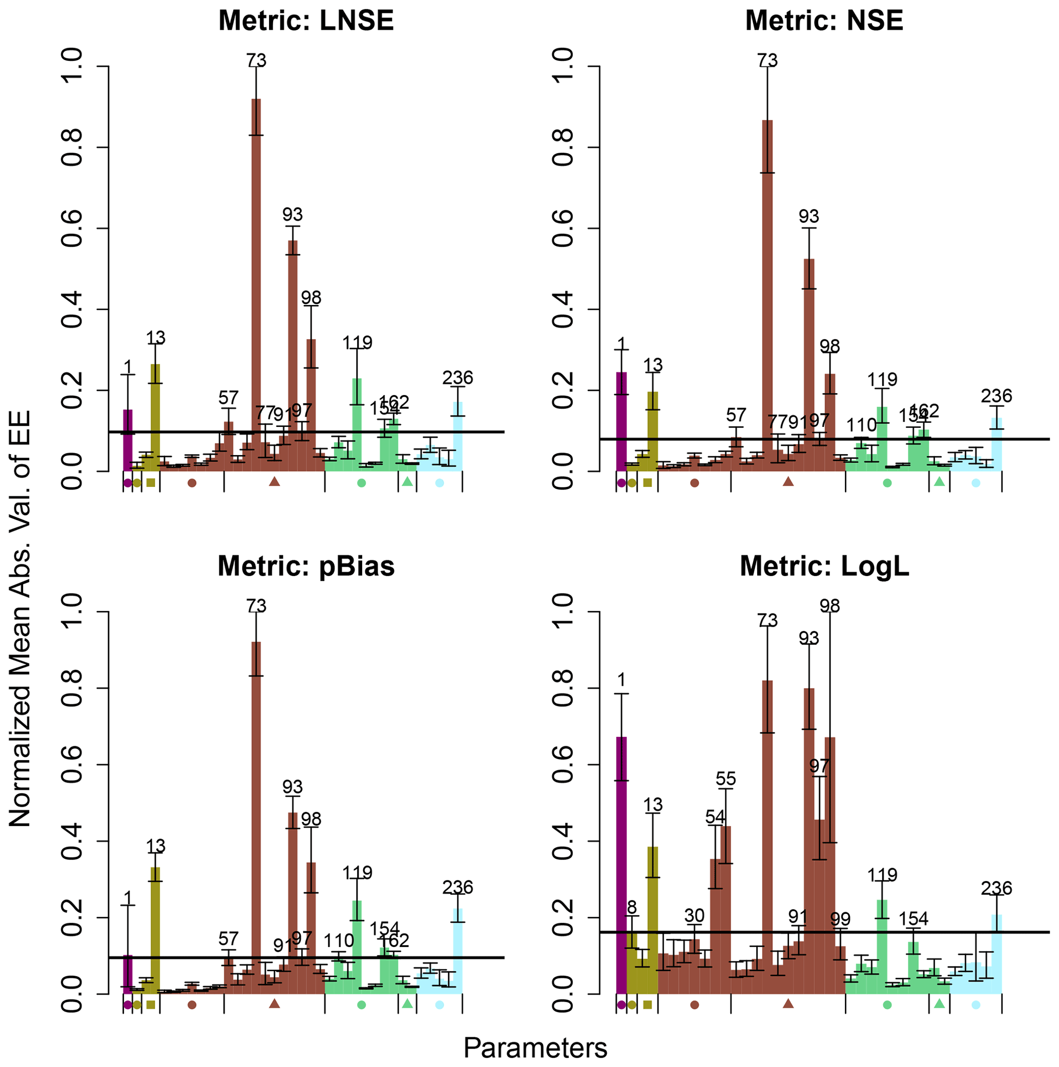
Figure 6 Mean absolute value of elementary effects for RHESSys model parameters evaluated for the four calibration-relevant sensitivity metrics at the basin outlet. The style matches Fig. 3.

Figure 7 presents a plot indicating whether or not each parameter would be selected for calibration using the calibration-relevant and decision-relevant sensitivity metrics. Note that the calibration-relevant metrics did not identify any new parameters than the decision-relevant metrics evaluated across hillslopes (All, H), so the y axis matches Fig. 4a and 4b. Considering only basin outlet evaluations (All, B), decision-relevant metrics identify five parameters that the calibration-relevant metrics do not identify. These parameters include two atmospheric parameters that were selected from the flood flow decision metric and a soil parameter that was selected from the low flow decision metric. The other two parameters were selected by considering model error in TN. Of the calibration-relevant metrics, only the log likelihood metric (LogL, B) identifies parameters that are unique from all other basin-evaluated metrics, but these parameters are selected for hillslopes using decision-relevant metrics (All, H). Of note is that a set of 10 parameters are selected for each of the calibration-relevant metrics and the aggregated decision-relevant metrics, and a set of 13 parameters are only selected from hillslope evaluation of the decision-relevant streamflow metrics. This result strengthens the recommendation to spatially evaluate sensitivity metrics to inform parameter selection of spatially distributed models.

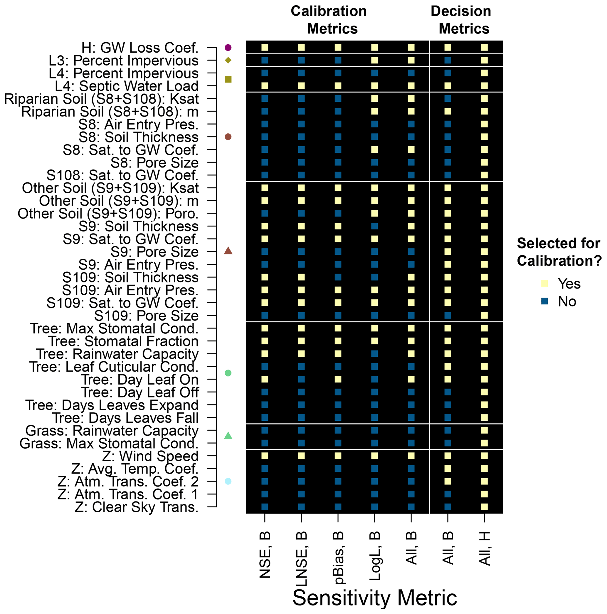
Figure 7 Indicators for whether or not a parameter would be selected for calibration for each of the calibration-relevant sensitivity metrics, and separately aggregated over all calibration-relevant and decision-relevant sensitivity metrics. B and H in the x-axis labels indicate basin outlet or hillslope outlet. Vertical white lines divide the calibration and decision-relevant sensitivity metric results. Other styles match Fig. 4b.

6 Discussion

6.1 Importance of decision-relevant sensitivity metrics for parameter screening

When sensitivity analysis is used to inform model calibrations, a primary goal is usually to reduce the dimensionality of the search space by screening those parameters that most affect the outputs to be calibrated. How model outputs are considered in sensitivity analyses and subsequent screening exercises can affect which parameters are selected. We found that specifically evaluating high and low flows as decision-relevant metrics provided a different parameter selection than using the calibration-relevant metrics that are often used to capture parameters that control such flows. While the NSE is mathematically sensitive (i.e., not robust) to high flows, the EE magnitudes and parameters that are selected by the NSE sensitivity metric do not match well with those selected from the high flows decision-relevant metric. Instead, the EE magnitudes and selected parameters resemble the 5th to 95th percentile streamflow metric. A similar result is obtained for the LNSE metric. A possible explanation for these results is that the high and low flows sensitivity metrics each represent only 5 % of the time series used in the NSE and LNSE metrics, while the 5th–95th percentile metric represents 90 % of the time series. Another possibility is that in the Baisman Run watershed, flows greater than the 95th percentile are still relatively small, and so the model residuals are a similar order of magnitude for peak flows and other flows. Regardless of the cause, this analysis demonstrates that parameter selection based on decision-relevant metrics can result in different parameters than calibration-relevant metrics. Thus, these results support future studies that would evaluate which parameter screening method is ultimately preferable for various decision problems. For example, this could be assessed by optimizing engineering designs for controlling high and low flows using models that calibrate screened parameters from the two alternative approaches.

Calibration-relevant metrics have limited value for sensitivity analyses of spatially distributed models because they can only be computed at gauged locations. The sensitivity analyses that we completed for ungauged hillslope outlets led to the identification of more parameters to calibrate than were selected based on sensitivity analysis at the gauged basin outlet. Calibrating additional parameters that have smaller impact at the gauged location is likely to exacerbate equifinality in simulated outputs. Equifinality at the basin outlet will often result in variability in outputs at ungauged locations, such that calibration of these additional parameters should be important to better capture the physical processes in hillslopes where engineering controls could be located. Even if parameter values are unchanged from their prior distributions after calibration, locations of engineering control measures can be optimized to be robust to the resulting uncertainty in model outputs across the watershed. Spatially distributed monitoring of model parameters and streamflow gauges within sub-catchments could help to reduce this uncertainty, particularly for catchments with spatially heterogeneous characteristics. In summary, spatial evaluation of sensitivity metrics for spatially distributed models allows for the discovery of parametric sources of uncertainty across the watershed to which engineering designs would have to be robust.

6.2 Determining opportunities for parameter reduction

Spatial sensitivity analyses also reveal opportunities to reduce parametric uncertainty by using additional data and data types. Parametric uncertainty could be reduced for any parameter by better constraining its prior range. For example, septic water loads could be constrained with household water consumption surveys. Surveys and data collection efforts for other parameters can target those hillslopes for which model sensitivity is largest. Alternatively, some of the parameters could instead be specified by additional input datasets to reduce the dimensionality of the calibration. For example, impervious surface percentage could be specified spatially from the land cover dataset, and time series of wind speed may be obtained from weather gauges or satellite data and then be processed to the spatial scale of the model. These approaches would transfer parametric uncertainty to input data uncertainty, which would ideally be negligible. Finally, uncertainty may be reduced by better capturing spatial trends in parameter values, for example, using finer-resolution soils data products, such as POLARIS estimates (Chaney et al., 2016), or implementing different vegetation species composition in riparian and non-riparian areas. However, both of these approaches change the RHESSys model structure and add more parameters, so it is unclear if total uncertainty would be reduced, even if local hillslope performance is improved. Nevertheless, preliminary analysis with an uncalibrated RHESSys model in dynamic mode found that simulated streamflow and nitrogen were better aligned with observations when a more spatially explicit soil and vegetation parameterization was used (Lin, 2021; vegetation by plant functional type is described in Lin et al., 2019). Similar performance was observed for soils data by Quinn et al. (2005) using RHESSys and by Anderson et al. (2006) using a SAC-SMA model. This lends support to future analyses that consider sensitivity analysis of alternative model structures and parameters to discover dominant processes, as in Mai et al. (2020) and Koo et al. (2020a). The selected parameters across water quantity and quality-focused metrics would likely be different if TN concentrations were estimated from a process-based model, as in the dynamic mode of RHESSys, instead of statistically as a function of streamflow using WRTDS (e.g., RHESSys and WRTDS estimations are compared in Son et al., 2019).

Parameter multipliers and other regularization methods are a common dimensionality reduction choice for spatially distributed models. A comparison of model sensitivity results for parameters that can be adjusted by built-in RHESSys multipliers revealed opportunities for dimensionality reduction by a multiplier, and also identified some parameters that may be better to calibrate individually for this problem. Future research is needed to formally test these recommendations for their impact on model calibration.

For RHESSys streamflow simulations, the global sensitivity analysis identified some parameters for calibration that are not commonly calibrated and should therefore be assigned priors that are adjusted to local site conditions. Studies of other models, such as NOAH-MP (Cuntz et al., 2016), have reached similar conclusions about the need to calibrate parameters that are commonly fixed. For example, in RHESSys, zone (atmospheric) parameters are typically assigned fixed site values, but this analysis suggests careful examination should be given to parameters that adjust the estimated average temperature based on the supplied minimum and maximum temperature time series. For vegetation species simulated in static mode, this analysis revealed that stomatal and leaf conductivity parameters, interception storage capacity parameters, and the parameter that sets the first day leaves show on deciduous trees were among the most important for modeling streamflow. For primarily forested hillslopes, parameters describing the length of time that leaves open and fall are also important. In addition to these parameters that are not adjusted by built-in RHESSys multipliers, many of the soil and groundwater parameters that are adjusted by multipliers were also identified as important to calibrate, which is common practice.

6.3 Opportunities for future research

This paper focuses on the importance of evaluating sensitivity analyses at the spatial scale and magnitude that is appropriate for decision making. Selecting the appropriate temporal resolution for the sensitivity metric and the time period of sensitivity analysis is also important to inform parameter selection. All of the sensitivity metrics in this paper are temporally aggregated measures instead of time-varied. With this approach, two model runs could have very different simulated time series, yet could have similar metric values. Additionally, parameters that arise from different generating processes (e.g., floods from spring snowmelts vs. summer hurricanes) would not necessarily be parsed out from any one model run. For engineering problems, a magnitude-varying sensitivity analysis (Hadjimichael et al., 2020) could be useful to identify those parameters that control specific extreme events. A time-varying sensitivity analysis (Herman et al., 2013c; Meles et al., 2021) could discover more seasonally important parameters. Related to this point, this sensitivity analysis was completed for a short 6-year period. For engineering designs that will last several decades, model sensitivity to alternative climate futures would be useful to identify additional parameters to calibrate that could become important in future climates, even if they are not historically important. Considering uncertainty in these parameters for optimizations under future climatic conditions would allow engineering designs to be robust to their uncertainty. Outside of an engineering context, Hundecha et al. (2020) showed that selecting parameters that control processes within sub-catchments is important when using calibrated models for climate change forecasts.

A final consideration for risk-based decision making is the use of deterministic or stochastic watershed models. We found that sensitivity metrics for TN model residual error resulted in a different set of parameters to calibrate than using the mean of TN. This result suggests that sensitivity analysis of stochastic watershed models could lead to different parameter selection. Future work is needed to compare sensitivity analysis and resulting parameter selection for deterministic and stochastic watershed models.

7 Conclusions

This paper provides guidance on evaluating parametric model uncertainty at the spatial scales of interest for engineering decision-making problems. We used the results of a global sensitivity analysis to evaluate common methods to reduce the dimensionality of the calibration problem for spatially distributed hydrological models. We found that the sensitivity of model outputs to parameters may be relatively large at ungauged sites where engineering control measures could be located, even though the corresponding sensitivity at the gauged location is relatively small. The spatial variation in parameters with the largest sensitivity could be described well by variation in land cover and soil features, which suggests that different physical processes have important controls on model outputs across the watershed. More calibration parameters result from sensitivity analysis at local scales (i.e., ungauged hillslopes) than do from sensitivity analysis at watershed scales. While the processes affected by the additional parameters would have a relatively small effect at the outlet location, thus exacerbating the equifinality problem during calibration, they would describe important variability in model outputs at potential engineering control locations. Thus, due to equifinality, calibration methods that estimate parameter distributions are preferable to relying upon a single “best” parameter set; considering such parametric uncertainty in optimizations of engineering control measures should help to discover solutions that are robust to it. Sensitivity analysis results were also useful to inform which parameter multipliers may be useful to employ for further dimensionality reduction.

Results from this study support two critical avenues of future research that could further inform how to employ sensitivity analyses of models that are used in decision-making problems. The literature on sensitivity analysis of hydrological models almost exclusively corresponds to deterministic outputs, whereas a stochastic framework that considers model residual error should be, and often is, used to develop engineering designs. We found that considering model error resulted in selecting additional parameters to calibrate. Future research should formally compare sensitivity analysis of deterministic and stochastic watershed models that are employed for engineering decision-making problems. We also found that the parameters screened by using common extreme streamflow calibration performance measures as sensitivity metrics do not match those parameters screened by specifically evaluating extreme flows. Future work should compare results of using screened parameters from each method to calibrate a model that is used to optimize engineering controls, evaluate which method is ultimately preferable for various decision problems, and determine whether or not there is a meaningful difference in performance of the resulting controls.

Appendix A

This appendix provides the probability density function (PDF) and the log-likelihood equations for the skew exponential power distribution that we used for the LogL sensitivity metric. We made minor changes to the equations presented in Schoups and Vrugt (2010) to apply their derivations to this problem, but most equations are identical. The PDF for a standardized skew exponential power distributed variate, a_t, at time t is described in Eq. (A1):

$$\begin{array}{}\text{(A1)}& f\left(a_t\right|\mathit{\xi },\mathit{\beta })={\displaystyle \frac{\mathrm{2}{\mathit{\sigma }}_{\mathit{\xi }}{\mathit{\omega }}_{\mathit{\beta }}}{(\mathit{\xi }+{\mathit{\xi }}^{-\mathrm{1}})}}{\exp }^{-c_{\mathit{\beta }}|{a_{\mathit{\xi }}}_t{|}^{\left(\frac{\mathrm{2}}{\mathrm{1}+\mathit{\beta }}\right)}},\end{array}$$

where ξ is the skewness parameter and β is the kurtosis parameter. Terms of the standard exponential power distribution are a function of β, as described in Eqs. (A2) and (A3):

$$\begin{array}{}\text{(A2)}& {\displaystyle }{\mathit{\omega }}_{\mathit{\beta }}={\displaystyle \frac{\left(\mathrm{\Gamma }\right[\frac{\mathrm{3}}{\mathrm{2}}(\mathrm{1}+\mathit{\beta })]{)}^{\mathrm{0.5}}}{(\mathrm{1}+\mathit{\beta })\left(\mathrm{\Gamma }\right[\frac{(\mathrm{1}+\mathit{\beta })}{\mathrm{2}}]{)}^{\frac{\mathrm{3}}{\mathrm{2}}}}}\text{(A3)}& {\displaystyle }{c}_{\mathit{\beta }}={\left({\displaystyle \frac{\mathrm{\Gamma }\left[\frac{\mathrm{3}}{\mathrm{2}}\right(\mathrm{1}+\mathit{\beta }\left)\right]}{\mathrm{\Gamma }\left[\frac{\mathrm{1}}{\mathrm{2}}\right(\mathrm{1}+\mathit{\beta }\left)\right]}}\right)}^{\left(\frac{\mathrm{1}}{\mathrm{1}+\mathit{\beta }}\right)}.\end{array}$$

Introducing skew into the standard exponential power distribution involves computing the mean and standard deviation of the skew-transformed variate, which are functions of the first (M1) and second (M2) absolute moments of the original distribution. These are described in Eqs. (A4)–(A7):

$$\begin{array}{}\text{(A4)}& {\displaystyle }{\mathit{\mu }}_{\mathit{\xi }}=M_{\mathrm{1}}(\mathit{\xi }-{\mathit{\xi }}^{-\mathrm{1}})\text{(A5)}& {\displaystyle }{\mathit{\sigma }}_{\mathit{\xi }}=-\sqrt{(M_{\mathrm{2}}-{M_{\mathrm{1}}}^{\mathrm{2}})({\mathit{\xi }}^{\mathrm{2}}+{\mathit{\xi }}^{-\mathrm{2}})+\mathrm{2}{M_{\mathrm{1}}}^{\mathrm{2}}-M_{\mathrm{2}}}\text{(A6)}& {\displaystyle }{M}_{\mathrm{1}}={\displaystyle \frac{\mathrm{\Gamma }[\mathrm{1}+\mathit{\beta }]}{\left(\mathrm{\Gamma }\right[\frac{\mathrm{3}}{\mathrm{2}}(\mathrm{1}+\mathit{\beta }){]}^{\mathrm{0.5}}\left)\right(\mathrm{\Gamma }\left[\frac{\mathrm{1}}{\mathrm{2}}\right(\mathrm{1}+\mathit{\beta }\left)\right]{)}^{\mathrm{0.5}}}}.\text{(A7)}& {\displaystyle }{M}_{\mathrm{2}}=\mathrm{1}.\end{array}$$

The ${a_{\mathit{\xi }}}_t$ variable in Eq. (A1) is defined in Eq. (A8):

$$\begin{array}{}\text{(A8)}& {a_{\mathit{\xi }}}_t=({\mathit{\mu }}_{\mathit{\xi }}+{\mathit{\sigma }}_{\mathit{\xi }}{a}_t){\mathit{\xi }}^{-\mathrm{sign}({\mathit{\mu }}_{\mathit{\xi }}+{\mathit{\sigma }}_{\mathit{\xi }}{a}_t)},\end{array}$$

where a_t is defined from the streamflow residuals, ϵ_t, that are computed after applying a magnitude-varying coefficient (Eq. A9) that adjusted RHESSys simulated streamflows, as shown in Eq. (A10):

$$\begin{array}{}\text{(A9)}& {\displaystyle }{\mathit{\mu }}_t={\exp }^{{\mathit{\mu }}_h\left|Q_t\right|}\text{(A10)}& {\displaystyle }{E}_t={\mathit{\mu }}_t{Q}_t,\end{array}$$

where Q_t is the simulated streamflow at time t and E_t is the adjusted streamflow. As a result of employing the coefficient to adjust streamflows, ϵ_t is computed with respect to E_t. Our implementation modeled lag-1 autocorrelation, ϕ₁, and heteroskedasticity (Eq. A11) of ϵ_t, which leads to a_t being defined as in Eq. (A12):

$$\begin{array}{}\text{(A11)}& {\displaystyle }{\mathit{\sigma }}_t={\mathit{\sigma }}_{\mathrm{0}}+{\mathit{\sigma }}_{\mathrm{1}}\left|E_t\right|\text{(A12)}& {\displaystyle }{a}_t={\displaystyle \frac{{\mathit{ϵ}}_t-{\mathit{ϵ}}_{t-\mathrm{1}}{\mathit{\varphi }}_{\mathrm{1}}}{{\mathit{\sigma }}_t}},\end{array}$$

where σ_t is the heteroskedasticity-adjusted standard deviation. From the above equations, there are six parameters that must be estimated: β, ξ, σ₀, σ₁, ϕ₁, and μ_h. These parameters are estimated by maximizing the log-likelihood provided in Eq. (A13):

$$\begin{array}{}\text{(A13)}& \begin{array}{rl}\mathrm{LogL}& =(T-\mathrm{1})\log \left({\displaystyle \frac{\mathrm{2}{\mathit{\sigma }}_{\mathit{\xi }}{\mathit{\omega }}_{\mathit{\beta }}}{\mathit{\xi }+{\mathit{\xi }}^{-\mathrm{1}}}}\right)-c_{\mathit{\beta }}\sum _{t=\mathrm{2}}^T|{a_{\mathit{\xi }}}_t{|}^{\left(\frac{\mathrm{2}}{\mathrm{1}+\mathit{\beta }}\right)}\\ & -\sum _{t=\mathrm{2}}^T\log \left({\mathit{\sigma }}_t\right),\end{array}\end{array}$$

where T is the total number of data points in the time series. The first two terms result from Eq. (A1) and the final term results from the residual adjustment in Eq. (A12). Unlike the implementation in Schoups and Vrugt (2010), we begin at t=2 so that no assumptions need to be made about the value of the t=0 residual (which is both not simulated and unobserved). We provide code that implements the maximum likelihood estimation in the code repository (the code is based on the spotpy Python package (Houska et al., 2015)) and provide fitting details in the Supplement (item S0).