the Creative Commons Attribution 4.0 License.
the Creative Commons Attribution 4.0 License.
 | 14 Apr 2022
Exploring the possible role of satellite-based rainfall data in estimating inter- and intra-annual global rainfall erosivity
Pasquale Borrelli
Panos Panagos
Despite recent developments in modeling global soil erosion by water, to date, no substantial progress has been made towards more dynamic inter- and intra-annual assessments. In this regard, the main challenge is still represented by the limited availability of high temporal resolution rainfall data needed to estimate rainfall erosivity. As the availability of high temporal resolution rainfall data will most likely not increase in future decades since the monitoring networks have been declining since the 1980s, the suitability of alternative approaches to estimate global rainfall erosivity using satellite-based rainfall data was explored in this study. For this purpose, we used the high spatial and temporal resolution global precipitation estimates obtained with the National Oceanic and Atmospheric Administration (NOAA) Climate Data Record (CDR) Climate Prediction Center MORPHing (CMORPH) technique. Such high spatial and temporal (30 min) resolution data have not yet been used for the estimation of rainfall erosivity on a global scale. Alternatively, the erosivity density (ED) concept was also used to estimate global rainfall erosivity. The obtained global estimates of rainfall erosivity were validated against the pluviograph data included in the Global Rainfall Erosivity Database (GloREDa). Overall, results indicated that the CMORPH estimates have a marked tendency to underestimate rainfall erosivity when compared to the GloREDa estimates. The most substantial underestimations were observed in areas with the highest rainfall erosivity values. At the continental level, the best agreement between annual CMORPH and interpolated GloREDa rainfall erosivity maps was observed in Europe, while the worst agreement was detected in Africa and South America. Further analyses conducted at the monthly scale for Europe revealed seasonal misalignments, with the occurrence of underestimation of the CMORPH estimates in the summer period and overestimation in the winter period compared to GloREDa. The best agreement between the two approaches to estimate rainfall erosivity was found for fall, especially in central and eastern Europe. Conducted analysis suggested that satellite-based approaches for estimation of rainfall erosivity appear to be more suitable for low-erosivity regions, while in high-erosivity regions (> 1000–2000 MJ mm ha−1 h−1 yr−1) and seasons (> 150–250 MJ mm ha−1 h−1 month−1), the agreement with estimates obtained from pluviographs (GloREDa) is lower. Concerning the ED estimates, this second approach to estimate rainfall erosivity yielded better agreement with GloREDa estimates compared to CMORPH, which could be regarded as an expected result since this approach indirectly uses the GloREDa data. The application of a simple-linear function correction of the CMORPH data was applied to provide a better fit to GloREDa and correct systematic underestimation. This correction improved the performance of CMORPH, but in areas with the highest rainfall erosivity rates, the underestimation was still observed. A preliminary trend analysis of the CMORPH rainfall erosivity estimates was also performed for the 1998–2019 period to investigate possible changes in the rainfall erosivity at a global scale, which has not yet been conducted using high-frequency data such as CMORPH. According to this trend analysis, an increasing and statistically significant trend was more frequently observed than a decreasing trend.
- Article
(13039 KB) - Full-text XML
-
Supplement
(636 KB) - BibTeX
- EndNote


Rainfall erosivity is among the main drivers of soil erosion, which can be characterized by large spatial and temporal variability (Angulo-Martínez and Beguería, 2012; Ballabio et al., 2017; Bezak et al., 2021; Cui et al., 2020; Panagos et al., 2017; Verstraeten et al., 2006). In order to obtain robust rainfall erosivity estimates, high temporal resolution rainfall data are needed (Panagos et al., 2015; Yin et al., 2017). However, according to Panagos et al. (2017), the availability of stations with high-frequency data that can be used to estimate rainfall erosivity is on average relatively low in many parts of the world. Therefore, in areas with scarce data availability, remotely measured precipitation data can be instrumental in estimating rainfall erosivity (Ganasri and Ramesh, 2016; Li et al., 2020). Alternatively, approaches using simpler and less data-demanding methods such as erosivity density (ED) (Nearing et al., 2017; Panagos et al., 2015, 2016b) can also represent a viable option. Another condition that determines the accuracy of the rainfall erosivity estimates is the low availability of high temporal resolution rainfall data. Ideally, high-frequency (e.g., 1 min) measurements obtained using optical disdrometers are necessary to quantify the rainfall kinetic energy (Mineo et al., 2019; Nel et al., 2010; Petan et al., 2010; Sanchez-Moreno et al., 2014) of a given storm and to calculate its rainfall erosivity. However, such measuring equipment is not commonly available in regional and national measuring networks. Therefore, due to instrumental limitations, rainfall erosivity is communally estimated using hourly or sub-hourly rainfall records (generally ranging from 5 to 60 min) collected by tipping buckets or pluviographs, which do not provide information about raindrop size distribution (Panagos et al., 2016a; Petan et al., 2010; Petek et al., 2018). These kinds of data are then used together with empirically developed equations that relate rainfall kinetic power and intensity (Brown and Foster, 1987; Carollo et al., 2017; Petan et al., 2010) to obtain rainfall erosivity estimates. Alternatively, rainfall erosivity estimates can also be performed based on the rainfall volume instead of the intensity, using daily, monthly, or annual rainfall data (Renard and Freimund, 1994; Yu and Rosewell, 1996). However, it is worth mentioning that the accuracy of rainfall erosivity estimates decreases with the increase in the temporal data resolution (i.e., from 1 min to hourly, daily, monthly, or annual data). Currently, due to data scarcity, most rainfall erosivity assessments based on long-term estimates including a period of at least 10 years are limited to a few regions (Angulo-Martínez and Beguería, 2012; Nearing et al., 2015; Panagos et al., 2015, 2017), leaving large parts of the world under-researched. In this regard, a step forward is needed to enable the generation of year-by-year and sub-annual rainfall erosivity assessments for under-researched national- or larger-scale study areas.
Recent studies have already explored the possibility of estimating rainfall erosivity using satellite-based products at regional (Li et al., 2020) and national (Chen et al., 2021; Kim et al., 2020) scales, indicating their sources of uncertainties and a generally limited accuracy (Aghakouchak et al., 2012; Ghajarnia et al., 2018; Prakash, 2019; Prakash et al., 2015; Rahmawati and Lubczynski, 2018; Seo et al., 2018; Wei et al., 2018). However, to the best of the authors' knowledge, no such study has been conducted on a global scale using high temporal resolution data. A promising alternative to the often-limited rain-gauge data may be represented by satellite-based precipitation estimates, which currently have both adequate temporal and spatial resolution (Chen et al., 2021; Kim et al., 2020; Li et al., 2020; dos Santos Silva et al., 2020; Teng et al., 2017). Moreover, once further developed and fully operational, the satellite-based methods to estimate rainfall erosivity will have lower purchasing and processing costs compared to the current ones. In addition, satellite-based rainfall erosivity estimates could be especially useful in regions where rainfall erosivity estimates are currently very limited, such as some sizable sectors of Africa, Asia, and South America.
In this study, we aim to deepen the research on the use of satellite-based rainfall data in estimating rainfall erosivity by performing a first inter- and intra-annual global-scale assessment. The Global Rainfall Erosivity Database (GloREDa) data (Panagos et al., 2017) were used to evaluate both (a) the rainfall erosivity estimates obtained by satellite-based rainfall data (i.e., CMORPH) and (b) rainfall erosivity using the ED concept. Finally, a temporal trend analysis of global rainfall erosivity is presented with corrections between data based on the CMORPH and GloREDa databases.
2.1 CMORPH
The CMORPH product is a reprocessed and bias-corrected global precipitation data set covering the area between the 60∘ S and 60∘ N parallels, with a 30 min time step and a spatial resolution of 8 km × 8 km (Xie et al., 2017, 2021). The CMORPH data are developed by the National Oceanic and Atmospheric Administration (NOAA) and cover the period from 1998 onwards. This method generally uses the precipitation estimates derived from the low Earth orbit satellite-based passive microwave observations (Kim et al., 2020). Additionally, the geostationary satellite infrared imagery is used to account for possible coverage issues (Kim et al., 2020). Since CMORPH provides an estimate of the 30 min precipitation, each 30 min rainfall rate was assumed to be constant during this time interval (Kim et al., 2020; Xie et al., 2021). This data set has already been applied to several practical applications, such as validating the climate model simulations, identifying climate extremes, forcing numerical weather models, and characterizing the global precipitation (Xie et al., 2021). Additionally, details about the methodology can be found in the literature (Chen et al., 2020; Xie et al., 2017, 2021).
2.2 GloREDa database
GloREDa was created with the objective of developing the first ever global rainfall erosivity map using high temporal resolution data (Panagos et al., 2017) and moving towards a new generation of Revised Universal Soil Loss Equation (RUSLE)-based soil erosion assessments for the present (Borrelli et al., 2017) and future climate change and land use dynamics (Borrelli et al., 2020). GloREDa contains annual rainfall estimates for 3625 stations from 63 countries with temporal resolution ranging from 1 to 60 min (Panagos et al., 2017). The data sample lengths ranged from 5 to 52 years with a mean value of around 17 years, with most of the data covering the period from 2000 to 2010 (Panagos et al., 2017). The number of stations in different continents greatly varied from around 5 % (i.e., South America and Africa) to around 48 % (i.e., Europe). Based on the station data and applying the Gaussian process regression model, the global rainfall erosivity map was also prepared (Panagos et al., 2017). Therefore, in the scope of this study, both the station (i.e., point) estimated annual rainfall erosivity and a global rainfall erosivity map (Panagos et al., 2017) were used. The spatial resolution of the global rainfall erosivity map prepared by Panagos et al. (2017) is 30 arcsec (i.e., around 1 km at the Equator). The Rainfall Erosivity Database on the European Scale (REDES) is the predecessor of GloREDa as it was developed in 2015 (Panagos et al., 2015). As the REDES made the monthly erosivity values available (Ballabio et al., 2017), the monthly rainfall erosivity maps of Europe were also used here for the comparison of CMORPH to station-based rainfall erosivity. All data sets are available in the European Soil Data Centre (ESDAC) (Panagos et al., 2012).
2.3 Rainfall erosivity calculation
In order to calculate the annual and monthly rainfall erosivity for each grid cell that is covered by the CMORPH product, the time series with a 30 min time step were extracted from the original CMORPH data set (Xie et al., 2021). For each grid cell covered by CMORPH, a 30 min precipitation time series (mm h−1) was extracted for the 1998–2019 period. The erosive events were defined according to the procedure described in the RUSLE handbook (Renard et al., 1997). Thus, two events were separated in case of less than 1.27 mm of rain within 6 h. Only erosive rainfall events with more than 12.7 mm of rain in total or 6.35 mm in 15 min were considered in the calculations (Kim et al., 2020; Renard et al., 1997). In order to calculate the specific kinetic energy eB (MJ ha−1 mm−1), the Brown and Foster (1987) equation was applied since this equation was also used by Panagos et al. (2017):
where I is rainfall intensity (mm h−1). In order to calculate the annual rainfall erosivity R factor (MJ mm ha−1 h−1 yr−1), the following two equations were also used (Renard et al., 1997):
where E is the kinetic energy of the individual erosive event (MJ ha−1), Δt is the time interval (h), and I30 is the maximum 30 min intensity (mm h−1) of erosive event n, which occurred within a time span of N years. This procedure was repeated for all grid cells covered by the CMORPH product.
2.4 ED and ERA5
The ED concept was first introduced by Kinnell (2010) and was also used in the scope of the enhanced RUSLE approach, named RUSLE2, which led to the improvements in rainfall erosivity mapping (Dabney et al., 2012; Nearing et al., 2017). The ED is defined as the ratio between annual or monthly rainfall erosivity and annual or monthly precipitation (Panagos et al., 2016b). Thus, ED is calculated as the ratio of rainfall erosivity (R) and rainfall depth (P) (Nearing et al., 2017):
Since the introduction of the ED, it has been applied in numerous studies (Diodato et al., 2019; Kinnell, 2019; Nearing et al., 2017; Panagos et al., 2016b). The global rainfall erosivity map obtained by Panagos et al. (2017) was used in this study to obtain a global rainfall ED map. For the calculation of rainfall volume for specific years, the ERA5 reanalysis product was used.
ERA5 is one of the latest reanalysis products produced by the European Centre for Medium-Range Weather Forecasts (ECMWF) that provide atmospheric, land-surface, and sea-state data. ERA5 includes a large number of historical observations and provides a long-term solution for ED estimation. The reanalysis data combine the model data and observations across the globe into a complete and consistent data set based on the laws of physics (ERA5, 2021a). Therefore, the ERA5 product is widely used for different purposes (Reder and Rianna, 2021; Sutanto et al., 2020; Tang et al., 2020). The monthly temporal resolution on a single level was used and a horizontal resolution of . The temporal coverage used in this study was from 1979 until 2020. Comparison with CMORPH and GloREDa was made using the 1998–2019 period. Additional information can be found in the existing literature (An et al., 2020; ERA5, 2021b; Tang et al., 2020). ERA5 is updated regularly (i.e., monthly updates), which makes it the best option for the dynamic rainfall erosivity assessment at a global scale using the ED concept. In the case of the ED concept, the annual and monthly ED maps (Ballabio et al., 2017; Panagos et al., 2017) were multiplied by mean monthly or annual precipitation estimates provided by ERA5.
2.5 Data evaluation
The performance of the rainfall erosivity derived using the CMORPH product and ED concept was evaluated using the GloREDa point data set (Panagos et al., 2017). This evaluation was performed for the period 1998–2019 at global, continental, catchment, and local scales. For the latter, point data values (stations) were compared against values derived at this location from both methodologies. At the catchment scale, the HydroSHEDS catchment boundaries at the third level were used (Lehner and Grill, 2013). The idea of using third-level catchment boundaries was to evaluate whether the accuracy of the CMORPH- and ED-derived rainfall erosivity changes with scale (i.e., from global to large regional or even point scale). Moreover, a more detailed comparison was made for Europe since monthly rainfall erosivity maps (REDES) are also available (Ballabio et al., 2017) and were also used for the comparison.
In the data evaluation process, we used the following metrics: Pearson correlation coefficient, percent bias, and Gini coefficient. The Pearson correlation coefficient is a measure of linear correlation between two data sets. The percent bias is a measure of the mean tendency of the modeled data to be smaller or larger than the observed data. The Gini coefficient is a scalar metric that can be derived based on the Lorenz curve and is frequently used in economics to describe the inequality of wealth (Gini, 1914; Lorenz, 1905; Masaki et al., 2014). The Gini coefficient ranges from 0 to 1, where a value close to 1 and 0 indicates significant inequality and no inequality, respectively (Masaki et al., 2014). Thus, the idea behind using the Gini coefficient was to use an additional metric that describes the distribution of rainfall erosivity in the selected area (e.g., the distribution of rainfall erosivity grid cells at catchment or continental scale). Therefore, the Gini coefficient can be used as an indicator of the rainfall erosivity spatial patterns. Figure 1 shows an example of different Gini coefficient values for three examples. In the first one, there are similar grid values, and the Gini coefficient is close to 0. The third example shows significant inequality where the Gini coefficient is close to 1, and the second example represents more diverse grid values with a Gini coefficient of around 0.5 (Fig. 1).
Since the spatial resolutions of the input data sets (CMORPH, GloREDa, and REDES) were not the same, the GloREDa and REDES data (and the ED) were resampled to the same grid system extent and resolution that were used by CMORPH using the mean value (cell-area-weighted) method that is included in the SAGA GIS software (SAGA GIS, 2021). The same applied to the ERA5 product that was also resampled to the same grid system using B-spline interpolation (SAGA GIS, 2021). Therefore, the above-described comparison at global, continental, regional, and point scales was made using the resampled GloREDa and REDES maps (Panagos et al., 2017). A preliminary investigation was done to estimate the resampling effect on the mean global rainfall erosivity. The global mean rainfall erosivity using the GloREDa map (1 km spatial resolution) was 2190 MJ mm ha−1 h−1 yr−1, while in the case of resampled (i.e., mean) data at 10 km resolution, this value is equal to 2260 MJ mm ha−1 h−1 yr−1. Thus, resampling led to an around 3 % difference in the global mean value. However, further aggregation of the GloREDa data led to larger differences.
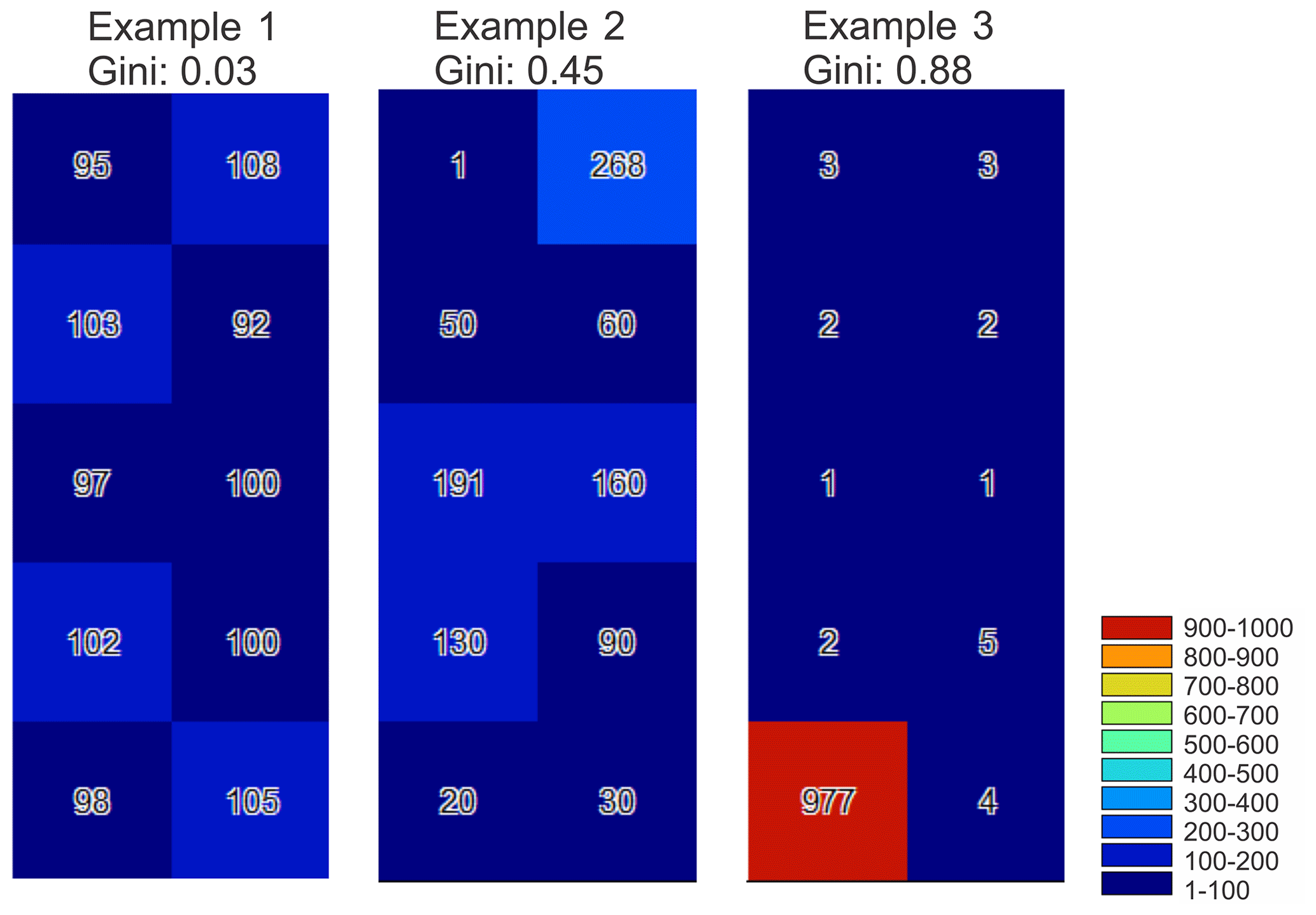
Figure 1Gini coefficients for three examples of 10 grid cells with the same mean value (i.e., 100) as an illustration of the added value of the Gini coefficient. Example 1 has similar grid values (i.e., low Gini value), example 2 has more diverse grid values (i.e., Gini value around 0.5), and example 3 has significant inequality (i.e., Gini value close to 1).
2.6 Trends
Based on the annual CMORPH and ED global rainfall erosivity maps for specific years in the period from 1998 to 2019, the Mann–Kendall trend test was also calculated for each grid cell. The Mann–Kendall test is one of the most widely applied tests for the detection of changes in the environmental data (Burn and Hag Elnur, 2002; Rodrigues da Silva et al., 2016). A detailed description of the Mann–Kendall test can be found in the literature (Burn and Hag Elnur, 2002; Hamed, 2008; McLeod, 2011). The objective was to identify areas where the detected trend in the annual rainfall erosivity data was positive or negative with a significance level of 0.05.
3.1 Spatial distribution of annual rainfall erosivity
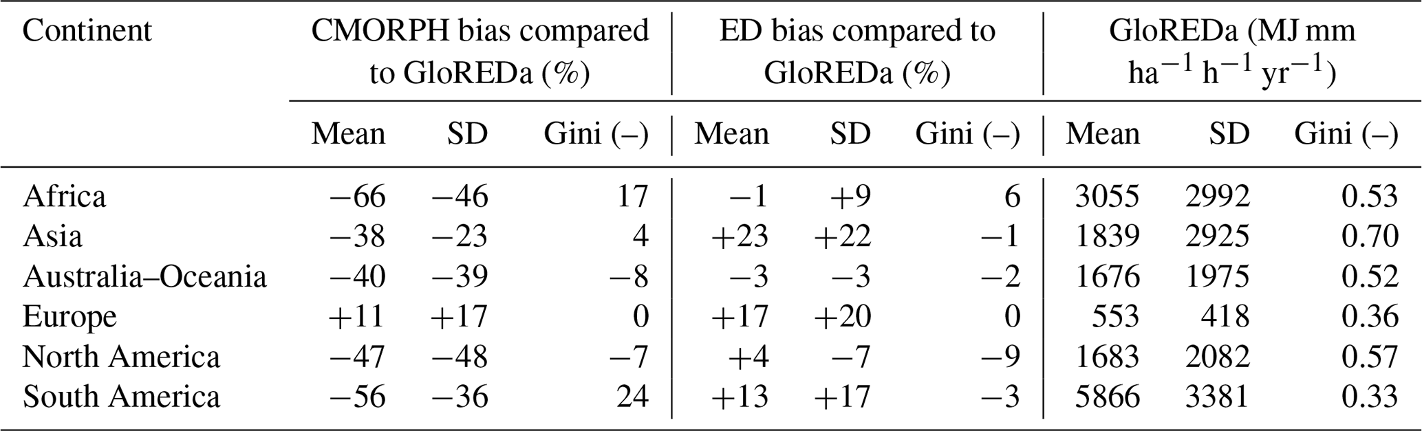
The mean global annual rainfall erosivity using the CMORPH (Fig. 2a) data is 1236 MJ mm ha−1 h−1 yr−1, with a standard deviation of 1895 MJ mm ha−1 h−1 yr−1. The mean global annual rainfall erosivity using the ED approach (Fig. 2b) is 2480 MJ mm ha−1 h−1 yr−1. As can be inferred from Fig. 2 and as further indicated in Table 1, CMORPH and ED approaches both agreed that the highest values of rainfall erosivity at the continental level were estimated for South America, while the smallest ones were estimated for Europe.
Concerning the inequality of CMORPH estimates, the Gini coefficient reflects a high level of rainfall erosivity inequality for Asia, followed by Africa and North America, while the smallest value was observed for Europe (Table 1). Also, with regard to the ED concept, the largest Gini coefficient was obtained for Asia, whereas Europe has the smallest value (Table 1). Both the mean global rainfall erosivity map for the 1998–2019 period based on the CMORPH product (Fig. 2a) and the one developed by using the ED concept and ERA5 will be available in ESDAC (Panagos et al., 2012).
Table 1Mean, standard deviation, and Gini coefficient of the global rainfall erosivity maps derived using CMORPH and ED.
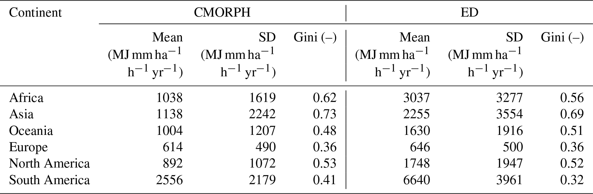
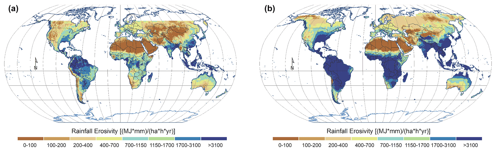
Figure 2Mean global rainfall erosivity map for the 1998–2019 period based on the CMORPH product (a) and ED concept using ERA5 (b).
3.2 Temporal trends in rainfall erosivity
Table 2 shows the mean and standard deviation of monthly rainfall erosivity derived using the CMORPH product. One can notice that the highest rainfall erosivity values were obtained in July, followed by August, and the lowest were in November (Table 2).
The temporal trends for both CMORPH- and ED-derived rainfall erosivity data sets were also calculated. The annual rainfall erosivity in the period 1998–2019 ranged from 990 to 1440 MJ mm ha−1 h−1 yr−1 using the CMORPH data (Figs. 3, S1). Using the ED concept for global rainfall erosivity assessment, the mean value ranged from 2380 to 2602 MJ mm ha−1 h−1 yr−1 (Figs. 3, S1) for the period 1998–2019. In addition, the fluctuation of the mean annual erosivity in relation to the ED concept was smaller compared to CMORPH (Fig. 3), a condition which can be related to the fact that the adopted ED concept used a constant ED map for the entire period, while only annual precipitation (i.e., ERA5) changed from year to year.

Figure 3Trend analysis for the mean and standard deviation (SD) for annual rainfall erosivity (R) using CMORPH and ED.
3.3 Data evaluation
3.3.1 Comparison at a global scale
For most continents, relatively large differences in the mean long-term annual rainfall erosivity between GloREDa and CMORPH were observed, while smaller differences were observed between ED and GloREDa, which could be expected due to the selected ED input data (Table 3). The most significant differences in the case of CMORPH were detected for Africa, South America, and North America (Table 3). As for the ED concept, the most considerable differences were calculated for Asia, Europe, and South America. On the other hand, much better agreement between the CMORPH and GloREDa maps was observed for Europe and partly for Asia (Table 3). In terms of the Gini coefficient, smaller bias values were obtained compared to the mean annual rainfall erosivity (Table 3). Thus, it seems that the distribution of the rainfall erosivity of CMORPH, ED concept, and GloREDa was relatively similar (i.e., smaller bias) despite the fact that the GloREDa map was based on interpolation. It should be noted that the ED provided a better fit to GloREDa compared to CMORPH at most of the continents in terms of the Gini coefficient, which means that the spatial rainfall erosivity patterns are quite similar. This can be regarded as an expected result since the ED indirectly uses the GloREDa data.
Table 2Global monthly rainfall erosivity values using the CMORPH product. Mean and standard deviation are shown.
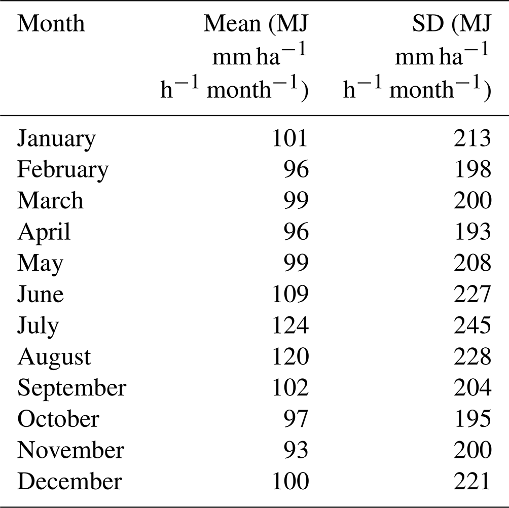
Table 3A comparison between CMORPH-, ED-concept-, and GloREDa-derived global rainfall erosivity at a continental scale.
3.3.2 Comparison at regional scale
The HydroSHEDS catchment boundaries (Lehner and Grill, 2013) at the third level were used to compare the data of CMORPH to GloREDa at the regional scale. Thus, the global land surface was divided into 288 sub-catchments at the third level with a mean catchment area of around 460 000 km2. Hence, this can be regarded as an extensive regional-scale investigation. The results demonstrated that the Pearson correlation between the mean annual rainfall erosivity at the sub-catchment level (sub-catchment average values were used) between CMORPH and GloREDa was 0.81 (R2=0.66 with p value <0.01). Moreover, the mean bias was around −50 % in case GloREDa data were considered to be the observed data. In terms of the Gini coefficient, the Pearson correlation coefficient was 0.56 (R2=0.31 with p value <0.01), while the mean bias was equal to 45 %. Therefore, CMORPH yielded more unequal (i.e., larger Gini coefficient) spatial erosivity patterns compared to GloREDa, which was based on interpolation. The spatial interpolations tend to smooth the extreme values (Dodson and Marks, 1997); therefore, Gini is smaller.
The comparison between the ED concept and GloREDa revealed that the Pearson correlation coefficient was equal to 0.95 (R2=0.90 with p value <0.01), and the mean bias was 7 %. Regarding the Gini coefficient, the Pearson correlation coefficient and the mean percent bias were 0.91 (R2=0.83 with p value <0.01) and 3.4 %, respectively. Therefore, GloREDa and ED maps have similar spatial erosivity patterns, which can be regarded as an expected result since the ED indirectly uses the GloREDa information. Furthermore, two examples of good (Fig. 4) and bad (Fig. 5) agreement between CMORPH, ED, and GloREDa are presented.
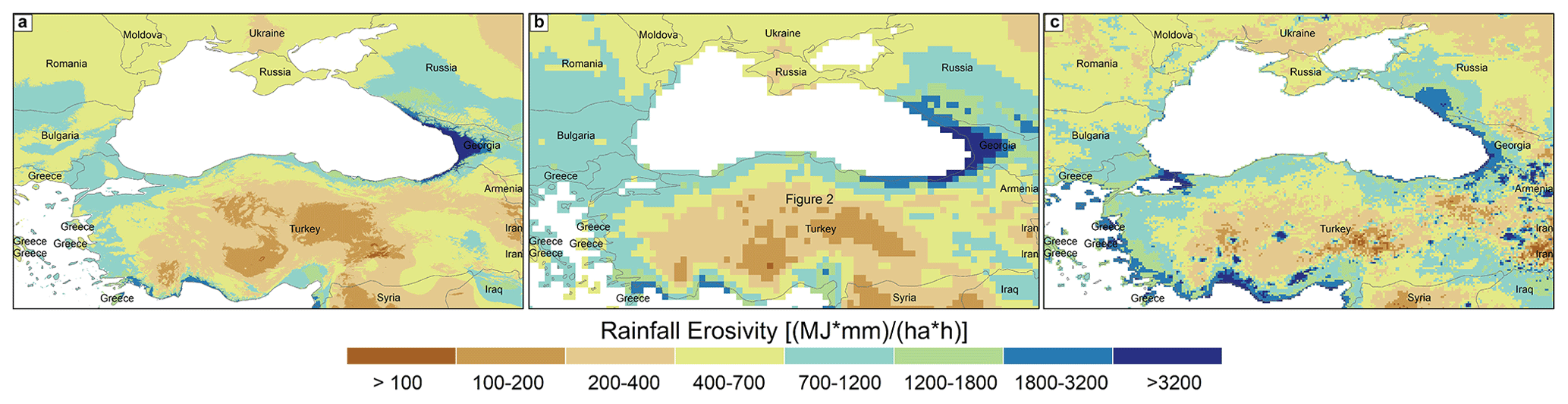
Figure 4An example of relatively good agreement between the GloREDa (a), ED (b), and CMORPH (c) maps for parts of eastern Europe and Turkey.
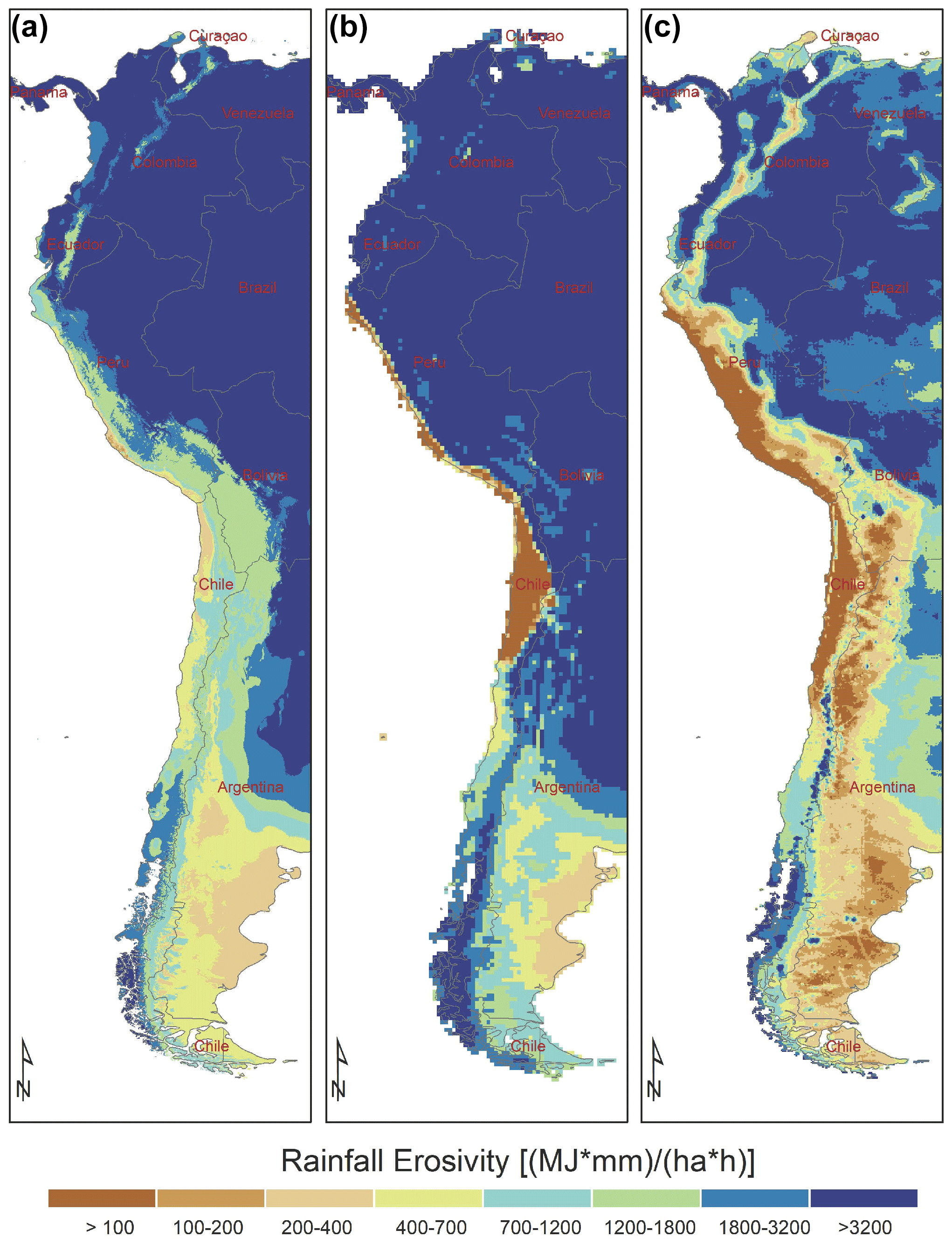
Figure 5An example of worse agreement between the GloREDa (a), ED (b), and CMORPH (c) maps for the parts of South America.
In Europe, we found the best agreement between CMORPH and GloREDa (Table 3) and the smallest uncertainty in GloREDa. For those reasons and due to the availability of monthly rainfall erosivity estimates (Ballabio et al., 2017), a more in-depth assessment was made for Europe. According to GloREDa, the mean annual rainfall erosivity in Europe (i.e., without Russia) was 668 MJ mm ha−1 h−1 yr−1 with a standard deviation of 429 MJ mm ha−1 h−1 yr−1 (Fig. 6). According to the CMORPH product, the mean and standard deviation were equal to 752 and 533 MJ mm ha−1 h−1 yr−1, respectively (Fig. 6). Additionally, the ED concept yielded a mean annual rainfall erosivity value of 804 with a standard deviation of 541 MJ mm ha−1 h−1 yr−1 (Fig. 6). Moreover, the calculated Gini coefficient using all grid cells was 0.31 in all cases (Fig. 6). Thus, it can be seen that the CMORPH product yielded a relatively similar erosivity distribution across Europe (without Russia) compared to GloREDa, which means that all maps have a similar level of inequality (i.e., non-uniform distribution of rainfall erosivity). Slightly larger rainfall erosivity values were obtained using the ED concept. It should be noted that part of these differences can be attributed to the fact that the GloREDa data set mostly used data in the 2000–2010 period (Panagos et al., 2017). Moreover, in some areas (e.g., Italy, Balkan Peninsula, parts of eastern Europe), spatial patterns in all cases were similar, although the CMORPH product and ED concept yielded slightly variable rates (Fig. 6). On the other hand, CMORPH yielded higher annual rainfall erosivity values compared to the GloREDa map in some parts of the United Kingdom and eastern Europe (Fig. 6). Furthermore, CMORPH tends to underestimate areas with relatively high rainfall erosivity such as the Alpine region, Spain, Italy, and other parts of the Mediterranean basin (Fig. 6).
As there are available monthly erosivity data sets in the EU (Ballabio et al., 2017), we compared them to the CMORPH- and ED-derived maps (Table 4). Better agreement between CMORPH and GloREDa for fall compared to winter and summer was found (Table 4). The ED concept yielded higher rainfall erosivity values in almost all months, which also resulted in higher differences at the annual level (Table 4). This could be attributed to the underestimation of the WorldClim V1 map (Beck et al., 2020). In addition, GloREDa has lower values compared to REDES in Europe.
Moreover, Fig. 7 shows monthly erosivity values for selected months where three cases were selected (i.e., underestimation, overestimation, and almost complete agreement between CMORPH and GloREDa). In July, the CMORPH product in the Alpine region generally yielded smaller erosivity values compared to both the monthly erosivity maps prepared by Ballabio et al. (2017) and the ED map (Fig. 7). The same conclusion is reached for other regions such as parts of western Europe or the Iberian Peninsula (Fig. 7). In December, parts of eastern Europe have better agreement among the three maps (Fig. 7). On the other hand, October is the month with the best agreement among the three tested maps (Fig. 7). For October, the best agreement is found in parts of eastern and central Europe, while the worst was detected in parts of the Iberian Peninsula (Fig. 7). The CMORPH-derived rainfall erosivity, in some cases, is more equally distributed (i.e., winter), and in other cases it is more unequally distributed (i.e., summer) compared to GloREDa, while in the case of the ED concept and GloREDa, the derived Gini coefficients are relatively similar throughout the year (Table 4).
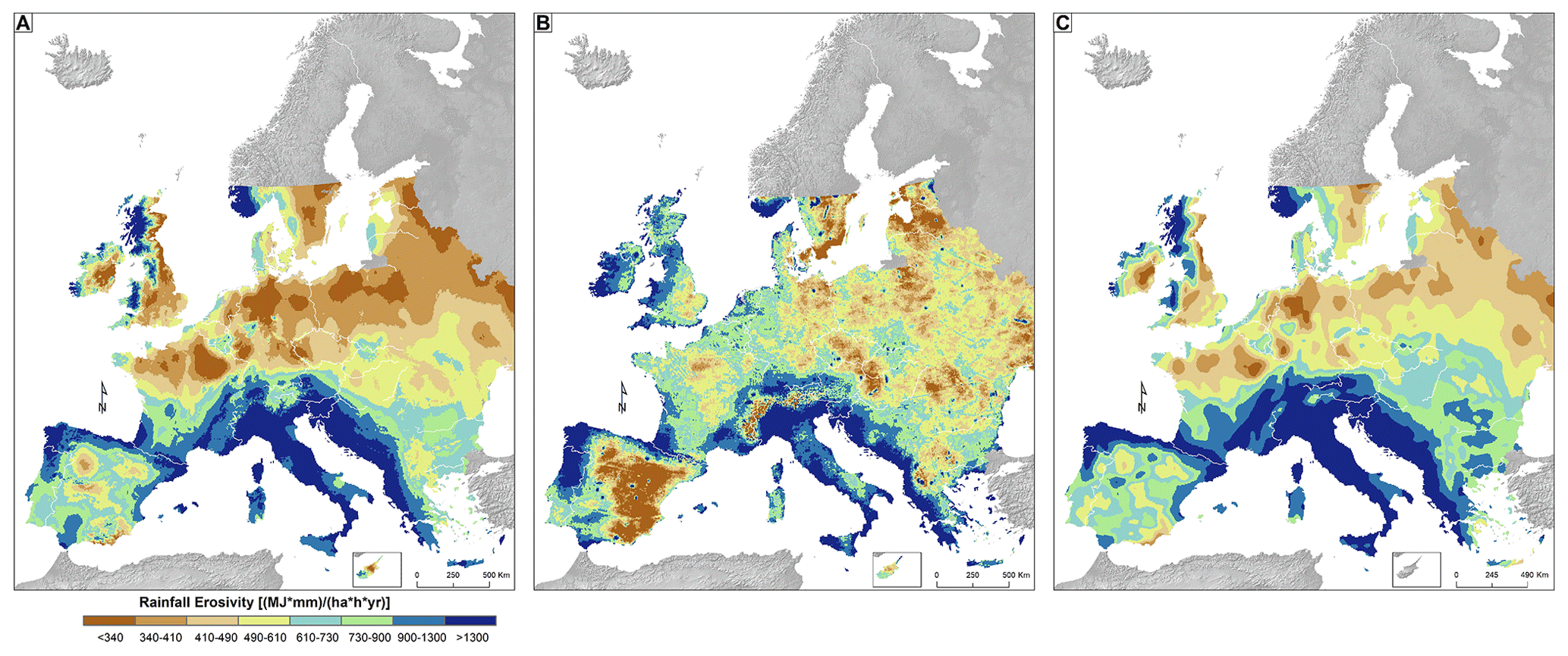
Figure 6Comparison between the GloREDa rainfall erosivity map prepared by Panagos et al. (2017) (a), the CMORPH-derived rainfall erosivity map (b), and the ED-concept-derived map (c) for Europe.
Table 4Comparison between monthly rainfall erosivity characteristics for Europe using Ballabio et al. (2017), the ED concept, and the CMOPRH product.
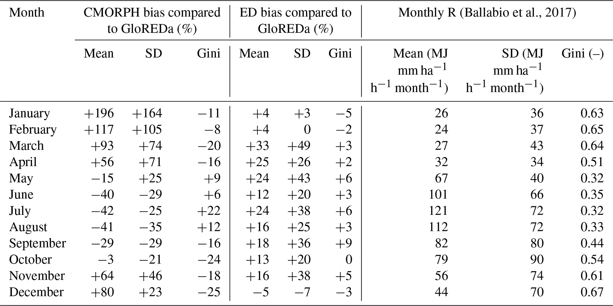
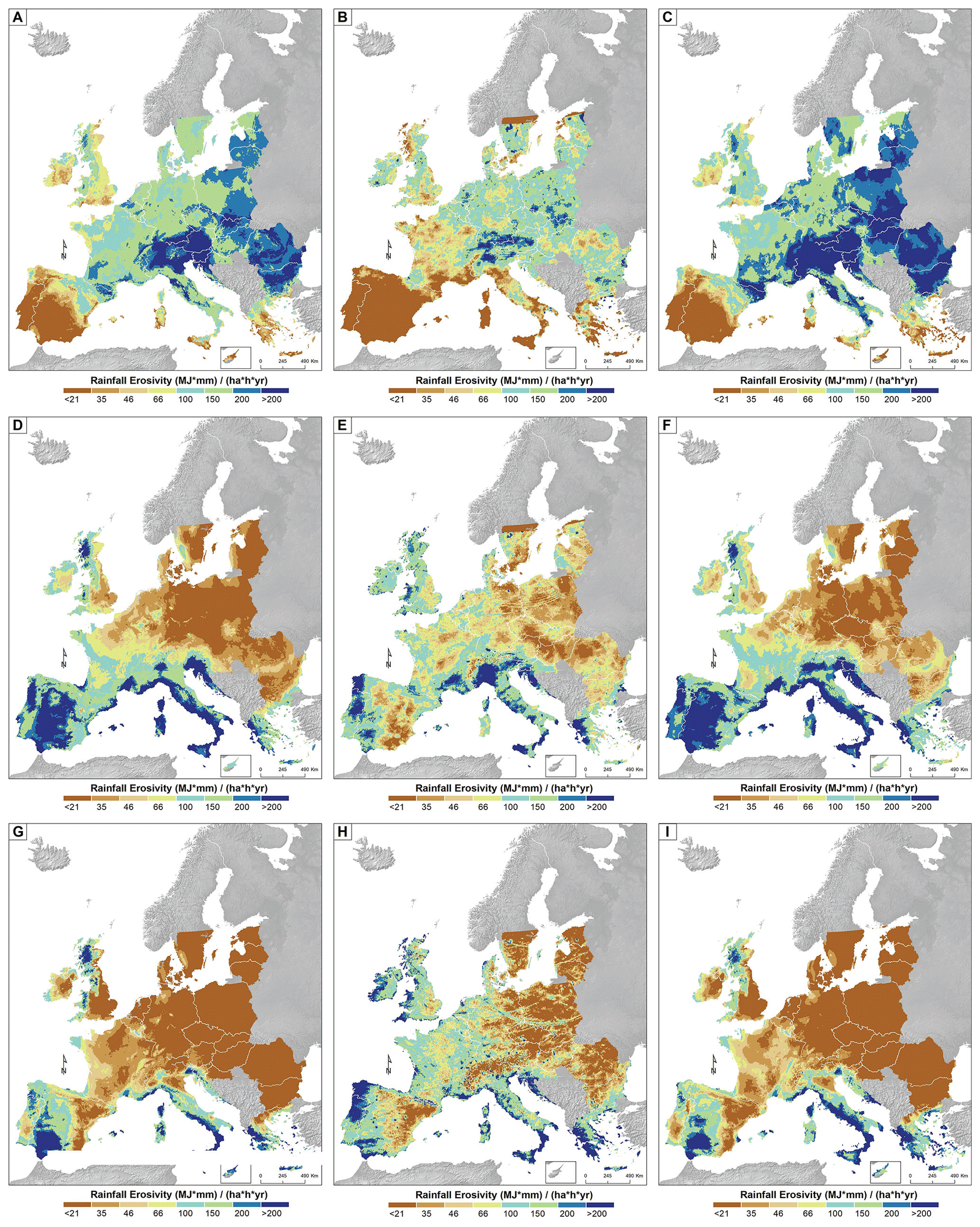
Figure 7Comparison between monthly erosivity maps for Europe prepared by the Ballabio et al. (2017) (a, d, g), CMORPH (b, e, h), and ED concept (c, f, i) maps for July (a, b, c), October (d, e, f), and December(g, h, i).
3.3.3 Comparison at the local scale using GloREDa stations
The station data of GloREDa were also compared to grid cell values at the same location from the derived CMORPH and ED rainfall erosivity maps. The Pearson correlation coefficient between the CMORPH and GloREDa data sets was equal to 0.74 (R2=0.55 with p value <0.01), and the mean bias was equal to −32 % (Fig. 8). In general, the CMORPH product yielded smaller rainfall erosivity estimates, especially for locations where annual rainfall erosivity exceeded 5000 MJ mm ha−1 h−1 yr−1 (Fig. 8). Additionally, CMORPH products tended to overestimate rainfall erosivity in locations near water bodies, which are also the points located above the orange line shown in Fig. 8. A comparison between the ED concept and GloREDa yielded a Pearson correlation coefficient of 0.77 (R2=0.59 with p value <0.01) and a mean bias of 10 %. Similarly, better agreement between the ED concept and GloREDa was detected at a global, continental, or large catchment scales compared to CMORPH versus GloREDa.
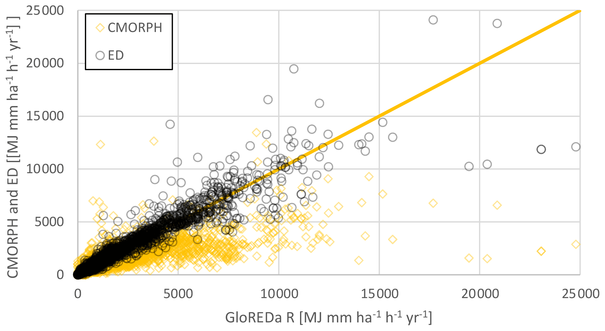
Figure 8Comparison between local (i.e., grid cell values) long-term annual rainfall erosivity from CMORPH and ED and stations' values of GloREDa.
3.4 CMORPH data correction using GloREDa point data
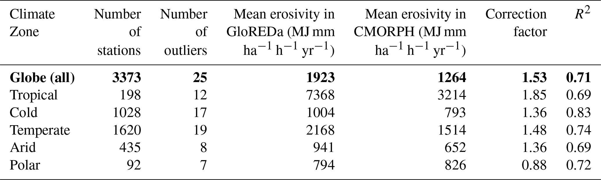
Considering the results and comparisons presented above, the attempt to adjust the CMORPH rainfall erosivity estimates using the estimates of the GloREDa ground station database was made. A similar attempt was also made by Kim et al. (2020) and Wang et al. (2020). In the scope of this study, we developed correction factors (or functions) for each of the Köppen–Geiger climate zones (Peel et al., 2007). The corrections were made both at a global scale using all GloREDa stations and per climate zone (Fig. 9). In Table 5, we propose the best linear function, which can be applied at CMORPH-estimated values in order to be as close as possible to the measured rainfall erosivity values of GloREDa.
Table 5Correction factors that were developed based on the GloREDa–CMORPH relationship per climate zone. R2 is the coefficient of determination. Bold text shows global area.
Therefore, a generic correction linear function that can be used to derive the corrected CMORPH data (CMORPHCOR) for the whole globe can be written as follows:
From the results of comparing GloREDa to CMORPH, it is evident that CMORPH underestimates the rainfall erosivity for a factor close to 2 (1.85) in tropical areas where we estimate a high R factor (Panagos et al., 2017). In temperate areas where the R factor is close to the global mean, the CMORPH underestimation is about 1.5, while better agreement can be seen in low-erosivity areas (arid, cold) (Fig. 9). Thus, applying this simple linear transformation can yield better agreement between GloREDa and CMORPHCOR, both at a station scale (Fig. 9) as well as at a global scale (Fig. S2). The same correction was also applied to the global rainfall erosivity map derived using the CMORPH product (Fig. S2) and yielded a global mean rainfall erosivity of 2000 MJ mm ha−1 h−1 yr−1 with a standard deviation of 3314 MJ mm ha−1 h−1 yr−1. Even if one notices much better agreement between CMORPHCOR and GloREDa after the correction, this is relevant only for long-term mean rainfall erosivity assessments. With regard to dynamic rainfall erosivity maps (i.e., for specific years or months), different correction factors should be applied based on the relationship between CMORPH and station rainfall erosivity for specific years. It is worth mentioning that the applied correction can be regarded as a relatively simple one, which could be suitable for global-scale modeling applications. By applying a correction factor to CMORPH, we aim to provide a simple method that uses available remote-sensing data to develop dynamic erosivity values.

Figure 9Comparison between CMORPH and GloREDa data sets at station scale and proposed correction factors for the whole data set and per climate zone (tropical, cold, temperate, arid, polar). Blue line indicates the linear trend. Red dots are the few outliers (i.e., identified based on Cook's distance) excluded from the correlation.
3.5 Temporal global erosivity trends for the period 1998–2019
The Mann–Kendall test was applied to identify areas with statistically significant (i.e., with a 0.05 significance level) changes (Fig. S3) during the period 1998–2019. According to CMORPH erosivity output, 15 % of the globe has a statistically significant change (Fig. S3). In case of the detected changes, most of the regions show a positive trend rather than a negative one according to the CMORPH product (Fig. S3). Therefore, the positive trend covers 80 % of the area where statistically significant change was detected (i.e., around 12 % of the total area) (Fig. S3), while the remaining 20 % (3 % of the total area) has a negative trend.
On the other hand, the ED concept yielded different results, as around 13 % of the total area shows a statistically significant trend, with positive and negative trends having similar shares (i.e., around 6.5 % each). Consistent trends for using both methods (i.e., CMORPH and the ED concept) were estimated in parts of North America and Asia, while opposite trends were found in parts of Africa, Asia, and Europe. A direct comparison to the study conducted by Bezak et al. (2020) that investigated rainfall erosivity trends in Europe (1961–2018) was not possible since the investigated periods did not overlap.
The global mean annual rainfall erosivity derived by Panagos et al. (2017) totals about 2190 MJ mm ha−1 h−1 yr−1 (i.e., the initial 1 km cell size map), with a standard deviation of 2974 MJ mm ha−1 h−1 yr−1. The area covered by CMORPH is slightly smaller (between the 60∘ S and 60∘ N parallels) than the one covered by the GloREDa map (between the 60∘ N and ∼75∘ N parallels, including some parts of Scandinavia, Siberia, and Canada). However, a GloREDa global mean rainfall erosivity value of about 1.8 times higher than the one derived based on the CMORPH data (shown in Sect. 3.1) cannot be explained by the slight difference between the two study areas. It should be noted that Kim et al. (2020) also reported that the CMORPH-derived rainfall erosivity was 1.65 lower than the GloREDa estimates (Panagos et al., 2017) for the United States of America (USA), with some USA regions showing a bias smaller than −80 % (Kim et al., 2020). More specifically, Kim et al. (2020) reported a mean annual value of 1260 MJ mm ha−1 h−1 yr−1 for the USA, while in this study a mean value of 1173 MJ mm ha−1 h−1 yr−1 was calculated using a slightly different methodology (e.g., a different eb−I equation was applied) and different time period. As the station density was quite low in the case of Panagos et al. (2017) study for Africa and North America and also parts of Asia, this can partly explain the larger differences between CMORH and GloREDa. On the other hand, the largest number of stations was positioned in Europe and also parts of Asia (Panagos et al., 2017), where the agreement between CMORPH and GloREDa was the best (Table 3). Thus, part of the differences between CMORPH and GloREDa can be attributed to the station density used by GloREDa and partly to the issues related to the detection of rainfall by the satellite-based products in mountainous regions (e.g., Stampoulis and Anagnostou, 2012).
In line with what was already discussed by Kim et al. (2020), the insights gained by conducting global analysis suggest that the CMORPH satellite-based rainfall erosivity estimates provide more seamless erosivity distribution without employing interpolation, uniform and good spatial coverage, and 30-time temporal resolution. However, it is also clear that this product has important disadvantages, i.e., overestimated precipitation over water bodies, that detection accuracy in hilly terrains can be problematic, that the accuracy of annual precipitation can be low, and that relative bias at event scale can be significant.
As previously noted, several studies have indicated that the difference between satellite-based products and ground-based precipitation data can be quite significant (Habib et al., 2012; Haile et al., 2015; Jiang et al., 2018). The differences in the rainfall intensity patterns can also be transformed into rainfall erosivity patterns. There were numerous studies published that investigated the accuracy of the CMORPH product in terms of precipitation. For example, Islam et al. (2020) showed that CMORPH overestimated the daily precipitation amount in Australia. A similar conclusion was made by An et al. (2020) for the Yellow River in China or by Wei et al. (2018) for mainland China. Some studies also showed a significant underestimation of CMORPH in winter seasons (Gebregiorgis and Hossain, 2015). Additionally, Palharini et al. (2020) showed that satellite-based products tended to underestimate extreme precipitation, which can have an important effect on rainfall erosivity. Underestimation of extreme rainfall events was also reported in many other studies (Jiang et al., 2019; Rahmawati and Lubczynski, 2018; Stampoulis et al., 2013; Sunilkumar et al., 2015; Wei et al., 2018b). This kind of underestimation can also lead to a negative bias of the satellite-based products compared to the station-based rainfall erosivity. Moreover, Tian et al. (2009) also showed that, in the USA, overestimation was seen for summer (i.e., overestimation of heavy precipitation with an intensity over 40 mm d−1) and underestimation for winter (i.e., missing a significant amount of light precipitation with an intensity lower than 10 mm d−1). Tian et al. (2009) also found out that hit bias (i.e., with respect to satellite-based data and reference data reporting precipitation coincidently) and missed precipitation were the two dominant error sources. A similar conclusion was also made by Jiang et al. (2018), who pointed out the limited detection accuracy of summer thunderstorms by the CMOPRH product in the Shanghai region. These drawbacks of CMORPH can also lead to underestimation or overestimation of the rainfall erosivity by CMORPH. Comparing the CMORPH outputs to the GloREDa-measured erosivity values for almost 3400 ground stations, we found that CMORPH underestimates erosivity in tropical areas by a factor close to 2, while there is better agreement for low-erosivity areas (cold, arid, polar). For the temperate climatic regions, CMORPH underestimates erosivity by a factor close to 1.5.
On the other hand, the only study that, to the best of the authors' knowledge, investigated this satellite-based derived rainfall erosivity (Kim et al., 2020) showed that CMORPH underestimated rainfall erosivity in the USA compared to the GloREDa map. Thus, it is clear that underestimation of the most extreme rainfall events can lead to large differences in the derived rainfall erosivity map. Such characteristics can also lead to relatively large differences in case satellite products are used for flood investigations (Dis et al., 2018). Underestimation of the precipitation amount by the CMOPRH product in southern Europe as shown in the Results section was also indicated by some other studies (Skok et al., 2016). Furthermore, Stampoulis and Anagnostou (2012) also pointed out that satellite-based precipitation product accuracy tended to be lower over the mountainous regions such as the Alpine region (or Andes). This was especially evident during the cold season (Stampoulis and Anagnostou, 2012) and was also highlighted in some other studies (Kidd et al., 2012). Also, other studies pointed a detection problem for winter precipitation and high-intensity rainfall events in some parts of Europe (Stampoulis and Anagnostou, 2012).
Different examples of good and worse agreement among presented rainfall erosivity maps can be seen around the globe (Figs. 4 and 5). Comparing the three maps (i.e., GloREDa, CMORPH, and ED) for parts of eastern Europe and Turkey (Fig. 4), relatively good agreement between all three maps was detected. The main reasons for this good agreement are (a) the relatively large number of stations with a measured R factor which contributed to the GloREDa map in countries such as Romania or Turkey (Panagos et al., 2017), (b) the relatively flat terrain without major mountainous regions in parts of eastern Europe, and (c) the relatively low-medium erosivity (<1000 MJ mm ha−1 h−1 yr−1). By contrast, there are many regions where differences are much larger. An example is the Andes mountain region (Fig. 5), where GloREDa includes only 15 stations in the central part of Chile (Panagos et al., 2017) and gridded precipitation products such as WorldClim also underestimate precipitation (Beck et al., 2020).
The ED (based on the ERA5 and GloREDa data) rainfall erosivity estimates showed better agreement with the GloREDa point estimates, which could be regarded as an expected result due to the selected input data. The largest differences between the ED and the GloREDa estimates were observed in Asia, Europe, and South America because of the precipitation underestimation in mountainous regions such as the Andes, Himalayas, and Alps (Beck et al., 2020). The deviation of ED compared to the GloREDa map could be explained by two main reasons: (a) the difference in the spatial resolution of the GloREDa and CMORPH maps as aggregating the 1 km GloREDa map to the 0.25∘ that is used by ERA5 yielded a global mean value of 2329 MJ mm ha−1 h−1 yr−1 and that (b) the WorldClim V1 map that was used as input to produce the GloREDa map underestimates the precipitation and that the updated version of the WorldClim map (i.e., V2) yields around 10 % higher annual global precipitation (Beck et al., 2020). It should be noted that the ED concept indirectly uses the GloREDa data for the estimation.
ED has the following advantages compared to the CMORPH approach: (a) the ED concept can be used to prepare dynamic rainfall erosivity maps that have better agreement with GloREDa, and (b) there are no issues with the accuracy near water bodies. On the other hand, ED also has some shortcomings: (a) most of the gridded precipitation data sets underestimate precipitation over mountain regions (Beck et al., 2020) and (b) consider the erosivity–precipitation relationship to be constant, and (c) the rainfall erosivity map is needed as input.
The density of stations used to produce the GloREDa map is locally low, especially in the African and South American continents. Obviously, this could have a substantial effect on the produced global rainfall erosivity map (Panagos et al., 2017) and consequently on the results presented in this study since the GloREDa map was used here as a reference. However, to the best of the authors' knowledge, GloREDa is the only global assessment using hourly and sub-hourly rainfall data and the best performing among the global assessments currently available (Panagos et al., 2017). This is due to the coarser time step of other potential global rainfall erosivity sources (Liu et al., 2020). Since the ED concept directly uses the GloREDa map, the results produced by the ED method are directly influenced by the potential shortcomings of GloREDa, and this should be taken into account when making further applications using the ED.
On the other hand, the satellite-based precipitation products have their own sources of uncertainty, as highlighted in the previous sections, and, consequently, CMORH significantly underestimates global rainfall erosivity rates compared to GloREDa. It should be noted that there are other potential products that could have been used to produce global rainfall erosivity maps and that could perhaps yield better results than CMORPH. For example, Multi-Source Weighted-Ensemble Precipitation (MSWEP) uses gauge, reanalysis, and satellite data sources, and it was shown that it outperforms some other products such as CMORPH (Beck et al., 2019a, b). Its spatial resolution is 0.1∘, and it is available from 1979. Moreover, the Tropical Rainfall Measuring Mission (TRMM) rainfall products can also be used to derive the rainfall erosivity (Li et al., 2020). However, it should be noted that the temporal resolution of these two products is 3 h, which requires a non-standard RUSLE approach to derive the rainfall erosivity (Renard et al., 1997). Thus, alternative approaches for rainfall erosivity estimation are needed. For example, Li et al. (2020) used a modified Brown and Foster equation to calculate the specific kinetic energy and consequently the rainfall kinetic energy. However, this equation was developed based on the case study from China and can therefore be regarded as a local (not global) equation. Thus, applying this equation to the global scale could introduce additional uncertainty to the results. Furthermore, one could also apply the correction (i.e., conversion) factor that was suggested by Panagos et al. (2016b). However, a relatively high value is obtained for the 3 h duration (i.e., a value of 6.6), and the equation used to calculate the conversion factors was only developed for durations up to 1 h. Therefore, applying the correction factors developed by Panagos et al. (2016b) could lead to uncertain results. Thus, there is no globally accepted method for the calculation of the global rainfall erosivity using the 3 h data set. Moreover, these two products also have coarser spatial resolution compared to CMORPH, which also affects the detection of the most extreme rainfall events. Other potential sources (e.g., reanalysis, satellite-based, or combined) with a different temporal and spatial resolution could be additionally tested (Beck et al., 2019a).
The global rainfall erosivity was assessed using the CMORPH product and the ED concept. To the best of the authors' knowledge, high temporal (30 min) and spatial resolution satellite-based products such as CMORPH have not yet been used for the development of global rainfall erosivity maps. Past attempts to develop a global erosivity data set based on satellite-based or reanalysis products have used either monthly or daily data. The comparison of the derived maps was performed at global and multiple regional scales using annual and monthly rainfall erosivity values.
The CMORPH product leads to a marked underestimation of annual rainfall erosivity across the globe, with an average value of 1.53 times lower than the GloREDa station-based rainfall erosivity. The agreement between CMORPH and GloREDa estimates varied significantly among continents and climatic zones. While the best agreement was detected for Europe (i.e., percent bias around 10 %), on average, it has relatively low-erosivity values, and a considerably lower performance was observed for Africa and South America (i.e., percent bias around −60 %). Besides having a higher average rainfall erosivity value than Europe, these regions also suffer from a considerably lower number of measurement stations in the GloREDa database. Interpretation of the obtained results suggested that satellite-based products such as CMORPH cannot correctly capture the most extreme rainfall events that contribute to the largest proportion of the annual rainfall erosivity in some parts of the globe. Better agreement was generally detected between the ED concept and GloREDa (i.e., percent bias up to around 20 %), which can be regarded as an expected result since the ED concept indirectly uses the information from GloREDa.
A more detailed comparison was performed for Europe, where an investigation was also performed at a monthly timescale. Some spatial erosivity patterns were well detected by the CMORPH product in some regions, and monthly erosivity values in spring and fall were relatively close to the ones reported by the monthly erosivity maps prepared by Ballabio et al. (2017) (e.g., in parts of eastern and central Europe). Additionally, underestimation and overestimation were detected in summer (percent bias up to −40 %) and winter (percent bias up to 100 %) compared to GloREDa, respectively. On the other hand, the ED concept consistently slightly overestimated GloREDa but yielded better agreement with GloREDa both temporally and spatially than CMORPH (i.e., percent bias was in the range of around 30 %). As mentioned, the ED approach indirectly uses the GloREDa information, but it is to some extent independent as it uses a completely different rainfall data set (i.e., ERA5 instead of WorldClim).
We also estimated a temporal trend analysis at a global scale using high temporal and spatial resolution data of CMORPH for the period 1998–2019. A preliminary trend investigation revealed that around 15 % of the investigated area was characterized by the statistically significant change in the annual rainfall erosivity, while around 80 % of this change was positive (i.e., 12 % of the total area) according to the CMORPH product for the 1998–2019 period. According to the ED concept, 13 % of the area was characterized by a statistically significant trend. In some regions (e.g., parts of South or North America), the detected trends were consistent, while others were not consistent (e.g., parts of Africa or Asia). Thus, detected trends according to CMORPH could indicate that rainfall erosivity has been slightly increasing in 12 % of the globe during the last 2 decades. However, a more detailed investigation using longer time series is needed to confirm or reject this preliminary result.
It should be noted that in case the CMORPH product is used for the preparation of the rainfall erosivity map, it would be further used for soil erosion modeling where an uncertainty assessment should be included in such an investigation, similar to some other scientific disciplines (e.g., Kim et al., 2016; Sun et al., 2018).
Despite the mentioned shortcomings and strong underestimation of the rainfall erosivity in some parts of the globe, the satellite-based precipitation products tend to be an interesting option for the estimation of the rainfall erosivity, especially in regions with limited ground data. However, in some regions and seasons, such products require additional correction to remove bias, which is of course related to the availability of ground-based precipitation. Thus, it is clear that such ground-based high-frequency precipitation measurements are (still) essential for accurate rainfall erosivity estimates; however, one can expect that technological development in the next decades will lead to improved accuracy (Tang et al., 2020) of satellite-based products such as CMORPH. These kinds of products could be used as an input to the dynamic soil erosion models, which could be used by relevant stakeholders. At the moment, alternative approaches such as the ED concept can provide more accurate rainfall erosivity estimates, which can be computed more easily.
The CMORPH data can be downloaded at https://www.ncei.noaa.gov/data/cmorph-high-resolution-global-precipitation-estimates/access/ (NOAA, 2022). ERA5 was downloaded through Copernicus CDS (https://doi.org/10.24381/cds.bd0915c6, Hersbach et al., 2018). Rainfall erosivity products were derived from https://esdac.jrc.ec.europa.eu/resource-type/datasets (Panagos et al., 2012). R code can be obtained upon request from the corresponding author.
The supplement related to this article is available online at: https://doi.org/10.5194/hess-26-1907-2022-supplement.
All the authors developed the concepts of the manuscript, and NB conducted calculations and wrote the first draft. PB and PP edited and improved the manuscript and figures.
The contact author has declared that neither they nor their co-authors have any competing interests.
Publisher’s note: Copernicus Publications remains neutral with regard to jurisdictional claims in published maps and institutional affiliations.
We thank Leonidas Liakos for his contribution to the statistical analysis in the development of the correction factors. Mark Bryan Alivio's support with English editing is also highly appreciated. We also thank the NOAA for providing the global bias-corrected CMORPH CDR rainfall data and the ECMWF, who made available the ERA5 data set. The critical and useful comments of two anonymous reviewers and the editor greatly improved the manuscript.
Nejc Bezak is grateful for the support of the Slovenian Research Agency (ARRS) through grant no. P2-0180 and the support from the UNESCO Chair on Water-related Disaster Risk Reduction. Pasquale Borrelli is funded by the EcoSSSoil Project, Korea Environmental Industry & Technology Institute (KEITI), Korea (grant no. 2019002820004).
This paper was edited by Yue-Ping Xu and reviewed by two anonymous referees.
Aghakouchak, A., Mehran, A., Norouzi, H., and Behrangi, A.: Systematic and random error components in satellite precipitation data sets, Geophys. Res. Lett., 39, L09406, https://doi.org/10.1029/2012GL051592, 2012.
An, Y., Zhao, W., Li, C., and Liu, Y.: Evaluation of Six Satellite and Reanalysis Precipitation Products Using Gauge Observations over the Yellow River Basin, China, Atmosphere, 11, 1–20, https://doi.org/10.3390/atmos11111223, 2020.
Angulo-Martínez, M. and Beguería, S.: Trends in rainfall erosivity in NE Spain at annual, seasonal and daily scales, 1955–2006, Hydrol. Earth Syst. Sci., 16, 3551–3559, https://doi.org/10.5194/hess-16-3551-2012, 2012.
Ballabio, C., Borrelli, P., Spinoni, J., Meusburger, K., Michaelides, S., Beguería, S., Klik, A., Petan, S., Janeček, M., Olsen, P., Aalto, J., Lakatos, M., Rymszewicz, A., Dumitrescu, A., Tadić, M. P., Diodato, N., Kostalova, J., Rousseva, S., Banasik, K., Alewell, C., and Panagos, P.: Mapping monthly rainfall erosivity in Europe, Sci. Total Environ., 579, 1298–1315, https://doi.org/10.1016/J.SCITOTENV.2016.11.123, 2017.
Beck, H. E., Pan, M., Roy, T., Weedon, G. P., Pappenberger, F., van Dijk, A. I. J. M., Huffman, G. J., Adler, R. F., and Wood, E. F.: Daily evaluation of 26 precipitation datasets using Stage-IV gauge-radar data for the CONUS, Hydrol. Earth Syst. Sci., 23, 207–224, https://doi.org/10.5194/hess-23-207-2019, 2019a.
Beck, H. E., Wood, E. F., Pan, M., Fisher, C. K., Miralles, D. G., Van Dijk, A. I. J. M., McVicar, T. R., and Adler, R. F.: MSWep v2 Global 3-hourly 0.1∘ precipitation: Methodology and quantitative assessment, B. Am. Meteorol. Soc., 100, 473–500, https://doi.org/10.1175/BAMS-D-17-0138.1, 2019b.
Beck, H. E., Wood, E. F., McVicar, T. R., Zambrano-Bigiarini, M., Alvarez-Garreton, C., Baez-Villanueva, O. M., Sheffield, J., and Karger, D. N.: Bias correction of global high-resolution precipitation climatologies using streamflow observations from 9372 catchments, J. Climate, 33, 1299–1315, https://doi.org/10.1175/JCLI-D-19-0332.1, 2020.
Bezak, N., Ballabio, C., Mikoš, M., Petan, S., Borrelli, P., and Panagos, P.: Reconstruction of past rainfall erosivity and trend detection based on the REDES database and reanalysis rainfall, J. Hydrol., 590, 125372, https://doi.org/10.1016/j.jhydrol.2020.125372, 2020.
Bezak, N., Borrelli, P., and Panagos, P.: A first assessment of rainfall erosivity synchrony scale at pan-European scale, Catena, 198, 105060, https://doi.org/10.1016/j.catena.2020.105060, 2021.
Borrelli, P., Robinson, D. A., Fleischer, L. R., Lugato, E., Ballabio, C., Alewell, C., Meusburger, K., Modugno, S., Schütt, B., Ferro, V., Montanarella, L., and Panagos, P.: An assessment of the global impact of 21st century land use change on soil erosion, Nat. Commun., 8, 2013, https://doi.org/10.1038/s41467-017-02142-7, 2017.
Borrelli, P., Robinson, D. A., Panagos, P., Lugato, E., Yang, J. E., Alewell, C., Wuepper, D., Montanarella, L., and Ballabio, C.: Land use and climate change impacts on global soil erosion by water (2015–2070), P. Natl. Acad. Sci. USA, 117, 21994–22001, https://doi.org/10.1073/pnas.2001403117, 2020.
Brown, L. C. and Foster, G.: Storm erosivity using idealised intensity distribution, T. ASAE, 30, 379–386, https://doi.org/10.13031/2013.31957, 1987.
Burn, D. H. and Hag Elnur, M. A.: Detection of hydrologic trends and variability, J. Hydrol., 255, 107–122, https://doi.org/10.1016/S0022-1694(01)00514-5, 2002.
Carollo, F. G., Ferro, V., and Serio, M. A.: Reliability of rainfall kinetic power–intensity relationships, Hydrol. Process., 31, 1293–1300, https://doi.org/10.1002/hyp.11099, 2017.
Chen, H., Chandrasekar, V., Cifelli, R., and Xie, P.: A Machine Learning System for Precipitation Estimation Using Satellite and Ground Radar Network Observations, IEEE Trans. Geosci. Remote Sens., 58, 982–994, https://doi.org/10.1109/TGRS.2019.2942280, 2020.
Chen, Y., Xu, M., Wang, Z., Gao, P., and Lai, C.: Applicability of two satellite-based precipitation products for assessing rainfall erosivity in China, Sci. Total Environ., 757, 143975, https://doi.org/10.1016/j.scitotenv.2020.143975, 2021.
Cui, Y., Pan, C., Liu, C., Luo, M., and Guo, Y.: Spatiotemporal variation and tendency analysis on rainfall erosivity in the Loess Plateau of China, Hydrol. Res., 51, 1048–1062, https://doi.org/10.2166/nh.2020.030, 2020.
Dabney, S. M., Yoder, D. C., and Vieira, D. A. N.: The application of the Revised Universal Soil Loss Equation, Version 2, to evaluate the impacts of alternative climate change scenarios on runoff and sediment yield, J. Soil Water Conserv., 67, 343–353, https://doi.org/10.2489/jswc.67.5.343, 2012.
Diodato, N., Borrelli, P., Panagos, P., Bellocchi, G., and Bertolin, C.: Communicating Hydrological Hazard-Prone Areas in Italy With Geospatial Probability Maps, Front. Environ. Sci., 7, 193, https://doi.org/10.3389/fenvs.2019.00193, 2019.
Dis, M. O., Anagnostou, E., and Mei, Y.: Using high-resolution satellite precipitation for flood frequency analysis: case study over the Connecticut River Basin, J. Flood Risk Manag., 11, S514–S526, https://doi.org/10.1111/jfr3.12250, 2018.
Dodson, R. and Marks, D.: Daily air temperature interpolated at high spatial resolution over a large mountainous region, Clim. Res., 8, 61–73, https://doi.org/10.3354/cr008001, 1997.
dos Santos Silva, D. S., Blanco, C. J. C., dos Santos Junior, C. S., and Martins, W. L. D.: Modeling of the spatial and temporal dynamics of erosivity in the Amazon, Model. Earth Syst. Environ., 6, 513–523, https://doi.org/10.1007/s40808-019-00697-6, 2020.
ERA5: ERA5, https://doi.org/10.24381/cds.f17050d7, 2021.
Ganasri, B. P. and Ramesh, H.: Assessment of soil erosion by RUSLE model using remote sensing and GIS – A case study of Nethravathi Basin, Geosci. Front., 7, 953–961, https://doi.org/10.1016/j.gsf.2015.10.007, 2016.
Gebregiorgis, A. S. and Hossain, F.: How well can we estimate error variance of satellite precipitation data around the world?, Atmos. Res., 154, 39–59, https://doi.org/10.1016/j.atmosres.2014.11.005, 2015.
Ghajarnia, N., Daneshkar Arasteh, P., Liaghat, M., and Araghinejad, S.: Error analysis on PERSIANN precipitation estimations: Case study of Urmia Lake Basin, Iran, J. Hydrol. Eng., 23, 05018006-1, https://doi.org/10.1061/(ASCE)HE.1943-5584.0001643, 2018.
Gini, C.: On the measurement of concentration and variability of characters, Metron, 63, 3–38, 1914.
Habib, E., Haile, A. T., Tian, Y., and Joyce, R. J.: Evaluation of the high-resolution CMORPH satellite rainfall product using dense rain gauge observations and radar-based estimates, J. Hydrometeorol., 13, 1784–1798, https://doi.org/10.1175/JHM-D-12-017.1, 2012.
Haile, A. T., Yan, F., and Habib, E.: Accuracy of the CMORPH satellite-rainfall product over Lake Tana Basin in Eastern Africa, Atmos. Res., 163, 177–187, https://doi.org/10.1016/j.atmosres.2014.11.011, 2015.
Hamed, K. H.: Trend detection in hydrologic data: The Mann-Kendall trend test under the scaling hypothesis, J. Hydrol., 349, 350–363, https://doi.org/10.1016/j.jhydrol.2007.11.009, 2008.
Hersbach, H., Bell, B., Berrisford, P., Biavati, G., Horányi, A., Muñoz Sabater, J., Nicolas, J., Peubey, C., Radu, R., Rozum, I., Schepers, D., Simmons, A., Soci, C., Dee, D., and Thépaut, J.-N.: ERA5 hourly data on pressure levels from 1979 to present, Copernicus Climate Change Service (C3S) Climate Data Store (CDS), https://doi.org/10.24381/cds.bd0915c6, 2018.
Islam, M. A., Yu, B., and Cartwright, N.: Assessment and comparison of five satellite precipitation products in Australia, J. Hydrol., 590, 125474, https://doi.org/10.1016/j.jhydrol.2020.125474, 2020.
Jiang, Q., Li, W., Wen, J., Qiu, C., Sun, W., Fang, Q., Xu, M., and Tan, J.: Accuracy evaluation of two high-resolution satellite-based rainfall products: TRMM 3B42V7 and CMORPH in Shanghai, Water (Switzerland), 10, 40, https://doi.org/10.3390/w10010040, 2018.
Jiang, Q., Li, W., Wen, J., Fan, Z., Chen, Y., Scaioni, M., and Wang, J.: Evaluation of satellite-based products for extreme rainfall estimations in the eastern coastal areas of China, J. Integr. Environ. Sci., 16, 191–207, https://doi.org/10.1080/1943815X.2019.1707233, 2019.
Kidd, C., Bauer, P., Turk, J., Huffman, G. J., Joyce, R., Hsu, K.-L., and Braithwaite, D.: Intercomparison of high-resolution precipitation products over Northwest Europe, J. Hydrometeorol., 13, 67–83, https://doi.org/10.1175/JHM-D-11-042.1, 2012.
Kim, J., Han, H., Kim, B., Chen, H., and Lee, J.-H.: Use of a high-resolution-satellite-based precipitation product in mapping continental-scale rainfall erosivity: A case study of the United States, Catena, 193, 104602, https://doi.org/10.1016/j.catena.2020.104602, 2020.
Kim, J. P., Jung, I., Park, K. W., Yoon, S. K., and Lee, D.: Hydrological utility and uncertainty of multi-satellite precipitation products in the mountainous region of South Korea, Remote Sens., 8, 608, https://doi.org/10.3390/rs8070608, 2016.
Kinnell, P. I. A.: Event soil loss, runoff and the Universal Soil Loss Equation family of models: A review, J. Hydrol., 385, 384–397, https://doi.org/10.1016/j.jhydrol.2010.01.024, 2010.
Kinnell, P. I. A.: CLIGEN as a weather generator for RUSLE2, Catena, 172, 877–880, https://doi.org/10.1016/j.catena.2018.09.016, 2019.
Lehner, B. and Grill, G.: Global river hydrography and network routing: Baseline data and new approaches to study the world's large river systems, Hydrol. Process., 27, 2171–2186, https://doi.org/10.1002/hyp.9740, 2013.
Li, X., Li, Z., and Lin, Y.: Suitability of trmm products with different temporal resolution (3-hourly, daily, and monthly) for rainfall erosivity estimation, Remote Sens., 12, 1–21, https://doi.org/10.3390/rs12233924, 2020.
Liu, Y., Zhao, W., Liu, Y., and Pereira, P.: Global rainfall erosivity changes between 1980 and 2017 based on an erosivity model using daily precipitation data, Catena, 194, 104768, https://doi.org/10.1016/j.catena.2020.104768, 2020.
Lorenz, M. O.: Methods of measuring the concentration of wealth, Publ. Am. Stat. Assoc., 9, 209–219, https://doi.org/10.2307/2276207, 1905.
Masaki, Y., Hanasaki, N., Takahashi, K., and Hijioka, Y.: Global-scale analysis on future changes in flow regimes using Gini and Lorenz asymmetry coefficients, Water Resour. Res., 50, 4054–4078, https://doi.org/10.1002/2013WR014266, 2014.
McLeod, A. I.: Kendall rank correlation and Mann-Kendall trend test, 12, http://www.stats.uwo.ca/faculty/aim (last access: 10 January 2022), 2011.
Mineo, C., Ridolfi, E., Moccia, B., Russo, F., and Napolitano, F.: Assessment of rainfall kinetic-energy-intensity relationships, Water, 11, 1994, https://doi.org/10.3390/w11101994, 2019.
Nearing, M. A., Unkrich, C. L., Goodrich, D. C., Nichols, M. H., and Keefer, T. O.: Temporal and elevation trends in rainfall erosivity on a 149 km2 watershed in a semi-arid region of the American Southwest, Int. Soil Water Conserv. Res., 3, 77–85, https://doi.org/10.1016/j.iswcr.2015.06.008, 2015.
Nearing, M. A., Yin, S.-Q., Borrelli, P., and Polyakov, V. O.: Rainfall erosivity: An historical review, Catena, 157, 357–362, https://doi.org/10.1016/j.catena.2017.06.004, 2017.
Nel, W., Reynhardt, D. A., and Sumner, P. D.: Effect of altitude on erosive characteristics of concurrent rainfall events in the northern kwazulu-natal drakensberg, Water, 36, 509–512, 2010.
NOAA: CMORPH dataset, https://www.ncei.noaa.gov/data/cmorph-high-resolution-global-precipitation-estimates/access/, last access 28 March 2022.
Palharini, R. S. A., Vila, D. A., Rodrigues, D. T., Quispe, D. P., Palharini, R. C., de Siqueira, R. A., and de Sousa Afonso, J. M.: Assessment of the extreme precipitation by satellite estimates over South America, Remote Sens., 12, 2085, https://doi.org/10.3390/rs12132085, 2020.
Panagos, P., Van Liedekerke, M., Jones, A., and Montanarella, L.: European Soil Data Centre: Response to European policy support and public data requirements, Land Use Policy, 29, 329–338, https://doi.org/10.1016/j.landusepol.2011.07.003, 2012 (data available at: https://esdac.jrc.ec.europa.eu/resource-type/datasets, last access: 10 January 2022).
Panagos, P., Ballabio, C., Borrelli, P., Meusburger, K., Klik, A., Rousseva, S., Tadić, M. P., Michaelides, S., Hrabalíková, M., Olsen, P., Beguería, S., and Alewell, C.: Rainfall erosivity in Europe, Sci. Total Environ., 511, 801–814, https://doi.org/10.1016/j.scitotenv.2015.01.008, 2015.
Panagos, P., Borrelli, P., Spinoni, J., Ballabio, C., Meusburger, K., Beguería, S., Klik, A., Michaelides, S., Petan, S., Hrabalíková, M., Banasik, K., and Alewell, C.: Monthly rainfall erosivity: Conversion factors for different time resolutions and regional assessments, Water, 8, 119, https://doi.org/10.3390/w8040119, 2016a.
Panagos, P., Ballabio, C., Borrelli, P., and Meusburger, K.: Spatio-temporal analysis of rainfall erosivity and erosivity density in Greece, Catena, 137, 161–172, https://doi.org/10.1016/j.catena.2015.09.015, 2016b.
Panagos, P., Borrelli, P., Meusburger, K., Yu, B., Klik, A., Jae Lim, K., Yang, J. E., Ni, J., Miao, C., Chattopadhyay, N., Sadeghi, S. H., Hazbavi, Z., Zabihi, M., Larionov, G. A., Krasnov, S. F., Gorobets, A. V, Levi, Y., Erpul, G., Birkel, C., Hoyos, N., Naipal, V., Oliveira, P. T. S., Bonilla, C. A., Meddi, M., Nel, W., Al Dashti, H., Boni, M., Diodato, N., Van Oost, K., Nearing, M., and Ballabio, C.: Global rainfall erosivity assessment based on high-temporal resolution rainfall records, Sci. Rep., 7, 4175, https://doi.org/10.1038/s41598-017-04282-8, 2017.
Peel, M. C., Finlayson, B. L., and McMahon, T. A.: Updated world map of the Köppen-Geiger climate classification, Hydrol. Earth Syst. Sci., 11, 1633–1644, https://doi.org/10.5194/hess-11-1633-2007, 2007.
Petan, S., Rusjan, S., Vidmar, A., and Mikoš, M.: The rainfall kinetic energy-intensity relationship for rainfall erosivity estimation in the mediterranean part of Slovenia, J. Hydrol., 391, 314–321, https://doi.org/10.1016/j.jhydrol.2010.07.031, 2010.
Petek, M., Mikoš, M., and Bezak, N.: Rainfall erosivity in Slovenia: Sensitivity estimation and trend detection, Environ. Res., 167, 528–535, https://doi.org/10.1016/j.envres.2018.08.020, 2018.
Prakash, S.: Performance assessment of CHIRPS, MSWEP, SM2RAIN-CCI, and TMPA precipitation products across India, J. Hydrol., 571, 50–59, https://doi.org/10.1016/j.jhydrol.2019.01.036, 2019.
Prakash, S., Mitra, A. K., AghaKouchak, A., and Pai, D. S.: Error characterization of TRMM Multisatellite Precipitation Analysis (TMPA-3B42) products over India for different seasons, J. Hydrol., 529, 1302–1312, https://doi.org/10.1016/j.jhydrol.2015.08.062, 2015.
Rahmawati, N. and Lubczynski, M. W.: Validation of satellite daily rainfall estimates in complex terrain of Bali Island, Indonesia, Theor. Appl. Climatol., 134, 513–532, https://doi.org/10.1007/s00704-017-2290-7, 2018.
Reder, A. and Rianna, G.: Exploring ERA5 reanalysis potentialities for supporting landslide investigations: a test case from Campania Region (Southern Italy), Landslides, 1909–1924, https://doi.org/10.1007/s10346-020-01610-4, 2021.
Renard, K. G. and Freimund, J. R.: Using monthly precipitation data to estimate the R-factor in the revised USLE, J. Hydrol., 157, 287–306, https://doi.org/10.1016/0022-1694(94)90110-4, 1994.
Renard, K. G., Foster, G. R., Weesies, G. A., McCool, D. K., and Yoder, D. C.: Predicting Soil Erosion byWater: A Guide to Conservation Planning with the Revised Universal Soil Loss Equation (RUSLE) (Agricultural Handbook 703), US Department of Agriculture, ISBN 0-16-048938-5, 1997.
Rodrigues da Silva, V. D. P., Belo Filho, A. F., Rodrigues Almeida, R. S., de Holanda, R. M., and da Cunha Campos, J. H. B.: Shannon information entropy for assessing space-time variability of rainfall and streamflow in semiarid region, Sci. Total Environ., 544, 330–338, https://doi.org/10.1016/j.scitotenv.2015.11.082, 2016.
SAGA GIS: http://www.saga-gis.org/ (last access: 10 January 2022), 2021.
Sanchez-Moreno, J. F., Mannaerts, C. M., and Jetten, V.: Rainfall erosivity mapping for Santiago Island, Cape Verde, Geoderma, 217–218, 74–82, https://doi.org/10.1016/j.geoderma.2013.10.026, 2014.
Seo, B.-C., Krajewski, W. F., Quintero, F., ElSaadani, M., Goska, R., Cunha, L. K., Dolan, B., Wolff, D. B., Smith, J. A., Rutledge, S. A., Rutledge, S. A., and Petersen, W. A.: Comprehensive evaluation of the IFloodS Radar rainfall products for hydrologic applications, J. Hydrometeorol., 19, 1793–1813, https://doi.org/10.1175/JHM-D-18-0080.1, 2018.
Skok, G., Žagar, N., Honzak, L., Žabkar, R., Rakovec, J., and Ceglar, A.: Precipitation intercomparison of a set of satellite- and raingauge-derived datasets, ERA Interim reanalysis, and a single WRF regional climate simulation over Europe and the North Atlantic, Theor. Appl. Climatol., 123, 217–232, https://doi.org/10.1007/s00704-014-1350-5, 2016.
Stampoulis, D. and Anagnostou, E.: Evaluation of global satellite rainfall products over Continental Europe, J. Hydrometeorol., 13, 588–603, https://doi.org/10.1175/JHM-D-11-086.1, 2012.
Stampoulis, D., Anagnostou, E. N., and Nikolopoulos, E. I.: Assessment of high-resolution satellite-based rainfall estimates over the mediterranean during heavy precipitation events, J. Hydrometeorol., 14, 1500–1514, https://doi.org/10.1175/JHM-D-12-0167.1, 2013.
Sun, R., Yuan, H., and Yang, Y.: Using multiple satellite-gauge merged precipitation products ensemble for hydrologic uncertainty analysis over the Huaihe River basin, J. Hydrol., 566, 406–420, https://doi.org/10.1016/j.jhydrol.2018.09.024, 2018.
Sunilkumar, K., Narayana Rao, T., Saikranthi, K., and Purnachandra Rao, M.: Comprehensive evaluation of multisatellite precipitation estimates over India using gridded rainfall data, J. Geophys. Res., 120, 8987–9005, https://doi.org/10.1002/2015JD023437, 2015.
Sutanto, S. J., Vitolo, C., Di Napoli, C., D'Andrea, M., and Van Lanen, H. A. J.: Heatwaves, droughts, and fires: Exploring compound and cascading dry hazards at the pan-European scale, Environ. Int., 134, 105276, https://doi.org/10.1016/j.envint.2019.105276, 2020.
Tang, G., Clark, M. P., Papalexiou, S. M., Ma, Z., and Hong, Y.: Have satellite precipitation products improved over last two decades? A comprehensive comparison of GPM IMERG with nine satellite and reanalysis datasets, Remote Sens. Environ., 240, 111697, https://doi.org/10.1016/j.rse.2020.111697, 2020.
Teng, H., Ma, Z., Chappell, A., Shi, Z., Liang, Z., and Yu, W.: Improving rainfall erosivity estimates using merged TRMM and gauge data, Remote Sens., 9, 1134, https://doi.org/10.3390/rs9111134, 2017.
Tian, Y., Peters-Lidard, C. D., Eylander, J. B., Joyce, R. J., Huffman, G. J., Adler, R. F., Hsu, K., Turk, F. J., Garcia, M., and Zeng, J.: Component analysis of errors in satellite-based precipitation estimates, J. Geophys. Res.-Atmos., 114, D24101, https://doi.org/10.1029/2009JD011949, 2009.
Verstraeten, G., Poesen, J., Demarée, G., and Salles, C.: Long-term (105 years) variability in rain erosivity as derived from 10 min rainfall depth data for Ukkel (Brussels, Belgium): Implications for assessing soil erosion rates, J. Geophys. Res.-Atmos., 111, D22109, https://doi.org/10.1029/2006JD007169, 2006.
Wang, M., Yin, S., Yue, T., Yu, B., and Wang, W.: Rainfall erosivity estimation using gridded daily precipitation datasets, Hydrol. Earth Syst. Sci. Discuss. [preprint], https://doi.org/10.5194/hess-2020-633, 2020.
Wei, G., Lü, H., Crow, W. T., Zhu, Y., Wang, J., and Su, J.: Comprehensive evaluation of GPM-IMERG, CMORPH, and TMPA precipitation products with gauged rainfall over mainland China, Adv. Meteorol., 2018, 3024190, https://doi.org/10.1155/2018/3024190, 2018.
Xie, P., Joyce, R., Wu, S., Yoo, S.-H., Yarosh, Y., Sun, F., and Lin, R.: Reprocessed, bias-corrected CMORPH global high-resolution precipitation estimates from 1998, J. Hydrometeorol., 18, 1617–1641, https://doi.org/10.1175/JHM-D-16-0168.1, 2017.
Xie, P., Joyce, R., Yoo, S., Yarosh, S. H., Sun, Y., and Lin, F.: NOAA Climate Data Record (CDR) of CPC Morphing Technique (CMORPH) High Resolution Global Precipitation Estimates, Version 1, https://doi.org/10.25921/w9va-q159, 2021.
Yin, S., Nearing, M. A., Borrelli, P., and Xue, X.: Rainfall erosivity: An overview of methodologies and applications, Vadose Zone J., 16, 1–16, https://doi.org/10.2136/vzj2017.06.0131, 2017.
Yu, B. and Rosewell, C. J.: Rainfall erosivity estimation using daily rainfall amounts for South Australia, Aust. J. Soil Res., 34, 721–733, https://doi.org/10.1071/SR9960721, 1996.