the Creative Commons Attribution 4.0 License.
the Creative Commons Attribution 4.0 License.
 | 15 Mar 2022
Coastal and orographic effects on extreme precipitation revealed by weather radar observations
Moshe Armon
Efrat Morin
The yearly exceedance probability of extreme precipitation of multiple durations is crucial for infrastructure design, risk management, and policymaking. Local extremes emerge from the interaction of weather systems with local terrain features such as coastlines and orography; however, multi-duration extremes do not follow exactly the patterns of cumulative precipitation and are still not well understood. High-resolution information from weather radars could help us quantify their patterns better, but traditional extreme value analyses based on radar records were found to be too inaccurate for quantifying the extreme intensities required for impact studies. Here, we propose a novel methodology for extreme precipitation frequency analysis based on relatively short weather radar records, and we use it to investigate the coastal and orographic effects on extreme precipitation of durations between 10 min and 24 h. Combining 11 years of radar data with 10 min rain gauge data in the southeastern Mediterranean, we obtain estimates of the once in 100 years precipitation intensities with ∼26 % standard error, which is lower than those obtained using traditional approaches on rain gauge data. We identify the following three distinct regimes which respond differently to coastal and orographic forcing: short durations (∼10 min), related to peak convective rain rates, hourly durations (∼1 h), related to the yield of individual convective cells, and long durations (∼6–24 h), related to the accumulation of multiple convective cells and to stratiform processes. At short and hourly durations, extreme return levels peak at the coastline, while at longer durations they peak corresponding to the orographic barriers. The distributions tail heaviness is rather uniform above the sea and rapidly changes in presence of orography, with opposing directions at short (decreasing tail heaviness, with a peak at hourly durations) and long (increasing) durations. These distinct effects suggest that short-scale hazards, such as urban pluvial floods, could be more of concern for the coastal regions, while longer-scale hazards, such as flash floods, could be more relevant in mountainous areas.
- Article
(8065 KB) - Full-text XML
-
Supplement
(1904 KB) - BibTeX
- EndNote


Knowledge of the yearly exceedance probability of extreme precipitation intensities at multiple spatiotemporal scales is crucial for infrastructure design, weather risk management, and policymaking (Chow et al., 1988; Kleindorfer and Kunreuther, 1999). Typically, statistical models are fitted to the observed extremes and used to extrapolate design precipitation intensities corresponding to low yearly exceedance probabilities, which cannot be empirically quantified from observations. For example, the 100-year return levels are intensities characterized by 1 % yearly exceedance probability and, thus, exceeded on average once in 100 years (Katz et al., 2002). This task usually requires specific approaches to decrease the stochastic uncertainties characterizing the observation of extremes (e.g., Koutsoyiannis et al., 1988; Buishand, 1991; Burlando and Rosso, 1996) and simplified conceptual models to account for the multiple spatiotemporal scales required by many impact studies (Sivapalan and Bloeschl, 1998; Svensson and Jones, 2010).
Local precipitation climatology emerges from the interaction between weather systems and local terrain features. For instance, mountains constrain the flow of air masses inducing vertical motions which affect precipitation (Haiden et al., 1992; Houze et al., 2001; Roe, 2005). Similarly, sea–land interfaces and lakes may alter the precipitation characteristics due to the interaction of synoptic-scale winds with mesoscale features such as the sea/land breeze, the frictional-induced convergence associated with deceleration of wind speeds when air is blowing from sea inland, and the contribution of the coastal shape to convergence, with effects which can propagate far inland (Bergeron, 1949; Neumann, 1951; Bummer et al., 1995; Niziol et al., 1995; Colle and Yuter, 2007; Heiblum et al., 2011; Warner et al., 2012; Li and Carbone, 2015; Minder et al., 2015). While these phenomena are relatively well understood in terms of average precipitation yield, less is known about their impact on extreme precipitation intensities.
Extreme precipitation intensity does not follow exactly the patterns of cumulative precipitation. For example, the typical orographic enhancement of total precipitation was found to be reversed for extreme hourly precipitation (the reverse orographic effect), meaning that the hourly extremes tend to decrease with elevation (Allamano et al., 2009; Avanzi et al., 2015). The only study available so far on the orographic impact on sub-hourly design precipitation focused on the case of Mediterranean cyclones in the southeastern Mediterranean and found that orography tends to decrease the tail heaviness of precipitation intensity distribution, with a stronger effect at hourly durations with respect to sub-hourly or multi-hour durations (Marra et al., 2021b). As for the sea–land interfaces, extreme precipitation was found to be higher along narrow coastal regions (Mapes et al., 2003; Wu et al., 2009). For the southeastern Mediterranean, rain amounts defining the highest precipitation percentiles at sub-storm durations were found to be higher along the coastline, extending a few kilometers inland (Sharon and Kutiel, 1986; Karklinsky and Morin, 2006; Peleg and Morin, 2012; Armon et al., 2020). Nevertheless, with the exception of coarse-scale climatology from satellite-borne sensors, which, however, did not directly address the issue (Marra et al., 2017; Demirdjian et al., 2018; Courty et al., 2019), not much is known about the sea–land interactions in terms of extreme return levels, mostly due the obvious lack of in situ observations over the sea.
The interest in these questions is enhanced by ongoing climate change, which affects the hydrological cycle in yet unclear manners (Blöschl et al., 2019) and may result in a nonlinear response to natural hazards triggered by hydroclimatic extremes, such as urban floods (Arnbjerg-Nielsen et al., 2013), flash floods (Hicks et al., 2005; Amponsah et al., 2018), slope failures (Marchi et al., 2009; Paranunzio et al., 2019), forest disturbances (Ulbrich et al., 2001; Forzieri et al., 2020), and coastal flooding (Wahl et al., 2015; Bevacqua et al., 2019). An improved understanding of the interaction of weather systems with local terrain features and its effects on design precipitation intensities could help us better represent present and future extremes in impact studies (e.g., Attema and Lenderink, 2014; Peleg et al., 2020). However, information from in situ observations is often limited due to the large extension of ungauged regions worldwide (Kidd et al., 2017) and to the sparse representativeness of rain gauge sampling, which is particularly important in the case of short-duration extremes (Villarini et al., 2008; Peleg et al., 2018; Marra and Morin, 2018; Lengfeld et al., 2020).
Weather radars monitor regional scales over both land and sea with high spatial and temporal resolutions, providing fine-scale information on the spatial gradients of extreme intensities ranging from sub-hourly to sub-daily and daily durations (Collier, 1989; Saltikoff et al., 2019). They represent a unique opportunity to examine these local effects on the statistics of extreme precipitation, as they cover orographic regions more homogeneously than the typical rain gauge networks and offshore sea areas up to hundreds of kilometers from the coast (Kidd et al., 2017). The use of radar records for precipitation frequency analysis currently suffers from important uncertainties, mostly related to measurement errors (Eldardiry et al., 2015; Marra and Morin, 2015; McGraw et al., 2019) and to the use of statistical methods inadequate for the characteristics of weather radar records (Marra et al., 2019a). Most of the efforts so far focused on the reduction in these uncertainties (Overeem et al., 2009; Wright et al., 2013; Goudenhoofdt et al., 2017), so climatological analyses were only seldom attempted (Panziera et al., 2016; Marra et al., 2017).
Recent advances in the statistical description of extreme precipitation showed promising advantages over traditional approaches in estimating design precipitation intensities in the presence of problems typical of radar monitoring, such as short data records and measurement errors (Marani and Ignaccolo, 2015; Zorzetto et al., 2016; Marra et al., 2018). These novel methods were tested on satellite data with encouraging results (Zorzetto and Marani, 2019, 2020; Hu et al., 2020; Mekonnen et al., 2021), but, to the best of our knowledge, no weather radar application is available so far, with the exception of a single storm study case (Rinat et al., 2021).
Here, we exploit these novel statistical methods for precipitation frequency analysis to combine an 11-year weather radar archive covering the southeastern Mediterranean with data from a long-recording rain gauge network. We use this adjusted dataset to investigate the statistical characteristics of extreme precipitation emerging from the interaction of weather systems with coastal and orographic features. Specifically, we (a) devise and test a novel methodology to adjust radar-derived statistics based on in situ observations, and we use it to (b) investigate the coastal and orographic effects on the statistics of design extremes at multiple sub-daily durations. Using the new methodology, we find a notable impact of the coast on precipitation extremes and characterize differential orographic effects on extreme precipitation over sub-hourly to daily durations.
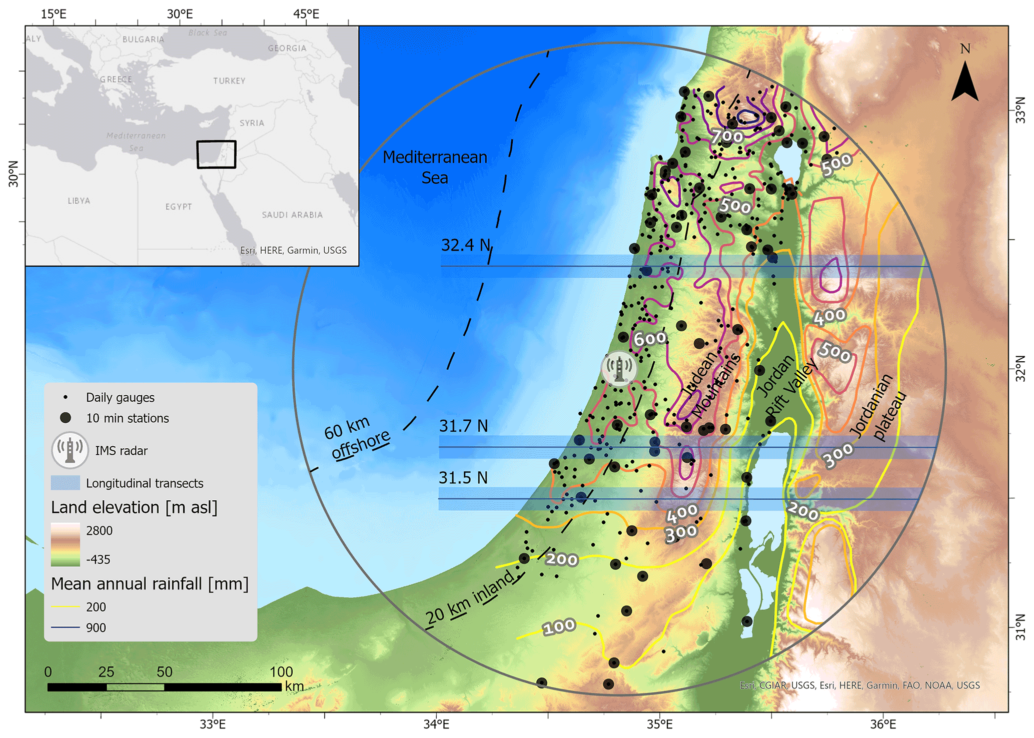
Figure 1Map of the study area showing the terrain elevation, location of the weather radar, 140 km range of the instrument, location of the daily rain gauges, location of the 10 min rain gauges, and locations of the three transects shown in Figs. 6 and 7. Mean annual rainfall is based on 1961–1990 rain gauge data (Enzel et al., 2003).
2.1 Study area
This study focuses on the region covered by the C-band weather radar of the Israel Meteorological Service (IMS) located at Beit Dagan, Israel (Fig. 1). The region shows a longitudinally organized physiography that, moving east from the Mediterranean Sea, encounters a coastal plain, an orographic barrier (Judaean Mountains; ∼1000 m a.s.l. – meters above sea level), a deep rift valley (Jordan Rift Valley; ∼400 m b.s.l. – meters below sea level), and a second orographic barrier (Jordanian plateau; >1000 m a.s.l.). Weather systems strongly interact with these rather regular orographic features generating steep gradients in precipitation climatology, which include drops in the mean annual amounts as high as ∼500 mm yr−1 within a distance of 25 km. Overall, precipitation amounts tend to increase with latitude and elevation and decrease with distance from the coast (Alpert and Shafir, 1989; Goldreich, 1994).
Precipitation is mostly brought by (i) Mediterranean cyclones (Ziv et al., 2015; Kushnir et al., 2017), (ii) low-pressure systems extending from the south (Red Sea troughs; de Vries et al., 2013), and (iii), more rarely, conveyor belts of moisture of tropical origin (tropical plumes; Rubin et al., 2007; Tubi and Dayan, 2014). Although these systems are characterized by distinct spatial and temporal scales and all potentially cause extreme precipitation (Marra et al., 2019b), Mediterranean cyclones are the dominant systems both in terms of number of wet days and total precipitation yield (∼75 %–90 % of total amounts), with the exception of the southern and eastern portions of the domain in which Red Sea troughs can contribute almost equally (Belachsen et al., 2017; Armon et al., 2018; Marra et al., 2019b). Mediterranean cyclones typically bring westerly winds from the Mediterranean Sea inland and, thus, interact with the coastal and orographic features of the area in a rather systematic way. Heavy precipitation processes are generally convective and characterized by high spatiotemporal variability, so rain gauge monitoring is often insufficient (Yakir and Morin, 2011; Peleg et al., 2013; Marra and Morin, 2018). Climate models project substantial changes in both the intensity and the occurrence of these systems (Hochman et al., 2018; Zappa et al., 2015), with complicated effects on compound extremes (Marra et al., 2019b, 2021a).
2.2 Rain gauge data
Rain gauge data were provided by the IMS and organized into two archives, namely the (i) daily archive, containing precipitation amounts measured every day at 06:00 UTC, used for the calibration and validation of the weather radar archive and for the definition of storms (see below), and the (ii) 10 min archive from automatic stations, containing data at 10 min temporal intervals and 0.1 mm tip resolution, used for the adjustment of radar-derived statistics at multiple temporal scales. All the data were quality controlled by the IMS; in addition, stations located in regions with low weather radar data quality (e.g., residual contamination by ground clutters and blockages) were removed to avoid negative impacts on the adjustments. In total, 437 daily stations and 65 10 min stations are used in the analyses (Fig. 1). Hydrological years (1 September to 31 August) with more than 10 % missing data were removed to ensure accurate quantification of the precipitation statistics (see Marra et al., 2020).
2.3 Weather radar data
A full re-elaboration of the weather radar archive was carried out to obtain a high-quality and homogeneous archive for the period 2007–2008 to 2017–2018. Physics-based corrections and empirical adjustments are combined in a procedure optimized for long-term radar archives and high-intensity convective storms (Marra et al., 2014; Marra and Morin, 2015, 2018). Non-precipitating echoes (i.e., ground clutters) are removed using a reparameterization of the filter by Jacobi et al. (2014; details in Marra and Morin, 2018). Beam blockage due to orography is corrected (up to 70 % power loss; Marra et al., 2014) using numerical simulations of the beam propagation in a digital elevation model (Pellarin et al., 2002). Non-orographic blockages are identified from the systematic power loss in long-term (yearly) observations and corrected by interpolation with nearby non-blocked beams. Beam attenuation in heavy rain is corrected with a modified Hitschfeld and Bordan (1954) algorithm using an upper limit of 10 dBZ to the correction factor (Marra and Morin, 2015); coefficients for convective environment are derived from Delrieu et al. (2000). Vertical variations in reflectivity are corrected based on spatially averaged profiles observed during 2 h windows, using the procedure in Marra and Morin (2015). Reflectivity is saturated at 59.5 dBZ to avoid contamination by hail. A fixed power law relation in the form , which was shown to be adequate for the convective precipitation of the region, is used to compute rain intensity (Morin and Gabella, 2007). Rain rate at the ground is obtained by averaging the two highest intensities along the vertical dimension for elevations up to 5∘ and is converted to a 500 m Cartesian grid. Bias adjustment is performed using the daily rain gauge archive and consists of two steps, i.e., a range-dependent adjustment based on yearly accumulations (Morin and Gabella, 2007) and an event-based mean field adjustment (Marra and Morin, 2015), with events defined as consecutive wet days (≥5 stations recording ≥0.1 mm; more details in Sect. 3.1).
A leave-one-out cross-validation of the archive at the daily scale shows a median fractional standard error (FSE; that is, the root mean square error normalized over the average rain gauge amount and computed as , where gi=1 … N are the rain gauge observations, and ri=1 … N are the radar estimates for the corresponding pixel, as in Marra and Morin, 2015) of 1.07 and a median correlation coefficient of 0.76 (see additional details in Fig. S1 in the Supplement). These metrics imply that the root mean square error of the daily amounts is 107 % of the average rain gauge daily amount in wet days (≥0.1 mm), and that ∼42 % of the variance is to be imputable to measurement errors. These results represent a large improvement over the previous radar archive available for the region, which had a correlation coefficient below 0.5 and FSE between 1.5 and 2 (Marra and Morin, 2015). These improvements are attributable to the more recent radar instrument and to the updated elaboration procedures, and motivate our choice of exploiting this shorter, but more accurate, archive in our study. The instrument was sometimes turned off so that the archive cannot be considered complete. Despite the evaluation metrics, some issues still remain in the final estimates, which could decrease the quantitative accuracy of the estimated return levels. For example, ground clutters in the first orographic range east of the radar can appear due to anomalous beam propagation, and some blocked beams could be not completely recovered, or they were over-filled by the correction, especially west of the instrument (e.g., see Figs. S1 and S2). In the eastern portion of the domain, the radar sample volumes are quite high in the atmosphere (due to the presence of the first orographic barrier), and no rain gauge is available for adjustment, leading to potential underestimation due to overshooting of the precipitation. Pixels located within 10 km of the instrument have been removed from the subsequent analyses to avoid the artifacts related to the suppression of side-lobe ground echoes. Underestimation due to range effects is also visible in the northern and southern portions of the domain for areas farther than ∼100 km from the radar.
3.1 Extreme value analysis
Design precipitation intensities are here quantified as return levels corresponding to low yearly exceedance probabilities. We use the framework for sub-daily precipitation frequency analysis based on the concept of ordinary events presented in Marra et al. (2020), and we rely on the simplified metastatistical extreme value (SMEV) method (Marra et al., 2019b) for the estimation of extreme return levels. Ordinary events are defined as all the independent realizations of a process of interest. Once the cumulative distribution function describing their tail, here termed the intensity distribution, is known, it is possible to compute an extreme value distribution to quantify intensities associated with rare yearly exceedance probabilities by explicitly considering their yearly occurrence frequency (Zorzetto et al., 2016). This approach is equivalent to ordinary statistics of n-sized block maxima under independence for which the tail behavior is known (Serinaldi et al., 2020). We define here the ordinary events' tail as the largest 45 % of the events, following the results in Marra et al. (2019b), which showed that values between 45 % and 20 % provide virtually indistinguishable results. We use a stretched exponential model (Weibull; as proposed by Wilson and Tuomi, 2005) for their tail, which was shown to be optimal for the region (Marra et al., 2020; Marra et al., 2021b). This means that the largest 45 % of the ordinary events is approximated using a cumulative distribution function in the form , where λ is a scale parameter which scales all the intensities by a common factor, and κ is a shape parameter which affects the distribution tail heaviness as follows: κ=1 implies that exceedance probability decreases exponentially with intensity, κ>1 implies a faster decrease (light tail), and κ<1 is a slower decrease (heavy tail). Extreme return levels are computed using SMEV (Marra et al., 2019b, 2020). This approach is well suited for our study case because it is less sensitive than traditional extreme value approaches (i) to measurement errors typical of radar estimates (Marra et al., 2018), (ii) to the use of short records (Zorzetto et al., 2016; Marra et al., 2018; Hu et al., 2020), and because (iii) it correctly represents the tail of sub-daily precipitation intensities (Marra et al., 2020; Wang et al., 2020). For these reasons, it allows us to accurately compute at-site parameters and return levels without the need for spatial homogeneity and/or scaling assumptions, thus allowing us to examine the spatial and temporal patterns directly from observations. The method proceeds as follows:
-
Storms are defined at the regional scale as consecutive wet periods of the same weather type separated by 1 d dry periods or by the change to a different weather type. For both rain gauge and radar analyses, storms are defined based on the daily rain gauge archive as consecutive wet days (≥5 stations recording ≥0.1 mm). Weather types are defined according to the classification presented in Marra et al. (2021a), which is a simplification of the semi-objective classification by Alpert et al. (2004) and classifies wet days into two types, namely (i) Mediterranean cyclones and (ii) other types (mostly active Red Sea troughs; see Sect. 2.1). It is worth noting that, although the framework allows us to separately consider different weather types, the use of a unique weather type is not crucial for the accurate estimation of return levels in the study area (see Marra et al., 2019b); separate consideration of the two weather types is here included to grant compatibility with future studies involving climate projections for which the distinct use of weather types is crucial (e.g., Marra et al., 2021a).
-
Ordinary events are defined at each station/pixel as maximum intensities observed within each storm using moving windows (10 min steps) of durations between 10 min and 24 h (10, 20, and 30 min; 1, 2, 3, 6, 12, and 24 h). Ordinary events are computed at-site from both weather radar estimates (each radar pixel) and 10 min rain gauges (65 stations). Sensitivity analyses based on 1 min rain gauge data in the region showed that using 10 min data to quantify annual maximum intensities may lead to an average ∼10 % underestimation of the 10 min maximal intensities, which sharply decrease to <6 % for 20 min and <2 % for hourly intensities (Marra and Morin, 2015); as we rely on ordinary events rather than annual maxima, we expect our analyses to be even less affected by this issue.
-
Parameters λD and κD of the intensity distribution are estimated, for each station/pixel and duration D, by left-censoring the lowest 55 % of the ordinary events (that is, retaining their weight in probability but censoring their magnitude) and using a least squares regression in Weibull-transformed coordinates (Marani and Ignaccolo, 2015); the parameter n (average yearly number of storms,and, thus, of ordinary events; Fig. S2) is computed as the total number of storms which are locally wet (i.e., ≥0.1 mm storm accumulation and length of the storm ≥30 min) divided by the number of years in the record and is, thus, the same at all durations (Marra et al., 2020).
-
Extreme return levels x corresponding to the yearly non-exceedance probability ζ are computed each station/pixel inverting the SMEV distribution , where ζ is the sought yearly non-exceedance probability (e.g. 99 % for the 100-year events), n is the average yearly number of storms, and the parameters λD and κD depend on the examined duration D.
3.2 Application to weather radar record
In order to reduce the impact of the systematic biases and random errors previously found to dominate radar-derived frequency analyses (e.g., Eldardiry et al., 2015; Marra and Morin, 2015) and to account for the potential missing of storms in our radar archive, we devised a framework to integrate weather radar and rain gauge information in the SMEV methodology. The idea is to adjust the radar estimates within the SMEV parameter space. This would allow us to fully exploit the quantitative accuracy of rain gauges and the spatial information from the weather radar. Our approach relies on the following two assumptions: (i) rain gauge records are good representations of the local statistics of extreme precipitation, and (ii) the periods in which the radar was turned off are independent of the ordinary events intensity (i.e., the intensity distribution of the sampled ordinary events can be considered the same as the intensity distribution of all ordinary events). The adjustment proceeds as follows:
-
The SMEV parameters (λ, κ, and n) for each duration are estimated for all radar pixels and for all the 10 min rain gauges.
-
In order to account for possible missing storms in the radar archive, the radar-derived parameter n (i.e., the average number of yearly storms, which is the same for all durations) is estimated by dividing the number of storms which are locally wet (i.e., on the pixel) by the fraction of storms (as defined in Sect. 3.1) which are available in the radar record.
-
At each rain gauge j, the local multiplicative bias (of the radar pixel above the gauge compared to the gauge) in the three SMEV parameters is calculated as follows: , where z is the examined parameter of λ, κ, or n.
-
The biases are interpolated using an inverse-distance-weighted method, which simultaneously considers horizontal and vertical distances to produce maps of parameters bias on the whole radar grid. Inverse distance weighting was chosen because it allows us to easily consider vertical distance, an important explanatory variable for weather radar bias (e.g., Andrieu et al., 1997) and SMEV parameters (Marra et al., 2021b; Mekonnen et al., 2021), and it was reported to outperform other interpolation methods in estimating extreme return levels using SMEV (Miniussi and Marra, 2021). The distance from a generic rain gauge j is thus computed as follows: . Vertical distances are over-weighted by a factor W=150, meaning that 100 m in the vertical distance are weighted as much as 15 km in the horizontal distance. This factor is roughly 2 times the typical orographic gradients in the area and was defined after sensitivity analyses which showed that roughly analogous results are obtained for , while significantly different results are obtained for weights W≃0 (vertical distance is neglected) and W≥500 (terrain elevation becomes the dominant predictor). Due to the sparse distribution of 10 min rain gauges in high terrain elevations (Fig. 1), it was not possible to further optimize this factor. Weights were then computed as the third power of the inverse distance and normalized over their sum; at each point, we used up to 25 neighboring rain gauges.
-
At each pixel, the three SMEV parameters are adjusted by dividing the radar-derived value by the corresponding interpolated biases.
-
The adjusted return levels are computed by inverting the SMEV distribution.
This empirical procedure implicitly corrects biases due to the spatial mismatch between the rain gauge scale and the radar sampling volume (e.g., see Peleg et al., 2018), such as the ones explicitly addressed in Zorzetto and Marani (2019), so that the resulting return levels represent the point scale of rain gauge measurements. Since the SMEV model is not linear, the adjustment we apply in the parameter space is to be considered an approximation, and the accuracy will decrease with increasing distance from the stations.
3.3 Validation
The quality of the radar-derived return levels is quantified using a bootstrapping procedure in which 50 % of the stations are randomly removed from the adjustment and used for validation as follows:
-
half (50 %) of the stations are randomly selected as validation stations;
-
the radar statistics are adjusted using the remaining 50 % of the stations (see above) and the 100-year return levels are calculated; and
-
points 1–2 are iterated 103 times, and the fractional standard error (FSE, see Sect. 2.3) corresponding to the 100-year return levels is computed.
In order to quantify the quality of the return levels estimated using SMEV on the relatively short weather radar archive (11 years), we compared the FSE with the ones associated to (i) the uncertainty in the reference, i.e. the long-term 10 min rain gauge records, and to (ii) the use of traditional approaches. Traditional methods are here constructed using the block maxima approach, where series of annual maximum values are extracted from the full rain gauge records, and parameters of the fitting generalized extreme value (GEV) distribution are estimated using the method of the L moments (Hosking, 1990).
4.1 Validation of the radar-derived return levels
The methodological uncertainty in extreme return levels estimated using SMEV from the 10 min rain gauges full record is rather low (FSEs for 100-year return levels are generally <20 %; the median across stations and durations is ∼12 %; Fig. 2a; gauges + SMEV) despite the relatively short length of the 10 min station records (17.9±6.6 years). In contrast, traditional extreme value methods applied to the full rain gauge records lead to FSE of 20 %–50 % (median across stations and durations ∼31 %; Fig. 2a; gauges + GEV). This confirms the robustness of the SMEV approach for analyzing these relatively short sub-daily records. When estimating return levels combining weather radar and rain gauges, as proposed here, a typical FSE on the 100-year return levels of 15 %–40 % (median across stations and durations ∼26 %; Fig. 2a; radar + SMEV) is revealed. Out of the 65 validation points, only nine show FSE exceeding 50 %, of which three exceed 75 % (Fig. 2b; see Fig. S3 for more details). These errors in the radar-derived values are somewhat larger than the uncertainties characterizing our reference but are lower than the typical errors obtained using traditional extreme value approaches on rain gauge data.
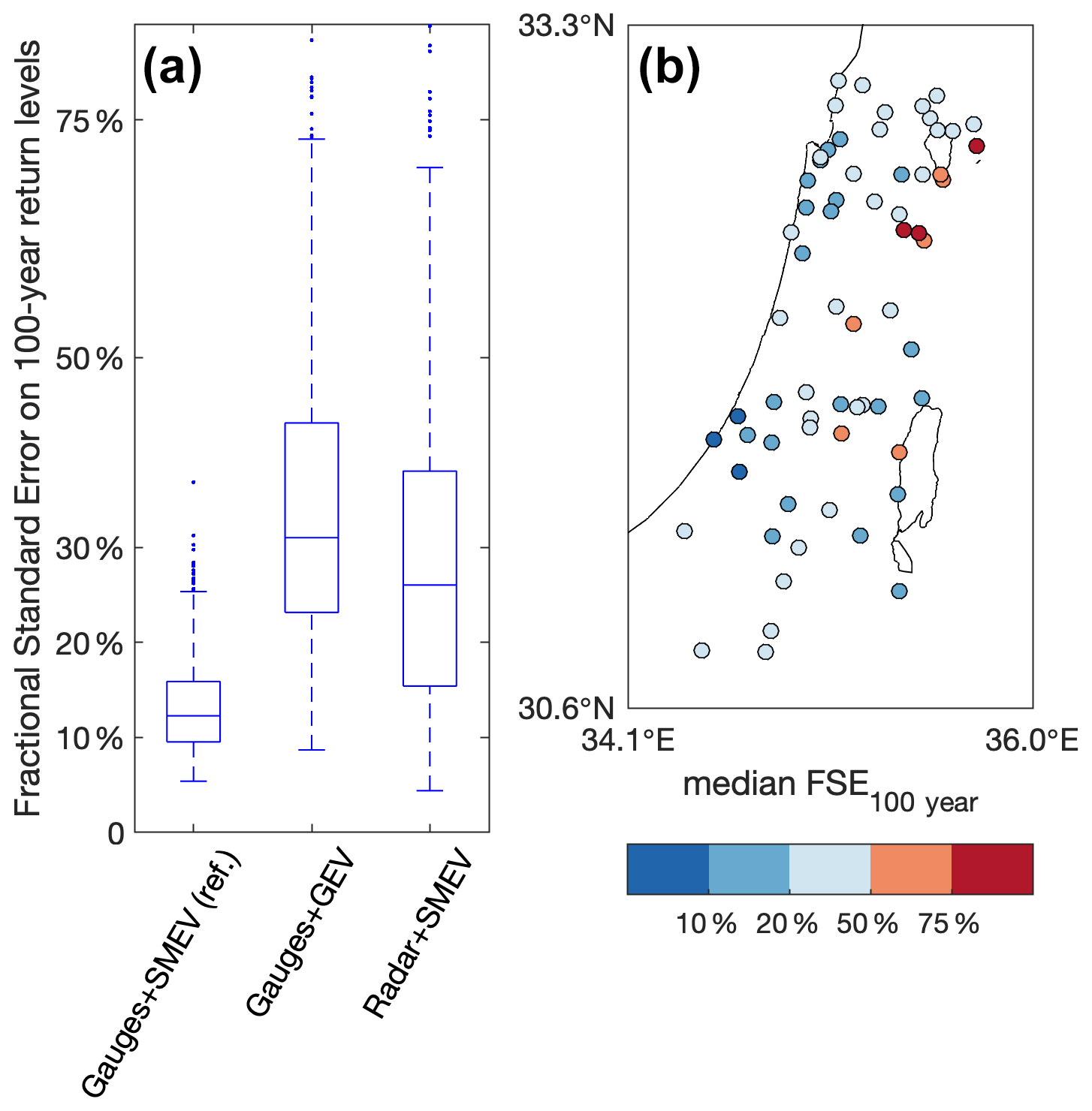
Figure 2Validation of the radar-derived extreme return levels. (a) Fractional standard error (FSE) associated to the estimated 100-year return levels from (i) the reference, i.e. application of SMEV to the gauge full records (gauges + SMEV), (ii) traditional extreme value approaches on the gauge full records (gauges + GEV), and (iii) radar-derived return levels (radar + SMEV); all durations are considered. (b) Spatial distribution of the median (across all durations) FSE for the 100-year return levels estimated using SMEV on the radar archive.
4.2 Coastal effect on design precipitation intensities
The impact of the coastline on extreme precipitation statistics is explored using density plots of the parameters of the intensity distributions (Fig. 3) and of return levels (Fig. 4) as a function of the distance from the coastline (see Fig. 1). Of course, this could not be achieved using rain gauges, since there are no systematic rainfall observations over the sea. Over the Mediterranean Sea (negative distances), the scale parameter tends to be lower and increases while approaching the coast. The offshore dependence of the scale parameter on the distance from the coastline seems rather independent on the duration. In the first 20 km inland, the scale parameter seems to decrease for short durations and to weakly increase for long durations. Since the offshore distance from the coast is somehow correlated to the distance from the radar, and no rain gauges are available over the sea for the adjustment procedure, one could claim that these low offshore values could be caused by radar range effects. To ensure that this is not the case, we compared them with the results from a convection-permitting weather model, which is obviously not impacted by the radar observation geometry. The superimposed red solid lines in Fig. 3a–d show the normalized maximum intensities averaged over 41 heavy precipitation events derived from a convection-permitting Weather Research and Forecasting (WRF) model of a spatial resolution similar to the radar (1 km2; see details in Armon et al., 2020). The weather model shows the same behavior as the radar, confirming that this is indeed a climatic signal.
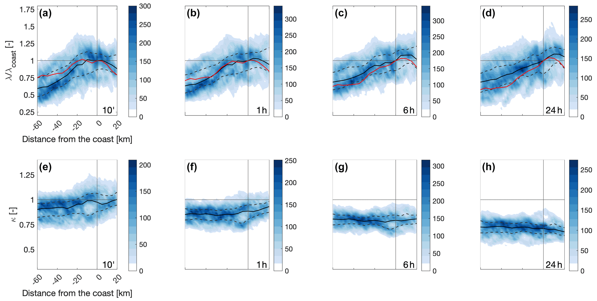
Figure 3Density plots of the scale (a–d) and shape parameters (e–h) as a function of the distance from the coastline (see dashed lines in Fig. 1) for durations of 10 min and 1, 6, and 24 h. Color shading represents the number of radar pixels in bins of 2 km by 0.05 (a–d) and 2 km by 0.01 (e–h). Negative distances represent offshore areas. The median and 25th–75th quantiles of the distribution along 5 km bins are shown as solid black lines and dashed black lines, respectively. In order to have comparable values across durations, scale parameters (a–d) are normalized over the median value at the coast. For comparison, solid red lines show the median of the normalized maximum intensities (which can be considered as a proxy for the scale parameter) from convection-permitting Weather Research and Forecasting (WRF) model simulations of 41 heavy precipitation events in the region (details in Armon et al., 2020). This confirms that the decrease offshore is a climatic signal and not an artifact due to distance from the radar and lack of rain gauges for the adjustment (see Sect. 5).
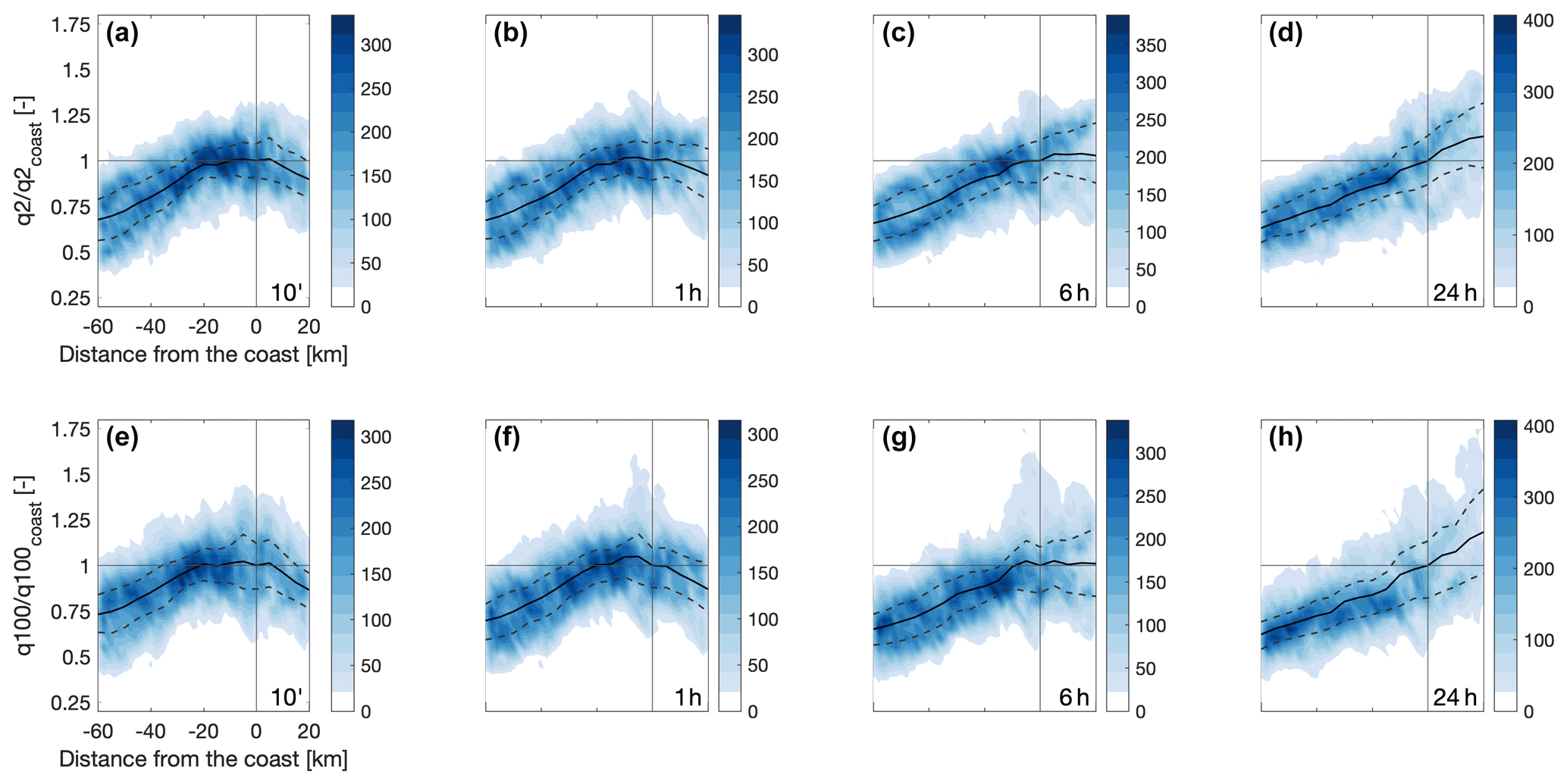
Figure 4Density plots of the 2-year (a–d) and 100-year return levels (e–h) as a function of the distance from the coastline (see dashed lines in Fig. 1) for durations of 10 min and 1, 6, and 24 h. Color shading represents the number of pixels in bins of 2 km by 0.05. Negative distances represent offshore areas. The median and 25th–75th quantiles of the distribution along 5 km bins are shown as solid black lines and dashed black lines, respectively. In order to have comparable values across durations, return levels are normalized over the median value at the coast.
No appreciable variation in the shape parameter as a function of the distance from the coastline is observed offshore (Fig. 3e–h), except a mild increase approaching the coast at short durations and a mild decrease at long durations (both not statistically significant). This implies that no significant change in the heaviness of the intensity distribution tail is observed offshore. In general, the shape parameter offshore is slightly lower than one at 10 min duration (50 % of the pixels have shape values of 0.8–1) and systematically decreases to ∼0.75 at 24 h duration. Inland, the shape tends to increase at short durations (decreasing tail heaviness) and decrease at long durations (increasing tail heaviness). The average yearly number of storms (parameter n), presented in Fig. S2, shows no significant coastal pattern.
Figure 4 shows the dependence of 2-year return levels (which correspond to the median annual maximum value) and 100-year return levels (1 % yearly exceedance probability) on the distance from the coastline. At all durations, low values are observed over the offshore areas in the Mediterranean Sea, which increase towards the coast. As return levels directly respond to the SMEV parameters, and no variations on the shape parameters were found offshore, this is mostly related to the scale parameter patterns highlighted above. Conversely, drastically different effects between short and long durations are observed inland. Extreme return levels of a short duration (up to ∼1 h) tend to peak at or around the coastline, while multi-hour return levels tend to further increase inland, an effect which is more important for more severe return levels. This comes as a response to the combined increase in both the scale parameter and the tail heaviness (Fig. 3).
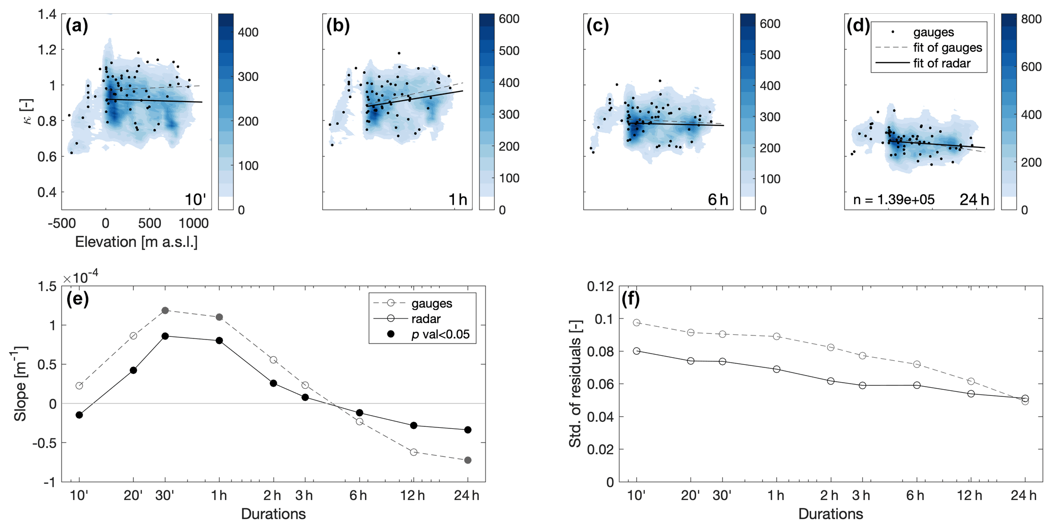
Figure 5(a–d) Density plots of the shape parameter (representing the intensity distribution tail heaviness) as a function of terrain elevation for durations of 10 min and 1, 6, and 24 h. Color shading represents the number of pixels in bins of 50 m by 0.01. Shape parameters estimated from the 10 min rain gauges are shown as black dots. Regression lines computed for all the positive elevations (i.e., excluding the rift valley area depression, which shows a different behavior, and including slopes on both the east and west side of the Judaean Mountains) from weather radar (solid black lines) and 10 min rain gauges (dashed gray lines) are shown. (e) Slope of the shape–elevation regressions computed from weather radar (solid black lines) and gauges (dashed gray lines) as a function of duration. Statistically significant slopes (p<0.05) are displayed with filled circles. Negative slopes imply an increase in tail heaviness with height and vice versa. (f) Standard deviation of the residuals around the regressions for weather radar (solid black lines) and gauges (dashed gray lines) as a function of duration.
4.3 Orographic effect on design precipitation intensities
Orography in the area is weakly related to the distance from the radar, and higher terrain may require the need of higher radar sample volumes to avoid ground echoes and blockages. In particular, due to the lack of rain gauge data and to the high elevation of the radar beam above the second orographic barrier, radar estimates of the scale parameter are here expected to be biased. Therefore, the orographic effect on extreme precipitation statistics is here examined by focusing on the tail heaviness of the intensity distribution (i.e., the shape parameter), which is not expected to be impacted by systematic biases (see also Sect. 4.4). Density plots of the estimated shape parameters as a function of the local terrain elevation are presented in Fig. 5a–d, together with the corresponding estimates based on the rain gauge full records. The quantitative behavior reported by the radar is consistent with the one from the stations, with significant decreases in tail heaviness at short durations (30 min and 1 h) and significant increases at long durations (24 h) (Fig. 5e). In particular, opposing responses emerge at sub-hourly (increasing tail heaviness with elevation), hourly (decreasing), and daily (increasing) timescales. At very short durations (10 min), radar estimates show a statistically significant increase in tail heaviness with elevation (negative slope of the regression in Fig. 5e), while rain gauges show a non-significant decrease. This slight difference can be explained by the fact that no rain gauge is available on the rather large and high-elevation Jordanian plateau (most easterly portion of the radar domain; Fig. 1). The spatially dense radar sampling increases the statistical significance of the derived slopes, allowing an improved appreciation of these relations. Notably, in the rift valley where terrain elevation is below the sea level, the shape parameter increases with elevation at all durations, although achieving a quantification of the effect is difficult here due to the small size of the region and to the small number of available rain gauges.
The spatial variability in the shape parameter also depends on duration for both rain gauges and weather radar, as shown by the residuals from the regression lines (Fig. 5). The standard deviation of the residuals (Fig. 5f) decreases by ∼45 % between 10 min (∼0.09) and 24 h (∼0.05) durations; this decrease seems to be mostly occurring between hourly and daily durations. This implies that larger-scale patterns characterize the statistics of longer-duration extremes, and that larger variability could be related to shorter-duration extremes dominated by convective processes.
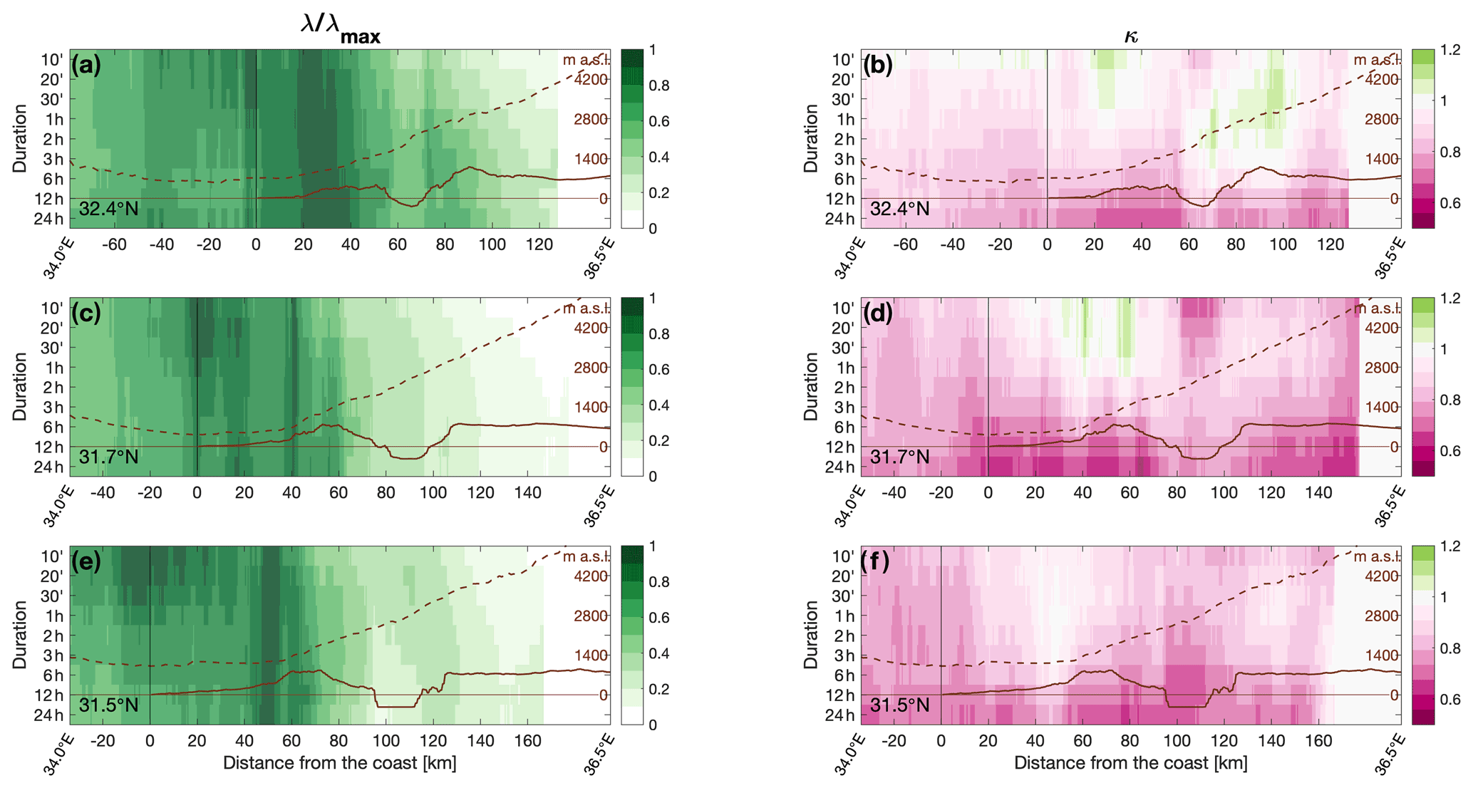
Figure 6Longitudinal variations in the scale (a, c, e) and shape (b, d, f) parameters along the three transects (see Fig. 1) as a function of the distance from the coastline (x axis) and of duration (y axis). Transects are obtained by averaging the 10 km region surrounding the three latitudes. The terrain profile and the sampling height of the lowest non-blocked radar beam are superimposed as solid and dashed lines, respectively (see right hand-side y axis). In order to have comparable values, the scale parameter (a, c, e) at each duration is normalized over the maximum value along longitude.
4.4 Intensity distribution parameters and return levels across longitudinal transects
Longitudinal variations in the intensity distribution parameters (Fig. 6) and of return levels (Fig. 7) are further examined by analyzing the three longitudinal transects characterized from west to east by a sea–land boundary, a mountain range, a major valley, and another mountain range. The location of these transects is chosen based on radar visibility and on the presence of regular orographic profiles. The transects are obtained by averaging the values over a 10 km region surrounding the latitudes (32.4, 31.7, and 31.5∘ N; see Fig. 1). In order to appreciate variations at multiple durations, scale parameter and return levels are normalized, at each duration, over the maximum value along the longitudinal direction. At shorter durations, the scale parameter peaks in the coastal region between few kilometers offshore and 20–30 km inland, and then decreases, roughly in correspondence to the orography (Fig. 6a, c, and e). Conversely, as duration increases, the peak of the scale parameter tends to become wider and to shift inland along the orographic ascent to the first orographic barrier. The rift valley appears as a band with decreased scale parameter, especially at very short and long durations. For hourly and multi-hour durations, the scale parameter seems to increase again around the second orographic barrier (the Jordanian Mountains), although here the high elevation of the radar beam (brown dashed lines) and the absence of 10 min rain gauges to be used for adjusting the radar parameters prevent a good quantitative assessment.
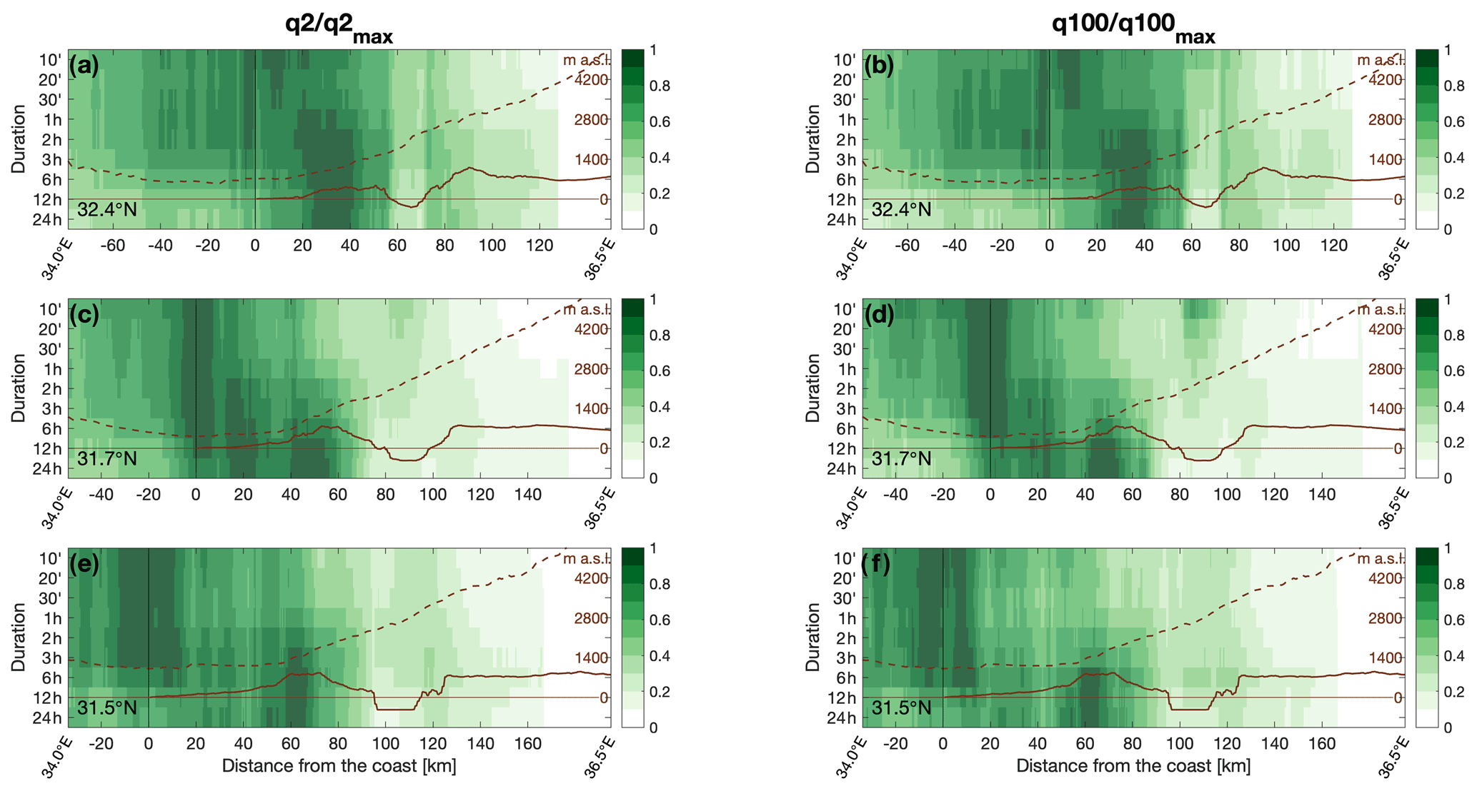
Figure 7Longitudinal variations in the 2- (a, c, e) and 100-year (b, d, f) return levels along the three transects (see Fig. 1) as a function of the distance from the coastline (x axis) and of duration (y axis). Transects are obtained by averaging the 10 km region surrounding the three latitudes. The orographic profile and the sampling height of the lowest non-blocked radar beam are superimposed as solid and dashed lines, respectively (see right-hand side y axis). In order to have comparable values, the return levels at each duration are normalized over the maximum value along longitude.
Overall, the shape parameter tends to decrease with increasing duration, implying an increasing tail heaviness (Fig. 6b, d, and f). More specifically, exponential tails (shape parameters close to 1; white colors) and even lighter tails (higher than 1; green colors) are observed at 10 min durations, while shape parameters as low as 0.6–0.7 (heavy tails; pink colors) are typically observed at 12–24 h durations, especially in the middle transect. Orography seems to induce lighter tails at short durations (≤2 h), with cases of light tails (green colors) corresponding to the first (Judaean Mountains; Fig. 6d) and second (Jordanian plateau; east of the mountaintops; Fig. 6b and f) orographic barriers, although this behavior appears less systematic from the transects alone.
Extreme return levels directly reflect the spatial variability in the parameters (Fig. 7). The 2- and 100-year return levels examined here show qualitatively similar behaviors, although quantitative differences exist due to the variability in the tail heaviness (shape parameter; Fig. 6b, d, and e) and of average yearly number of storms (Fig. S2). At short durations, return levels peak within a ∼20–40 km strip around the coastline. Increasing the duration, the peak gradually moves inland, generally around the first orographic barrier where the largest daily amounts are found. In all cases, the signature of the rift valley depression at hourly and multi-hour durations is clear, with largely decreased values. However, in response to the sharp increase in tail heaviness, 100-year return levels at sub-hourly durations seem to be higher in the rift than in the surrounding areas. This behavior, already reported in previous studies based on traditional methods (Marra and Morin, 2015; Marra et al., 2017), is also found in the 2-year return levels over the central transect, where the sharpest orographic gradient between the Judaean Mountains and the rift valley bottom is found. The impact of the second orographic barrier largely resembles the one of the first orographic barrier (decrease in short-duration return levels; increase of long-duration return levels), although the numbers are smaller here, which is at least partially due to the underestimation of the scale parameter discussed above. This impact is most pronounced over the northern transect, where the Jordanian plateau mountaintops are highest and, in all cases, is evident over the upslope part of the mountains.
The objective of this study is to examine and quantify the relative impacts of coast–land interface and orography on extreme precipitation statistics and design precipitation intensities. While no direct quantification of the return levels is sought here, the proposed method proved skillful in deriving precipitation intensities as high as the once-in-100-years event. Estimates of 100-year return levels obtained by combining 11 years of weather radar data and 10 min rain gauges, using the here-proposed approach, show a median fractional standard error of ∼26 %. This is lower than the fractional standard error of daily amounts in the weather radar archive (Fig. S1). Combining remotely sensed precipitation estimates with rain gauges using the here-proposed framework can, thus, provide spatially distributed estimates of extreme return levels, which are more accurate than the ones obtained using traditional extreme value methods directly on point-scale rain gauge records (median fractional standard error ∼31 %). Nevertheless, given the low methodological uncertainty, the errors in the radar-derived return levels are to be mostly associated to radar errors.
5.1 Coastal and orographic effects on design precipitation intensities
A schematic of the observed coastal and orographic effects on extreme precipitation intensities is presented in Fig. 8. Consistently across the study region, we find an increase in tail heaviness with increasing duration. This was previously reported by Marra et al. (2020, 2021b) and contrasts with previous studies examining the tail of sub-daily intensities (Papalexiou et al., 2018). Nevertheless, as discussed in Marra et al. (2020), the contrast is only apparent and is explained by the different definition of the intensities examined here (ordinary events that are storm maximal intensities) and in previous studies (all non-zero intensities, which come with drastically different number of events at different durations). Exponential tails (shape parameters close to 1; white colors in Fig. 6b, d, and f) and even lighter (higher than 1; green colors) are observed at 10 min durations, while shape parameters as low as 0.6–0.7 (heavy tails; pink colors) are typically observed at 12–24 h durations, especially in the northern transect. These observations agree with the theoretical calculations by Wilson and Tuomi (2005), which, under idealized conditions, predict a stretched exponential distribution with shape parameter equal to two-thirds for extreme storm accumulations (and, therefore, long-duration intensities). An exception to this behavior is the rift valley, which represents a downwind depression to incoming storms from any direction.
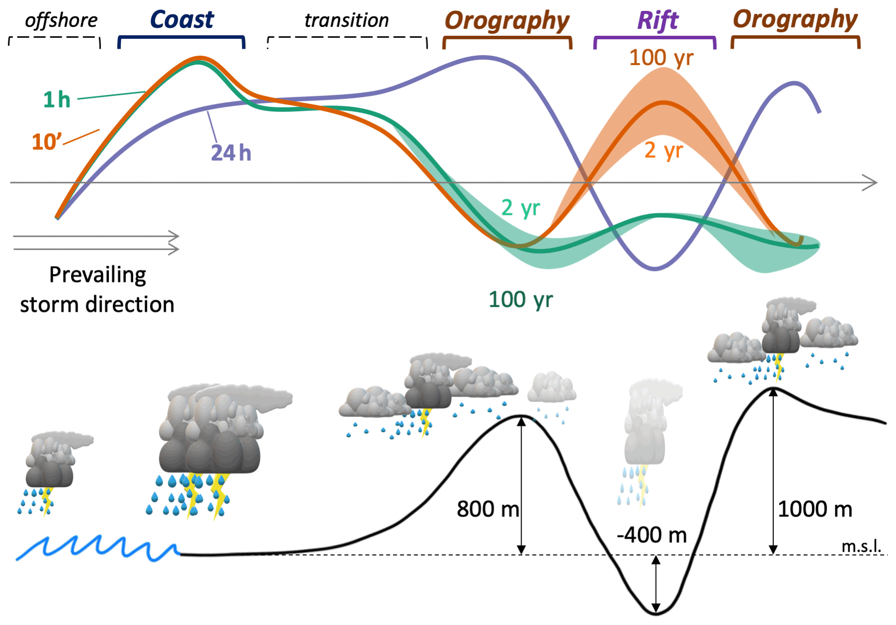
Figure 8Schematic representation of the coastal and orographic effect on extreme precipitation. The qualitative impact of local terrain features (sea–land interface, orographic barriers, and rift valley depression – displayed at the bottom with a black line) on extreme precipitation return levels of 10 min (orange line) and 1 (green) and 24 h (purple) is summarized. The different response of mild (2 year, i.e., 50 % yearly exceedance probability) and extremely severe (100 year, i.e., 1 % yearly exceedance probability) return levels of short duration (10 min, 1 h) to orographic features, which comes as a consequence of the response of the shape parameter of the ordinary events distribution, is displayed using color shades. At the bottom portion of the figure, regions where short-duration convective processes dominate extreme precipitation are indicated with thunderstorms, while regions in which stratiform-like processes and the aggregation of many rain cells dominate extreme precipitation are indicated with thinner precipitating clouds surrounding the thunderstorms. Semi-transparent clouds in the rift indicate that the local occurrence frequency of precipitation events is lower.
Return levels tend to be much smaller offshore than along the coast (median values 60 km offshore are ∼60 %–75 % of the values at the coastline). This comes as a consequence of the decreased scale parameter of the ordinary events distribution. To ensure that this is not related to systematic underestimation due to radar range degradation, we compared it with results from convection-permitting WRF model runs of 41 heavy precipitation events in the area (see Armon et al., 2020), which are obviously not impacted by the radar observation geometry. The weather model (red solid lines in Fig. 3a–d) shows the same behavior as the radar, confirming that this is a climatic signal. Lower offshore return levels, although affected by large noise, were also found using traditional extreme value methods with both radar and satellite observations (Marra et al., 2017).
Short-duration return levels in the region tend to peak in a 20–40 m band around the coastline and in the rift valley, while long-duration return levels tend to peak around orographic barriers. The regime shift occurs between durations of 1–12 h and is more pronounced over the northern portion of the domain (Figs. 6 and 7). In contrast, over the southern portion of the domain, the effect is mostly observed over durations > 6 h, with the coastline exhibiting the largest return levels over durations from 10 min to 6 h (Figs. 6 and 7). In general, opposing responses to orography are observed at sub-hourly (increasing tail heaviness with elevation), hourly (decreasing), and daily (increasing) timescales (Fig. 8). The orographic impact on tail heaviness peaks around hourly durations, as previously reported in Marra et al. (2021b), for the specific case of Mediterranean cyclones. Our results show that this behavior is maintained also when the combined effect of Mediterranean cyclones and other weather systems is considered, although it should be recalled that Mediterranean cyclones account for the majority of storms in most of the examined domain.
5.2 Potential physical mechanisms governing the relation of extreme precipitation with coastline and orography
The shifting of extreme rainfall peak from the coastline towards the mountains with increased duration may be attributed to the different mechanisms involved in the generation of extreme intensity rainfall at different durations. While a detailed meteorological–climatological analysis for the different mechanisms is out of the scope of this paper, there is still a place to mention possible and known causes for these differences. At very short durations, the main driver of high intensity rainfall is instantaneous rain intensity within convective rain cells. This intensity is affected by the amount of moisture in the air and its ascent rate. While moisture for most rain events in the area arrives from the Mediterranean Sea (e.g., Alpert and Shay-El, 1994; Armon et al., 2019) and would cause higher rain rates over the sea, low-level convergence that increases air ascent rates are apparently rather constant over the sea and increase approaching the coastline. This increase is presumably related to the following two main factors: (i) the abrupt increase in drag coefficient at the coast and (ii) the interaction of mesoscale and synoptic winds in the presence of a curved coastline (e.g., Colle et al., 2002). The increase in drag coefficient, caused by larger roughness of the land versus the sea, slows down landward winds and triggers a low-level velocity convergence (e.g., Bergeron, 1949; Roeloffzen et al., 1986; Colle and Yuter, 2007). Neglecting friction, one can commonly think of large-scale atmospheric horizontal wind flows as a balance between the Coriolis, the centrifugal, and the pressure gradient forces. This approximation, called the gradient flow, is violated close to the ground where friction plays a larger role (chap. 4 in Holton, 2004). When increased friction is added upon a balanced gradient flow, such as in the proximity of the coastline, a secondary circulation regime is initiated in which winds in a cyclonic flow tend to flow inward towards the low-level center (chap. 5 in Holton, 2004). This change in wind direction may increase wind curvature and, thus, increase low-level air ascent. Similarly, the interaction of mesoscale winds such as the land–sea breeze with the synoptic wind, especially in the presence of a curved coastline, may enhance instantaneous rain rates because of mesoscale convergence between the two sources of wind (e.g., Neumann, 1951; Andersson and Gustafsson, 1994; Bummer et al., 1995).
Examination of the time of the day at which the highest short-duration intensities (i.e., the ordinary events in the distribution tail, defined here as the largest 45 %) are observed (Fig. 9) shows that the highest offshore intensities tend to occur in the early morning (00:00–06:00 LT – local time) or morning (06:00–12:00 LT), and they shift to mostly morning (06:00–12:00 LT) at the coastline and near inland. This supports the above-proposed mechanism, in which the convergence created by the superposition of the westerly winds typical of Mediterranean cyclones with land breeze, which is expected to peak in the early morning hours when the sea is the warmest compared to the land, could be a contributing factor for the short-duration intensity peak around the coastline. High short-duration intensities in regions where orographic lifting typically dominates (the western side of the Judaean Mountains and the Jordanian plateau) tend to peak in the afternoon (12:00–18:00 LT), suggesting that the diurnal–thermal instability driven by the heating of the ground could here interact with orographic lifting enhancing the convective vertical motions. Conversely, on the lee side of the Judaean Mountains, short-duration intensities seem to peak in the morning hours (06:00–09:00 LT), although this signal is not confirmed by the in situ rain gauges (Fig. 9), which show peaks more concentrated in the early afternoon (12:00–15:00 LT). This mismatch might be caused by the large elevation difference between the radar sampling volumes (here ∼3000 m a.s.l. and above; see profiles in Figs. 5 and 6) and the terrain elevation, where rain gauges measure (even 400 m b.m.s.l.). The radar might systematically overshoot the core of shallow convection, and in addition, the stronger convection captured by the radar might be overestimated due to evaporation of the hydrometeors along their falling path.
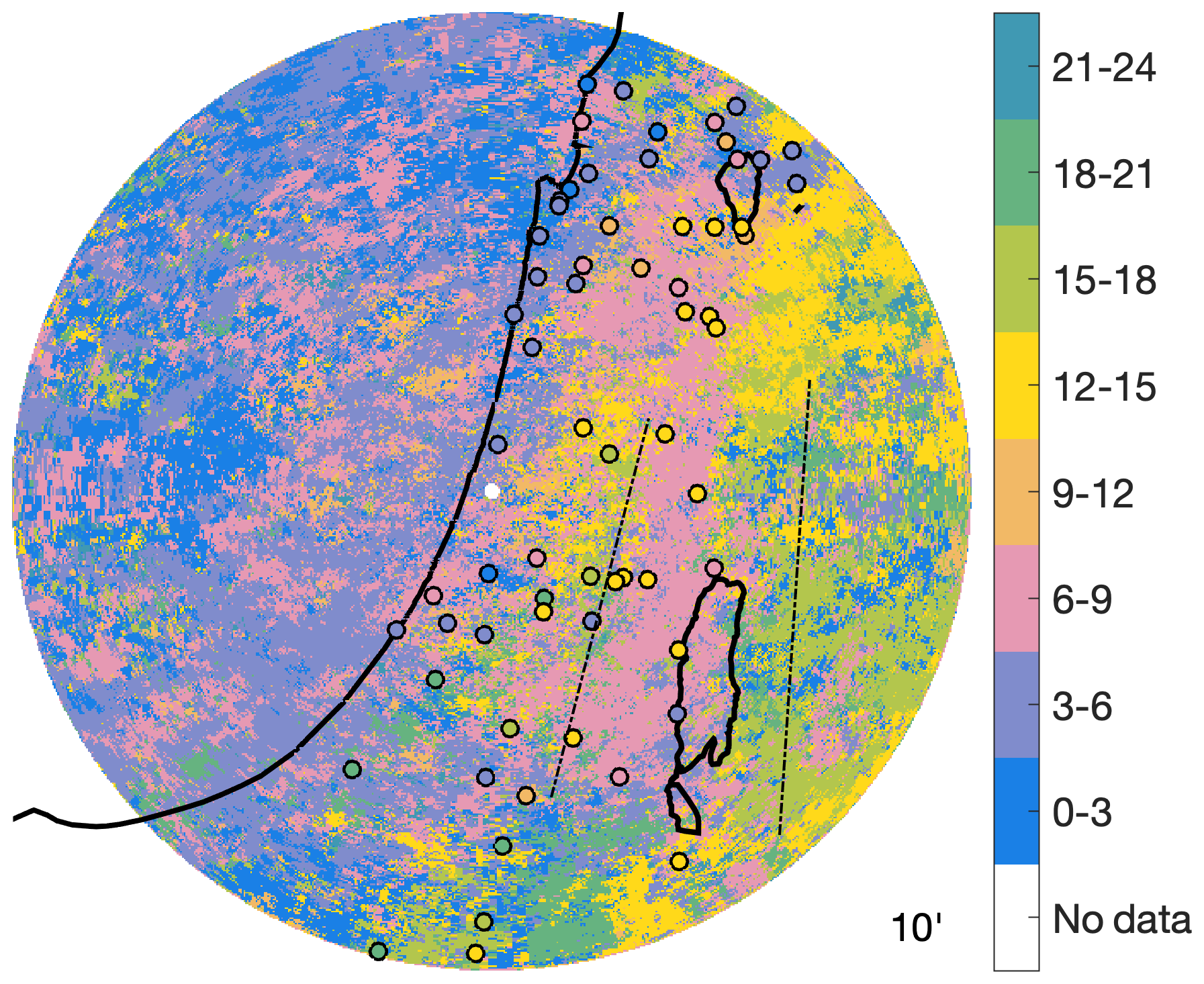
Figure 9Time of the day at which the highest 45 % of the ordinary events (i.e., the storm maximal intensities defining the tail of the intensity distribution) at 10 min duration are typically observed. Circles colored with the same color scheme show the corresponding values obtained from the 10 min rain gauges. Dot–dashed lines show the approximate location of the peaks of the two main orographic barriers.
Farther away from the radar, in both the eastern and southern areas where climate is drier (Fig. 1), short-duration afternoon-to-night peaks are prevailing (north, east, and south of the Dead Sea). This may reflect the higher impact of local thunderstorms which rely on the diurnal heating to bring air ascent to high-enough elevations independent of orography (Sharon and Kutiel, 1986; Dayan et al., 2001, 2021; Armon et al., 2019; Rinat et al., 2021). This might explain the reversed behavior with regions affected by orography and the heavier tails previously observed in these arid areas (Marra et al., 2017; Marra and Morin, 2015).
In contrast to the short-duration rainfall, high multi-hour intensities in the region are mainly a result of the aggregation of multiple rain cells over a specific location and to the shift of extremes towards more stratiform-like processes. They are, thus, less dependent on the instantaneous rain rates and are expected to increase in regions where spatial and temporal rainfall coherence is enhanced. The mountain range causes extreme rain cells to be surrounded by regions with lower-intensity stratiform-like precipitation and to cover a larger area with lower rain rates (Peleg and Morin, 2012; Marra et al, 2021b). Additionally, the orographic lifting tends to squeeze the remaining moisture from the air more efficiently to provide more rainfall in total (Houze et al., 2001; Roe, 2005). Indeed, previous studies in the region found that the area of rain cells is increased inland (Karklinski and Morin, 2006; Peleg and Morin, 2012) and that the temporal autocorrelation of rainfall is larger over the mountains compared to the coastal region (Marra et al., 2021b).
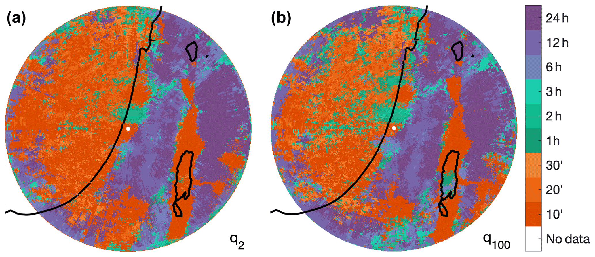
Figure 10Durations at which the local 2- (a) and 100-year (b) return levels are the strongest. At each duration, intensities are ranked among all pixels so as to associate 1 to the largest value over the region and 0 to the smallest. The maps display the duration which, at each pixel, has the largest rank.
Figure 10 presents, for each pixel, the duration at which the relative rank (among all pixels) of its 2- and 100-year return level is the highest. Short-duration (10–20 min) intensities dominate offshore and inland in proximity of the shoreline, over the rift valley, and in the southern portion of the domain, while long durations (6–24 h) dominate in the inland areas, where orography is more pronounced. This pattern resembles the results seen previously (e.g., Fig. 8), highlighting the governing hydrometeorological patterns. Namely, short-duration high-intensity convective processes are the main reason for heavy precipitation close to the coastline where moisture is plentiful, which makes the short-duration events (orange colors) rank first in this region. On the other hand, longer-duration processes require the climbing of air parcels over the mountains (e.g., Alpert, 1986; Roe, 2005), which causes a reorganization of the convective processes (with differential responses at 10 min and 1 h scales) and leads to orographic rainfall with long-lasting stratiform-like processes. This causes mountainous regions to be characterized by long-duration extremes ranking first (purple regions in Fig. 10). Descending from the mountaintops (Figs. 1 and 9), air parcels dry and precipitation is inhibited. In these regions, where conditions are more arid, and along the desert at the southern part of the region, rainfall is spottier and more local (e.g., Sharon and Kutiel, 1986), and its extremes are generally related to rare but sometimes violent convection, which is translated into orange colors in Fig. 10. Similar patterns are also observed on the northern shoreline, where mountain reliefs are close to the coastline, possibly due to the simultaneous impact of coastal and orographic effects.
5.3 Implications for risk management
Roughly 50 % of the population in the region is concentrated in the coastal plains, mainly in cities within 10–20 km from the coastline (CBS, 2016; Bitan and Zviely, 2019). Population growth and migration are expected to disproportionally increase the population density in these coastal cities (Neumann et al., 2015; UN-DESA, 2018). Short-duration precipitation intensities are crucial triggers of pluvial urban flooding, which cause casualties and important losses every year (Cristiano et al., 2017; Villarini et al., 2010). Our results, made possible by the use of distributed rainfall estimates from a weather radar, show that these intensities are stronger in the highly populated coastal areas (orange colors in Fig. 10) of the region, with important implications for urban flood risk management. Moreover, future projections show an increase in the short-duration extreme precipitation intensities in the area (Armon et al., 2022). Given the alarming projections in terms of sea level rise, explicit consideration of the compound impact of extreme rain intensities and storm surges under future scenarios should be specifically addressed in future planning of coastal cities (Zscheischler et al., 2018).
Considering flash flood generation and watershed response, it is interesting to note that short durations (10–20 min; orange colors in Figs. 8 and 10) intensities tend to dominate extremes offshore, over the coastal regions, and in the rift, while longer durations (6–24 h; purple colors in Figs. 8 and 10) tend to dominate extremes inland and over the orographic regions. These spatial patters coincide, in some cases, with the characteristic response time of watersheds. As mentioned above, short-duration extremes can lead to urban flooding over the vast built area near the shore but also in arid watersheds in the rift and in the south of the region (see areas with mean annual rainfall < 200 mm yr−1; Fig. 1), due to the typical fast hydrological response of these areas (e.g., Morin et al., 2001; Zoccatelli et al., 2019). Conversely, watersheds draining inland regions north and west of the Judaean Mountains are typically covered by agricultural areas, forests, or other natural land uses and would typically show a few hours of characteristic timescales (Zoccatelli et al., 2019); for example, the time of the concentration of watersheds with ∼50 km length and ∼600 m height (numbers in the range of the watersheds west of the Judaean Mountains) is ∼3.5 h, based on Johnstone and Cross (1949).
We propose and test a novel methodology for extreme precipitation frequency analysis that allows us to adjust relatively short archives of weather radar precipitation estimates using rain gauges as a reference. The approach is based on the simplified metastatistical extreme value (SMEV) formulation and relies on the adjustment of the remotely sensed information in the SMEV parameter space. The methodology provides spatially distributed, high-resolution statistical descriptions of extremes which accurately reflect the statistics of in situ observational records. Combining 11 years of weather radar data with 10 min rain gauge data in the southeastern Mediterranean, we obtain estimates of 100-year return levels characterized by standard errors of the order of ∼26 %, which is lower than the standard errors obtained using traditional approaches on rain gauge data. We then used the obtained spatially distributed, high-resolution statistical descriptions of extremes to describe and quantify the distinct signature of coastlines and orography on extreme precipitation statistics and design precipitation intensities at multiple sub-daily durations.
The scale parameter of the rain intensity distributions tends to be lower offshore and to increase approaching the coast at all durations (10 min to 24 h). At short and hourly durations, the scale parameter peaks at the coastline, while at longer durations it tends to peak a few kilometers inland, corresponding to the orographic barriers. The distributions tail heaviness is rather uniform above the sea and rapidly changes inland, with opposing directions at short (decreasing tail heaviness) and long (increasing tail heaviness) durations. The orographic impact on the intensity distributions shows a decrease in tail heaviness at short durations, which peaks at hourly durations, and an increase in tail heaviness at long durations; this confirms previous results based on the systematic interaction of Mediterranean cyclones with a regular orographic barrier (Marra et al., 2021b) and suggests this could be a more general behavior not strictly related to the physical processes typical of Mediterranean cyclones in the region. The overall impact results in increasing return levels moving offshore towards the coastline and in opposing behaviors at different durations inland, with decreasing extremes at short and hourly durations and increasing extremes at long durations. Short- and hourly duration return levels tend to peak in proximity of the coastline; long-duration return levels tend to peak inland, corresponding to orographic ascents and mountaintops.
We identify the following three main regimes which respond differently to coastal and orographic forcing: (i) very short durations (∼10 min), mainly related to the peak intensity of convective rain cells (intensity-dominated regime), (ii) hourly durations, related to the rainfall yield (and, thus, to the spatiotemporal organization) of individual convective cells, and (iii) long durations (∼6–24 h), related to the accumulation of multiple convective cells and to long-lasting stratiform processes (Fig. 8). These regimes have also been recently observed in the orographic impact on extreme precipitation in the Alps (Formetta et al., 2022). Convective processes account for higher extremes near the coastline; this is presumably related to increased drag coefficient and to interactions of the synoptic and mesoscale systems, as suggested by the early morning timing of coastal extremes. Conversely, the short-duration extremes in orography-dominated regions tend to peak in the afternoon, suggesting a contribution from the diurnal thermal instability. Long-duration extremes are higher in regions where spatial and temporal rainfall coherence is enhanced, such as orographic regions, where orographic lifting smooths the precipitation field. The distinct coastal and orographic effects at different durations are expected to modulate the temporal scales of the most relevant local impacts, i.e., short-scale hazards (e.g., urban floods, debris flows) are more of concern for the coastal and rift regions, while longer-scale hazards (e.g., flash floods) could be more relevant over mountainous areas.
Given the relatively flexible requirements in terms of availability and record length of weather radar and rain gauge data, the here-presented methodology is deemed suitable for extreme multi-duration precipitation frequency analyses in many other regions worldwide. Specifically, it could help by (i) improving the quantification of local return levels without the need for homogeneity and/or temporal scaling assumptions and (ii) increasing the understanding of the local climatology of extreme multi-duration precipitation. In addition, (iii) it could be combined with information from climate models and local constraints to derive observationally sound projections of future extreme return levels for climate change impact studies.
Codes used for the estimation of SMEV and GEV parameters and return levels are freely available at https://doi.org/10.5281/zenodo.3971558 (Marra, 2020).
Rain gauge data were provided and preprocessed by the Israel Meteorological Service and are freely available at https://ims.data.gov.il/ (last access: 13 March 2022) (Hebrew only). Original weather radar data were provided by the Israel Meteorological Service (https://ims.gov.il/en, last access: 13 March 2022). Corrected and gauge-adjusted radar data are available upon request to the head of the Hydrometeorology lab at the Hebrew University of Jerusalem, Efrat Morin (efrat.morin@mail.huji.ac.il).
The supplement related to this article is available online at: https://doi.org/10.5194/hess-26-1439-2022-supplement.
FM conceptualized the paper with MA and EM, conducted the analysis and curated the data with MA, wrote the paper, and participated in the review and editing process with MA and EM.
The contact author has declared that neither they nor their co-author has any competing interests.
Publisher's note: Copernicus Publications remains neutral with regard to jurisdictional claims in published maps and institutional affiliations.
This paper collects years of efforts. Many of the methods used to create the weather radar archive were developed by the team in the past years, in addition to the novel statistical methodology used for extreme value analyses. Similarly, studies about extreme precipitation in the region and about the use of remotely sensed datasets for precipitation frequency analyses were published by the team. The number of self-citations is, thus, large. We did our best not to inflate it, and we hope the text will clarify why these citations are needed.
This study is a contribution to the HyMeX program, and is based upon work from COST Action CA19109 “MedCyclones” supported by COST – European Cooperation in Science and Technology. Francesco Marra thanks the Institute of Atmospheric Sciences and Climate (ISAC) of the National Research Council of Italy (CNR) for the support. Moshe Armon was supported by an ETH Zurich Postdoctoral Fellowship (project no. 21-1 FEL-67), by the Stiftung fuer naturwissenschaftliche und technische Forschung, and the ETH Zurich Foundation. The authors thank Uri Dayan, for the fruitful discussions, and the two reviewers, for the constructive comments.
This research has been supported by the Israel Science Foundation (grant no. 1069/18).
This paper was edited by Yue-Ping Xu and reviewed by Lihua Xiong and Gaby Gründemann.
Allamano, P., Claps, P., Laio, F., and Thea, C.: A data-based assessment of the dependence of short-duration precipitation on elevation, Phys. Chem. Earth, 34, 635–641, https://doi.org/10.1016/j.pce.2009.01.001, 2009.
Alpert, P.: Mesoscale indexing of the distribution of orographic precipitation over high mountains, J. Clim. Appl. Meteorol., 25, 532–545, https://doi.org/10.1175/1520-0450(1986)025<0532:MIOTDO>2.0.CO;2, 1986.
Alpert, P. and Shafir, H.: Meso c-scale distribution of orographic precipitation: numerical study and comparison with precipitation derived from radar measurements, J. Appl. Meteorol., 28, 1105–1117, https://doi.org/10.1175/1520-0450(1989)028<1105:MSDOOP>2.0.CO;2, 1989.
Alpert, P. and Shay-El, Y.: The moisture source for the winter cyclones in the EM, Israel Meteorological Research Papers 5, 20–27, available at https://www.researchgate.net/profile/Pinhas-Alpert/publication/283745573_The_moisture_source_for_the, (last access: 13 March 2022), 1994.
Alpert, P., Osetinsky, I., Ziv, B., and Shafir, H.: Semi-objective classification for daily synoptic systems: Application to the eastern Mediterranean climate change, Int. J. Climatol., 24, 1001–1011, https://doi.org/10.1002/joc.1036, 2004.
Amponsah, W., Ayral, P. A., Boudevillain, B., Bouvier, C., Braud, I., Brunet, P., Delrieu, G., Didon-Lescot, J. F., Gaume, E., Lebouc, L., Marchi, L., Marra, M., Morin, E., Nord, G., Payastre, O., Zoccatelli, D., and Borga, M.: Integrated high-resolution dataset of high intensity European and Mediterranean flash floods, Earth Syst. Sci. Data, 10, 1783–1794, https://doi.org/10.5194/essd-10-1783-2018, 2018.
Andersson, T. and Gustafsson, N.: Coast of departure and coast of arrival: two important concepts for the formation and structure of convective snowbands over seas and lakes, Mon. Weather Rev., 122, 1036–1049, https://doi.org/10.1175/1520-0493(1994)122<1036:CODACO>2.0.CO;2, 1994.
Andrieu, H., Creutin, J. D., Delrieu, G., and Faure, D.: Use of a weather radar for the hydrology of a mountainous area. Part I: radar measurement interpretation, J. Hydrol., 193, 1–25, https://doi.org/10.1016/S0022-1694(96)03202-7, 1997.
Armon, M., Dente, E., Smith, J. A., Enzel, Y., and Morin, E.: Synoptic-scale control over modern rainfall and flood patterns in the levant drylands with implications for past climates, J. Hydrometeorol., 19, 1077–1096, https://doi.org/10.1175/JHM-D-18-0013.s1, 2018.
Armon, M., Morin, E., and Enzel, Y.: Overview of modern atmospheric patterns controlling rainfall and floods into the Dead Sea: Implications for the lake's sedimentology and paleohydrology, Quaternary Sci. Rev., 216, 58–73, https://doi.org/10.1016/j.quascirev.2019.06.005, 2019.
Armon, M., Marra, F., Enzel, Y., Rostkier-Edelstein, D., and Morin, E.: Radar-based characterisation of heavy precipitation in the eastern Mediterranean and its representation in a convection-permitting model, Hydrol. Earth Syst. Sci., 24, 1227–1249, https://doi.org/10.5194/hess-24-1227-2020, 2020.
Armon, M., Marra, F., Garfinkel, C., Rostkier-Edelstein, D., Adam, O., Dayan, U., Enzel, Y., and Morin, E.: Reduced rainfall in future heavy precipitation events related to contracted rain area despite increased rain rate, Earth's Future, 9, e2021EF002397, https://doi.org/10.1029/2021EF002397, 2022.
Arnbjerg-Nielsen, K., Willems, P., Olsson, J., Beecham, S., Pathirana, A., Gregersen, I. B., Madsen, H., and Nguyen, V. T. V.: Impacts of climate change on rainfall extremes and urban drainage systems: a review, Water Sci. Technol., 68, 16–28, https://doi.org/10.2166/wst.2013.251, 2013.
Attema, J. J. and Lenderink, G.: The influence of the North Sea on coastal precipitation in the Netherlands in the present-day and future climate, Clim. Dynam., 42, 505–519, https://doi.org/10.1007/s00382-013-1665-4, 2014.
Avanzi, F., De Michele, C., Gabriele, S., Ghezzi, A., and Rosso, R.: Orographic Signature on Extreme Precipitation of Short Durations, J. Hydrometeorol., 16, 278–294, https://doi.org/10.1175/JHM-D-14-0063.1, 2015.
Belachsen, I., Marra, F., Peleg, N., and Morin, E.: Convective rainfall in a dry climate: Relations with synoptic systems and flash-flood generation in the Dead Sea region, Hydrol. Earth Syst. Sci., 21, 5165–5180, https://doi.org/10.5194/hess-21-5165-2017, 2017.
Bergeron, T.: The Problem of Artificial Control of Rainfall on the Globe1: II. The Coastal Orographic Maxima of Precipitation in Autumn and Winter, Tellus, 1, 15–32, https://doi.org/10.1111/j.2153-3490.1949.tb01264.x, 1949.
Bevacqua, E., Maraun, D., Vousdoukas, M. I., Voukouvalas, M. I., Mentaschi, L., and Widmann, M.: Higher probability of compound flooding from precipitation and storm surge in Europe under anthropogenic climate change, Sci. Adv., 5, 9, https://doi.org/10.1126/sciadv.aaw5531, 2019.
Bitan, M. and Zviely, D.: Lost value assessment of bathing beaches due to sea level rise: a case study of the Mediterranean coast of Israel, J. Coast. Conserv., 23, 773–783, https://doi.org/10.1007/s11852-018-0660-7, 2019.
Blöschl, G., Bierkens, M. F. P., Chambel, A., et al.: Twenty-three unsolved problems in hydrology (UPH) – a community perspective, Hydrolog. Sci. J, 64, 1141–1158, https://doi.org/10.1080/02626667.2019.1620507, 2019.
Buishand, T. A.: Extreme rainfall estimation by combining data from several sites, Hydrolog. Sci. J., 36, 345–365, https://doi.org/10.1080/02626669109492519, 1991.
Bummer, B., Hennemuth, B., Rhodin, A., and Thiemann, S.: Interaction of a cold front with a sea-breeze front Observations, Tellus A, 47, 383–402, https://doi.org/10.1034/j.1600-0870.1995.t01-2-00001.x, 1995.
Burlando, P. and Rosso, R.: Scaling and multiscaling models of depth-duration-frequency curves for storm precipitation, J. Hydrol., 187, 45–64, https://doi.org/10.1016/S0022-1694(96)03086-7, 1996.
CBS – Central Bureau of Statistics: Population and demography, State of Israel, http://www.cbs.gov.il/reader/shnaton/shmapheb_new.htm?CYear=2010&Vol=61&CSubject=30 (last access: 8 June 2021), 2016.
Chow, V. T., Maidment, D. R., and Mays, L. W.: Applied Hydrology, McGraw-Hill, ISBN 0-07-010810-2, 1988.
Colle, B. A. and Yuter, S. E.: The Impact of Coastal Boundaries and Small Hills on the Precipitation Distribution across Southern Connecticut and Long Island, New York, Mon. Weather Rev., 135, 933–954, https://doi.org/10.1175/MWR3320.1, 2007.
Colle, B. A., Smull, B. F., and Yang, M. J.: Numerical simulations of a landfalling cold front observed during COAST: Rapid evolution and responsible mechanisms, Mon. Weather Rev., 130, 1945–1966, https://doi.org/10.1175/1520-0493(2002)130<1945:NSOALC>2.0.CO;2, 2002.
Collier, C. G.: Applications of Weather Radar Systems: A Guide to Uses of Radar Data in Meteorology and Hydrology, Wiley, West Sussex, UK, ISBN 0471960136, 1989.
Courty, L. G., Wilby, R. L., Hillier J. K., and Slater, L.: Intensity-duration-frequency curves at the global scale, Environ. Res. Lett., 14, 084045, https://doi.org/10.1088/1748-9326/ab370a, 2019.
Cristiano, E., ten Veldhius, M.-.C., and van de Giesen, N.: Spatial and temporal variability of rainfall and their effects on hydrological response in urban areas – a review, Hydrol. Earth Syst. Sci., 21, 3859–3878, https://doi.org/10.5194/hess-21-3859-2017, 2017.
Dayan, U., Ziv, B., Margalit, A., Morin, E., and Sharon, D.: A severe autumn storm over the middle-east: synoptic and mesoscale convection analysis, Theor. Appl. Climatol., 69, 103–122, https://doi.org/10.1007/s007040170038, 2001.
Dayan, U., Lensky, I. M., Ziv, B., and Khain, P.: Atmospheric conditions leading to an exceptional fatal flash flood in the Negev Desert, Israel, Nat. Hazards Earth Syst. Sci., 21, 1583–1597, https://doi.org/10.5194/nhess-21-1583-2021, 2021.
Delrieu, G., Andrieu, H., and Creutin, J. D.: Quantification of path-integrated attenuation for X and C-band weather radar systems operating in Mediterranean heavy rainfall, J. Appl. Meteorol., 39, 840–850, https://doi.org/10.1175/1520-0450(2000)039<0840:QOPIAF>2.0.CO;2, 2000.
Demirdjian, L., Zhou, Y., and Huffman, G.: Statistical modelling of extreme precipitation with TRMM data, J. Appl. Meteorol. Clim., 57, 15–30, https://doi.org/10.1175/JAMC-D-17-0023.1, 2018.
de Vries, A.J., Tyrlis, E., Edry, D., Krichak, S. O., Steil, B., and Lelieveld, J.: Extreme precipitation events in the Middle East: dynamics of the Active Red Sea Trough, J. Geophys. Res.-Atmos. 118, 7087–7108, https://doi.org/10.1002/jgrd.50569, 2013.
Eldardiry, H., Habib, E., and Zhang, Y.: On the Use of Radar-Based Quantitative Precipitation Estimates for Precipitation Frequency Analysis, J. Hydrol., 531, 441–453, https://doi.org/10.1016/j.jhydrol.2015.05.016, 2015.
Enzel, Y., Bookman, R., Sharon, D., Gvirtzman, H., Dayan, U., Ziv, B., and Stein, M.: Late Holocene climates of the Near East deduced from Dead Sea level variations and modern regional winter rainfall, Quatern. Res., 60, 263–273, https://doi.org/10.1016/j.yqres.2003.07.011, 2003.
Formetta, G., Marra, F., Dallan, E., Zaramella, M., and Borga, M.: Differential orographic impact on sub-hourly, hourly, and daily extreme precipitation, Adv. Water Resour., 149, 104085, https://doi.org/10.1016/j.advwatres.2021.104085, 2022.
Forzieri, G., Pecchi, M., Girardello, M., Mauri, A., Klaus, M., Nikolov, C., Rüetschi, M., Gardiner, B., Tomaštík, J., Small, D., Nistor, C., Jonikavicius, D., Spinoni, J., Feyen, L., Giannetti, F., Comino, R., Wolynski, A., Pirotti, F., Maistrelli, F., Savulescu, I., Wurpillot-Lucas, S., Karlsson, S., Zieba-Kulawik, K., Strejczek-Jazwinska, P., Mokroš, M., Franz, S., Krejci, L., Haidu, I., Nilsson, M., Wezyk, P., Catani, F., Chen, Y.-Y., Luyssaert, S., Chirici, G., Cescatti, A., and Beck, P. S. A.: A spatially explicit database of wind disturbances in European forests over the period 2000–2018, Earth Syst. Sci. Data, 12, 257–276, https://doi.org/10.5194/essd-12-257-2020, 2020.
Goldreich, Y.: The spatial distribution of annual rainfall in Israel – a review, Theor. Appl. Climatol., 50, 45–59, https://doi.org/10.1007/BF00864902, 1994.
Goudenhoofdt, E., Delobbe, L., and Willems, P.: Regional frequency analysis of extreme rainfall in Belgium based on radar estimates, Hydrol. Earth Syst. Sci., 21, 5385–5399, https://doi.org/10.5194/hess-21-5385-2017, 2017.
Haiden, T., Kerschbaum, M., Kahlig, P., and Nobilis, F.: A refined model of the influence of orography on the mesoscale distribution of extreme precipitation, Hydrolog. Sci. J., 37, 417–427, https://doi.org/10.1080/02626669209492609, 1992.
Heiblum, R. H., Koren, I., and Altaratz, O.: Analyzing coastal precipitation using TRMM observations, Atmos. Chem. Phys., 11, 13201–13217, https://doi.org/10.5194/acp-11-13201-2011, 2011.
Hicks, N. S., Smith, J. A., Miller, A. J., and Nelson, P. A.: Catastrophic flooding from an orographic thunderstorm in the central Appalachians, Water Resour. Res., 41, W12428, https://doi.org/10.1029/2005WR004129, 2005.
Hitschfeld, W. and Bordan, J.: Errors inherent in the radar measurement of rainfall at attenuation wavelengths, J. Meteorol., 11, 5867, https://doi.org/10.1175/1520-0469(1954)011<0058:EIITRM>2.0.CO;2, 1954.
Hochman, A., Harpaz, T., Saaronia, H., and Alpert, P.: Synoptic classification in 21st century CMIP5 predictions over the Eastern Mediterranean with focus on cyclones, Int. J. Climatol., 38, 1476–1483, https://doi.org/10.1002/joc.5260, 2018.
Holton, J. R.: An introduction to Dynamic Meteorology, Chapter 5.4, Elsevier, https://doi.org/10.1017/CBO9781107415324.004, 2004.
Hosking, J. R. M.: L-moments: Analysis and estimation of distributions using linear combinations of order statistics, J. Roy. Stat. Soc. B, 52, 105–124, 1990.
Houze Jr., R. A., James, C. N., and Medina, S.: Radar observations of precipitation and airflow on the Mediterranean side of the Alps: Autumn 1998 and 1999, Q. J. Roy. Meteorol. Soc., 127, 2537–2558, https://doi.org/10.1002/qj.49712757804, 2001.
Hu, L., Nikolopoulos, E. I., Marra, F., Morin, E., Marani, M., and Anagnostou, E. N.: Evaluation of MEVD-based precipitation frequency analyses from quasi-global precipitation datasets against dense rain gauge networks, J. Hydrol., 590, 12564, https://doi.org/10.1016/j.jhydrol.2020.125564, 2020.
Jacobi, S., Bronstert, A., and Heistermann, M.: Rain rate retrieval of partially blocked beams from single-polarized weather radar data, ERAD2014, 218, available at: https://www.researchgate.net/publication/309737854_Rain_rate_retrieval_of_partially_blocked_beams_from_single-polarized_weather_radar_data (last access: 13 March 2022), 2014.
Johnstone, D. and Cross, W. P.: Elements of Applied Hydrology, Ronald Press, New York, ISBN 13: 9781124128436, ISBN 10: 1124128433, 1949.
Karklinsky, M. and Morin, E.: Spatial characteristics of radar-derived convective rain cells over southern Israel, Meteorol. Z., 15, 513–520, https://doi.org/10.1127/0941-2948/2006/0153, 2006.
Katz, R. W., Parlange, M. B., and Naveau, P.: Statistics of extremes in hydrology, Adv. Water Resour., 25, 1287–1304, https://doi.org/10.1016/S0309-1708(02)00056-8, 2002.
Kidd, C., Becker, A., Huffman, G. J., Muller, C. L., Joe, P., Skofronick-Jackson, G., and Kirschbaum, D.: So, how much of the Earth’s surface is covered by rain gauges?, B. Am. Meteorol. Soc., 98, 69–78, https://doi.org/10.1175/BAMS-D-14-00283.1, 2017.
Kleindorfer, P. and Kunreuther, H.: Challenges facing the insurance industry in managing catastrophic risks, in: The Financing of Catastrophe Risk, edtied by: Froot, K. A., University of Chicago Press, ISBN 0-226-26623-0, 1999.
Koutsoyiannis, D., Kozonis, D., and Manetas, A.: A mathematical framework for studying rainfall intensity-duration-frequency relationships, J. Hydrol., 206, 118–135, https://doi.org/10.1016/S0022-1694(98)00097-3, 1998.
Kushnir, Y., Dayan, U., Ziv, B., Morin, E., and Enzel, Y.: Climate of the Levant: Phenomena and mechanisms, in: Quaternary of the Levant: Environments, Climate Change, and Humans, edited by: Enzel, Y. and Ofer, B.-Y., Cambridge University Press, 31–44, https://doi.org/10.1017/9781316106754, 2017.
Lengfeld, K., Kirstetter, P.-E., Fowler, H. J., Yu, J., Becker, A., Flamig, Z., and Gourley, J. J.: Use of radar data for characterizing extreme precipitation at fine scales and short durations, Environ. Res. Lett., 15, 085003, https://doi.org/10.1088/1748-9326/ab98b4, 2020.
Li, Y. and Carbone, R. E.: Offshore propagation of coastal precipitation. J. Atmos. Sci., 72, 4553–4568, https://doi.org/10.1175/JAS-D-15-0104.1, 2015.
Mapes, B. E., Warner, T. T., Xu, M., and Negri, A. J.: Diurnal patterns of rainfall in northwestern South America. Part I: Observations and context, Mon. Weather Rev., 131, 799–812, 2003.
Marani, M. and Ignaccolo, M.: A metastatistical approach to rainfall extremes, Adv. Water Resour., 79, 121–126, https://doi.org/10.1016/j.advwatres.2015.03.001, 2015.
Marchi, L., Cavalli, M., Sangati, M., and Borga, M.: Hydrometeorological controls and erosive response of an extreme alpine debris flow, Hydrol. Process., 23, 2714–2727, https://doi.org/10.1002/hyp.7362, 2009.
Marra, F.: A Unified Framework for Extreme Sub-daily Precipitation Frequency Analyses based on Ordinary Events – data & codes (Version v1), Zenodo [code], https://doi.org/10.5281/zenodo.3971558, 2020.
Marra, F. and Morin, E.: Use of radar QPE for the derivation of Intensity–Duration–Frequency curves in a range of climatic regimes, J. Hydrol., 531, 427–440, https://doi.org/10.1016/j.jhydrol.2015.08.064, 2015.
Marra, F. and Morin, E.: Autocorrelation structure of convective rainfall in semiarid-arid climate derived from high-resolution X-Band radar estimates, Atmos. Res., 200, 126–138, https://doi.org/10.1016/j.atmosres.2017.09.020, 2018.
Marra, F., Nikolopoulos, E. I., Creutin, J. D., and Borga, M.: Radar rainfall estimation for the identification of debris-flow occurrence thresholds, J. Hydrol., 519, 1607–1619, https://doi.org/10.1016/j.jhydrol.2014.09.039, 2014.
Marra, F., Morin, E., Peleg, N., Mei, Y., and Anagnostou, E. N.: Intensity–duration–frequency curves from remote sensing rainfall estimates: comparing satellite and weather radar over the eastern Mediterranean, Hydrol. Earth Syst. Sci., 21, 2389–2404, https://doi.org/10.5194/hess-21-2389-2017, 2017.
Marra, F., Nikolopoulos, E. I., Anagnostou, E. N., and Morin, E.: Metastatistical Extreme Value analysis of hourly rainfall from short records: estimation of high quantiles and impact of measurement errors, Adv. Water Resour., 117, 27–39, https://doi.org/10.1016/j.advwatres.2018.05.001, 2018.
Marra, F., Nikolopoulos, E. I., Anagnostou, E. N., Bárdossy, A., and Morin, E.: Precipitation frequency analysis from remotely sensed datasets: A focused review, J. Hydrol., 574, 699–705, https://doi.org/10.1016/j.jhydrol.2019.04.081, 2019a.
Marra, F., Zoccatelli, D., Armon, M., and Morin, E.: A simplified MEV formulation to model extremes emerging from multiple nonstationary underlying processes, Adv. Water Resour., 127, 280–290, https://doi.org/10.1016/j.advwatres.2019.04.002, 2019b.
Marra, F., Borga, M., and Morin, E.: A unified framework for extreme sub-daily precipitation frequency analyses based on ordinary events, Geophys. Res. Lett., 47, e2020GL090209, https://doi.org/10.1029/2020GL090209, 2020.
Marra, F., Armon, M., Adam, O., Zoccatelli, D., Gazal, O., Garfinkel, C. I., Rostkier-Edelstein, D., Dayan, U., Enzel, Y., and Morin, E.: Towards narrowing uncertainty in future projections of local extreme precipitation, Geophys. Res. Lett., 48, e2020GL091823, https://doi.org/10.1029/2020GL091823, 2021a.
Marra, F., Armon, M., Borga, M., and Morin, E.: Orographic effect on extreme precipitation statistics peaks at hourly time scales, Geophys. Res. Lett., 48, e2020GL091498, https://doi.org/10.1029/2020GL091498, 2021b.
McGraw, D., Nikolopoulos, E. I., Marra, F., and Anagnostou, E. N.: Precipitation frequency analyses based on radar estimates: An evaluation over the contiguous United States, J. Hydrol., 573, 299–310, https://doi.org/10.1016/j.jhydrol.2019.03.032, 2019.
Mekonnen, K., Melesse, A. M., and Woldesenbet, T. A.: Effect of temporal sampling mismatches between satellite rainfall estimates and rain gauge observations on modelling extreme rainfall in the Upper Awash Basin, Ethiopia, J. Hydrol., 598, 126467, https://doi.org/10.1016/j.jhydrol.2021.126467, 2021.
Minder, J. R., Letcher, T. W., Campbell, L. S., Veals, P. G., and Steenburgh, W. J.: The Evolution of Lake-Effect Convection during Landfall and Orographic Uplift as Observed by Profiling Radars, Mon. Weather Rev., 143, 4422–4442, https://doi.org/10.1175/MWR-D-15-0117.1, 2015.
Miniussi, A. and Marra, F.: Estimation of extreme daily precipitation return levels at-site and in ungauged locations using the simplified MEV approach, J. Hydrol., 603, 126946, https://doi.org/10.1016/j.jhydrol.2021.126946, 2021.
Morin, E. and Gabella, M.: Radar-based quantitative precipitation estimation over Mediterranean and dry climate regimes, J. Geophys. Res., 112, D20108, https://doi.org/10.1029/2006JD008206, 2007.
Morin, E., Enzel, Y., Shamir, U., and Garti, R.: The characteristic time scale for basin hydrological response using radar data, J. Hydrol., 252, 1–4, https://doi.org/10.1016/S0022-1694(01)00451-6, 2001.
Neumann, J.: Land breezes and nocturnal thunderstorms, J. Atmos. Sci., 8, 60–67, 1951.
Neumann, B., Vafeidis, A. T., Zimmermann, J., and Nicholls, R. J.: Future Coastal Population Growth and Exposure to Sea-Level Rise and Coastal Flooding – A Global Assessment, PLOS ONE, 10, e0118571, https://doi.org/10.1371/journal.pone.0118571, 2015.
Niziol, T. A., Snyder, W. R., and Waldstreicher, J. S.: Winter weather forecasting throughout the Eastern United States. Part IV: Lake effect snow, Weather Forecast., 10, 61–77, https://doi.org/10.1175/1520-0434(1995)010<0061:WWFTTE>2.0.CO;2, 1995.
Overeem, A., Buishand, T. A., and Holleman, I.: Extreme rainfall analysis and estimation of depth-duration-frequency curves using weather radar, Water Resour. Res., 45, 1–15, https://doi.org/10.1029/2009WR007869, 2009.
Panziera, L., Gabella, M., Zanini, S., Hering, A., Germann, U., and Berne, A.: A radar-based regional extreme rainfall analysis to derive the thresholds for a novel automatic alert system in Switzerland, Hydrol. Earth Syst. Sci., 20, 2317–2332, https://doi.org/10.5194/hess-20-2317-2016, 2016.
Papalexiou, S. M., AghaKouchak, A., and Foufoula‐Georgiou, E.: A diagnostic framework for understanding climatology of tails of hourly precipitation extremes in the United States, Water Resour. Res., 54, 6725–6738, https://doi.org/10.1029/2018WR022732, 2018.
Paranunzio, R., Chiarle, M., Laio, F., Nigrelli, G., Turconi, L., and Luino, F.: New insights in the relation between climate and slope failures at high-elevation sites, Theor. Appl. Climatol., 137, 1765–1784, https://doi.org/10.1007/s00704-018-2673-4, 2019.
Peleg, N. and Morin, E.: Convective rain cells: Radar-derived spatiotemporal characteristics and synoptic patterns over the eastern Mediterranean, J. Geophys. Res., 117, D15116, https://doi.org/10.1029/2011JD017353, 2012.
Peleg, N., Ben-Asher, M., and Morin, E.: Radar subpixel-scale rainfall variability and uncertainty: lessons learned from observations of a dense rain-gauge network, Hydrol. Earth Syst. Sci., 17, 2195–2208, https://doi.org/10.5194/hess-17-2195-2013, 2013.
Peleg, N., Marra, F., Fatichi, S., Paschalis, A., Molnar, P., and Burlando, P.: Spatial variability of rainfall at radar subpixel scale, J. Hydrol., 556, 922–933, https://doi.org/10.1016/j.jhydrol.2016.05.033, 2018.
Peleg, N., Sinclair, S., Fatichi, S., and Burlando, P.: Downscaling climate projections over large and data sparse regions: Methodological application in the Zambezi River Basin, Int. J. Climatol., 40, 6242–6264, https://doi.org/10.1002/joc.6578, 2020.
Pellarin, T., Delrieu, G., and Saulnier, G.-M.: Hydrologic visibility of weather radar systems operating in mountainous regions: case study for the Ardèche catchment (France), J. Hydrometeorol., 3, 539–555, https://doi.org/10.1175/1525-7541(2002)003<0539:HVOWRS>2.0.CO;2, 2002.
Rinat, Y., Marra, F., Armon, M., Metzger, A., Levi, Y., Khain, P., Vadislavsky, E., Rosensaft, M., and Morin, E.: Hydrometeorological analysis and forecasting of a 3-day flash-flood-triggering desert rainstorm, Nat. Hazards Earth Syst. Sci., 21, 917–939, https://doi.org/10.5194/nhess-21-917-2021, 2021.
Roe, G. H.: Orographic precipitation, Annu. Rev. Earth Planet. Sci., 33, 645–671, https://doi.org/10.1146/annurev.earth.33.092203.122541, 2005.
Roeloffzen, J. C., Van Den Berg, W. D., and Oerlemans, J.: Frictional convergence at coastlines, Tellus A, 38, 397–411, https://doi.org/10.3402/tellusa.v38i5.11727, 1986.
Rubin, S., Ziv, B., and Paldor, N.: Tropical plumes over eastern North Africa as a source of rain in the Middle East, Mon. Weather Rev., 135, 4135–4148, https://doi.org/10.1175/2007MWR1919.1, 2007.
Saltikoff, E., Friedrich, K., Soderholm, J., Lengfeld, K., Nelson, B., Becker, A., Hollmann, R., Urban, B., Heistermann, M., and Tassone, C.: An Overview of Using Weather Radar for Climatological Studies: Successes, Challenges, and Potential, B. Am. Meteorol. Soc., 100, 1793–1752, https://doi.org/10.1175/BAMS-D-18-0166.1, 2019.
Serinaldi, F., Lombardo, F., and Kilsby, C. G.: All in order: distribution of serially correlated order statistics with applications to hydrological extremes, Adv. Water Resour., 144, 103686, https://doi.org/10.1016/j.advwatres.2020.103686, 2020.
Sharon, D. and Kutiel, H.: The distribution of rainfall intensity in Israel, its regional and seasonal variations and its climatological evaluation, J. Climatol., 6, 277–291, https://doi.org/10.1002/joc.3370060304, 1986.
Sivapalan, M. and Bloeschl, G.: Transformation of point rainfall to areal rainfall: Intensity-duration-frequency curves, J. Hydrol., 204, 150–167, https://doi.org/10.1016/S0022-1694(97)00117-0, 1998.
Svensson, C. and Jones, D. A.: Review of methods for deriving areal reduction factors, J. Flood Risk Manage., 3, 232–245, https://doi.org/10.1111/j.1753-318X.2010.01075.x, 2010.
Tubi, A. and Dayan, U.: Tropical plumes over the Middle East: Climatology and synoptic conditions, Atmos. Res., 145–146, 168–181, https://doi.org/10.1016/j.atmosres.2014.03.028, 2014.
Ulbrich, U., Fink, A. H., Klawa, M., and Pinto, J. G.: Three extreme storms over Europe in December 1999, Weather, 56, 70–80, https://doi.org/10.1002/j.1477-8696.2001.tb06540.x, 2001.
UN-DESA: World Urbanization Prospects: The 2018 Revision, United Nations, Department of Economic and Social Affairs, Population Division, New York, 22 pp., https://population.un.org/wup/Publications/Files/WUP2018-Report.pdf (last access: 13 March 2022), 2018.
Villarini, G., Mandapaka, P. V., Krajewski, W. F., and Moore, R. J.: Rainfall and sampling uncertainties: a rain gauge perspective, J. Geophys. Res.-Atmos., 113, 1–12, https://doi.org/10.1029/2007JD009214, 2008.
Villarini, G., Smith, J. A., Lynn Baeck, M., Sturdevant-Rees, P., and Krajewski, W. F.: Radar analyses of extreme rainfall and flooding in urban drainage basins, J. Hydrol., 381, 266–286, https://doi.org/10.1016/j.jhydrol.2009.11.048, 2010.
Wahl, T., Jain, S., Bender, J., Meyers, S. D., and Luther, M. E.: Increasing risk of compound flooding from storm surge and rainfall for major US cities, Nat. Clim. Change, 5, 1093–1097, https://doi.org/10.1038/nclimate2736, 2015.
Wang, L., Marra, F., and Onof, C.: Modelling sub-hourly rainfall extremes with short records – a comparison of MEV, Simplified MEV and point process methods, European Geosci. Union (EGU) General Assembly 2020 (Online), https://presentations.copernicus.org/EGU2020/EGU2020-6061_presentation.pdf (last access: 13 March 2022), 2020.
Warner, D. M., Mass, C. F., and Salathe Jr., E. P.: Wintertime Extreme Precipitation Events along the Pacific Northwest Coast: Climatology and Synoptic Evolution, Mon. Weather Rev.. 140, 2021–2043, https://doi.org/10.1175/MWR-D-11-00197.1, 2012.
Wilson, P. and Tuomi, R.: A fundamental probability distribution for heavy rainfall, Geophys. Res. Lett., 32, L14812, https://doi.org/10.1029/2005GL022465, 2005.
Wright, D. B., Smith, J. A., Villarini, G., and Baeck, M. L.: Estimating the Frequency of Extreme Rainfall Using Weather Radar and Stochastic Storm Transposition, J. Hydrol., 488, 150–165, https://doi.org/10.1016/j.jhydrol.2013.03.003, 2013.
Wu, P., Hara, M., Hamada, J.-I., Yamanaka, M. D., and Kimura, F.: Why a large amount of rain falls over the sea in the vicinity of western Sumatra Island during nighttime, J. Appl. Meteorol. Clim., 48, 1345–1361, 2009.
Yakir, H. and Morin, E.: Hydrologic response of a semi-arid watershed to spatial and temporal characteristics of convective rain cells, Hydrol. Earth Syst. Sci., 15, 393–404, https://doi.org/10.5194/hess-15-393-2011, 2011.
Zappa, G., Hawcroft, M. K., Shaffrey, L., Black, E., Brayshaw, D. J.: Extratropical cyclones and the projected decline of winter Mediterranean precipitation in the CMIP5 models, Clim. Dynam., 45, 1727–1738, https://doi.org/10.1007/s00382-014-2426-8, 2015.
Ziv, B., Harpaz, T., Saaroni, H., and Blender, R.: A new methodology for identifying daughter cyclogenesis: application for the Mediterranean basin, Int. J. Climatol., 35, 3847–3861, https://doi.org/10.1002/joc.4250, 2015.
Zoccatelli, D., Marra, F., Armon, M., Rinat, Y., Smith, J. A., and Morin, E.: Contrasting rainfall-runoff characteristics of floods in desert and Mediterranean basins, Hydrol. Earth Syst. Sci., 23, 2665–2678, https://doi.org/10.5194/hess-23-2665-2019, 2019.
Zorzetto, E. and Marani, M.: Downscaling of rainfall extremes from satellite observations, Water Resour. Res., 55, 156–174, https://doi.org/10.1029/2018WR022950, 2019.
Zorzetto, E. and Marani, M.: Extreme value metastatistical analysis of remotely sensed rainfall in ungauged areas: Spatial downscaling and error modelling, Adv. Water Resour., 15, 103483, https://doi.org/10.1016/j.advwatres.2019.103483, 2020.
Zorzetto, E., Botter, G., and Marani, M.: On the emergence of rainfall extremes from ordinary events, Geophys. Res. Lett., 43, 8076–8082, https://doi.org/10.1002/2016GL069445, 2016.
Zscheischler, J., Westra, S., van den Hurk, B. J. J. M., Seneviratne, S. I., Ward, P. J., Pitman, A., AghaKouchak, A., Bresch, D. N., Leonard, M., Wahl, T., and Zhang, X.: Future climate risk from compound events, Nat. Clim. Change, 8, 469–477, https://doi.org/10.1038/s41558-018-0156-3, 2018.