Sigmoidal water retention function with improved behaviour in dry and wet soils

A popular parameterized soil water retention curve (SWRC) has a hydraulic conductivity curve associated with it that can have a physically unacceptable infinite slope at saturation. The problem was eliminated before by giving the SWRC a non-zero air entry value. This improved version still has an asymptote at the dry end, which limits its usefulness for dry conditions and causes its integral to diverge for commonly occurring parameter values. We therefore joined the parameterizations' sigmoid midsection to a logarithmic dry section ending at zero water content for a finite matric potential, as was done previously for a power-law-type SWRC. We selected five SWRC parameterizations that had been proven to produce unproblematic near-saturation conductivities and fitted these and our new curve to data from 21 soils. The logarithmic dry branch gave more realistic extrapolations into the dry end of both the retention and the conductivity curves than an asymptotic dry branch. We tested the original curve, its first improvement, and our second improvement by feeding them into a numerical model that calculated evapotranspiration and deep drainage for nine combinations of soils and climates. The new curve was more robust than the other two. The new curve was better able to produce a conductivity curve with a substantial drop during the early stages of drying than the earlier improvement. It therefore generated smaller amounts of more evenly distributed deep drainage compared to the spiked response to rainfall produced by the earlier improvement.

1 Introduction

The soil water retention function introduced by van Genuchten (1980) has been the most popular parameterization (denoted as VGN below; these and other abbreviations are listed in Appendix A) to describe the soil water retention curve (SWRC) in numerical models for unsaturated flow for the past few decades (e.g., Kroes et al., 2017; Šimůnek and Bradford, 2008; Šimůnek et al., 2016) as follows:

$$\begin{array}{}\text{(1)}& \mathit{\theta }\left(h\right)={\mathit{\theta }}_{\mathrm{r}}+({\mathit{\theta }}_{\mathrm{s}}-{\mathit{\theta }}_{\mathrm{r}})(\mathrm{1}+\mathrm{|}\mathit{\alpha }h{\mathrm{|}}^n{)}^{\frac{\mathrm{1}}{n}-\mathrm{1}},h\le \mathrm{0},\end{array}$$

where h denotes the matric potential in equivalent water column (L). The volumetric water content is denoted by θ, with the subscript “s” denoting its value at saturation and the subscript “r” its residual, or irreducible, value. Parameters α (L⁻¹) and n are shape parameters.

Van Genuchten (1980) combined Eq. (1) with Mualem's (1976) conductivity model and derived an analytical expression for the unsaturated hydraulic conductivity curve as follows:

$$\begin{array}{}\text{(2)}& K\left(h\right)=K_{\mathrm{s}}{\displaystyle \frac{{\left[\mathrm{1}-\mathrm{|}\mathit{\alpha }h{\mathrm{|}}^{n-\mathrm{1}}(\mathrm{1}+\mathrm{|}\mathit{\alpha }h{\mathrm{|}}^n{)}^{\frac{\mathrm{1}}{n}-\mathrm{1}}\right]}^{\mathrm{2}}}{(\mathrm{1}+\mathrm{|}\mathit{\alpha }h{\mathrm{|}}^n{)}^{\frac{\mathrm{1}}{\mathrm{2}}-\frac{\mathrm{1}}{\mathrm{2}n}}}},\end{array}$$

where K (L T⁻¹) is the soil hydraulic conductivity, and K_s (L T⁻¹) is its value at saturation.

Hysteretic (Kool and Parker, 1987) and multimodal versions (Durner, 1994) of Eq. (1) are available. Apart from the convenience of having analytical expressions for the retention and the conductivity curve, the function's popularity derives from its continuous derivative and its inflection point, which gives it considerable flexibility in fitting observations.

Fuentes et al. (1991) warned that the asymptotic residual water content at the dry end could lead to a non-converging integral of the retention curve when the integration is carried out between the saturated water content and a water content that approximates the residual water content in the limit. In that case, the area below the retention curve becomes infinite. Fuentes et al. (1991) showed that this would lead to an unlimited amount of water being stored in a column of a finite length at hydrostatic equilibrium if its height was such that the residual water content was approximated closely at the top of the column. This physically impossible case is only avoided if n>2 in Eq. (1), a condition which is often not satisfied.

Near saturation, the slope $\mathrm{d}\mathit{\theta }/\mathrm{d}h$ is not zero at zero matric potential. This implies that the soil has pores that have at least one infinite principal radius according to the Laplace–Young law (Hillel, 1998, p. 46), which is physically unacceptable (see also Iden et al., 2015). Durner (1994) noted that this could lead to an infinite slope in the hydraulic conductivity function of Mualem (1976) when the matric potential approached zero, and Ippisch et al. (2006) showed that if n<2 then this would indeed be the case. The more recent sigmoid curve of Fredlund and Xing (1994) and its modification by Wang et al. (2016), used by Wang et al. (2018) and Rudiyanto et al. (2020), has the same problem (see Appendix B for the proof). The curve of Assouline et al. (1998) is based on the Weibull distribution and, therefore, has a non-zero slope at zero matric potential when its fitting parameter η is smaller than 2, which was the case for 75 % of the soils for which it was fitted. None of these curves therefore offers a remedy to the problem associated with VGN.

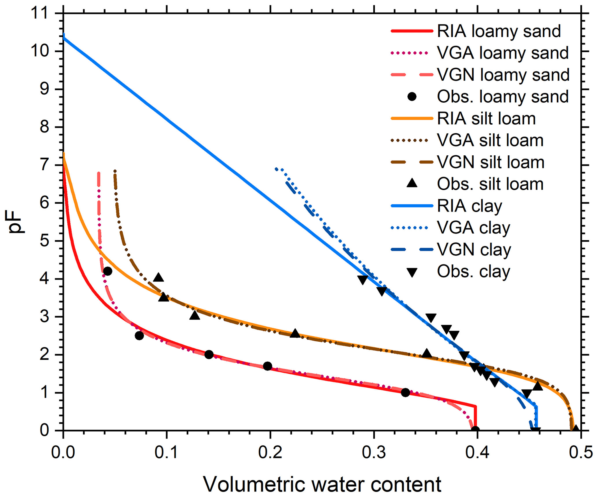
Figure 1 Soil water retention data of the soils used in the numerical simulations, and the retention curves fitted to these data for three parameterizations with a sigmoid midsection of the curve, including the original model by van Genuchten (1980; VGN), the modification thereof by Ippisch et al. (2006; VGA), and a further modification introduced in this paper (RIA).

Corrections for the conductivity curve were proposed by Vogel et al. (2001), Schaap and van Genuchten (2006), and Iden et al. (2015), but these leave the effect of the non-physical, very large pores on the SWRC intact and create an inconsistency between the retention model and the conductivity model. For instance, Iden et al. (2015) clipped the integral in the conductivity function at a matric potential h_c somewhat below zero. In the range between h_c and zero, their modified unsaturated hydraulic conductivity increased linearly with the water content (Iden et al., 2015; Fig. 1), which is not physically realistic because the pore sizes that are being filled are increasing in size, according to Eq. (1) or its multimodal version (Peters et al., 2011). Only Ippisch et al. (2006) addressed the underlying problem in the SWRC by introducing a non-zero air entry value, thereby eliminating excessively large pores whilst maintaining the mathematical consistency between the expressions for the retention and the conductivity curves. In doing so, they sacrificed the continuity of the derivative of the VGN curve. Iden et al. (2015) suspected this would pose a challenge to a numerical solution of Richards' equation, but Ippisch et al.'s (2006) numerical simulations ran without difficulty. Their equation scaled the sigmoid curve by its value at the air entry value h_ae (L) and introduced a saturated section for h>h_ae.

$$\begin{array}{}\text{(3)}& \mathit{\theta }\left(h\right)=\left\{\begin{array}{ll}{\mathit{\theta }}_{\mathrm{r}}+({\mathit{\theta }}_{\mathrm{s}}-{\mathit{\theta }}_{\mathrm{r}}){\left(\frac{\mathrm{1}+\mathrm{|}\mathit{\alpha }h{\mathrm{|}}^n}{\mathrm{1}+\mathrm{|}\mathit{\alpha }{h}_{\text{ae}}{\mathrm{|}}^n}\right)}^{\frac{\mathrm{1}}{n}-\mathrm{1}},& h\le h_{\text{ae}}\\ {\mathit{\theta }}_{\mathrm{s}},& h>h_{\text{ae}}.\end{array}\right.\end{array}$$

This function is denoted as VGA below.

The smooth, sigmoidal shape of VGN resembles many observed curves for which the data points in the wet range were obtained by equilibrating vertically placed cylindrical soil samples at well-defined matric potentials and determining the corresponding water content by weighing the sample (Klute, 1986, p. 644–647). Liu and Dane (1995) took into account the vertical variation in the water content in such samples and demonstrated that a power law SWRC with a well-defined air entry matric value but without inflection point can produce a sigmoid-type apparent SWRC if the non-uniform distribution of water in the sample is ignored. A series of data points suggesting that a smooth SWRC, therefore, does not intrinsically contradict the existence of a discrete non-zero air entry value, corroborating the correction to VGN by Ippisch et al. (2006).

Madi et al. (2018) generalized the analysis of Ippisch et al. (2006) and applied it to 18 parameterizations of the SWRC to verify that the slope of the hydraulic conductivity near saturation would remain finite. Apart from Eq. (3), only the expressions developed by Brooks and Corey (1964; denoted as BCO), Fayer and Simmons (1995; denoted as FSB), and the junction model of Rossi and Nimmo (1994; denoted as RNA) satisfied this requirement. In the latter case, a modification that smoothed the curve near saturation needed to be removed. All of these equations have a power law relationship between the water content and the matric potential and, therefore, do not have the sigmoid shape of VGN and VGA.

In a separate development, several researchers argued that, in the dry range, water is bound to the soil by adsorptive rather than capillary forces. Usually, a logarithmic term that allowed the adsorbed water content to go to zero at a prescribed matric potential was added to a capillary term. The former would dominate in the dry range and become negligible as the soil became wetter (e.g., Campbell and Shiozawa, 1992; Fayer and Simmons, 1995; Khlosi et al., 2006; Peters, 2013). The logarithmic relationship was based on the sorption theory of Bradley (1936). It removed the asymptote and the associated problem of the non-converging integral of the SWRC that Fuentes et al. (1991) warned about. Rossi and Nimmo (1994) presented a junction model in which a critical matric potential separated purely capillary-bound water from solely adsorbed water. The modified junction model of Rossi and Nimmo (1994) is as follows:

$$\begin{array}{}\text{(4)}& \mathit{\theta }\left(h\right)=\left\{\begin{array}{ll}{\mathit{\theta }}_{\mathrm{s}}\mathit{\beta }\ln \left(\frac{h_{\mathrm{d}}}{h}\right),& h_{\mathrm{d}}\le h\le h_{\mathrm{j}}\\ {\mathit{\theta }}_{\mathrm{s}}{\left(\frac{h_{\mathrm{0}}}{h}\right)}^{\mathit{\lambda }},& h_{\mathrm{j}}\le h\le h_{\mathrm{i}}\\ {\mathit{\theta }}_{\mathrm{s}}\left[\mathrm{1}-c{\left(\frac{h}{h_{\mathrm{0}}}\right)}^{\mathrm{2}}\right],& h_{\mathrm{i}}\le h\le \mathrm{0}.\end{array}\right.\end{array}$$

The first (dry) branch is logarithmic, with h_d (L) being the matric potential at which the water content reaches zero, and β is a shape parameter. The middle branch is the power law adopted from Brooks and Corey (1964; without smoothing near saturation), where λ is a shape parameter, and h₀ (L) is a fitting parameter. The final (wet) branch is a parabolic correction to avoid a discontinuity in the derivative at the air entry value, with parameter c being a function of λ and h₀ (Hutson and Cass, 1987). Madi et al. (2018) pointed out that this correction puts such strict constraints on the parameters of the conductivity curve that the usual models are ruled out. The first and middle branch are joined at h_j (L), and the middle and final branch are joined at h_i (L). Rossi and Nimmo (1994) reduced the number of fitting parameters by requiring that the water contents and the first derivatives of the branches match at h_j and h_i. This junction model avoids the problem of many of the other models that would have some capillary-bound water still present in the soil below the matric potential at which the adsorbed water content had gone to zero.

As noted above, the introduction of a non-zero air entry value by Ippisch et al. (2006) eliminated the unphysically large slopes of the hydraulic conductivity according to Mualem (1976). The approach of Rossi and Nimmo (1994) resolved the issue of the asymptotic behaviour in the dry range. The objective of this paper, therefore, is to combine Rossi and Nimmo's (1994) model for the dry range with the VGA model of Ippisch et al. (2006) to arrive at a SWRC (denoted RIA) that has a non-zero air entry value, a sigmoid shape in the intermediate range, a dry branch that can reach zero water content at a finite matric potential, and, therefore, a finite integral. We will also develop a closed-form expression for the unsaturated hydraulic conductivity based on this SWRC. For completeness, a generalized expression for multimodal SWRCs will also be derived.

Together with the other functions that lead to physically acceptable behaviour of the hydraulic conductivity near saturation (BCO, FSB, RNA, and VGA), RIA will be fitted to 21 soils selected from the UNsaturated SOil hydraulic DAtabase (UNSODA; National Agricultural Library, 2015; Nemes et al., 2001) that cover a wide range of textures (Madi et al., 2018). For comparison, VGN is also included, in view of its de facto status as the standard parameterization for the SWRC. All three versions with the sigmoid shape (VGN, VGA, and RIA) will be tested in a simulation study for different combinations of soil types and climates.

2 Theory

2.1 The soil water retention curve

The junction model of Rossi and Nimmo (1994) has a SWRC with a logarithmic dry branch without a residual water content. The parameterization proposed by Ippisch et al. (2006) combines the sigmoid shape of van Genuchten (1980) with a non-zero air entry value. By setting the θ_r in Ippisch et al. (2006) to zero, we can combine the two models to give the following parameterization:

$$\begin{array}{}\text{(5)}& \mathit{\theta }\left(h\right)=\left\{\begin{array}{ll}\mathrm{0},& h\le h_{\mathrm{d}}\\ {\mathit{\theta }}_{\mathrm{s}}\mathit{\beta }\ln \left(\frac{h_{\mathrm{d}}}{h}\right),& h_{\mathrm{d}}<h\le h_{\mathrm{j}}\\ {\mathit{\theta }}_{\mathrm{s}}{\left(\frac{\mathrm{1}+\mathrm{|}\mathit{\alpha }h{\mathrm{|}}^n}{\mathrm{1}+\mathrm{|}\mathit{\alpha }{h}_{\text{ae}}{\mathrm{|}}^n}\right)}^{\frac{\mathrm{1}}{n}-\mathrm{1}},& h_{\mathrm{j}}<h\le h_{\text{ae}}\\ {\mathit{\theta }}_{\mathrm{s}},& h>h_{\text{ae}},\end{array}\right.\end{array}$$

where subscripts “d” and “ae” denote the value at which the water content reaches zero and the air entry value, respectively, and subscript “j” indicates the value at which the logarithmic and sigmoid branch are joined. The first branch ensures that no water can be present at matric potentials below h_d. The second, logarithmic, branch is identical to that of Eq. (4). The third, sigmoidal, branch, between h_j and h_ae, and fourth branch, for matric potentials larger than the air entry value, are from Eq. (3). Joining instead of adding the logarithmic and the sigmoid functions avoids potentially non-monotonic behaviour (Peters et al., 2011).

The derivative of Eq. (5) is as follows:

$$\begin{array}{}\text{(6)}& {\displaystyle \frac{\mathrm{d}\mathit{\theta }}{\mathrm{d}h}}\left(h\right)=\left\{\begin{array}{ll}\mathrm{0},& h\le h_{\mathrm{d}}\\ \frac{{\mathit{\theta }}_{\mathrm{s}}\mathit{\beta }}{h},& h_{\mathrm{d}}<h\le h_{\mathrm{j}}\\ \begin{array}{l}{\mathit{\theta }}_{\mathrm{s}}\mathit{\alpha }(n-\mathrm{1})\mathrm{|}\mathit{\alpha }h{\mathrm{|}}^{n-\mathrm{1}}\\ {\left(\mathrm{1}+\mathrm{|}\mathit{\alpha }{h}_{\text{ae}}{\mathrm{|}}^n\right)}^{\mathrm{1}-\frac{\mathrm{1}}{n}}\\ (\mathrm{1}+\mathrm{|}\mathit{\alpha }h{\mathrm{|}}^n{)}^{\frac{\mathrm{1}}{n}-\mathrm{2}}\end{array},& h_{\mathrm{j}}<h\le h_{\text{ae}}\\ \mathrm{0},& h>h_{\text{ae}}.\end{array}\right.\end{array}$$

Mass continuity dictates that the SWRC is continuous. At the air entry value, this condition is met irrespective of the parameter values. At h_j, continuity requires the following equality to hold:

$$\begin{array}{}\text{(7)}& \mathit{\beta }\ln \left({\displaystyle \frac{h_{\mathrm{d}}}{h_{\mathrm{j}}}}\right)={\left({\displaystyle \frac{\mathrm{1}+\mathrm{|}\mathit{\alpha }{h}_{\mathrm{j}}{\mathrm{|}}^n}{\mathrm{1}+\mathrm{|}\mathit{\alpha }{h}_{\text{ae}}{\mathrm{|}}^n}}\right)}^{\frac{\mathrm{1}}{n}-\mathrm{1}}.\end{array}$$

In accordance with Rossi and Nimmo (1994), we also require the derivatives at h_j to match, leading to the following:

$$\begin{array}{}\text{(8)}& \mathit{\beta }=(n-\mathrm{1})\mathrm{|}\mathit{\alpha }{h}_{\mathrm{j}}{\mathrm{|}}^n(\mathrm{1}+\mathrm{|}\mathit{\alpha }{h}_{\text{ae}}{\mathrm{|}}^n{)}^{\mathrm{1}-\frac{\mathrm{1}}{n}}{\left(\mathrm{1}+\mathrm{|}\mathit{\alpha }{h}_{\mathrm{j}}{\mathrm{|}}^n\right)}^{\frac{\mathrm{1}}{n}-\mathrm{2}}.\end{array}$$

Combining Eqs. (7) and (8) and solving for h_d gives the following:

$$\begin{array}{}\text{(9)}& h_{\mathrm{d}}=h_{\mathrm{j}}\exp \left({\displaystyle \frac{\mathrm{1}+\mathrm{|}\mathit{\alpha }{h}_{\mathrm{j}}{\mathrm{|}}^{-n}}{n-\mathrm{1}}}\right).\end{array}$$

This leaves h_ae, h_j, θ_s, α, and n as fitting parameters.

The derivation of a multimodal curve analogous to that of Durner (1994) and Zurmühl and Durner (1998) is straightforward if the values of h_ae and h_j are kept the same for all contributing terms, as follows:

$$\begin{array}{}\text{(10)}& \mathit{\theta }\left(h\right)=\left\{\begin{array}{ll}\mathrm{0},& h\le h_{\mathrm{d}}\\ {\mathit{\theta }}_{\mathrm{s}}\mathit{\beta }\ln \left(\frac{h_{\mathrm{d}}}{h}\right),& h_{\mathrm{d}}<h\le h_{\mathrm{j}}\\ {\mathit{\theta }}_{\mathrm{s}}{\sum }_{i=\mathrm{1}}^k{w}_i{\left(\frac{\mathrm{1}+\mathrm{|}{\mathit{\alpha }}_{i}h{\mathrm{|}}^{n_i}}{\mathrm{1}+\mathrm{|}{\mathit{\alpha }}_i{h}_{\text{ae}}{\mathrm{|}}^{n_i}}\right)}^{\frac{\mathrm{1}}{n_i}-\mathrm{1}},& h_{\mathrm{j}}<h\le h_{\text{ae}}\\ {\mathit{\theta }}_{\mathrm{s}},& h>h_{\text{ae}},\end{array}\right.\end{array}$$

where the modality is indicated by k. The weighting factors w_i are bounded on the interval [0,1] and their sum must equal 1 (Durner, 1994; Zurmühl and Durner, 1998). Requiring the logarithmic and the multimodal branch and their derivatives to match at h_j leads to the following:

$$\begin{array}{}\text{(11)}& \begin{array}{rl}\mathit{\beta }=& {\sum }_{i=\mathrm{1}}^k{w}_i(n_i-\mathrm{1})\mathrm{|}{\mathit{\alpha }}_i{h}_{\mathrm{j}}{\mathrm{|}}^{n_i}{\left(\mathrm{1}+\mathrm{|}{\mathit{\alpha }}_i{h}_{\text{ae}}{\mathrm{|}}^{n_i}\right)}^{\mathrm{1}-\frac{\mathrm{1}}{n_i}}\\ & \cdot {\left(\mathrm{1}+\mathrm{|}{\mathit{\alpha }}_i{h}_{\mathrm{j}}{\mathrm{|}}^{n_i}\right)}^{\frac{\mathrm{1}}{n_i}-\mathrm{2}},\end{array}\end{array}$$

and to the following:

$$\begin{array}{}\text{(12)}& h_{\mathrm{d}}=h_{\mathrm{j}}\exp \left[{\displaystyle \frac{\mathit{\left\{}\begin{array}{l}{\sum }_{i=\mathrm{1}}^k{w}_i{\left(\mathrm{1}+\mathrm{|}{\mathit{\alpha }}_i{h}_{\text{ae}}{\mathrm{|}}^{n_i}\right)}^{\mathrm{1}-\frac{\mathrm{1}}{n_i}}\\ \cdot {\left(\mathrm{1}+\mathrm{|}{\mathit{\alpha }}_i{h}_{\mathrm{j}}{\mathrm{|}}^{n_i}\right)}^{\frac{\mathrm{1}}{n_i}-\mathrm{1}}\end{array}\mathit{\right\}}}{\mathit{\left\{}\begin{array}{l}{\sum }_{i=\mathrm{1}}^k{w}_i(n_i-\mathrm{1})\mathrm{|}{\mathit{\alpha }}_i{h}_{\mathrm{j}}{\mathrm{|}}^{n_i}\\ \cdot {\left(\mathrm{1}+\mathrm{|}{\mathit{\alpha }}_i{h}_{\text{ae}}{\mathrm{|}}^{n_i}\right)}^{\mathrm{1}-\frac{\mathrm{1}}{n_i}}\\ \cdot {\left(\mathrm{1}+\mathrm{|}{\mathit{\alpha }}_i{h}_{\mathrm{j}}{\mathrm{|}}^{n_i}\right)}^{\frac{\mathrm{1}}{n_i}-\mathrm{2}}\end{array}\mathit{\right\}}}}\right].\end{array}$$

The fitting parameters are h_ae, h_j, θ_s, α_i, n_i, and w_i.

2.2 The unsaturated hydraulic conductivity curve

The primary focus of this paper is on the SWRC. Nevertheless, it is worthwhile to find a closed-form expression for the unsaturated hydraulic conductivity that can be used in association with Eq. (5). Kosugi (1999) proposed the following conductivity model (see also Ippisch et al., 2006):

$$\begin{array}{}\text{(13)}& K\left(h\right)=K\left(h\right(S_{\mathrm{e}}\left)\right)=\left\{\begin{array}{ll}{K}_{\mathrm{s}}{S}_{\mathrm{e}}^{\mathit{\tau }}{\left(\frac{{\int }_{-\mathrm{\infty }}^{h\left(S_{\mathrm{e}}\right)}\mathrm{|}h{\mathrm{|}}^{-\mathit{\kappa }}\frac{\mathrm{d}S}{\mathrm{d}h}\mathrm{d}h}{{\int }_{-\mathrm{\infty }}^{h_{\text{ae}}}\mathrm{|}h{\mathrm{|}}^{-\mathit{\kappa }}\frac{\mathrm{d}S}{\mathrm{d}h}\mathrm{d}h}\right)}^{\mathit{\gamma }},& h<h_{\text{ae}}\\ K_{\mathrm{s}},& h\ge h_{\text{ae}},\end{array}\right.\end{array}$$

with γ, κ, and τ denoting shape parameters, S_e denoting the degree of saturation ($\mathit{\theta }-{\mathit{\theta }}_{\mathrm{r}})/({\mathit{\theta }}_{\mathrm{s}}-{\mathit{\theta }}_{\mathrm{r}}$), and S representing a variable running over all values of the degree of saturation from zero to its actual value S_e. Mualem's (1976) conductivity model is a special case of Eq. (13), with γ=2, κ=1, and τ=0.5. Madi et al. (2018) give parameter combinations for additional models.

The integrals in Eq. (13) that arise when Eq. (6) is used to find $\mathrm{d}S/\mathrm{d}h$ can be evaluated analytically if κ=1. The resulting conductivity function is as follows:

$$\begin{array}{}\text{(14a)}& K\left(h\right)=\left\{\begin{array}{ll}\mathrm{0},& h\le h_{\mathrm{d}}\\ \begin{array}{l}{K}_{\mathrm{s}}{\left(\mathit{\beta }\ln \mathrm{|}\frac{h_{\mathrm{d}}}{h}\mathrm{|}\right)}^{\mathit{\tau }}\\ \cdot {\left[\frac{\frac{\mathit{\beta }}{\mathrm{|}{h}_{\mathrm{d}}\mathrm{|}}-\frac{\mathit{\beta }}{\mathrm{|}h\mathrm{|}}}{\mathit{\left\{}\begin{array}{l}\frac{\mathit{\beta }}{\mathrm{|}{h}_{\mathrm{d}}\mathrm{|}}-\frac{\mathit{\beta }}{\mathrm{|}{h}_{\mathrm{j}}\mathrm{|}}+\frac{\mathrm{|}\mathit{\alpha }{h}_{\text{ae}}{\mathrm{|}}^n}{\mathrm{|}{h}_{\text{ae}}\mathrm{|}}\\ -{\left(\mathrm{1}+\mathrm{|}\mathit{\alpha }{h}_{\text{ae}}{\mathrm{|}}^n\right)}^{\mathrm{1}-\frac{\mathrm{1}}{n}}\\ F\left(h_{\mathrm{j}}\right)\end{array}\mathit{\right\}}}\right]}^{\mathit{\gamma }}\end{array},& h_{\mathrm{d}}<h\le h_{\mathrm{j}}\\ \begin{array}{l}{K}_{\mathrm{s}}{\left(\frac{\mathrm{1}+\mathrm{|}\mathit{\alpha }h{\mathrm{|}}^n}{\mathrm{1}+\mathrm{|}\mathit{\alpha }{h}_{\text{ae}}{\mathrm{|}}^n}\right)}^{\frac{\mathit{\tau }}{n}-\mathit{\tau }}\\ \cdot {\left\{\frac{\mathit{\left\{}\begin{array}{l}\frac{\mathit{\beta }}{\mathrm{|}{h}_{\mathrm{d}}\mathrm{|}}-\frac{\mathit{\beta }}{\mathrm{|}{h}_{\mathrm{j}}\mathrm{|}}\\ +{\left(\mathrm{1}+\mathrm{|}\mathit{\alpha }{h}_{\text{ae}}{\mathrm{|}}^n\right)}^{\mathrm{1}-\frac{\mathrm{1}}{n}}\\ \cdot \left[F\right(h)-F(h_{\mathrm{j}}\left)\right]\end{array}\mathit{\right\}}}{\mathit{\left\{}\begin{array}{l}\frac{\mathit{\beta }}{\mathrm{|}{h}_{\mathrm{d}}\mathrm{|}}-\frac{\mathit{\beta }}{\mathrm{|}{h}_{\mathrm{j}}\mathrm{|}}+\frac{\mathrm{|}\mathit{\alpha }{h}_{\text{ae}}{\mathrm{|}}^n}{\mathrm{|}{h}_{\text{ae}}\mathrm{|}}\\ -{\left(\mathrm{1}+\mathrm{|}\mathit{\alpha }{h}_{\text{ae}}{\mathrm{|}}^n\right)}^{\mathrm{1}-\frac{\mathrm{1}}{n}}\\ \cdot F\left(h_{\mathrm{j}}\right)\end{array}\mathit{\right\}}}\right\}}^{\mathit{\gamma }}\end{array},& h_{\mathrm{j}}<h\le h_{\text{ae}}\\ K_{\mathrm{s}},& h>h_{\text{ae}},\end{array}\right.\end{array}$$

where, in the following:

$$\begin{array}{}\text{(14b)}& F\left(h\right)={\displaystyle \frac{\mathrm{|}\mathit{\alpha }h{\mathrm{|}}^n(\mathrm{1}+\mathrm{|}\mathit{\alpha }h{\mathrm{|}}^n{)}^{\frac{\mathrm{1}}{n}-\mathrm{1}}}{\mathrm{|}h\mathrm{|}}}.\end{array}$$

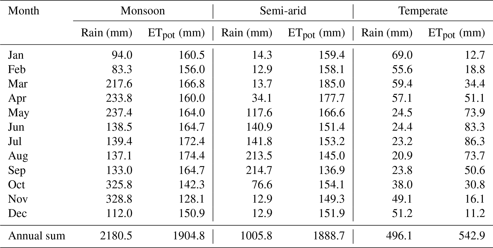
Table 1 Average cumulative monthly and annual rainfall and potential evapotranspiration of the three test climates calculated from 1000 years of generated weather records.

If only the hydraulic conductivity at saturation is available, one can use the values for α and n of the water retention curve and fix parameters γ and τ according to one of several conductivity models (Madi et al., 2018) to define an unsaturated hydraulic conductivity curve, but this is not recommended. It is better to have additional data points of the hydraulic conductivity curve so that parameters γ and τ, and perhaps even conductivity-specific values of α and n, can be fitted directly to the conductivity data.

Equations (14a) and (14b) have an advantage in that they can be expressed in closed form, but they do not account for non-capillary flow in dry soils, vapour flow, or sequences of evaporation and condensation in soils with pockets of water and soil air. Hence, they are of limited value for water flows in dry soils. For such conditions, more sophisticated conductivity could be selected; for instance, using the framework presented by Weber et al. (2019).

The conductivity function associated with the multimodal soil water retention function cannot be expressed in a closed form. For that case, the degree of saturation for any h can be found with Eq. (10), and the corresponding hydraulic conductivity determined with Eq. (13) or another conductivity model.

3 Materials and methods

We selected 21 soils from the UNSODA database that had sufficient retention data and also covered the textures represented in UNSODA. We then fitted Eq. (5) to these soils using a shuffled complex evolution algorithm (see Madi et al., 2018, and Appendix C for details of the algorithm and the fitting procedure). We slightly modified the fitting code used by Madi et al. (2018) to generate output that can more readily be converted to the Mater.in input file for Hydrus-1D, the numerical model used in this study. We therefore refitted BCO, FSB, RNA, VGN, and VGA as well.

One-dimensional simulations for all combinations of three soils and three climates were carried out to examine how the choice of parameterization affected fluxes at the soil surface and in the subsoil. The model Hydrus-1D, version 4.16.0110 (Šimůnek et al., 2013; PC-Progress, 2019), was used for this purpose. The selected soils were a loamy sand (UNSODA identifier – 2104), a silty loam (3261), and a clay (1181). Weather records were generated from climate parameters based on weather data from Colombo (Sri Lanka; monsoon climate), Tamale (Ghana; semi-arid climate), and Ukkel (Belgium; temperate climate). Table 1 gives the most relevant statistics of the weather records. In order to highlight the effects of the air entry value and the logarithmic dry end of the SWRC, we used the sigmoidal VGN, VGA, and RIA parameterizations in the simulations. The Supplement details the generation of the weather records, the set-up of the simulations, and the simulation results.

Table 2 Parameters of the fit to data of the three parameterizations of the soil water retention curve used for the numerical simulations.

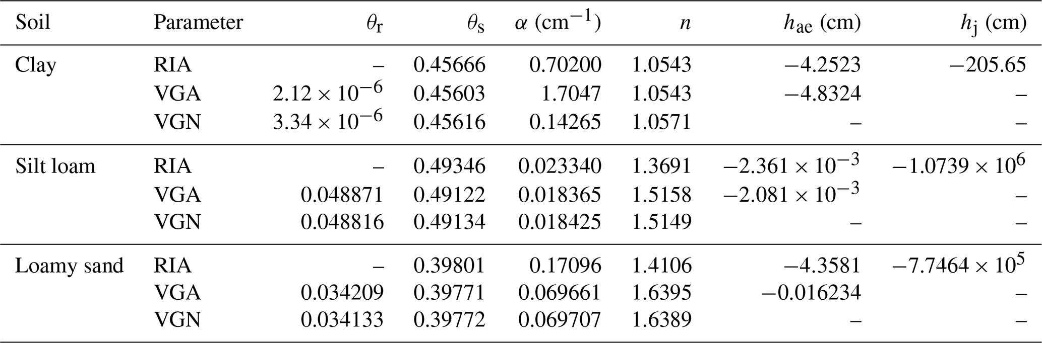
The different parameterizations of the SWRCs (Table 2; Fig. 1) were used to generate tables of the soil water retention and conductivity curves that were provided as input to Hydrus-1D. Equations (14a) and (14b), with γ=2 and τ=0.5 (Mualem, 1976), were used to generate relative hydraulic conductivities (scaled by K_s). These were converted to unscaled conductivities (Fig. 2), by multiplying with the K_s value according to the UNSODA database, and then included in the tables.

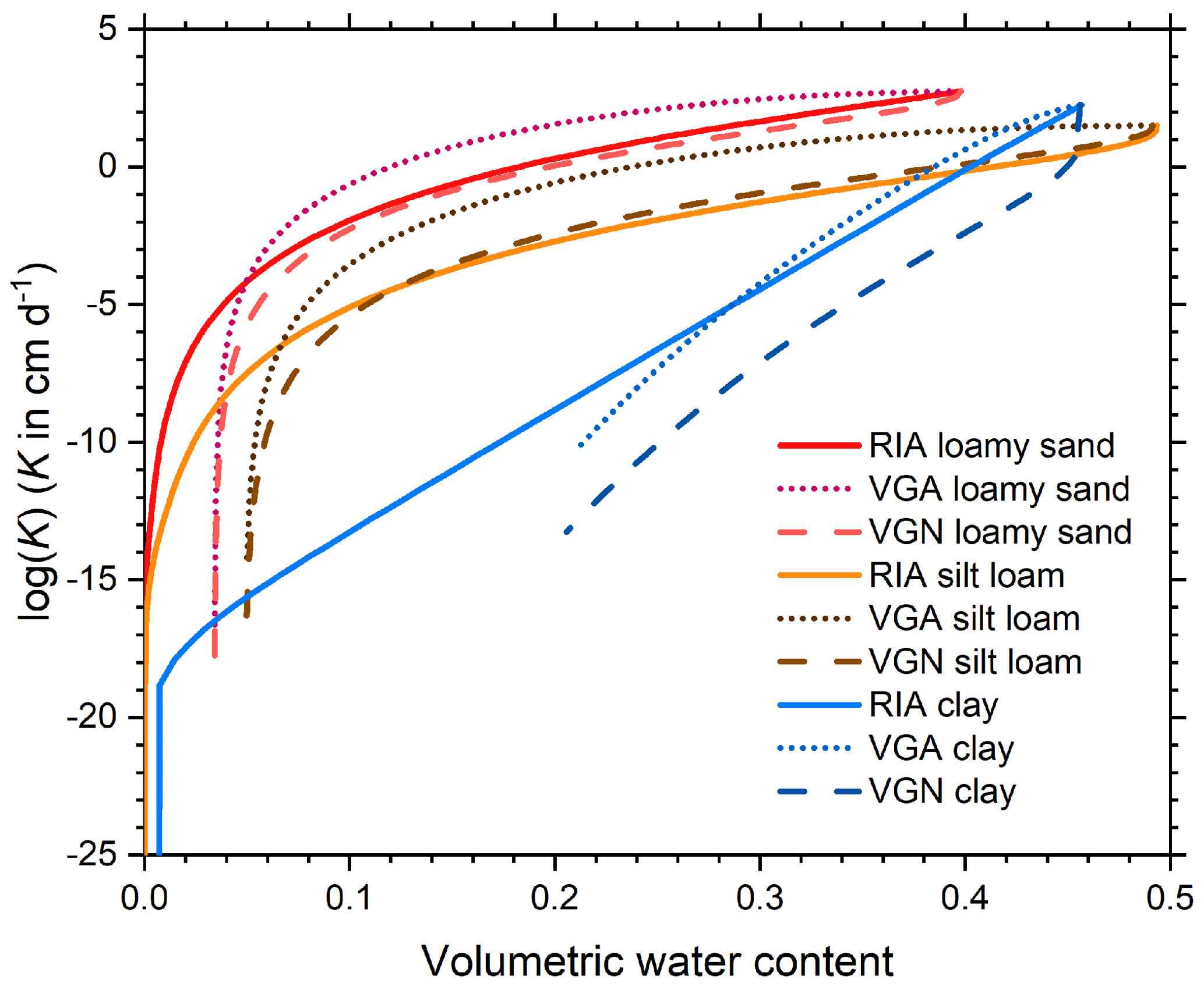
Figure 2 The unsaturated soil hydraulic conductivity curves derived from the fitted retention curves depicted in Fig. 1 and scaled by soil-specific values of the hydraulic conductivity at saturation.

For the clay soil, the recorded value (178 cm d⁻¹) was such that it can be assumed that macropore flow contributed to its value. We therefore also ran simulations with a K_s value of 1.25 cm d⁻¹. This value was adopted from soil 1182, from the UNSODA database, from the same location.

4 Results and discussion

4.1 Fitted curves for 21 soils

The fitted parameter values (Tables C1–C4) and the associated curves (Figs. C2–C5) are presented in Appendix C. The extra parameter of RIA compared to RNA and FSB gives it a clear advantage in fitting the full water content range. The sigmoid shape of RIA provides a better fit near the air entry value, while still providing good fits of the drier data points (e.g. 1121 in Fig. C3; all soils in Figs. C4–C5). In the wet range, the sigmoid curves (VGN, VGA, and RIA) outperform the power law curves (BCO, FSB, and RNA). In almost all cases, VGA and RIA look very similar. Figure C3 shows multimodality in the data for five out of six soils that cannot be reproduced by any of the parameterizations.

Many of the UNSODA soils have one retention data point at saturation and the next at h = −10 cm. The air entry value of many sandy soils is within that range. The fitting routine struggles to fit h_ae to these data for VGA and RIA because the sigmoid shape of the van Genuchten parameterization has such flexibility that it can fit the intermediate range well for a range of h_ae values. We therefore recommend making θ(h) measurements at one or two matric potentials between zero and −10 cm for coarse-textured soils.

A total of 11 of the 21 soils have residual water contents for VGN and/or VGA that exceed 0.05 (up to 0.263), mostly in loamy sands, loams, and clays (Tables C1–C4). All of these and several others have dry-end data points with water contents that appear too high (Figs. C2–C5). These water contents may have been overestimated due to the lack of equilibrium reported by Bittelli and Flury (2009). The parameterizations without asymptote (FSB, RNA, and RIA) generally have more plausible fits, based on visual inspection of the graphs, but because they do not follow the upward tail of the data in the dry end, their root mean square error (RMSE) values for the cases with suspicious dry-end data points are larger than those of VGN and VGA (Tables C5–C8).

Especially for fine-textured soils, the lack of data points for air dryness or oven dryness (Figs. C3–C5) causes the fitting procedure to treat θ_r for the asymptotic dry branches and h_d for the logarithmic dry branches as pure fitting parameters for the drier range of the data. This range exceeds pF4.2 in only one case, and in several cases likely suffers from lack of equilibrium (Bittelli and Flury, 2009). This leads to unrealistically high values for both in many cases. If applications are envisioned for which low water contents are expected, it would be better to have some data in the dry range and ensure that equilibrium has been achieved before fitting RIA.

Table 3 Parameters of the fit to the pressure plate data and a combination of the pressure plate and dew point data of Bittelli and Flury (2009).

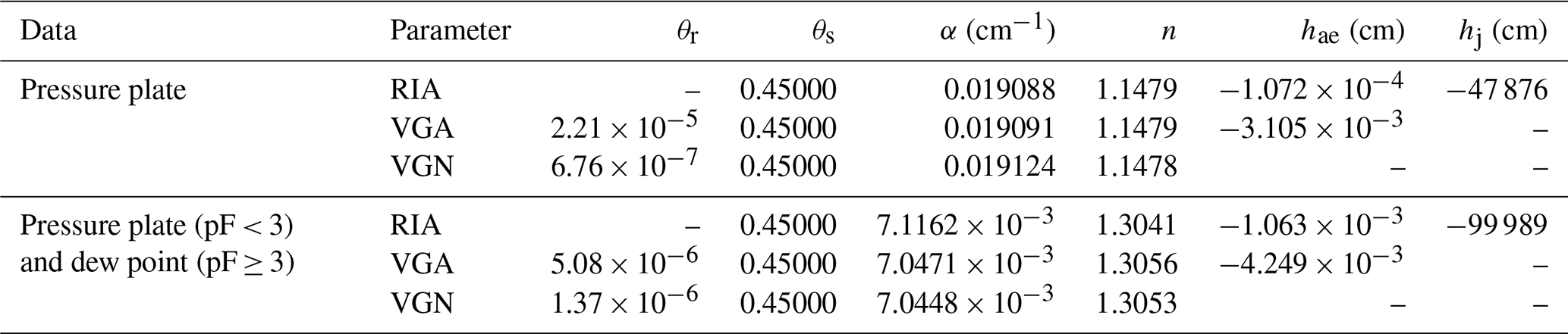
We tested this on the data of Bittelli and Flury (2009) for undisturbed samples taken at 0.15 m depth. We fitted RIA, VGA, and VGN with θ_s fixed at 0.45 to their pressure plate data (which were unreliable in the dry range) and a combination of pressure plate data for matric potentials larger than −1000 cm H₂O (pF3.0) and dew point data for higher pF values (Table 3). Figure 3 shows that all three parameterizations gave good fits for both data sets, and that the dry-end data points affect the entire SWRC. It is important to note that the pF value of h_d for the combination of pressure plate and dew point data equals 6.428, close to the oven-dry value of pF6.8 approximated by most sample-drying ovens, according to Schneider and Goss (2012).

Figure 3 Soil water retention data obtained by Bittelli and Flury (2009) from samples placed on pressure plates (i.e. p.p. data) or from a combination of pressure plates for the wettest three data points and dew point measurements for the driest six data points (i.e. p.p. and d.p. data). The curves show the fits of the soil water retention curves according to van Genuchten (1980; VGN), Ippisch et al. (2006; VGA), and Eq. (5) (RIA).

If reliable data in the dry range are not available but a realistic fit in the dry range is necessary, one could add a virtual data point with zero water content at pF6.8, according to Schneider and Goss (2012), and give it a high weight to force the fitting algorithm to approximate it closely. We did not do so here to be able to observe how the various parameterizations perform on frequently reported data ranges.

Figure C5 showcases a peculiarity of FSB. The original version by Fayer and Simmons (1995) allowed capillary-bound water to be present even if the adsorbed water content was down to zero. We adopted the correction by Madi et al. (2018; Eq. S12a) that forced the amount of water bound by capillary forces to zero if the adsorbed water content reaches zero at pF6.8. In the case of clay soils, the parameter values are such that a substantial amount of capillary-bound water is still present at pF6.8, leading to a sudden cut-off at pF6.8.

The hydraulic conductivity curves based on water retention curve parameters and K_s very poorly match the data in most cases (Figs. C6–C9), which confirms that it is better to fit conductivity parameters to conductivity data instead of relying on values prescribed by theoretical models. We note here that all but one (soil 4450; Fig. C8) set of unsaturated conductivity data were obtained in the field, while all retention data were laboratory data on drying samples. The reported K_s values were probably measured in a separate experiment (possibly in the laboratory) in which case a mismatch between K_s and the unsaturated conductivity data is to be expected. The poor match with field data notwithstanding, the graphs can be used to study the effect of the parameterization on the shape of the K(θ) curve. The comparison between measured and modelled shapes of the conductivity curves is inconclusive.

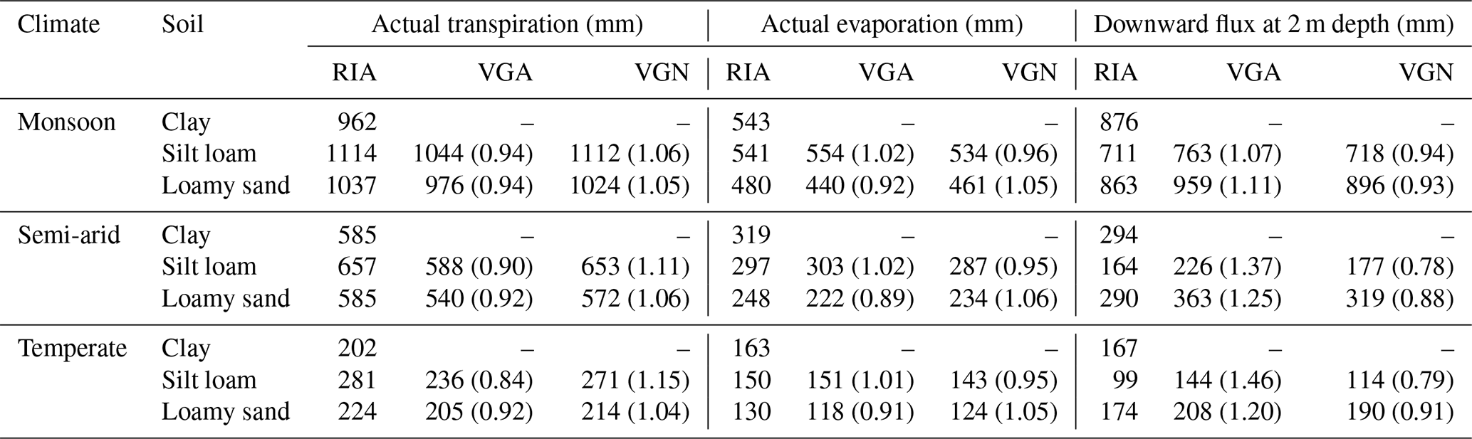
Table 4 Average of the annual sums of the actual transpiration and evaporation and of the outflow across the lower boundary of the simulated soil profiles. The averages were calculated for the final 6 years of the simulation periods. The values in parentheses are scaled with respect to the corresponding value for RIA.

In many soils, regardless of texture, RIA's K(θ) curve drops off much slower in the dry range than those of VGN and VGA (Figs. C6–C9), a consequence of the ability of the underlying SWRC to reach zero water content at a finite matric potential. Near saturation, RIA's K(θ) curve often drops off sharply before levelling off, in stark contrast to that of VGA, which remains high in the wet range. Given the similarity in the θ(h) curves of VGA and RIA, the difference in their K(θ) curves is remarkable. RIA's K(θ) curve is the only one that can drop off sharply near saturation, level out somewhat in the mid range, and drop ever more sharply in the dry range. It is below many of the other curves in the wet and mid range, and above most of them in the dry range.

Peters et al. (2011) developed parameter constraints to ensure physically plausible shapes of the SWRC and the conductivity curve. For FSB, the criterion for non-monotonicity of the conductivity curve is not met for soil 4450 (Fig. C8), resulting in K increasing with decreasing water content near saturation.

4.2 Model simulations

In total, 21 out of 36 combinations of the soil–climate parameterization ran to completion. Runoff did not occur in any of the successful model runs. Convergence was not achieved for any of the runs for the clay soil with the reduced K_s value. For the clay soil with the high K_s value, only RIA ran to completion. The discontinuity of the first derivative at the air entry value did not cause numerical problems. In fact, the replacement of any parametric expression by a look-up table creates a discontinuity in the first derivative at every point of the look-up table.

Table 4 lists the main mean annual fluxes calculated from the simulation study. The median flux was produced by RIA for all combinations of soil and climate. The mean annual actual transpiration between the three parameterizations differed by more than 10 % from the median only for the silt loam under a temperate climate. The actual evaporation only deviated more than 10 % for the loamy sand under a semi-arid climate. The amount of water leaving the soil profile differed substantially between parameterizations for the semi-arid and temperate climate, especially for VGA (20 %–46 % deviation from the median).

The daily data revealed significant differences on smaller timescales that will be relevant if reactive solute transport is of interest (see the Supplement). The fluxes generated by the VGA parameterizations responded more quickly and strongly to the rainfall signal, with VGN and RIA giving a more delayed and smooth response. The SWRCs (Fig. 1) offer no explanation for this, but Fig. 2 shows that VGA's hydraulic conductivity in the wet and intermediate water content range for all three soils is considerably higher than that of VGN and RIA, except for clay, where it is only moderately higher than RIA's and drops below RIA at a water content of 0.28. Thus, small differences between SWRCs can have a significant influence on soil water flow simulations through the effect of their parameters on the soil hydraulic conductivity curve, an effect that the reviews by Leij et al. (1997) and Assouline and Or (2013) took into consideration to some degree, but it was not considered in several other studies that compared different parameterizations (e.g., Rossi and Nimmo, 1994; Assouline et al., 1998; Cornelis et al., 2005; Khlosi et al., 2008).

5 Summary and conclusions

The improvements incorporated in the RIA parameterization for the first time remove problems of the popular VGN model in both the wet and the dry range, while retaining the desirable sigmoid shape in the mid range. This shape allows its multimodal version to represent SWRCs with multiple humps. RIA offers a wider range of shapes for the conductivity curve than any other parameterization that does not lead to the unphysical behaviour near saturation that was revealed by Durner (1994) and Ippisch et al. (2006) for VGN and by Madi et al. (2018) for 14 other parameterizations. RIA also proved to be more robust during numerical simulations than VGN and its modification VGA, which still has a non-physical asymptote at a non-zero residual water content. The deep drainage generated by RIA was more spread out and smaller than the spiked response to rainfall produced by VGA, probably because RIA was better able to produce a conductivity curve with a substantial drop during the early stages of drying. We, therefore, hope that RIA or its multimodal version will be adopted for use in numerical simulations of soil water flow. The catalogue of parameters for 21 soils in Appendix C may be of help for such simulations.

Appendix A: List of abbreviations

BC	Brooks and Corey (1964)
BCO	Parameterization of the SWRC according to the original Brooks and Corey (1964) equation
FSB	Parameterization of the SWRC according to the BC-based version of Fayers and Simmons (1995)
RIA	Parameterization of the SWRC that combines RNA and VGA
RNA	Parameterization of the SWRC according to the junction model of Rossi and Nimmo (1994)
SWRC	Soil water retention curve
RMSE	Root mean square error
UNSODA	UNsaturated SOil hydraulic DAtabase
VGA	Parameterization of the SWRC according to Ippisch et al. (2006)
VGN	Parameterization of the SWRC according to the original van Genuchten (1980) equation

Appendix B: Assessing the near-saturation behaviour of recently developed soil water retention and hydraulic conductivity curves

Madi et al. (2018) developed a criterion that needs to be met to avoid unphysical behaviour of the unsaturated soil hydraulic conductivity curve near saturation, as follows:

$$\begin{array}{}\text{(B1)}& \underset{h\uparrow \mathrm{0}}{lim}\left(\mathrm{|}h{\mathrm{|}}^{-\mathit{\kappa }}{\displaystyle \frac{\mathrm{d}\mathit{\theta }}{\mathrm{d}h}}\right)=\mathrm{0},\end{array}$$

where κ is a fitting parameter (>0) that appears in a several parameterizations of the unsaturated soil hydraulic conductivity curve based on the capillary bundle conceptualization.

Fredlund and Xing (1994) introduced the following parameterization for the soil water retention curve:

$$\begin{array}{}\text{(B2)}& \mathit{\theta }\left(h\right)=\left[{\displaystyle \frac{-\ln \left(\mathrm{1}+\frac{\mathrm{|}h\mathrm{|}}{\mathrm{|}{h}_{\mathrm{r}}\mathrm{|}}\right)}{\ln \left(\mathrm{1}+\frac{b}{\mathrm{|}{h}_{\mathrm{r}}\mathrm{|}}\right)}}+\mathrm{1}\right]{\displaystyle \frac{{\mathit{\theta }}_{\mathrm{s}}}{{\left\{\ln \left[\mathrm{e}+{\left(\frac{\mathrm{|}h\mathrm{|}}{a}\right)}^n\right]\right\}}^m}},\end{array}$$

where the subscript “r” denotes the value when the residual water content is reached, and a (L), n, and m are fitting parameters. The first term on the right-hand side is a correction term that forces the water content to zero for $h=-b$, with b equal to 10⁷ cm (Fredlund and Xing, 1994) or 6.3 × 10⁶ cm (Wang et al., 2016). Wang et al. (2016) also modified the correction factor to give the following:

$$\begin{array}{}\text{(B3)}& \mathit{\theta }\left(h\right)=\left[{\displaystyle \frac{-\ln \left(\mathrm{1}+\frac{c\mathrm{|}h\mathrm{|}}{\mathrm{|}{h}_{\mathrm{r}}\mathrm{|}}\right)}{\ln \left(\mathrm{1}+\frac{bc}{\mathrm{|}{h}_{\mathrm{r}}\mathrm{|}}\right)}}+\mathrm{1}\right]{\displaystyle \frac{{\mathit{\theta }}_{\mathrm{s}}}{{\left\{\ln \left[\mathrm{e}+{\left(\frac{\mathrm{|}h\mathrm{|}}{a}\right)}^n\right]\right\}}^m}},\end{array}$$

where c has to be small and positive. The derivative of Eq. (B3) is as follows:

$$\begin{array}{}\text{(B4)}& \begin{array}{rl}{\displaystyle \frac{\mathrm{d}\mathit{\theta }}{\mathrm{d}h}}=& {\displaystyle \frac{-{\mathit{\theta }}_{\mathrm{s}}}{{\left\{\ln \left[\mathrm{e}+{\left(\frac{\mathrm{|}h\mathrm{|}}{a}\right)}^n\right]\right\}}^m}}\\ & \cdot \left\{{\displaystyle \frac{mn\mathrm{|}h{\mathrm{|}}^{n-\mathrm{1}}\left[\ln \left(\mathrm{1}+\frac{bc}{\mathrm{|}{h}_{\mathrm{r}}\mathrm{|}}\right)\ln \left(\mathrm{1}+\frac{c\mathrm{|}h\mathrm{|}}{\mathrm{|}{h}_{\mathrm{r}}\mathrm{|}}\right)-\mathrm{1}\right]}{a^n\left[\mathrm{e}+{\left(\frac{\mathrm{|}h\mathrm{|}}{a}\right)}^n\right]\ln \left[\mathrm{e}+{\left(\frac{\mathrm{|}h\mathrm{|}}{a}\right)}^n\right]}}\right.\\ & \left.-{\displaystyle \frac{\ln \left(\mathrm{1}+\frac{bc}{\mathrm{|}{h}_{\mathrm{r}}\mathrm{|}}\right)}{\frac{\mathrm{|}{h}_{\mathrm{r}}\mathrm{|}}{c}+\mathrm{|}h\mathrm{|}}}\right\}.\end{array}\end{array}$$

The derivative of Eq. (B2) follows by setting c equal to 1 in Eq. (B4). Combining Eq. (B4) with Eq. (B1) results in the following requirement:

$$\begin{array}{}\text{(B5)}& \underset{h\uparrow \mathrm{0}}{lim}\left[{\displaystyle \frac{{\mathit{\theta }}_{\mathrm{s}}mn}{\mathrm{e}{a}^n}}\mathrm{|}h{\mathrm{|}}^{-\mathit{\kappa }+n-\mathrm{1}}+{\displaystyle \frac{c{\mathit{\theta }}_{\mathrm{s}}\ln \left(\mathrm{1}+\frac{bc}{\mathrm{|}{h}_{\mathrm{r}}\mathrm{|}}\right)}{\mathrm{|}{h}_{\mathrm{r}}\mathrm{|}}}\mathrm{|}h{\mathrm{|}}^{-\mathit{\kappa }}.\right]=\mathrm{0}\end{array}$$

The limit goes to zero if, and only if, the exponents in both terms are positive. Hence, $\mathit{\kappa }<n-\mathrm{1}$ and κ<0. The first requirement may be met for some soils, but the second violates the physical constraint that κ cannot be negative (Madi et al., 2018). Therefore, neither Fredlund and Xing's (1994) nor Wang et al.'s (2016) parameterization lead to unsaturated hydraulic conductivity curves that exhibit physically realistic behaviour near saturation. Wang et al. (2018) added a modification to the dry end of Wang et al. (2016), and Rudiyanto et al. (2020), in turn, used Wang et al.'s (2018) curves. Because the problem near saturation was not resolved, these two hydraulic conductivity models suffer from the same problem near saturation.

Appendix C: Fitted parameters and root mean square error for six parameterizations of the soil water retention curve applied to data of 21 soils

The UNSODA soils selected for parameter fitting are grouped in Tables C1–C4, according to their texture classification, according to Twarakavi et al. (2010). Sand is a major constituent of the mineral soil in Tables C1 and C2, silt in Table C3, and clay in Table C4. Figure C1 shows the textural composition of the soils. For each soil, the parameter values for six parameterizations are given, resulting in a total of 126 SWRC parameterizations. The root mean square errors (RMSEs) for all fits are listed in Tables C5–C8. The saturated hydraulic conductivities of the soils, as given by the UNSODA database, are given in Table C9.

Table C1 The fitting parameters and their values for six parameterizations for sandy soils in the A1 and A2 classifications of Twarakavi et al. (2010) from the UNSODA database (National Agricultural Library, 2015; Nemes et al., 2001). The three-character parameterization label is explained in the main text.

Table C2 The fitting parameters and their values for six parameterizations for sandy soils in the A3 and A4 classifications of Twarakavi et al. (2010) from the UNSODA database (National Agricultural Library, 2015; Nemes et al., 2001). The three-character parameterization label is explained in the main text.

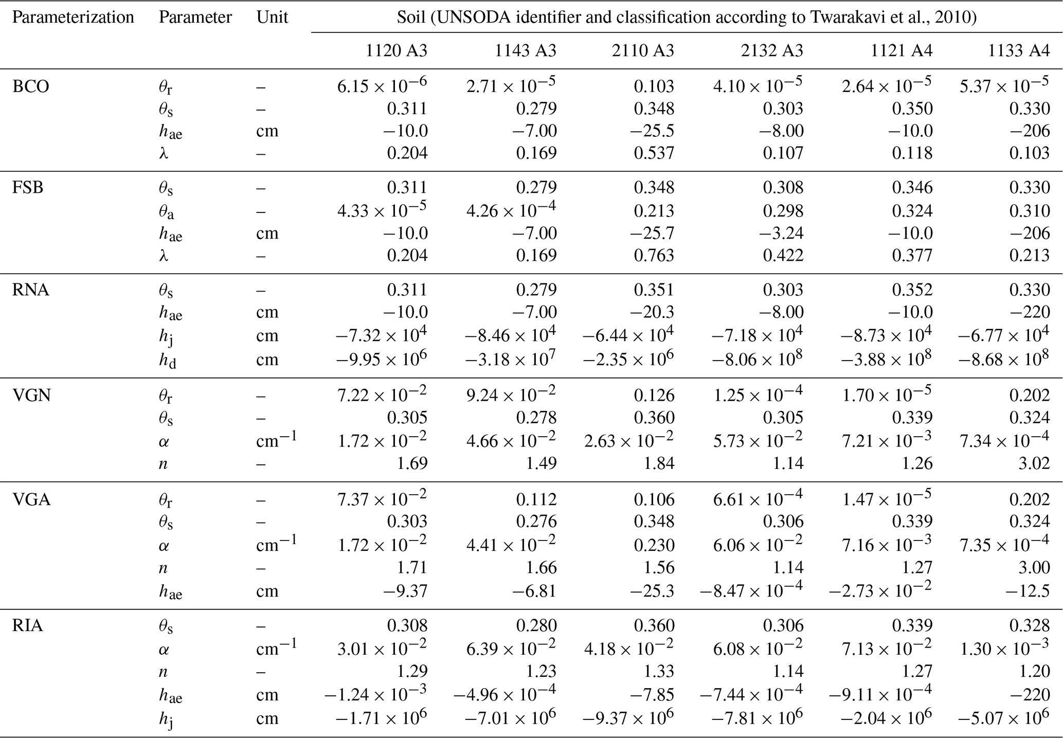
Table C3 The fitting parameters and their values for six parameterizations for silty soils from the UNSODA database (National Agricultural Library, 2015; Nemes et al., 2001). The three-character parameterization label is explained in the main text.

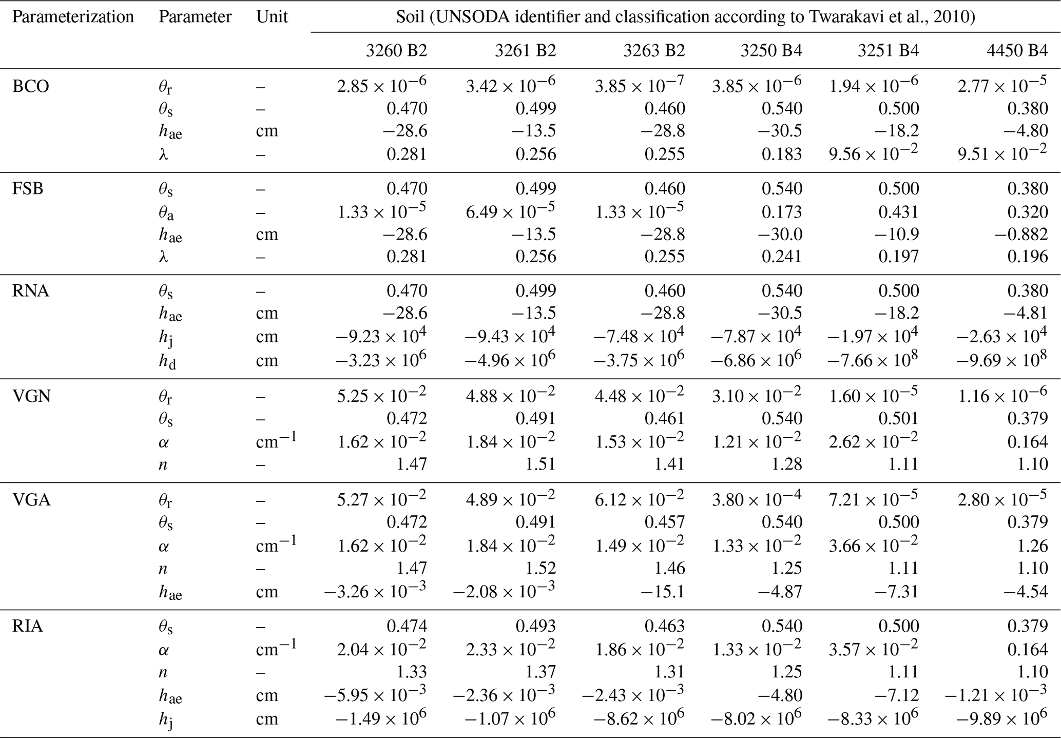
Table C4 The fitting parameters and their values for six parameterizations for clayey soils from the UNSODA database (National Agricultural Library, 2015; Nemes et al., 2001). The three-character parameterization label is explained in the main text.

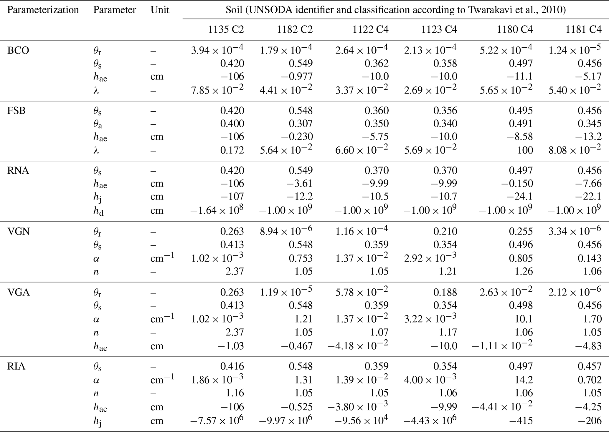
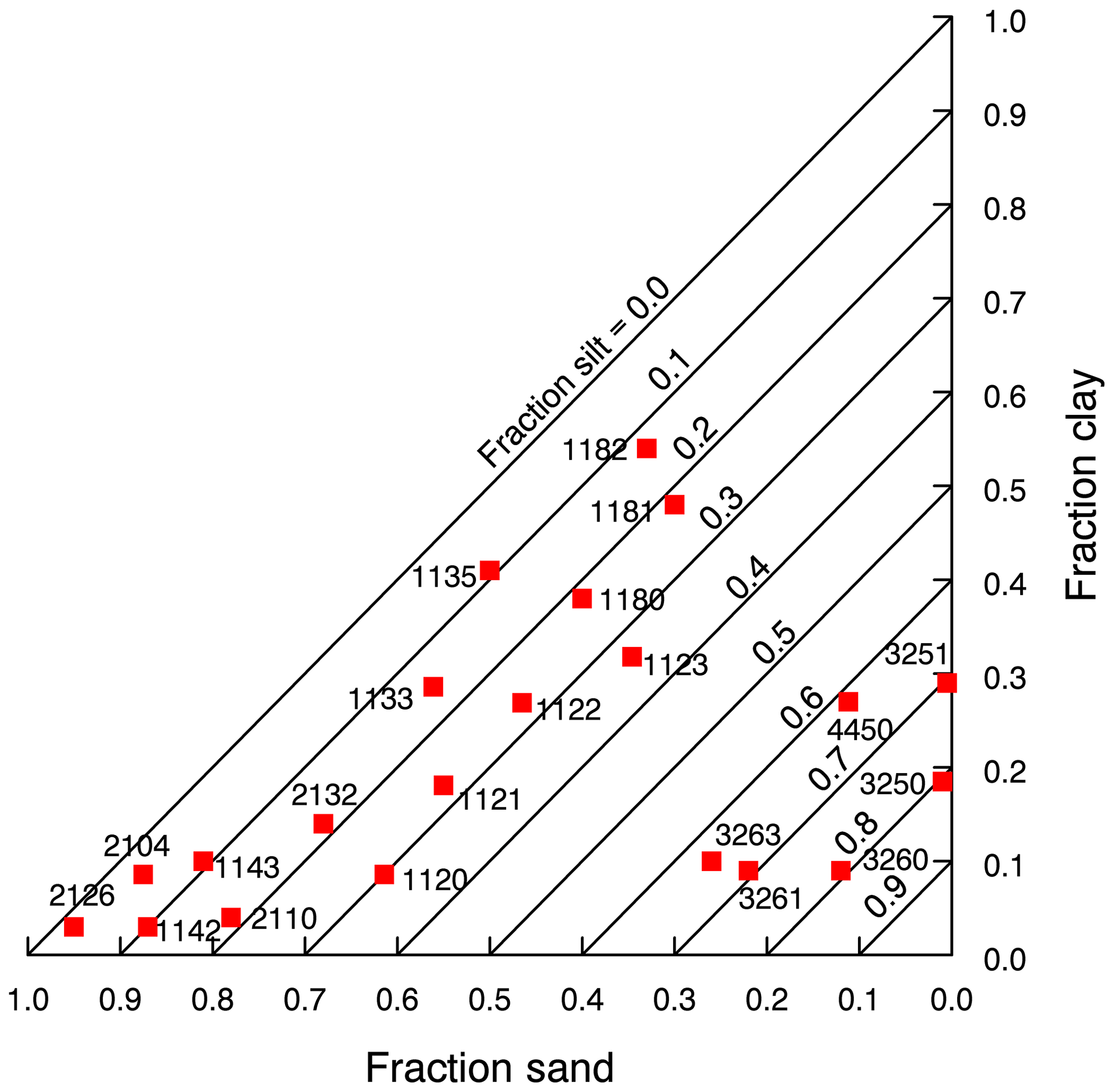
Figure C1 The positions in the texture triangle of the selected soils as indicated by their UNSODA identifier (from Madi et al., 2018).

Table C5 Root mean square errors of the parameter fits for the sandy or loamy soils (A1 and A2 soils, according to Twarakavi et al., 2010).

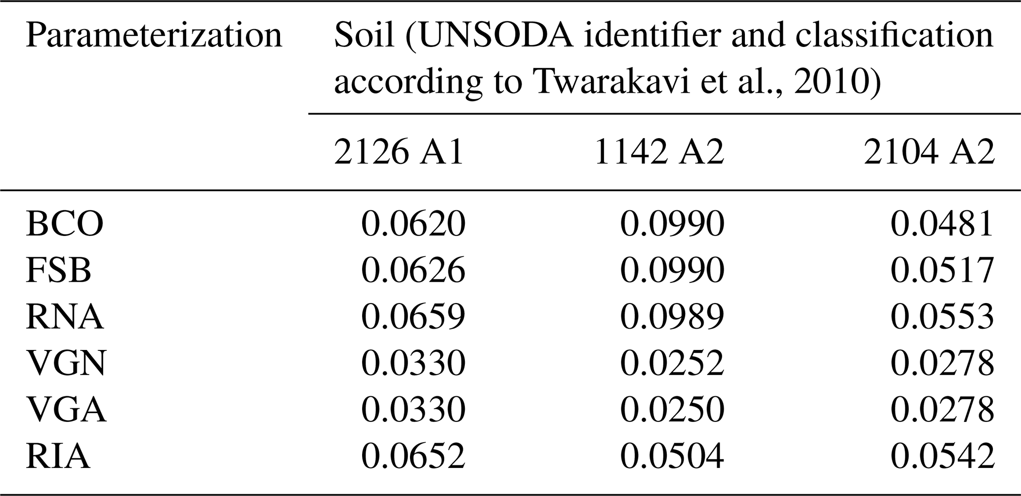
Table C6 Root mean square errors of the parameter fits for the sandy soils (A3 and A4 soils, according to Twarakavi et al., 2010).

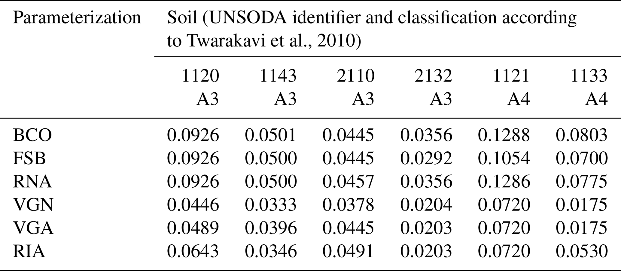
Table C7 Root mean square errors of the parameter fits for the silty soils.

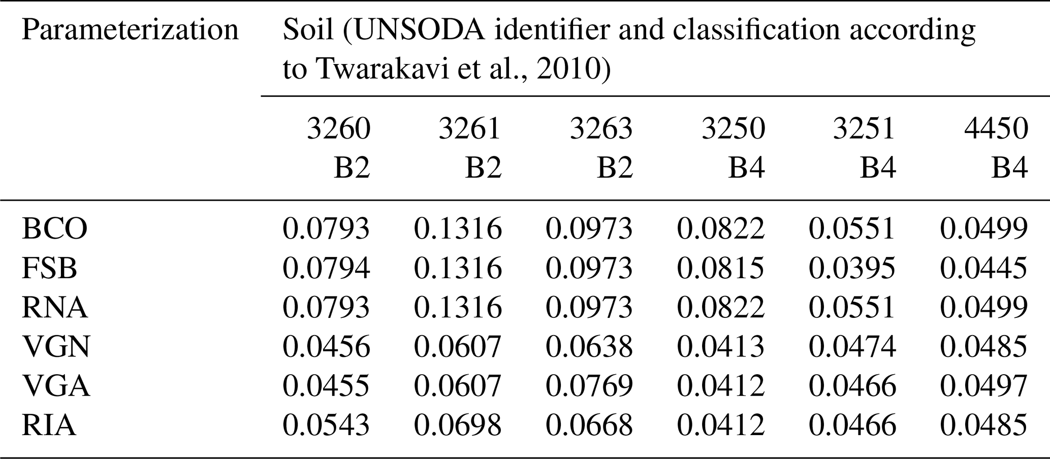
Table C8 Root mean square errors of the parameter fits for the clayey soils.

Table C9 Values for the hydraulic conductivity at saturation (K_s) for the selected soils from the UNSODA database. The soils are identified by their UNSODA identifier. Their classification according to Twarakavi et al. (2010) is also given.

Madi et al. (2018) provide an analysis of the underlying functions of all parameterizations tested here, except RIA. The meaning of all variables except λ is explained in the main text. Variable λ is the power to which the factor ($h/h_{\text{ae}}$) is raised in the power law segments of the SWRCs of BCO, FSB, and RNA. In RNA, λ is expressed as a function of the fitting parameters and, therefore, does not appear in the tables.

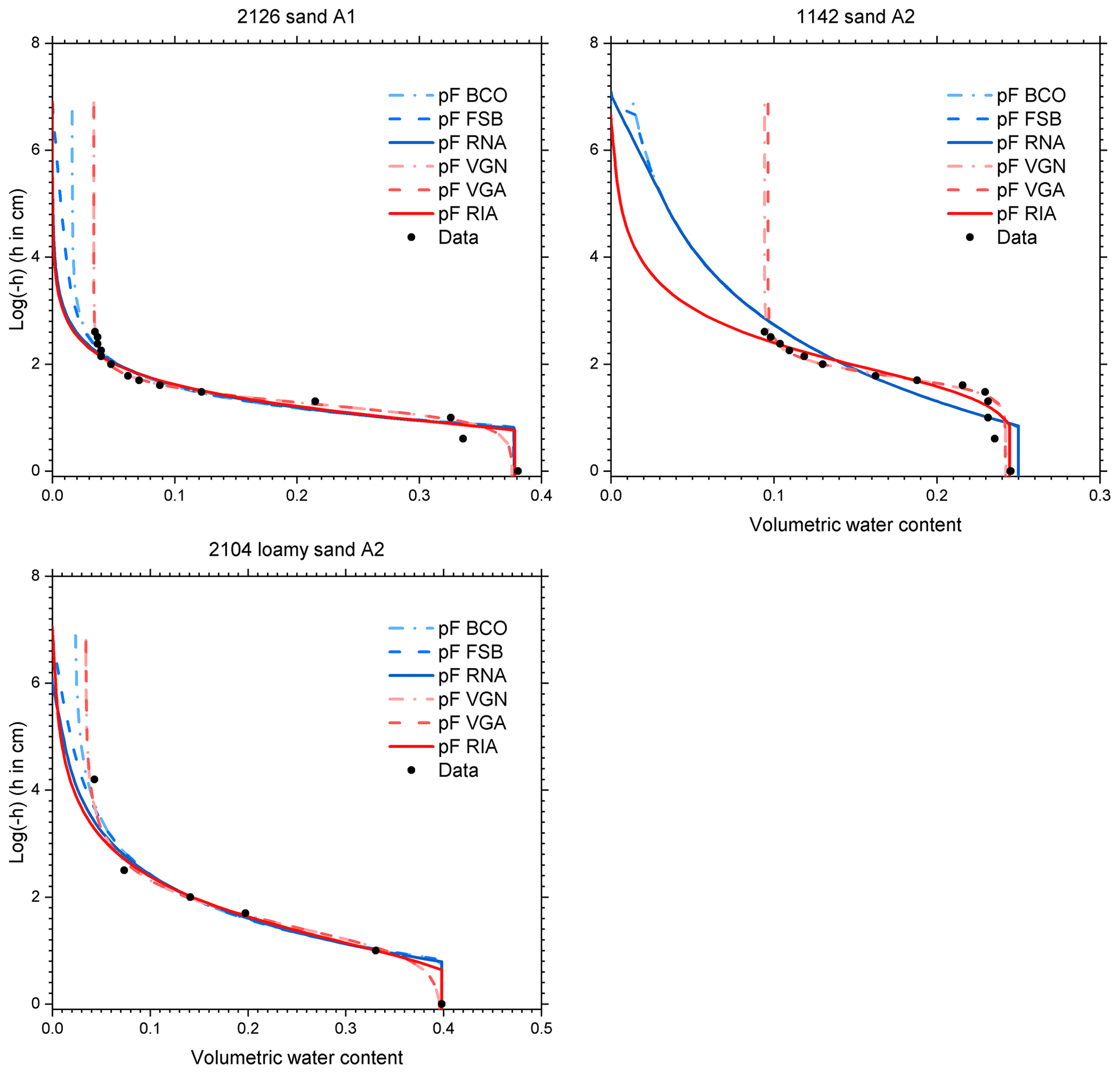
Figure C2 Retention data and fitted soil water retention curves according to six parameterizations for selected UNSODA soils with the A1 or A2 classification of Twarakavi et al. (2010). The parameterizations are explained in the text.

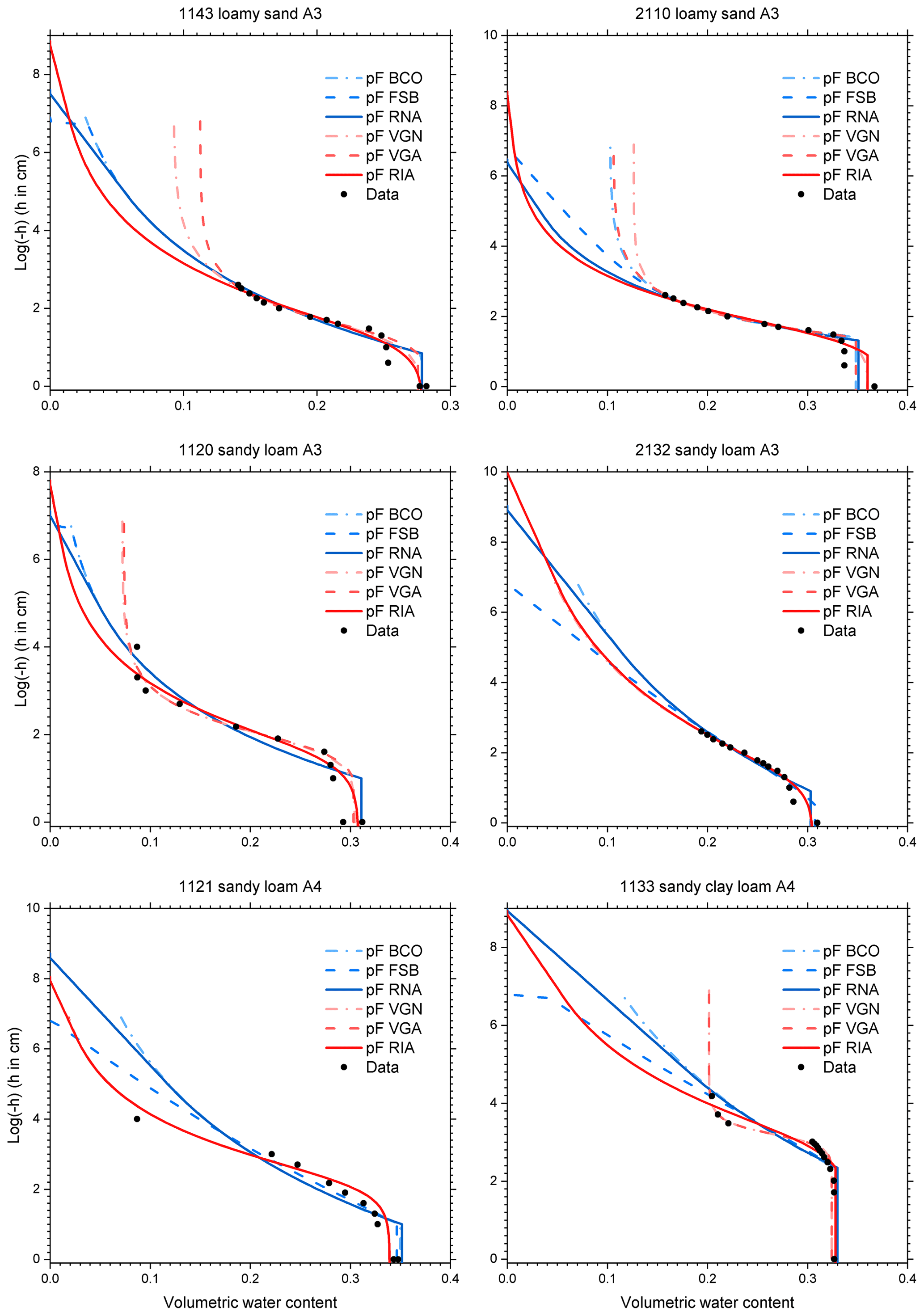
Figure C3 Retention data and fitted soil water retention curves according to six parameterizations for selected UNSODA soils with the A3 or A4 classification of Twarakavi et al. (2010). The parameterizations are explained in the text.

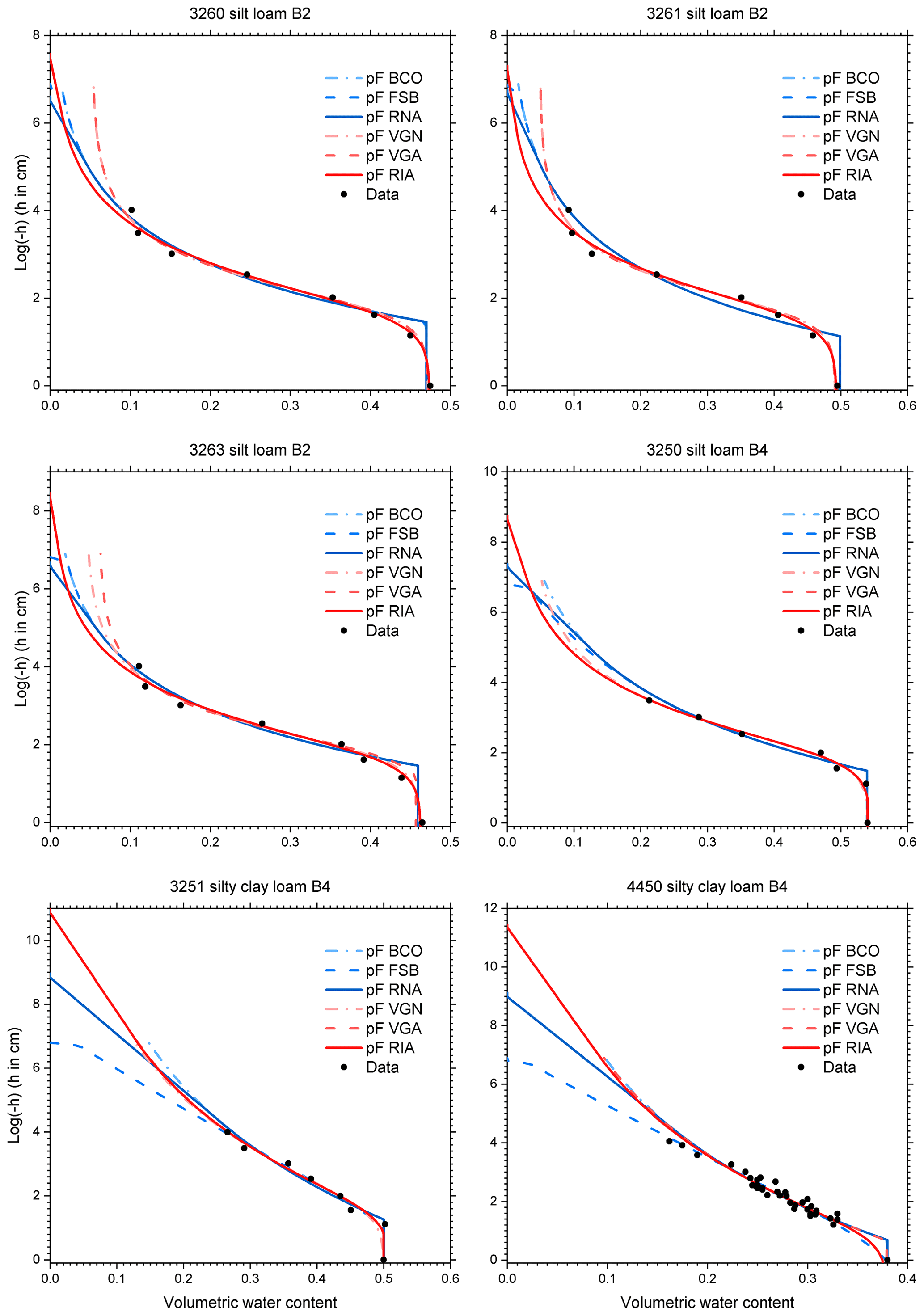
Figure C4 Retention data and fitted soil water retention curves according to six parameterizations for selected UNSODA soils with the B2 or B4 classification of Twarakavi et al. (2010). The parameterizations are explained in the text.

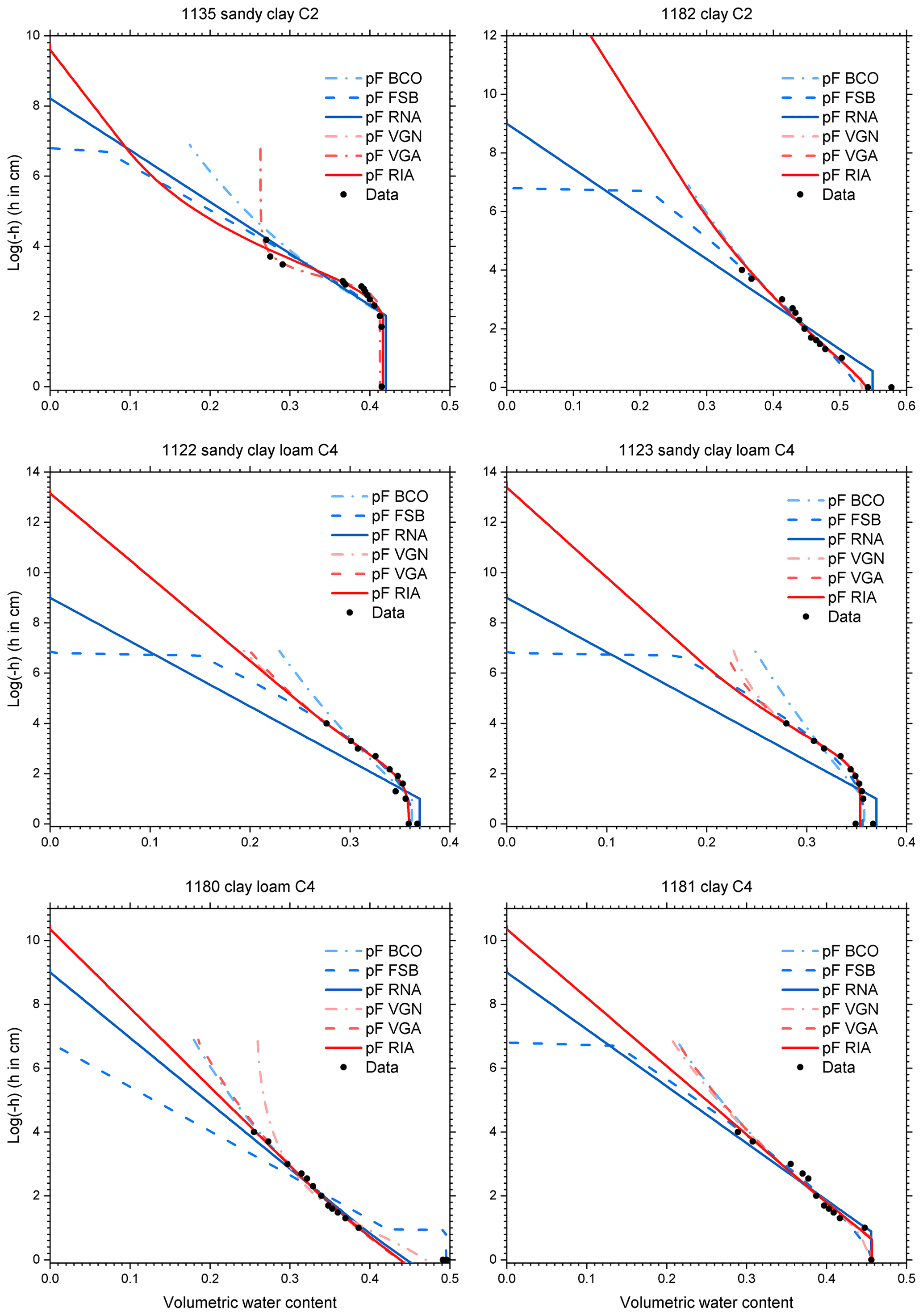
Figure C5 Retention data and fitted soil water retention curves according to six parameterizations for selected UNSODA soils with the C2 or C4 classification of Twarakavi et al. (2010). The parameterizations are explained in the text.

Figure C6 Conductivity data and conductivity curves derived from the retention curves of Fig. C2, according to six parameterizations for selected UNSODA soils with the A1 or A2 classification of Twarakavi et al. (2010).

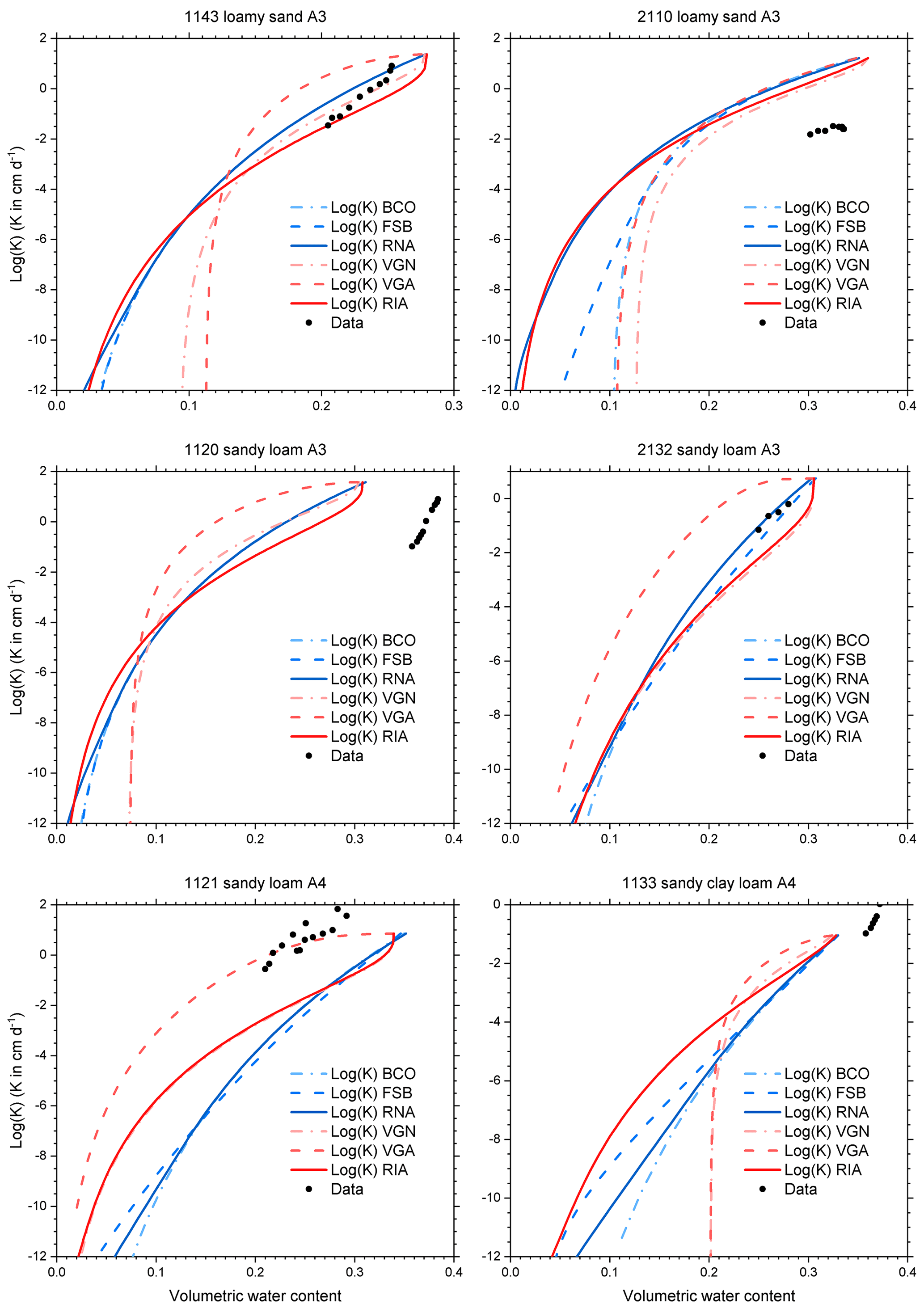
Figure C7 Conductivity data and conductivity curves derived from the retention curves of Fig. C3, according to six parameterizations for selected UNSODA soils with the A3 or A4 classification of Twarakavi et al. (2010)

Figure C8 Conductivity data and conductivity curves derived from the retention curves of Fig. C4, according to six parameterizations for selected UNSODA soils with the B2 or B4 classification of Twarakavi et al. (2010).

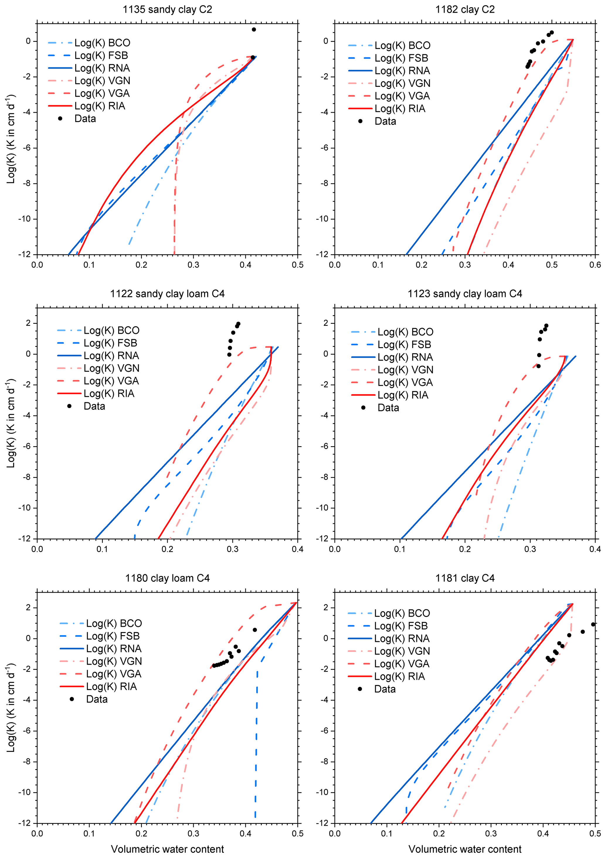
Figure C9 Conductivity data and conductivity curves derived from the retention curves of Fig. C5, according to six parameterizations for selected UNSODA soils with the C2 or C4 classification of Twarakavi et al. (2010).

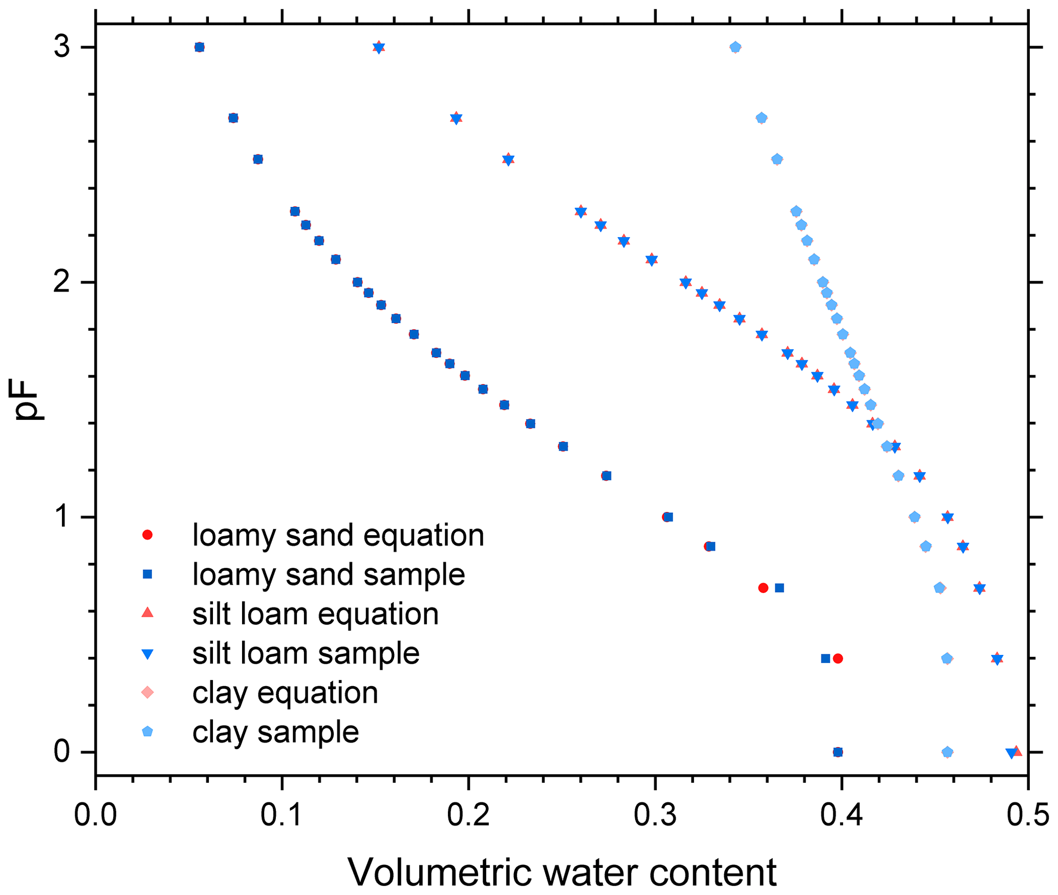
Figure C10 Soil water retention points calculated from RIA parameterizations for loamy sand (UNSODA identifier 2104, classified according to Twarakavi et al., 2010; A4), silt loam (3261; B2), and clay (1181; C4). The points were either calculated directly for the given pF value (“equation”), or by calculating the average water content in a sample of 5.0 cm height at hydrostatic equilibrium, with the matric potential at the centre of the sample corresponding to the indicated pF value (“sample”). Note: the data points for zero matric potential were plotted at pF = 0 instead of pF = −∞.

The SWRCs defined by these parameterizations, together with the data points on which they are based, are given in Figs. C2–C5. The hydraulic conductivity curves that, according to Mualem (1976), can be derived from the parameterizations (Eqs. 14a and 14b for RIA; equations for the other parameterizations in Madi et al., 2018) are plotted in Figs. C6–C9. We plotted K as a function of θ because this relationship is less hysteretic than K(h) (Koorevaar et al., 1983, p. 141), and some of the UNSODA data only provided K(θ) data points. The conductivity data available in UNSODA are also plotted, but these were not used to fit the curves. The maximum pF value for which points on the curves were calculated was set at 6.8 for VGN and VGA and to the pF value corresponding to the fitted value of h_d for RIA.

The comparison of theoretical conductivity curves, based on water retention data with the measured values, showed a sometimes substantial deviation between hydraulic conductivities measured at saturation, and the K_s value used to create the theoretical curves. The latter value was obtained by a query that made the database return a K_s value for the soils that met all other criteria also included in the query. The conductivity data displayed in the plots were separately obtained by requesting that the database return a report of tabular data for each of the 21 soils. The reasons for the discrepancies between the queried value and the tabulated data may reflect separate experiments for measuring unsaturated and saturated values of K.

There also are obvious differences between the water content at saturation between the retention and the conductivity data. In all but one case (soil 4450; Fig. C8), the hydraulic conductivity observations were made in the field whereas the retention data used were all obtained from drying experiments in the laboratory. Scale differences, the effects of air enclosure and hysteresis in the field, and differences between different measurement techniques explain these differences. We can, therefore, only compare the shape of the theoretical curves with those of the data clouds.

The RMSE was calculated from the weighted sum of squares of the differences between calculated and observed water contents and pressure heads. The weights equaled the estimated scaled standard deviations (SDs) of the individual water retention observations (pairs of matric potential and water content values). The SDs of the water content observations were scaled to have an average value of 0.2. The scale factor needed to arrive at this value was then applied to the SDs of the matric potential values as well. This ensured that the weighting of the water contents and matric potential values was consistent with the original SDs of both. The scaling greatly improved the efficiency of the parameter-fitting procedure. The squared difference between a single observed water content and its fitted value during a given iteration of the parameter-fitting algorithm, taking into account observation errors in both the water content and the matric potential, is as follows:

$$\begin{array}{}\text{(C1)}& {\left({\displaystyle \frac{{\mathit{\theta }}_{\text{fit}}-{\mathit{\theta }}_{\text{obs}}}{{\mathit{\sigma }}_{\mathit{\theta },\text{scaled}}+{\mathit{\sigma }}_{h,\text{scaled}}\frac{\mathrm{d}\mathit{\theta }}{\mathrm{d}h}{\mathrm{|}}_{h_{\text{obs}}}}}\right)}^{\mathrm{2}},\end{array}$$

where σ_a,scaled is the scaled SD of the variable a, the subscript “fit” signifies a fitted value of the subscripted variable, and the subscript “obs” is a measured value (Madi et al., 2018). The slope of the SWRC in the denominator is estimated from the fitted parameterization using the parameter values that have been fitted in the iteration that is currently being tested.

The scale factors applied to the observation error SDs varied between soils but not between parameterizations fitted to the same soil. RMSE values of different parameterizations valid for a particular soil can therefore be readily compared. Comparisons between soils only give a rough indication. When the water contents at which measurements were taken differ strongly from one soil to another, then the comparison of their RMSE values is less reliable.

In case the measured water contents were obtained at hydrostatic equilibrium, the fitted water content calculated directly from the matric potential could not be compared to the observed water content. To approximate the soil sample on which the observation was made, a hypothetical soil slab of the same height as the sample was divided into 20 horizontal layers. If UNSODA did not specify the sample height, it was assumed to be 5.0 cm. The matric potential in the centre of each layer was determined from the given matric potential, which was assumed to apply to the centre of the sample. The water content of the soil slab was then calculated as the average water content of its 20 layers. This water content was used to calculate the difference between the observed and the fitted water content. Figure C10 shows a comparison of the retention points calculated for three soils, based directly on the RIA parameterization and based on the same parameterization applied to a hypothetical sample of 5.0 cm height at hydrostatic equilibrium, with the nominal matric potential valid at the sample centre. Deviations are small, even for the loamy sand.