Assessing different imaging velocimetry techniques to measure shallow runoff velocities during rain events using an urban drainage physical model

Although surface velocities are key in the calibration of physically based urban drainage models, the shallow water depths developed during non-extreme precipitation and the potential risks during flood events limit the availability of this type of data in urban catchments. In this context, imaging velocimetry techniques are being investigated as suitable non-intrusive methods to estimate runoff velocities, when the possible influence of rain has yet to be analyzed. This study carried out a comparative assessment of different seeded and unseeded imaging velocimetry techniques based on large-scale particle image velocimetry (LSPIV) and bubble image velocimetry (BIV) through six realistic but laboratory-controlled experiments, in which the runoff generated by three different rain intensities was recorded. First, the use of naturally generated bubbles and water shadows and glares as tracers allows unseeded techniques to measure extremely shallow flows. However, these techniques are more affected by raindrop impacts, which even lead to erroneous velocities in the case of high rain intensities. At the same time, better results were obtained for high intensities and in complex flows with techniques that use artificial particles. Finally, the study highlights the potential of these imaging techniques for measuring surface velocities in real field applications as well as the importance of considering rain properties to interpret and assess the results obtained. The robustness of the techniques for real-life applications yet remains to be proven by means of further studies in non-controlled environments.

1 Introduction

Since the last years of the 19th century, urban drainage systems have fulfilled a fundamental mission that has enabled us to guarantee the hygienic-sanitary conditions and growth of denser cities (Butler et al., 2018; Brown et al., 2009). However, today several factors are threatening the sustainability and flood response capacity of urban drainage systems. The increment in impervious areas, due to urbanization (Shuster et al., 2005; Yao et al., 2016) and ongoing climate change, among other factors, is resulting in a higher and more frequent number of heavy rainfall events (Willems et al., 2012; Arnbjerg-Nielsen et al., 2013). The increased flood risk is a consequence of these factors (Chen et al., 2015) that must be accurately assessed (Apel et al., 2004; Martinez-Gomariz et al., 2016). This continuous development of impervious areas also leads to a significant increase in the load and peak concentrations of pollutants, which are accumulated on urban catchments surfaces and can be washed off and transported by runoff into drainage systems and eventually to aquatic media (Lee and Bank, 2000; Anta et al., 2006; Zafra et al., 2017; Muthusamy et al., 2018). This process depends on multiple factors (Hatt et al., 2004; García et al., 2017) and requires a clear understanding of the surface drainage in urban areas, from the hydrodynamic point of view.

In this context, physically based urban drainage models can help to assess complex cases, such as the definition of the inlet capacity of different storm drains to transfer runoff stormwater into sewers (Martins et al., 2018; Rubinato et al., 2018) or to assess particle wash-off processes (Hong et al., 2016; Naves et al., 2020a). Calibrating these models requires precise characterization of the surface velocities and flow depth, due to their key role in flood risk assessment and in the detachment and transport of surface pollutants. However, punctual velocity measurement equipment such as acoustic Doppler velocimetry (ADV) does not enable a two-dimensional velocity field to be obtained in large urban areas during flood events without a huge deployment of instrumentation and a major risk to workers. Furthermore, due to the shallow runoff flows during non-extreme events, ADV reliability is reduced as it is an intrusive technique that also needs about 5–7 cm to obtain velocity measurements (Cea et al., 2007). Imaging techniques are becoming more widely used in open and large-scale environments as non-intrusive methods for the characterization of surface velocity fields (Aberle et al., 2017) and are becoming increasingly common for river monitoring (e.g., Tauro et al., 2016, 2018; Manfreda et al., 2018; Pearce et al., 2020). Large-scale particle image velocimetry (LSPIV) is an image velocimetry technique that provides velocity fields in large areas, even in the proximity of hydraulic structures (Muste et al., 2008; Fujita et al., 1998; Kantoush et al., 2011). LSPIV velocity determination can be affected by deficient illumination, diffuse light reflections, or free-surface waviness generated by wind or large-scale turbulence structures. Seeding is also a key parameter of the technique that may need to be artificially improved (Aberle et al., 2017). Zhu et al. (2019) achieved errors below 14 % using this technique in a full-scale stormwater detention basin, although in some boundary points the error could reach 44 %.

In addition, LSPIV-based methods can be applied to determine runoff velocities without the presence of particles, such as in Leitão et al. (2018), in which a method called surface structure image velocimetry (SSIV; Lüthi et al., 2014; Hansen et al., 2017) introduces some improvements based on image preprocessing analysis to measure shallow flows in a flood experimental facility. In addition, bubbles are used as tracers to estimate overland velocities in the technique known as bubble imaging velocimetry (BIV). The BIV technique was first introduced to measure the velocity field in high aerated flows from backlit image analysis without the need for laser-like illumination (Ryu et al., 2005). Bubbly flows are illuminated by a uniform light source, while a high-speed camera captures shadow textures created by gas–liquid interfaces (Aberle et al., 2017). Lin et al. (2012) have already used this technique to measure the flow structure in hydraulic jumps in the aerated zone.

In Naves et al. (2019a), a variation of the LSPIV technique was applied to measure the surface velocity fields generated by three different rain intensities in a full-scale urban drainage physical model. The presence of raindrops in the experiments can generate disturbances in the water surface and also interfere in the visualization of images, so that the study used UV illumination and fluorescent particles as artificial tracers to satisfactorily address those issues. To the best of the authors' knowledge, that was the first and only study in which an imaging velocimetry technique has been applied during rainy conditions. Despite the proposed methodology's good results and its great suitability for laboratory applications, its transferability to field studies is restricted by the difficulties in using artificial particles and special illumination. However, in addition to the interferences mentioned above, the raindrop impacts also generate bubbles and some other structures on free-flow surfaces that may be used as tracers in unseeded techniques. Due to the great potential of these unseeded techniques to obtain overland flow velocity data in field applications using, for example, pre-installed surveillance cameras (Leitão et al., 2018), studying their performance under rainy conditions is an interesting and novel research gap to be addressed.

Therefore, experimental videos of the overland flow generated by three different rain intensities, under laboratory-controlled conditions and recorded with and without artificial particles, are used in this study to comparatively assess the performance of different seeded and unseeded imaging velocimetry techniques under rainy conditions. First, the sensitivity of the velocity results to the analysis parameters is investigated in order to test the robustness of each method. Then, the resulting velocity fields are compared to analyze the feasibility of using each visualization technique in different characteristic flows developed in urban catchments and to investigate the influence of rain intensity in velocity measurements as the novel contribution. The LSPIV procedure, already validated in Naves et al. (2019a), is used as the reference technique in this analysis. Finally, the potential of these imaging techniques to measure runoff velocities in real field applications is discussed.

2 Materials and methods

The experimental work performed to record the overland shallow flows generated by three different simulated rainfall events in an urban drainage physical model is introduced first, in Sect. 2.1. Then, Sect. 2.2 includes a description of the procedure followed to obtain velocity results from the original video frames. Section 2.3 describes the strategy to assess the performance of different image velocimetry techniques depending on rain intensity and the typology of flow. Finally, the surface areas on which the analysis was focused, the ranges of variation of the parameters involved in the assessment of the robustness of each technique, and the procedure implementation details are explained in detail in Sect. 2.4, 2.5, and 2.6.

2.1 Experimental data

The freely available experimental dataset (Naves et al., 2019b) described in Naves et al. (2020b) was used in this study for the assessment of different imaging velocimetry techniques. The dataset comprises a series of videos in which the surface runoff was recorded in a 36 m² urban drainage physical model. The facility (Fig. 1a) consists of a full-scale street section in which the rainfall runoff generated by a dripper-based rainfall simulator, which is able to produce three different rain intensities (30, 50, and 80 mm h⁻¹), drains into a pipe system through two gully pots. The roughness value of the roadway concrete surface is 0.016 (Naves et al., 2019a). Two types of configurations have been used to visualize overland flow: (a) experiments using fluorescent particles and UV illumination and (b) experiments using white-LED lamps without artificial particles to highlight air bubbles and water reflections generated by raindrops in the flow. While seeded videos were already used in the application of a modified LSPIV technique in Naves et al. (2019a) as stated in the introduction section, unseeded videos are used for the first time in this work to consider imaging velocimetry techniques that do not require artificial tracers. Figure 1b shows a scheme of the configuration of the experiments in which the videos were recorded.

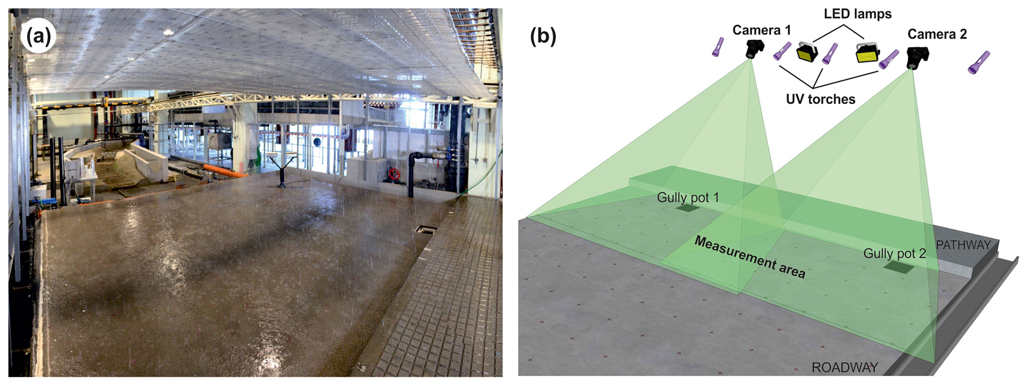
Figure 1 General image of the urban drainage physical model with the rainfall simulator (a) and experimental setup of the PIV experiments (b).

As seen in Fig. 1b, two Lumix GH4 cameras with 28 mm focal length recorded the first 2 m attached to the curb along 5 m of the physical model. UV torches and LED lamps were installed next to the cameras 2.2 m above the pathway. During the experiments, videos were recorded at 4 K resolution and 25 Hz. A total of 1500 frames of steady flow (equivalent to 60 s) were then extracted from the longer recording and processed for analysis. To do this, frames were scaled and ortho-rectified using the known 2D coordinates of 28 and 24 reference surface points for each camera and the MATLAB functions “fitgeotrans” and “imwarp”. Finally, the reference points placed in the intersection between the recorded areas of each camera were used to crop and join the image, resulting in raw images in which 1 pixel corresponds to 1 mm in real-world coordinates. Examples of these images obtained from UV seeded and LED unseeded experiments, which are openly available for others to use in the dataset published by the authors (Naves et al., 2019b), are included in Fig. 2. These six sets of images considering both the experimental setup and the three rain intensities were used as the basis for the different imaging velocimetry techniques assessed in this study. A more detailed description of the physical model, the simulated rain, and the procedure to extract the images can be consulted in Naves et al. (2020b, c, 2019a), respectively.

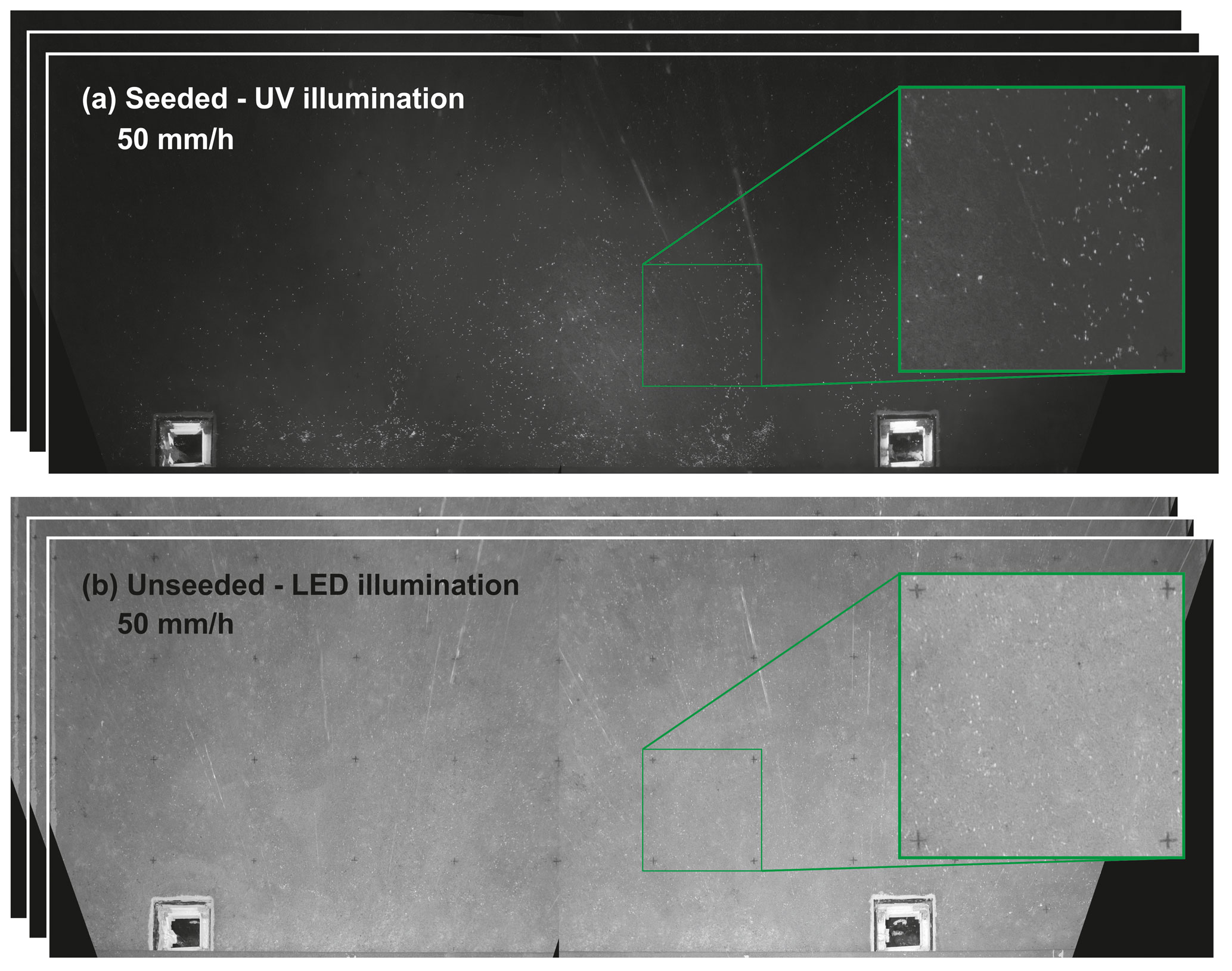
Figure 2 Example of frames used for the assessment of different imaging velocimetry techniques. Images correspond to the two experiments performed for the rain intensity of 50 mm h⁻¹, using fluorescent particles and UV illumination (a) and using led lamps to highlight water reflections and air bubbles present in the flow (b).

2.2 Analysis procedure and imaging velocimetry techniques

Four imaging velocimetry techniques were considered in this study to estimate overland flow velocities. First, the LSPIV methodology was assessed using the images with fluorescent particles and UV illumination. This methodology requires preprocessing of images through a sliding background (SLB), which eliminates the background of the images and particles that remain immobile between frames. These particles, which are deposited due to the extreme low depths developed and the roughness of the concrete surface, should be removed to avoid the null velocities resulting from them conditioning the particle image velocimetry (PIV) analysis. Then, a LSPIV-based method, named LSPIVu in this work, and the BIV technique were used to obtain velocity fields from the unseeded and LED-illuminated experiments. LSPIVu is inspired by the non-open SSIV procedure employed in Leitão et al. (2018) and uses SLB image preprocessing to remove the background from the analysis and satisfactorily trace the movement of air bubbles and surface water reflections generated by raindrops. Additionally, BIV implements a previous binarization of the grayscale images to highlight bubbles from a determined threshold. Finally, a slight variation of the LSPIV methodology named LSPIVb was implemented to investigate the influence of binarization also in the analysis of seeded UV experiments. This strategy seeks to isolate the brightest pixels, which in this case correspond with the fluorescence particles, to ensure that other elements such as bubbles or water reflections do not interfere in the PIV analysis. Therefore, the image velocimetry techniques differ in the preprocessing of the images and the experiments used for the analysis. A diagram of the procedure followed for each technique is presented in Fig. 3, which includes a common PIV cross-correlation analysis and a post-processing of the velocity results. The different image velocimetry techniques and the steps of the analysis are further explained below.

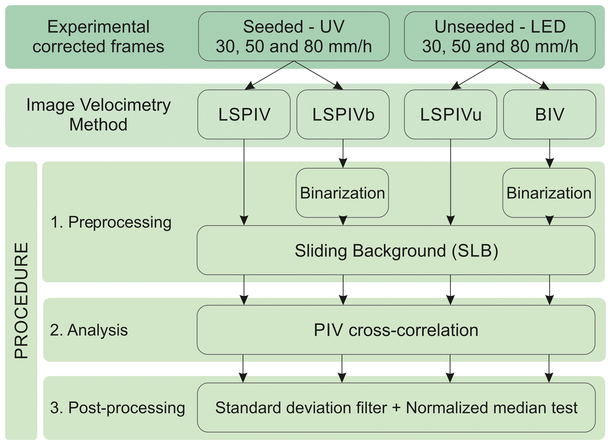
Figure 3 Diagram of the procedure performed to obtain velocity fields from video frames for the different image velocimetry techniques.

2.2.1 Preprocessing

As seen in Fig. 3, the first step in the analysis procedure was the preprocessing of the images depending on the technique employed. The objective of this part of the analysis was to optimize the input images through different strategies to enhance the objective tracers and then measure their movement with PIV algorithms in the next step. The specific procedure followed for each technique is now described.

LSPIV velocity determination was undertaken using the experimental videos with fluorescent tracers and UV illumination as in Naves et al. (2019a). The preprocessing in the implementation of this method consists of a sliding background filter. This filter compares the gray values of the pixels of one frame with the same pixels of the following one, turning those pixels with a certain percentage of agreement between them to black. Therefore, it is necessary to determine a certain threshold of similitude to remove the background of the images and the particles that stay still between frames whilst keeping those that are transported by flow. Thus, it is possible to avoid interferences in the cross-correlation of the particle movement that may reduce the mean velocity obtained.

In the case of the LSPIVb procedure, a binarization of the images was performed in the image preprocessing, prior to applying the sliding background filter. This converts the grayscale images to binary images, turning the pixels with gray values greater than a certain threshold to white and all other pixels to black. This filter ensures that only the fluorescent particles are considered in the PIV cross-correlation, preventing possible small interferences that bubbles or water reflections may produce despite the special illumination (Zhou et al., 2013). Due to this binarization, the subsequent sliding background filter is applied considering a threshold of 100 % of similitude to remove the pixel, so only the binarization threshold should be adjusted.

In contrast to LSPIV and LSPIVb, the LSPIVu technique was applied to the images taken from the unseeded and LED illuminated experiments. LSPIVu is analogous to the LSPIV procedure, applying the sliding background filter below a certain threshold to remove the background of the original images. In this technique, the preprocessing of the images seeks to analyze the movement of both surface air bubbles and water reflections generated by raindrops. Lastly, the procedure of the BIV technique additionally includes an image binarization filter, as was used in the LSPIVb methodology, to isolate air bubbles to be used as tracers in the analysis of the images taken from the unseeded experiments.

2.2.2 PIV cross-correlation

The different alternatives of image processing, depending on the image velocimetry technique (LSPIV, LSPIVb, LSPIVu or BIV), were applied to 60 s of images taken in steady flow conditions, and the resulting frames were then analyzed by the PIV image software PIVLab (Thielicke and Stamhuis, 2014). This software performs a cross-correlation analysis between consecutive frames, which are divided into different interrogation areas (IAs), to obtain the mean displacement vector for each of the IAs. The size of the IA is a parameter that must be adjusted as a function of the mean displacement in order to achieve suitable results. Common procedures to estimate this particle displacement, and thus flow velocity, have been applied in the present work (Raffel et al., 2007; Adrian et al., 2011). The discrete Fourier transform (DFT), calculated using a fast Fourier transform (FFT), was used to compute the correlation matrix in the frequency domain. Moreover, two passes of a multi-pass window deformation algorithm were used, halving the window size at the second pass to achieve a higher spatial resolution. The searching area (SA) matches the IA, and 50 % of overlapping was selected in all cases. These procedures are included in most of the conventional PIV algorithms such as PIVLab (Thieckle and Stamihus 2014) or OpenPIV (Taylor et al., 2010).

2.2.3 Post-processing

Two filters for the detection of spurious vectors were applied to the velocity fields obtained. First, the results were filtered to remove those velocity vectors that differed by 4 times the standard deviation of the mean velocity of the individual velocity fields. Then, the normalized median test was applied in a 3×3 neighborhood as proposed in Westerweel and Scarano (2005). After preliminary tests assessing the performance detecting spurious vectors in the PIV results, the values of the two parameters of this filter were set at ε=0.15 and threshold = 3. Outliers and missing data were removed and not replaced in any case. The average velocity field was obtained from the 1500 velocity results in steady conditions obtained for each case of study, which makes them comparable to the results achieved in Naves et al. (2019a) using the LSPIV technique. In this study, the velocities were compared as measured from the movement of tracers without applying velocity indexes to estimate depth-averaged velocities.

2.3 Comparative evaluation of image velocimetry methods

The repetitiveness of the experiments has allowed for the evaluation of techniques that require different experimental setups varying the seeding and illumination. First, following the specific procedure explained in the previous section (Sect. 2.2) for each technique, the analysis started with the individual assessment of the robustness of the velocity results achieved by each technique. This assessment was carried out in a manner similar to Legout et al. (2012). The key parameters of the procedure were varied one at a time within reasonable ranges to investigate their influence on the average velocity results. The parameters considered were (a) the preprocessing parameter, which corresponds with the sliding background or the binarization threshold depending on the image velocimetry technique; (b) the IA initial size in the cross-correlation algorithm; and (c) the frame acquisition rate (FAR) of the experimental videos. The entire analysis was focused on four areas of the model surface in order to separately consider different types of flow that are developed in real catchments.

Moreover, a detailed comparison of the mean velocity fields achieved from 1 min of steady conditions using each technique was performed considering each of the three rain intensities and each of the four surface areas and using the LSPIV method as reference. Finally, the transferability of the previous imaging velocimetry techniques to field studies is discussed considering the previous results and an additional convergence analysis, which assesses the uncertainties involved in measuring velocities in transient conditions. Further details of the studied areas, the ranges of the parameters, and the implementation methodology are included in Sect. 2.4, 2.5, and 2.6.

2.4 Areas considered for analysis

The urban drainage physical model considered in this study enables typical flows such as those that are developed in real catchments to be reproduced. Figure 4 includes the previous velocity field results obtained in Naves et al. (2019a) for the rain intensity of 50 mm h⁻¹ and the drainage basin of gully pot 2. As can be observed, the runoff generated by the rainfall simulator produces two perpendicular flows: a very shallow flow towards the curb and a longitudinal curb flow with depths of up to 10 mm that drains the runoff into the gully pots. In addition, some preferential drainage channels, where velocities are significantly increased, have been detected in the overland flow perpendicular to the curb due to irregularities in the model surface.

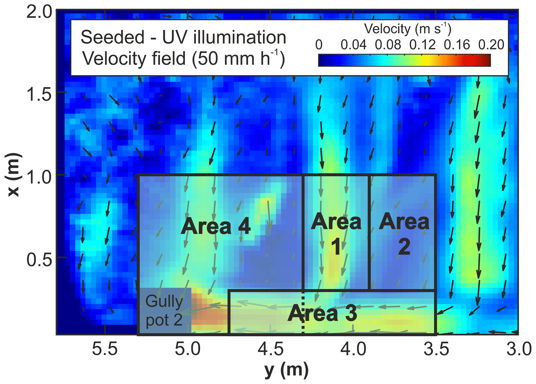
Figure 4 Areas of the model surface analyzed with the image velocimetry methods considering different types of flows that are developed in urban catchments: perpendicular drainage to the curb (Areas 1 and 2), curb flow (Area 3), and vicinities of gully pot 2 (Area 4). The velocity field plotted to understand the choice of the analyzed areas was taken from Naves et al. (2019a), in which the LSPIV was satisfactorily applied.

The comparative analysis performed in this study was focused on four specific areas of the model surface in order to assess the performance of the techniques considered for different types of water flows that may be found in real catchments. These are straight overland flow in one main direction as presented in Area 1, where a preferential channel with high velocities is distinguished; a parallel overland flow out of the main drainage channels with very low velocities and water depths (Area 2); the curb flow gathering different secondary flows with a vertical boundary (Area 3); and a combination of the previous type of flows in the vicinity of gully pot 2 (Area 4). Figure 4 includes the specific position in the model surface of each area considered in the analysis performed.

2.5 Parameters ranges

As stated in Sect. 2.3, the first part of the analysis performed seeks to assess the robustness of the velocity results and their sensitivity to changes in the different input parameters of the procedure, depending on the image velocimetry technique used. The base parameters established in the analysis and their ranges of variation are given in Table 1. First, the FAR of the videos taken from the experiments was 25 Hz, which was established as the reference value since it is typical of most imaging devices available on the market. Furthermore, one of two and one of three consecutive images were extracted to analyze a FAR of 12.5 and 6.25 Hz, respectively. This simulates the FAR of some already installed devices, such as traffic or surveillance cameras, that may serve as a media source to measure urban runoff velocities in field applications as per the ideas stated in Leitão et al. (2018).

Table 1 Ranges of the parameters considered in the analysis of the different image velocimetry methods. Values in parentheses specify the base value of the parameters used as reference.

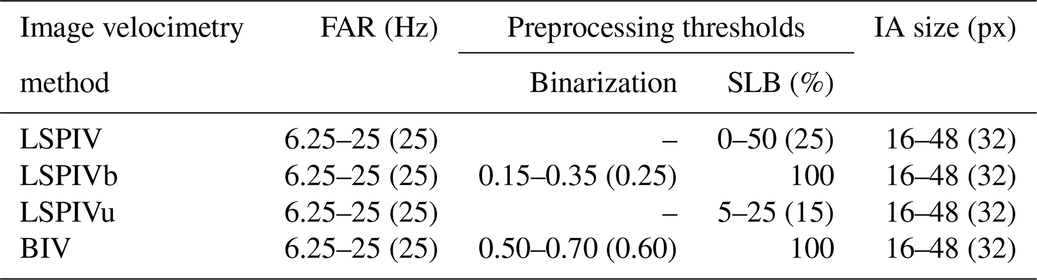
The variations produced in the velocities because of changes in the preprocessing parameters were also investigated. In the cases of LSPIV and LSPIVu, only the sliding background threshold was considered since binarization was not performed. In contrast, LSPIVb and BIV required the definition of the binarization threshold, but the sliding background threshold had to be fixed at 100 % to delete those pixels that appear in white in two consecutive and binarized frames. The reference value of these thresholds and their range of variation during the analysis were determined based on expertise and preliminary tests. This resulted in variations of the SLB threshold from 0 % to 50 % for LSPIV and from 5 % to 25 % for LSPIVu and binarization thresholds from 0.15 to 0.35 for LSPIVb and from 0.50 to 0.70 for BIV. Reference values were thus established as the mean value for each range.

The reference value for the IA size during the cross-correlation process was set following the recommendations in Raffel et al. (2007) and Adrian et al. (2011). As the maximum velocity vectors are around 10 pixels per frame in absolute values, the reference interrogation area (IA) is set at 32×32 pixels. This ensures the rule of thumb that displacements cover around 25 % of the total size of the IA. The range of IA sizes was established within 16 and 48 pixels.

2.6 Implementation

The variations of the velocity results because of changes in the parameters were analyzed by varying the reference value of one determined parameter within its established range. In addition to the reference value, four different values were also considered using uniform steps for the IA size and the preprocessing parameter. For example, IA sizes of 16, 24, 32, 40, and 48 pixels were investigated, whilst the remaining parameters were kept constant. As commented in Sect. 2.5, the FAR has been modified between 25, 12.5, and 6.25 Hz. This resulted in 11 different parameter sets for each of the four different image techniques, three different rainfall events, and four different areas. Therefore, a total of 528 cases were considered when analyzing the 1500 raw frames recorded in the seeded or unseeded experiments. The representation of velocity fields was performed through the MATLAB toolbox “pivmat” (Moisy, 2017).

3 Results and discussion

In the present section, the differences obtained in the velocity fields resulting from analyzing the experimental videos by four image velocimetry techniques (LSPIV, LSPIVb, LSPIVu and BIV) are presented and discussed. First, the sensitivity of the different methods to image processing variables is investigated to assess their robustness and performance in analyzing shallow flows with the presence of raindrops. Then, velocity results are compared, and the feasibility of using these techniques in transient flow conditions is analyzed.

3.1 Sensitivity to image processing analysis

The changes in the mean velocities obtained by varying the key parameters of the analysis for the three study areas, the four imaging velocimetry techniques, and the rain intensity of 50 mm h⁻¹ are shown in Fig. 5. The graph includes velocity results as the average of the mean velocities resulting from each pair of frames analyzed (1500 in the case of the frequency acquisition rate of 25 Hz), plotting their standard deviation using whiskers. The reference value and the range of variation of the parameters considered, which are the preprocessing parameter (binary threshold or sliding background depending on the technique used), the interrogation area size (IA), and the frequency acquisition rate (FAR), were previously defined in Sect. 2.5. This analysis focused on the intermediate rain intensity experiments. Results for 30 and 80 mm h⁻¹ experiments are similar and can be consulted in the Supplement. Generally speaking, Fig. 5 shows how varying the parameters within the established ranges did not produce significant variations in the mean velocity results. Therefore, the methodology and the imaging velocimetry techniques analyzed in this work are presented as being robust, and the reference values can be considered when comparing the velocity results obtained by each technique.

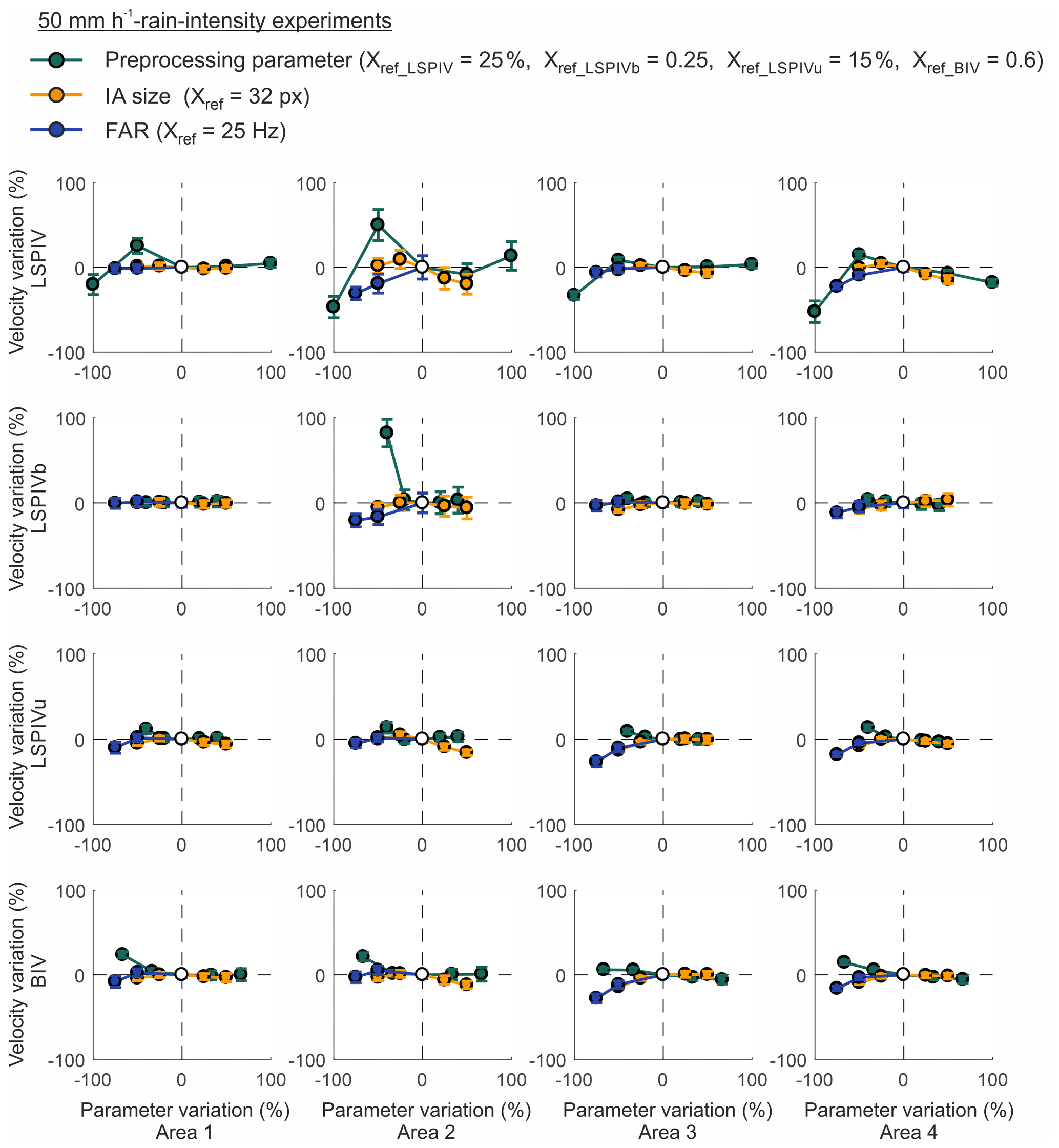
Figure 5 Percentage of variation in the mean velocities when varying parameters of the analysis for the four studied areas (columns) and the four imaging velocimetry techniques considered (rows) in the case of 50 mm h⁻¹ rainfall. Mean velocity variability for the different pairs of frames analyzed is included using whiskers.

Considering techniques that use seeded experiments (LSPIV and LSPIVb), the preprocessing parameter showed the greatest influence on the results. This is due to the importance of removing particles that remain still on the model surface in order to achieve reliable results. As seen in the results, the binarization considered in LSPIVb reduces this sensitivity to the preprocessing parameter, except in Area 2 where the extremely shallow flow considered greatly favors particle deposition. The very low depths developed in this area also increase the variability of the mean velocities depending on the pair of frames analyzed, which remains low for the rest of the cases, as can be seen from the plotted whiskers. The techniques that analyze the videos without particles (LSPIVu and BIV) are slightly less sensitive to variations in the parameters. In summary, the results obtained by the imaging velocimetry techniques are presented as being quite stable, and the velocities do not depend on the parameters being within reasonable ranges established by expertise. Therefore, the velocity results obtained from the reference parameter values are representative of each technique and can thus be used to assess their performance. Finally, an expected degradation was noted when FAR is reduced but within assumable ranges that make it possible to consider cameras with lower FAR as a media source for field applications.

3.2 Velocity results' comparison

The performance of each technique was assessed by comparing the velocity field results obtained in the study areas by each technique for the three rain intensities considered. Following the previous results (Sect. 3.1), the reference values of the parameters (Table 1) have been considered for this comparison. Additionally, the LSPIV technique was used as the reference since it had been previously validated in Naves et al. (2019a). The comparative results are presented below for each study area to analyze in detail the performance of each technique for the different types of flow developed on the model surface.

First, Fig. 6 shows the comparison of the velocity fields in Area 1, which corresponds to a main drainage channel perpendicular to the curb where high velocities are developed. The velocity fields obtained and a derived disparity plot using the LSPIV results as the reference are included in Fig. 6 for the three different rain intensities. The first aspect to highlight is that the implementation of binarization in the preprocessing of the frames introduced no significant improvements in the velocity field results. In contrast, very important differences were observed by comparing techniques that analyze videos with (LSPIV and LSPIVb) and without (LSPIVu and BIV) particles. All visualization techniques presented a similar velocity distribution for the lowest rain intensity (first row), although an offset of approximately 0.05 m s⁻¹ was obtained for the unseeded techniques. This offset occurred because the different tracers used in seeded and unseeded experiments are affected by raindrop impacts to different degrees and may be transported at different velocities. When considering the novel application of these techniques in the presence of rain, one can deduce that all techniques obtained a good performance for 30 mm h⁻¹ rainfall. It can be further stated that, in the case of unseeded techniques, lower velocity indexes are required in order to convert the results to depth-averaged velocities, as observed in previous references (Leitão et al., 2018; Martins et al., 2018; Naves et al., 2019a). However, the velocity fields obtained for rain intensities of 50 and 80 mm h⁻¹ showed that both the LSPIVu and the BIV technique resulted in erroneous velocity distributions, with those areas being more affected where greater velocities are developed. In the case of the rain intensity of 50 mm h⁻¹, there is an unexpected reduction in velocities for the unseeded techniques, which is greatly incremented as the velocities are higher than roughly 0.10 m s⁻¹ for the LSPIV technique. With regard to the 80 mm h⁻¹ results, it can be deduced that this issue in measuring velocities is clearly related with the rain intensity, since the perturbations in the velocity results started to occur for lower LSPIV velocities and to a greater extent as the rain intensity increased.

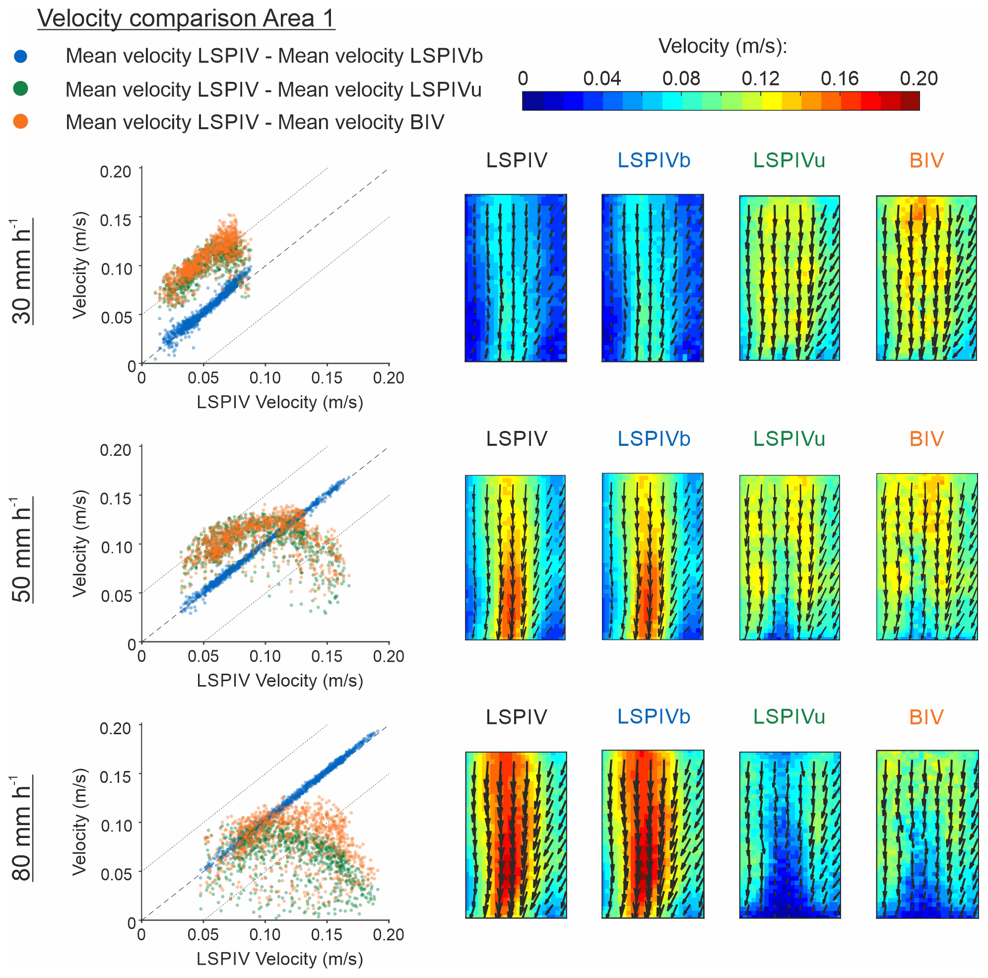
Figure 6 Velocity comparison between imaging velocimetry techniques results (LSPIV, LSPIVb, LSPIVu, and BIV) in Area 1 for the three different rain intensities (30, 50, and 80 mm h⁻¹). The velocity fields obtained for each case are also plotted for a qualitative comparison.

This phenomenon can be explained by the combination of two different processes. First, the reduction in the gap between velocities obtained from the seeded and unseeded techniques for LSPIV velocities lower than 0.10 m s⁻¹ is due to the turbulence generated by the raindrop impacts, which decrease the flow surface velocity. The velocity index to estimate depth-averaged velocities therefore depends on the rain intensity. Then, the problems of unseeded techniques (LSPIVu and BIV) measuring velocities with high rain intensities do not arise because of a lack of tracers since, as can be observed in the videos provided in Naves et al. (2019b), the number of bubbles in that area increases with the rain intensity. These are caused by the erratic trajectory of the bubbles observed in the unseeded videos for high rain intensities, due to the impact of raindrops on the water surface. It is assumed that raindrops, when falling, interrupt part of the existing flow and produce acceleration of the flow in all directions in the area surrounding the impact (Kilinc and Richardson, 1973). The natural bubbles used as tracers for the LSPIVu and BIV techniques are highly affected by such accelerations, producing very fast, random, and major changes in the position of the tracers; this phenomenon is exacerbated as the velocity of the bubbles and the rain intensity increase. This prevents cross-correlation algorithms from obtaining displacements of tracers and results in erroneous velocities. The mass of the fluorescent particles used as tracers in the case of LSPIV and LSPIVb, with a density slightly higher than water, gives them inertia to avoid such sudden movements and to allow for cross-correlation between consecutive frames.

Despite these problems in measuring velocities with high rain intensities, the use of bubbles as tracers in low rain intensities can provide an opportunity to measure velocities in extremely shallow flows where the particles tend to be deposited, as can be seen on the sides of the drainage channel in the velocity fields of Fig. 6. This is better assessed in the analysis of the results in Area 2 (Fig. 7), which is attached to Area 1 and considers a flow perpendicular to the curb, out of the main drainage channels and where very shallow flows are developed.

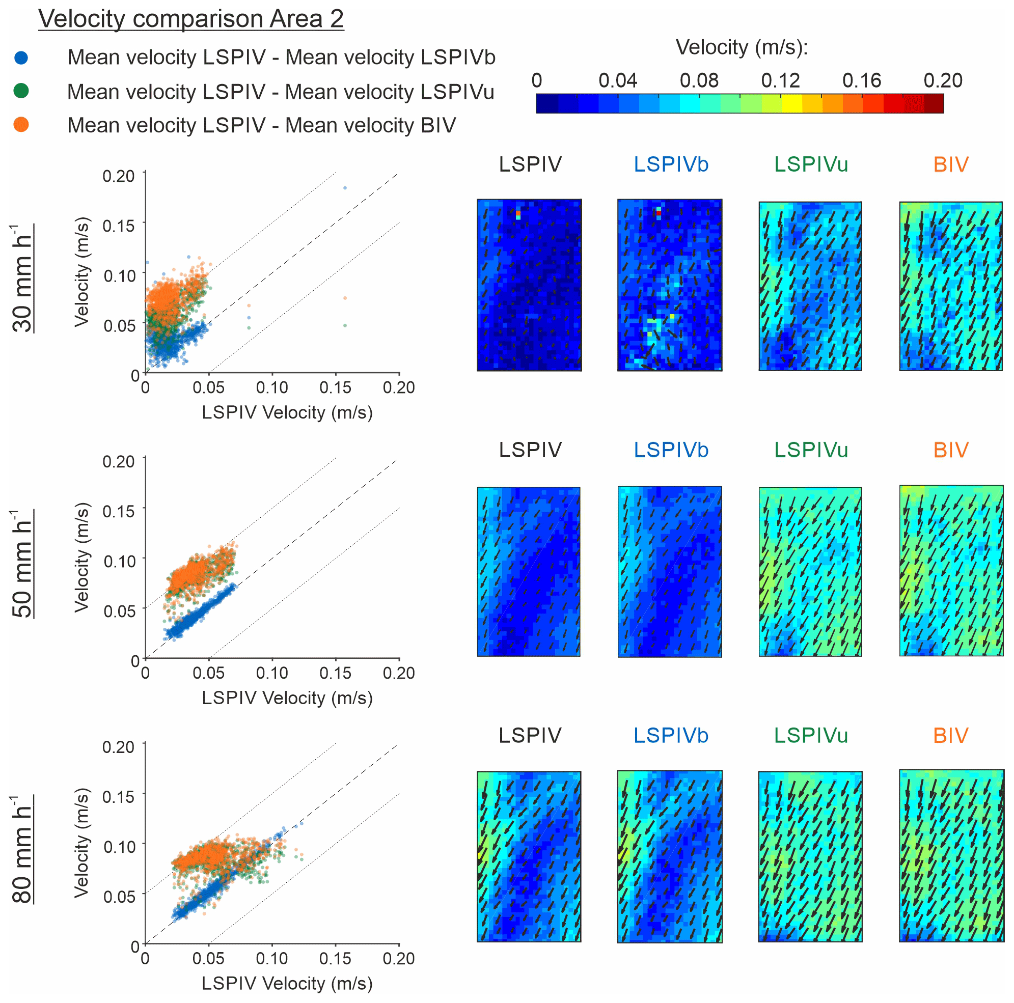
Figure 7 Velocity comparison between imaging velocimetry techniques results (LSPIV, LSPIVb, LSPIVu, and BIV) in Area 2 for the three different rain intensities (30, 50, and 80 mm h⁻¹). The velocity fields obtained for each case are also plotted for a qualitative comparison.

As can be seen in Fig. 7, there is a central zone in Area 2 where the methods that use particles as tracers (LSPIV and LSPIVb) are not able to obtain velocity data (dark blue areas in the respective velocity fields). In this zone, which corresponds to the lowest water depths and becomes smaller as the rain intensity is higher and the water depths increase, the LSPIVu or BIV techniques need to be used to obtain reliable results. This is because bubbles can pass through the extremely shallow areas where fluorescent particles tend to be deposited, which can be checked in the recorded videos. Regarding the influence of the rain intensity on the results, a similar behavior to that for Area 1 is observed, but in this case, only the experiment with the highest rain intensities results in erroneous velocities, due to the low velocities recorded.

Figure 8 presents the comparison between the velocity results in Area 3. The velocity fields in this area refer to the channel attached to the curb that runs perpendicular to the flows presented in Areas 1 and 2 and where most of the overland flows are gathered on their way to the drain inlet. Figure 8 only includes velocity fields for the rain intensity of 50 mm h⁻¹, since no interesting differences were found between rain intensities; the rest of the velocity field can be consulted in the Supplement. In the recorded videos of the unseeded experiments, it was observed that raindrop impacts do not produce bubbles in that area due to the greater water depths. Moreover, existing bubbles cannot access that flow from the rest of the catchment and therefore stay retained in the confluence of flows. This results in a lack of tracers and thus the impossibility of measuring velocities correctly with the LSPIVu and BIV techniques. In contrast, LSPIV and LSPIVb present a high density of particles and accurate velocity results with a high concordance between both techniques. Therefore, it can be concluded that measuring velocities in those conditions is not possible using the LSPIVu technique to trace water reflections without the presence of bubbles, so the use of particles as tracers is highly recommendable in this type of complex flow.

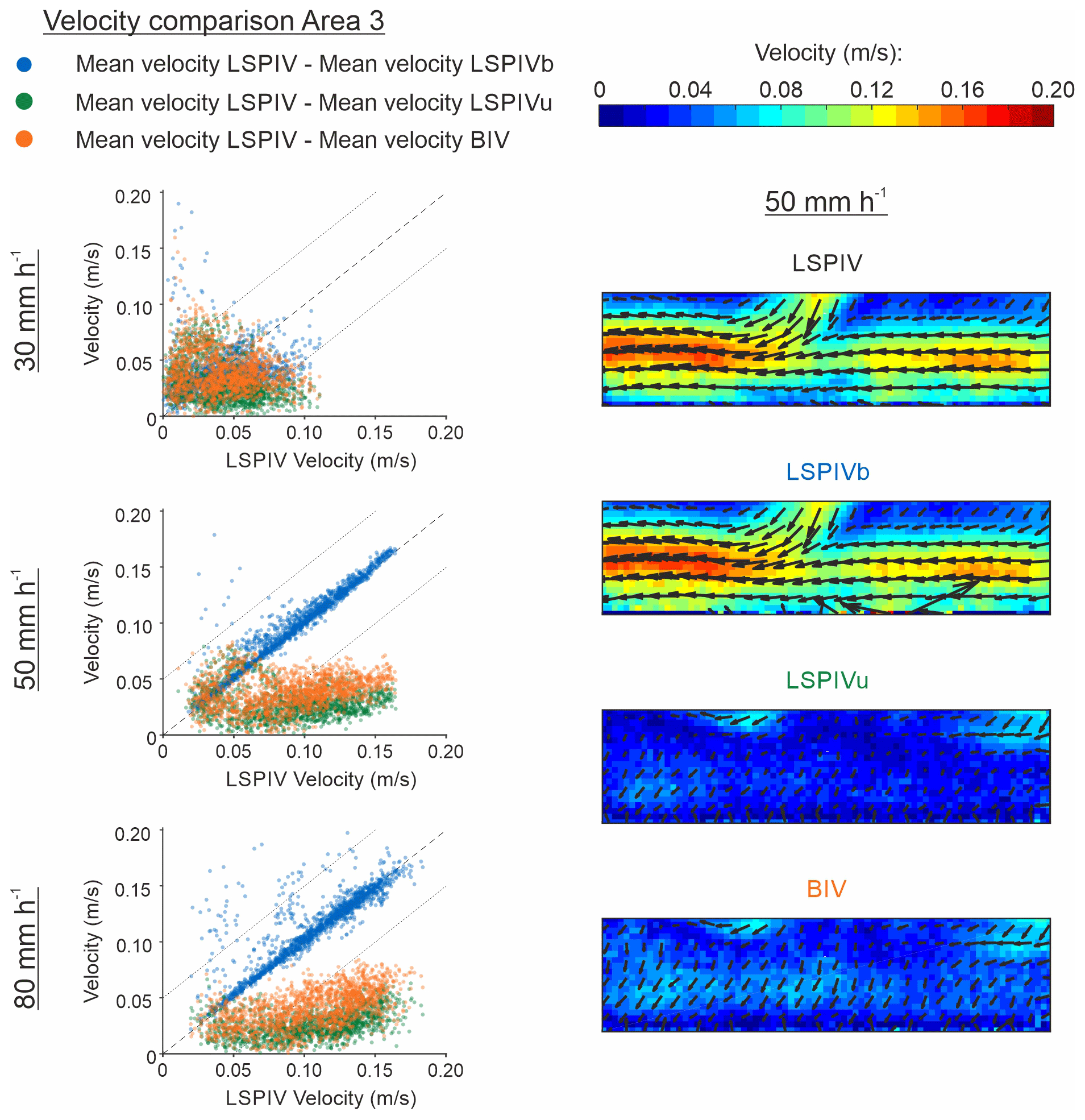
Figure 8 Velocity comparison between imaging velocimetry techniques results (LSPIV, LSPIVb, LSPIVu, and BIV) in Area 3 for the three different rain intensities (30, 50, and 80 mm h⁻¹). The velocity fields obtained for the case of 50 mm h⁻¹ are also plotted for a qualitative comparison.

Finally, Fig. 9 shows the velocity fields obtained in Area 4 for the case of 50 mm h⁻¹ and the comparison between the results obtained using the four imaging velocimetry techniques and the three rain intensities. The velocity fields for rain intensities of 30 and 80 mm h⁻¹ can be consulted in the Supplement. Area 4 covers the vicinity of gully pot 2 and is a combination of the previous cases studied considering overland flows perpendicular to the curb, such as those in Areas 1 and 2 and the curb flow analyzed in Area 3. The results plotted in Fig. 9 agree with the observations made for the previous areas and confirm the insights achieved.

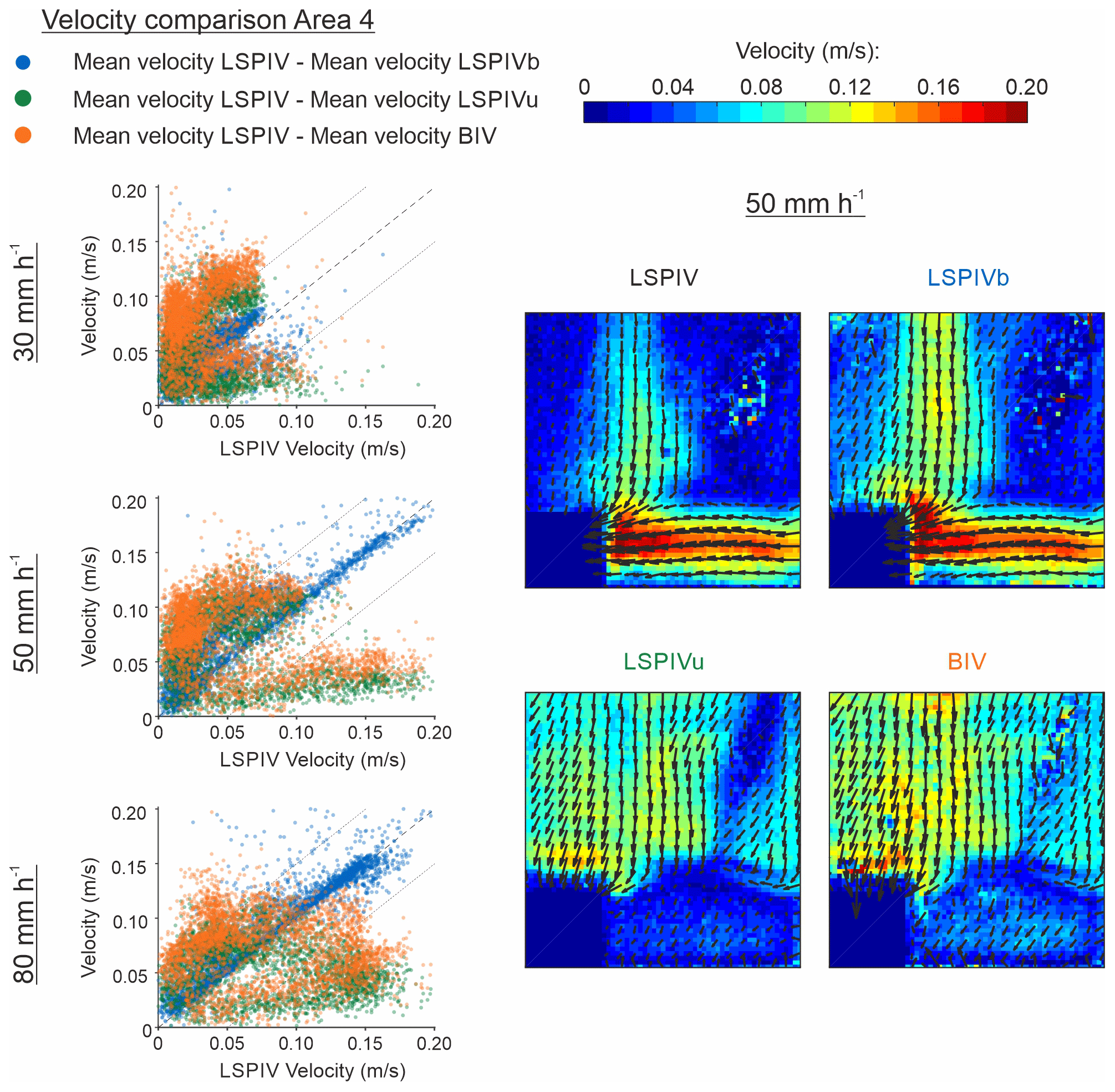
Figure 9 Velocity comparison between imaging velocimetry techniques results (LSPIV, LSPIVb, LSPIVu, and BIV) in Area 4 for the three different rain intensities (30, 50, and 80 mm h⁻¹). The velocity fields obtained for the 50 mm h⁻¹ case are also plotted for a qualitative comparison.

As seen in Naves et al. (2019a), LSPIV gave suitable results for the entire model surface, with some difficulties in extremely shallow flows with depths of around 1 mm where particles tend to be deposited. Then, the velocity fields showed very similar results between LSPIV and LSPIVb and between LSPIVu and BIV, with slightly higher velocities measured by methods using binarization preprocessing (LSPIVb and BIV). This similarity indicates that, except for particles and bubbles, the cameras did not record many other moving elements that disturb the results, so binarization does not include significant benefits in those experiments. In addition, it was observed that techniques that include binarization result in noisier velocity results (see velocity fields for 30 and 80 mm h⁻¹ in the Supplement). This may be because, if binarization is applied, the sliding background filter may remove parts of tracers in motion that are overlapped in consecutive frames since no different gray values are considered. This might also explain the slightly higher velocities obtained. Therefore, this filter should be used with care in future applications if it is necessary to isolate tracers from other mobile elements. In the case of the lowest rain intensity, all the techniques gave similar velocity distributions with the offset of around 0.05 m s⁻¹ observed in the previous areas between the seeded and unseeded techniques, which is due to the different tracers analyzed. The use of bubbles as tracers gives unseeded techniques the opportunity to measure velocities in extremely shallow flows where particles tend to be deposited. However, LSPIVu and BIV are more affected by the impact of raindrops, thus leading to erroneous results for high rain intensities, especially for high velocity flows. These techniques also presented problems in the flow attached to the curb because of the absence of bubbles in that area.

3.3 Transferability to field applications

The assessment of different imaging velocimetry techniques and the analysis of the influence of different factors on the velocity results contribute to understanding how these methodologies could be adequately transferred to real urban catchments. The use of these techniques would favor new velocity data sources to calibrate physically based urban drainage models, such as traffic, public, or surveillance cameras (Leitão et al., 2018; de Vitry et al., 2020) or even unmanned aerial vehicles, which have already been used in river flow measurements (e.g., Lewis and Rhoads, 2018; Pearce et al., 2020). The insights gained in this study show the limitations of unseeded LSPIVu and BIV techniques to estimate runoff velocities under high rain intensity conditions or when complex flows are developed. Raindrop impacts on the water surface produce disturbances in the movement of the bubbles used as tracers that can prevent cross-correlation algorithms from obtaining reliable velocity distributions. In our experiments, this problem was observed when the rain intensity was higher than 30 mm h⁻¹, but this threshold may vary depending on the overland flow velocity or the raindrop kinetic energy. However, as there is no need to add artificial particles in the unseeded techniques, they benefit from being straightforward to implement. Their ability to estimate velocities in extremely shallow flows, where particles tend to be deposited, also makes these techniques a potential tool for measuring velocities in field applications without the interference of raindrops or under light rain conditions. In contrast, it was observed that using artificial particles as tracers makes the LSPIV and LSPIVb techniques robust against heavy rain conditions and complex flows, such as those developed in Area 3 of the present study (Fig. 8). Therefore, the use of seeded techniques is recommended to estimate overland velocities in real urban catchments under rainy conditions or when the measured flows are not simple enough. Special attention must be paid to the deposition of particles when the flow is extremely shallow.

Besides the ability of each technique to adequately measure overland flow velocities in urban catchments with shallow water flows and the presence of raindrops, it is important to determine the minimum requirements of the recording devices when evaluating the potential of using these techniques in field studies. This work has demonstrated that a low-frequency acquisition rate of 6.25 Hz could be used, incorporating acceptable errors into the velocity results obtained. However, in light of the problems observed in Leitão et al. (2018) for rates lower than 20 Hz using only water reflections as tracers, this requirement varies according to the magnitude of the measured velocities and the tracer used. Therefore, it is deduced that artificial particles and naturally generated bubbles considered in the present study favor cross-correlation when the time step between frames is increased. The outdoor study carried out by Leitão et al. (2018) also concluded that an LSPIV-based method provides robust results, analyzing images with a resolution as low as 256×144 pixels for an area of around 5 m². These values are easily overcome by most imaging devices available on the market, so, although low acquisition rates and image resolution will decrease the precision and quality of the velocity results, they do not represent a major constraint to transferring imaging velocity techniques to real applications in urban catchments.

Finally, the analysis presented in this article has been performed for steady flows comparing average velocity fields obtained from 1 min of steady conditions. This enables the results to be compared with those obtained in Naves et al. (2019a) and reduces the uncertainties in velocity estimations but is not representative of field conditions. Therefore, another important point to address concerns the uncertainties assumed when using these techniques in transient flows, such as those that would be recorded in real catchments. A convergence analysis is presented in Fig. 10 for the experiments with 50 mm h⁻¹ rain intensity and for Areas 1, 2, and 3, showing the variations in the mean velocities that arise when the number of frames considered is reduced. The first result to highlight is that the mean velocities obtained from each method and from each area follow the insights presented and discussed in Sect. 3.2. In addition, the variations in the mean velocity remain low when considering 25 frames in the analysis, which corresponds to 1 s in the present case study. This value is considered to be enough to ensure reliable velocity results when analyzing transient flows and to enhance the possible usability of these imaging velocimetry techniques in future real field studies, meriting further investigation. Convergence results for other rain intensities and for Area 4 are similar and can be consulted in the Supplement.

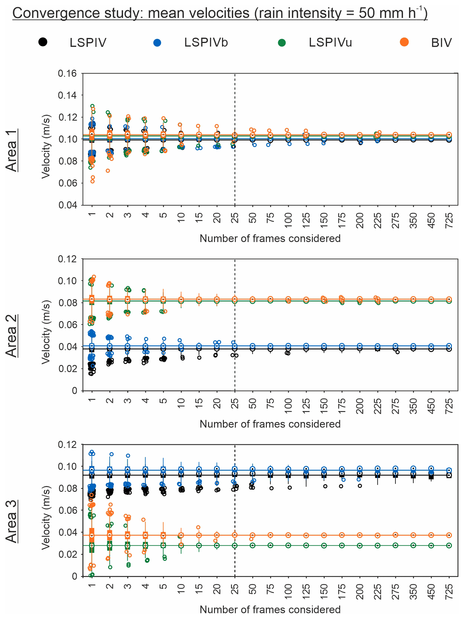
Figure 10 Mean velocity convergence study for rain intensity of 50 mm h⁻¹ and Areas 1, 2, and 3. The horizontal line represents the mean velocity considering all the frames available (1500) for LSPIV (black), LSPIVb (blue), LSPIVu (green), and BIV (orange) techniques. Then, the variability in the mean velocity when the frames are divided into groups of different numbers of frames is represented by box plots.

4 Conclusions

In this study, the performance of different seeded and unseeded imaging velocimetry techniques has been assessed from videos of the overland flow generated by three different rain intensities in an urban drainage physical model. These techniques use artificial seeded particles or existing bubbles and water reflections as tracers to estimate surface velocity distributions. The influence of the rain intensity on the reliability of the results has also been explored as a novel scientific contribution by comparing the velocity fields achieved from each study case. Based on the results obtained, the following conclusions can be drawn:

• The variation in the parameters of the imaging velocimetry techniques within the established ranges did not produce significant variations in mean velocity results. Therefore, the methodology and the imaging velocimetry techniques analyzed in this work are presented as being robust, and expertise can be used to set the required parameters for the analysis.

• Both the seeded and unseeded techniques provide suitable velocity distributions in cases of unidirectional flows and the lowest rain intensity of 30 mm h⁻¹, with an offset of approximately 0.05 m s⁻¹ between them. This offset is a consequence of the different tracers used in the seeded and unseeded experiments, which are affected to different degrees by raindrop impacts and may be transported at different velocities. Lower velocity indexes are thus required in the case of unseeded techniques to convert the results to depth-averaged velocities, and these are affected by rain intensity.

• LSPIVu and BIV unseeded techniques are not able to estimate runoff velocities for higher rain intensities due to the disturbances introduced by raindrop impacts, which prevent cross-correlation algorithms from obtaining displacements and thus velocity distributions. The use of artificial particles as tracers by LSPIV and LSPIVb makes these seeded techniques robust against heavy rain conditions, and they are thus recommended in future field studies during rain events. Seeded techniques are also able to measure complex flows, where bubbles have difficulties in following the overland flow, avoiding unseeded techniques to determine velocities. However, unseeded techniques can be suitable in field and laboratory applications in unidirectional flows and without the interference of raindrops or under light rain conditions, since they require a simpler experimental setup and are able to measure velocities in extremely shallow waters where artificial particles tend to be deposited.

• The similarity found between LSPIV and LSPIVb and between LSPIVu and BIV indicates that binarization preprocessing has no significant benefits in these experiments as the cameras did not record moving elements that significantly disturb the results. In addition, it has been found that this procedure leads to noisier results, so binarization should be used with care in future applications if it is necessary to isolate tracers from other mobile elements.

• The rapid convergence of velocity results makes the analysis of transient flows feasible. This fact, as well as the not very demanding requirements of the recorded videos, favors the transferability of these techniques to field studies, where they can be used as a novel tool to obtain runoff velocities in order to calibrate physically based urban drainage models.

This work evaluated the reliability of different imaging techniques obtaining urban runoff velocities in different types of flows and with the presence of raindrops, highlighting the importance of considering rain properties to interpret and assess the results obtained by these techniques. The potential use of seeded and unseeded techniques in urban catchments has been proven, but future research should be oriented towards studying their robustness in real-world applications under non-controlled environments. The influence of the wind on rainfall distribution, catchment surface roughness, or variable illumination conditions should be assessed in order to develop suitable preprocessing and post-processing procedures and correctly estimate runoff velocity results.