In-stream Escherichia coli modeling using high-temporal-resolution data with deep learning and process-based models

Contamination of surface waters with microbiological pollutants is a major concern to public health. Although long-term and high-frequency Escherichia coli (E. coli) monitoring can help prevent diseases from fecal pathogenic microorganisms, such monitoring is time-consuming and expensive. Process-driven models are an alternative means for estimating concentrations of fecal pathogens. However, process-based modeling still has limitations in improving the model accuracy because of the complexity of relationships among hydrological and environmental variables. With the rise of data availability and computation power, the use of data-driven models is increasing. In this study, we simulated fate and transport of E. coli in a 0.6 km² tropical headwater catchment located in the Lao People's Democratic Republic (Lao PDR) using a deep-learning model and a process-based model. The deep learning model was built using the long short-term memory (LSTM) methodology, whereas the process-based model was constructed using the Hydrological Simulation Program–FORTRAN (HSPF). First, we calibrated both models for surface as well as for subsurface flow. Then, we simulated the E. coli transport with 6 min time steps with both the HSPF and LSTM models. The LSTM provided accurate results for surface and subsurface flow with 0.51 and 0.64 of the Nash–Sutcliffe efficiency (NSE) values, respectively. In contrast, the NSE values yielded by the HSPF were −0.7 and 0.59 for surface and subsurface flow. The simulated E. coli concentrations from LSTM provided the NSE of 0.35, whereas the HSPF gave an unacceptable performance with an NSE value of −3.01 due to the limitations of HSPF in capturing the dynamics of E. coli with land-use change. The simulated E. coli concentration showed the rise and drop patterns corresponding to annual changes in land use. This study showcases the application of deep-learning-based models as an efficient alternative to process-based models for E. coli fate and transport simulation at the catchment scale.

1 Introduction

Contamination of surface waters through microbiological pollutants is a major public health concern (Bain et al., 2014). Worldwide, pathogens tend to wreak havoc on human health because of the diseases they cause, such as diarrhea, resulting in infant mortality. In particular, developing countries are vulnerable to pathogen-related diseases due to the deficit of sanitation facilities (Boithias et al., 2016). Escherichia coli (E. coli) has been frequently used as an indicator of fecal bacteria because it is easy to culture (Rochelle-Newall et al., 2015). Higher concentrations of E. coli in water tend to be linked to fecal pathogenic microorganisms, harmful to human health. Although long-term and high-frequency E. coli monitoring can help prevent waterborne diseases from fecal pathogenic microorganisms, monitoring E. coli concentrations is time-consuming and expensive (Cho et al., 2016; Frolich et al., 2017; Kim et al., 2017). Furthermore, high-frequency datasets of E. coli concentration are scarce, and available long-term datasets are often inadequate to yield a continuous time series of fecal pathogenic microorganisms (van der Leeuw, 2004). Modeling approaches can overcome this drawback in monitoring. Thus, they can be a means to determine the fate and transport of fecal pathogenic microorganisms at the catchment scale by simulating E. coli in environmental compartments, such as the soil surface and streams (Ligaray et al., 2016; Pachepsky and Shelton, 2011).

Several process-based models have been developed to simulate stream water contamination by E. coli. Popular models to simulate E. coli are the Soil and Water Assessment Tool (SWAT) (Neitsch et al., 2011), Hydrological Simulation Program–FORTRAN (HSPF) (Bicknell et al., 1997), INCA-Pathogens (Whitehead et al., 2016), and pathogen catchment budget (PCB) (Ferguson et al., 2007). The fate and transport of E. coli are a complex phenomenon with several drivers (Pachepsky et al., 2018), such as the hydrological regime (Boithias et al., 2016; Pachepsky et al., 2017), contributions of both surface runoff and subsurface flow to the overall in-stream discharge (Boithias et al., 2021b), concentration and sources of suspended sediment (Ribolzi et al., 2016; Nguyen et al., 2016), land use (Causse et al., 2015; Nakhle et al., 2021), intrinsic properties of the bacterium (Pachepsky et al., 2014), and economic conditions (Iqbal et al., 2019). Recently, Sowah et al. (2020) applied the SWAT model to research the sources and drivers of E. coli in the Clouds Creek watershed, USA. However, the process-based models still have limitations to accuracy due to the complexity of relationships among hydrological and environmental variables (Abimbola et al., 2020). In addition, the simplified equations of these models can increase the inherent uncertainties, resulting in simulation errors. To overcome these limitations, several modifications of the E. coli module of the SWAT model have been proposed to incorporate the impacts of the multiple drivers of E. coli fate and transport (Kim et al., 2018; Meshesha et al., 2020). The E. coli concentration in surface water varies significantly within a very short time period (Chen et al., 2014; Boithias et al., 2021b). Daily simulations cannot capture the dynamics of E. coli in a short duration. In particular, the simulation with high temporal resolution is important in small headwater catchments because the duration of flood events might be less than 1 d (Gassman et al., 2007). Therefore, an E. coli concentration simulation with high temporal resolution should be conducted to determine the temporal distribution of E. coli.

Recently, deep learning (DL) has become a promising alternative approach for estimating water quality by using features of water constituent dynamics (Pyo et al., 2021). Deep-learning-based models are superior to their process-based counterparts due to their high accuracy, faster prediction time, and ability to model complex physical phenomena (Sze et al., 2017). Deep-learning models can exploit a particular compositionality in the input features by finding more abstract features in them (Bengio et al., 2021). Long short-term memory (LSTM) networks have an advantage over other deep-learning-based models in that they can extract complex patterns from sequence data (Schmidthuber and Hochreiter, 1997). Several studies have applied deep learning to water quality modeling and prediction (Peterson et al., 2020; Isikdogan et al., 2017; Solanki et al., 2015). Dong et al. (2019) used LSTM to predict dissolved oxygen concentrations and showed that LSTM performs better than other machine-learning methods, such as autoregressive integrated moving average or artificial neural networks. Although LSTM has been used extensively for building hydrological models (Abbas et al., 2020), its potential has not yet been explored to estimate E. coli concentration in stream waters. Deep-learning-based models have also not been developed for the simulation of water quality with high temporal resolution.

This study aims to evaluate the applicability of LSTM to simulate in-stream E. coli concentrations with high temporal resolution. In addition, the process-based model HSPF was used as a benchmark to compare and assess the performance of LSTM. Both models were applied to a 0.6 km² tropical headwater catchment from the northern Lao People's Democratic Republic (PDR). The temporal resolution of the simulations was 6 min in both models. Thus, the specific objectives of this study were to compare the performance of a process-based model and a deep-learning model (1) to simulate both surface and subsurface flow, (2) to simulate E. coli concentration, and (3) to analyze the response of E. coli to changing land use.

2 Materials and methods

2.1 Study site and data acquisition

The study area is the 0.6 km² Houay Pano headwater catchment, located 10 km south of the city of Luang Prabang, Lao PDR (Boithias et al., 2021a) (Fig. 1). This catchment is representative of montane agroecosystems in Southeast Asia and is part of the long-term critical zone observatory network called multiscale TROPIcal CatchmentS (M-TROPICS), which is affiliated with the French research infrastructure OZCAR (Gaillardet et al., 2018). This site had undergone rapid land-use changes from 2011 to 2018 (Fig. S1a). The characteristics of this area, including land-use information, are provided in the Supplement (Sect. S1). We collected weather, hydrological, E. coli concentration, and electrical conductivity data at 6 min time steps from 2011 to 2018. Rainfall, relative humidity, solar radiation, wind speed, and air temperature were measured with an automatic weather station Campbell Scientific BWS200, which was equipped with ARG100 (a 0.2 mm capacity tipping bucket). The potential evapotranspiration was calculated using the Penman–Monteith method. We measured the stream water level at the monitoring station using a V-notch and water-level recorder (OTT Thalimedes). The discharge was estimated based on the rating curve relating discharge to water levels. The surface flow and subsurface flow were calculated using the electrical conductivity method (Ribolzi et al., 2018). A detailed description of this method is provided in the Supplement (Sect. S2). E. coli concentration was measured based on the standardized microplate method (ISO 9308–3). A detailed explanation of the E. coli experiment can be found in the Supplement (Sect. S3). In this study, we carried out biweekly grab sampling of E. coli from 2011 to 2018. Over the same period, we also monitored 11 flood events to assess E. coli dynamics during flood events using an automated sampler (ICRISAT) triggered by the water-level recorder to collect water after every 2 cm water-level change during flood rising and every 5 cm water-level change during flood recession. The total number of E. coli samples collected over the 2011–2018 period was 255. In addition, we collected the monthly numbers of poultry, swine, goats, and the number of people who visited the study area. These data were used to quantify the source of E. coli in this catchment (Rochelle-Newall et al., 2016) (Fig. S1b).

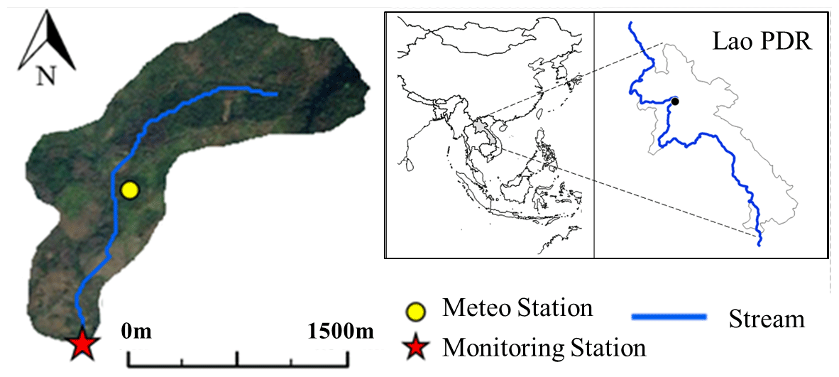
Figure 1 Location of the study area. The study area is located near Luang Prabang in the northern Lao PDR. The gauging and monitoring station is located at the outlet of the catchment, where water level is recorded and where water samples are collected for E. coli concentration measurement. Climate data were measured at the meteorological station.

2.2 Flow and E. coli concentration simulation

HSPF and LSTM models were used to simulate in-stream surface flow, subsurface flow, and E. coli concentration. HSPF and LSTM are popular models (Bicknell et al., 1997; Ahmadisharaf and Benham, 2020; Kratzert et al., 2019). Both models have been used for hydrological and water quality simulations (Peterson et al., 2020; Isikdogan et al., 2017; Ahmed et al., 2014). In the HSPF, the simulation of surface and subsurface flow and of E. coli concentration was carried out in three steps: (1) building the model, (2) conducting sensitivity analysis based on Latin hypercube–one factor at a time (LH-OAT), and (3) calibrating the model using the Newton algorithm (Nash, 1984). The schematic of the LSTM simulation is shown in Fig. 2. The first step in building this model was data preparation (Fig. 2a). LSTM then simulated surface and subsurface flow with weather data (Fig. 2b). Finally, we estimated the E. coli concentration at 6 min intervals using rainfall, bacteria source, land-use change, and surface and subsurface flow (Fig. 2c). The fecal matter from the E. coli sources was assumed to be evenly distributed in the catchment. The monthly E. coli source data are presented in Fig. S1b. The time-series data of the E. coli source were used as input for the E. coli simulation.

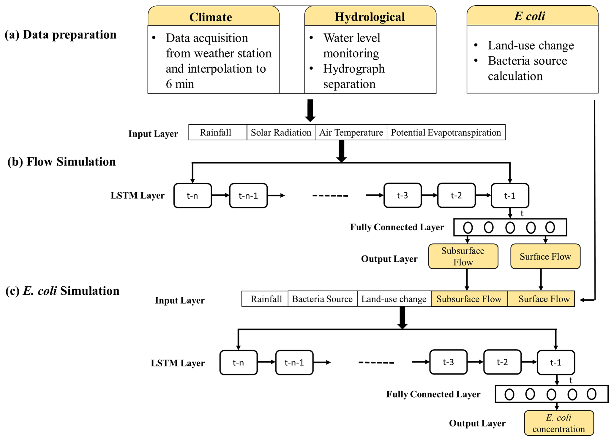
Figure 2 Structure of the LSTM model. Environmental data are used to predict surface flow and subsurface flow. Simulated flows along with bacteria source, land-use information, and rainfall are used to simulate E. coli concentration. The “n” represents the length of input data used by LSTM.

2.2.1 HSPF

The HPSF model is a process-driven model that simulates processes at the catchment scale (Bicknell et al., 1997). It has been extensively used to model the fate and transport of E. coli in catchments (Ahmadisharaf and Benham, 2020; Chin et al., 2009) and to develop total maximum daily loads of E. coli at various locations (Mishra et al., 2018; Yagow et al., 1998). The original software was written in the FORTRAN programming language. The Hydrological Simulation Program Python (HSP2) was recently developed based on the Python programming language (van Rossum, 2007). HSP2 is a platform-independent software that extends the functionality of HSPF by allowing the use of dynamic variables and easier management of input and output files (Heaphy et al., 2015). The HSPF simulates the hydrological regimes by discretizing the catchment into pervious and impervious hydrological response units (HRUs). Evapotranspiration, surface retention, surface infiltration, interflow, baseflow, and deep percolation are simulated at pervious HRUs, whereas surface retention and surface flow are simulated at impervious HRUs (Bicknell et al., 1997). The simulation of in-stream E. coli concentration in HSPF is based on a first-order kinetics approach, considering the decay rate (Fonseca et al., 2014). Detailed descriptions of hydrological and E. coli simulations can be found in Bicknell et al. (1997). For this study, we converted the original FORTRAN code of the E. coli module of HSPF into the Python programming language. This allowed us to incorporate more efficient use of input data, such as the annual change in land use and the monthly bacterial source.

In our study, HRUs were divided into four groups based on land use: “Forest”, “Fallow”, “Teak”, and “Annual” crops. Among land uses, we did not consider any imperviousness in Forest and Fallow. We considered 2 % and 1 % imperviousness for the Teak and Annual crop land uses (Patin et al., 2018). We selected 13 and 4 parameters for each land use for the sensitivity analysis of hydrological and E. coli simulations, respectively (Tables 1 and S1). The total number of parameters for hydrological and E. coli simulation were 52 and 18, respectively. In model calibration, we selected the 25 most sensitive parameters of the hydrological simulation and all parameters of the E. coli simulation. Sensitivity analysis and model calibration were conducted based on the LH-OAT and the Newton algorithm, respectively. A detailed explanation of the LH-OAT and the Newton algorithm can be found in the Supplement (Sect. S4).

Table 1 Optimal values and range of HSPF parameters for surface and subsurface flows and E. coli concentration. Bold parameters were optimized during the flow calibration process. All parameters related to E. coli were optimized during model calibration.

2.2.2 LSTM

In the data preparation step (Fig. 2a), our data were converted to the 6 min frequency. This was carried out by interpolating the hourly weather data. Rainfall data were already available at 6 min for 2011 and 2012, while for 2013 to 2018 they were available at 1 min frequency and were aggregated into a 6 min time series. For E. coli concentration, the values nearest to a 6 min step were used as representative of that time step. We then built the LSTM model to simulate surface and subsurface flow using the validated model structure (Abbas et al., 2020) (Fig. 2b). It uses historical data of rainfall, solar radiation, air temperature, and potential evapotranspiration to simulate surface and subsurface flow. To simulate the output at a time step “t”, LSTM uses the data of previous “n” time steps as inputs (Chollet, 2017). The inputs from previous “n” time steps are used by LSTM to predict the output at the next time step “(t+1)”. These time steps are called “lookback” steps (Chollet, 2017). The simulated surface and subsurface flows from the LSTM were applied to simulate the E. coli concentration (Fig. 2c). We adopted a bacterial source and land-use information as an input for the LSTM. The preprocessing of the data before feeding the neural network can have a significant impact on the performance (Banhatti and Deka, 2016). Therefore, we compared the performance of the model by transforming the E. coli concentration using the min–max transformation and the logarithmic transformation. The min–max transformation results in data between 0 and 1, while logarithmic transformation transforms the data on a logarithmic scale. To investigate the impact of land-use change on in-stream E. coli concentrations, we conducted E. coli simulations in two scenarios. In scenario 1, we used the land-use change and E. coli source information separately. In scenario 2, the number of input features was reduced by multiplying the E. coli source by land-use change. In this way, we calculated the E. coli source per area for each land use and used this as input instead of using land use and E. coli information as separate input features.

LSTM is a special recurrent neural network designed to extract temporal features from sequence data (Hochreiter and Schmidhuber, 1997). An LSTM cell is the basic building block of the LSTM (Fig. S2). It consists of three “gates” and two “states”. The gates are “forget”, “update”, and “output”, which decide what information to forget, allow in, and allow out from the LSTM “memory”, respectively. The states act as a memory or information carrier across time. The equations describing the functions of gates and states are as follows:

$$\begin{array}{}\text{(1)}& {\displaystyle }{C}_{\mathrm{c}}^{<t>}=\tanh \left(W_{\mathrm{c}}[h^{<t-\mathrm{1}>},x^{<t>}]+b_{\mathrm{c}}\right),\text{(2)}& {\displaystyle }{\mathrm{\Gamma }}_f=\mathit{\sigma }\left(W_f\right[c^{<t-\mathrm{1}>}{x}^{<t>}]+b_f),\text{(3)}& {\displaystyle }{\mathrm{\Gamma }}_o=\mathit{\sigma }\left(W_o\right[c^{<t-\mathrm{1}>}{x}^{<t>}]+b_o),\text{(4)}& {\displaystyle }{\mathrm{\Gamma }}_u=\mathit{\sigma }\left(W_u\right[c^{<t-\mathrm{1}>}{x}^{<t>}]+b_u),\text{(5)}& {\displaystyle }{C}^{<t>}={\mathrm{\Gamma }}_u*C_{\mathrm{c}}^{<t>}+{\mathrm{\Gamma }}_f*C^{<t-\mathrm{1}>},\text{(6)}& {\displaystyle }{h}^{<t>}={\mathrm{\Gamma }}_o*\tanh C^{<t>}.\end{array}$$

The symbol * in the above equations represents element-wise multiplication. The behavior of each gate is controlled by the weights (W) and biases (b) associated with them. Gate output is further modified by a nonlinear function (σ). At each time step (t), the prospective cell state $\left(C_{\mathrm{c}}^{<\mathrm{t}>}\right)$ is calculated based on the output from the previous time step $\left(h^{<t-\mathrm{1}>}\right)$ and the input from the current time step $\left(x^{<t>}\right)$ (Eq. 1). The notation $W_{\mathrm{c}}\left[h^{<t-\mathrm{1}>}{x}^{<t>}\right]$ represents point-wise multiplication of new inputs and previous hidden state with the weight matrix W_c and then adds their output. This prospective cell state ($C_{\mathrm{c}}^{<t>}$), along with the output from the “forget” and “update” gates, decides the current cell state $\left(c^{<t>}\right)$ (Eq. 5). The current cell state and output gate control the output values from LSTM ($h^{<t>})$ forming the so-called hidden state (Eq. 6). The hyperbolic tangent (tanh) is another nonlinearity used in LSTM for the calculation of the cell state (Eq. 1) and the output state (Eq. 6). Equations (1)–(6) are used to calculate the LSTM output, which is then compared with observed values to calculate the error. This study used the mean square error (MSE) as the error metric.

We used the TensorFlow software v1.15 for building the LSTM model (Abadi et al., 2016). We used an Intel^® Core™ i7-9700 processor with a graphics card of NVIDIA GeForce RTX 2080 with 12 GB of dedicated GPU memory, along with 64 GB of random-access memory for simulating surface, subsurface, and E. coli.

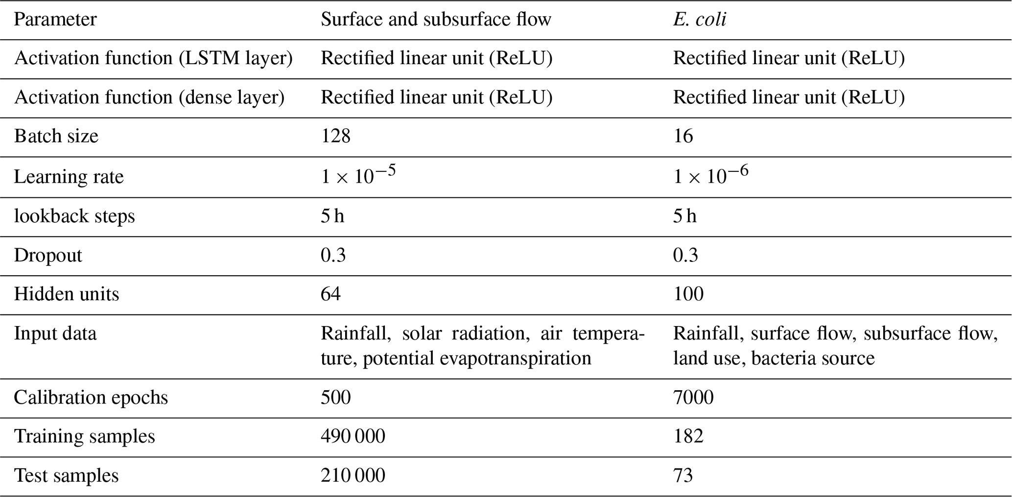
2.2.3 Hyperparameters of LSTM

The structure and performance of the LSTM were controlled by hyperparameters, including the dropout rate, the number of LSTM units, learning rate, lookback steps, and activation functions for both LSTM and the fully connected layer (Table 2). Dropout is a regularization technique that switches off a certain number of nodes in the LSTM (Goodfellow et al., 2016). This simple technique helps break the brittle coadaptation of weights, which hinders generalization to unseen data. This way, dropout prevents overfitting (Srivastava et al., 2014). In the case of overfitting, the model performs better on calibration data, but its performance deteriorates on new unseen data. The number of LSTM units directly corresponds to the learning capacity of LSTM, but it also accounts for more memory and computation. This number determines the size of the weight matrix of an LSTM. The learning rate defines the change in the weights of the neural network during calibration (Goodfellow et al., 2016). A higher number of lookback steps allows LSTM to capture long-term patterns at the cost of an increase in memory consumption and computation. The activation function determines the nonlinearity in the model.

Table 2 Hyperparameters of LSTM for surface flow, subsurface flow, and E. coli concentration simulation.

2.3 Performance statistics

Evaluations to assess the performance of the HSPF and LSTM were conducted using MSE, Nash–Sutcliffe efficiency (NSE), and percent bias (PBIAS) (Nash and Sutcliffe, 1970; Gupta et al., 1999). NSE is useful for interpreting the model performance by generating a dimensionless value as the performance index (Lin et al., 2017). The PBIAS measures the average tendency of the simulated data to be overestimated or underestimated than observed values (Moriasi et al., 2015). The MSE, NSE, and PBIAS were calculated using the following equations:

$$\begin{array}{}\text{(7)}& {\displaystyle }\mathrm{MSE}={\displaystyle \frac{\left[{\sum }_{i=\mathrm{1}}^m{\left(o_i-p_i\right)}^{\mathrm{2}}\right]}{m}},\text{(8)}& {\displaystyle }\mathrm{NSE}=\mathrm{1}-{\displaystyle \frac{\sum (o_i-p_i{)}^{\mathrm{2}}}{\sum (o_i-\stackrel{\mathrm{‾}}{o}{)}^{\mathrm{2}}}},\text{(9)}& {\displaystyle }\mathrm{PBIAS}=\mathrm{1}-{\displaystyle \frac{{\sum }_{i=\mathrm{1}}^m(o_i-p_i)}{{\sum }_{i=\mathrm{1}}^m{o}_i}},\end{array}$$

where p_i is the simulated data, o_i is the observed data, and m is the number of points in the data.

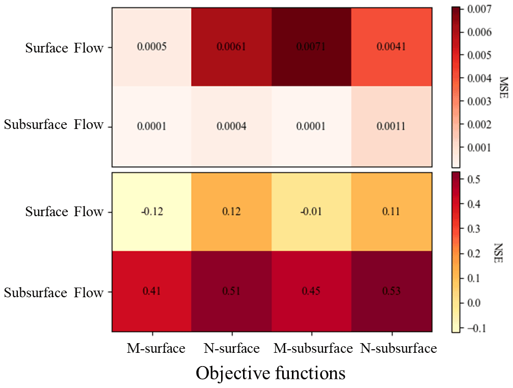
Figure 3 Performance of the HSPF model with different objective functions (e.g., M-surface, N-surface, M-subsurface, and N-subsurface). The color indicates the value of MSE and NSE. M-surface is the objective function based on MSE and surface flow, N-surface is the objective function based on NSE and surface flow, M-subsurface is the objective function based on MSE and subsurface flow, and N-subsurface is the objective function based on NSE and subsurface flow.

3 Results and discussion

3.1 Land-use change and E. coli source

The land-use change from 2011 to 2018 is shown in Fig. S1a. The area of Fallow land use increased from 2011 to 2016, whereas Annual crop area decreased. Teak tree plantations were expanded until 2013 and were retained. Forest land use accounted for about 10 % of the study area from 2011 to 2018. In general, the land-use change was dynamic from 2011 to 2013, whereas its variation diminished from 2016 to 2018. Previous studies have demonstrated that the expansion of Teak trees might increase the surface flow (Ribolzi et al., 2017; Song et al., 2020). Higher runoff at the soil surface may cause a higher inflow of E. coli with surface flow. The monthly E. coli source in the catchment decreased from 2×10¹⁵ in 2011 to 3×10¹⁴ in 2018 (Fig. S1b). This decrease in the E. coli source is caused by the decrease in manpower needed in Teak tree plantations and in Fallow plots compared to the Annual crop (Fig. S1a) (Boithias et al., 2021b).

3.2 Sensitivity analysis and optimization result

The sensitivity results for the flow simulation are shown in Fig. S3, and the most sensitive parameters are listed in Table S2. The interflow and infiltration-related parameters were the most sensitive parameters for surface and subsurface flows. Manning's “n” value (NSUR) for Teak and Fallow land uses was among the 10 most sensitive parameters. Kim et al. (2017) suggested that Manning's coefficient value is the most sensitive parameter in the hydrological simulation of tropical headwater catchments, such as the Houay Pano catchment in the northern Lao PDR. The groundwater recession rate (AGWRC) and soil infiltration capacity (INFILD) were sensitive to subsurface flow. In Annual crop land use, infiltration capacity (INFILT) and upper zone storage (UZSN) were the most sensitive parameters. Abbas et al. (2020) demonstrated that INFILT is the most sensitive parameter for subsurface flow in tropical subcatchments.

The sensitivity analysis results for E. coli are shown in Fig. S4 and Table S3. The parameters related to the transport of E. coli on the land surface (e.g., WSQOP, SQOLIM_MF) were more sensitive than other parameters. IOQC and AOQC were the least sensitive parameters. These parameters are related to E. coli transport in interflow and baseflow (Bicknell et al., 1997). This implies that the in-stream E. coli concentration at the study site is mainly driven by surface flow (Boithias et al., 2021b). A previous study also demonstrated that 89 % of in-stream E. coli concentrations were driven by surface flow (Boithias et al., 2021b). Figure 3 shows the model performance dependent on different objective functions. We found that the model performance was better when the NSE was selected as the objective function. The NSE of the surface and subsurface flow was positive by optimizing with NSE. However, the NSE value for surface flow was negative when the objective function was MSE during the optimization. Negative NSE indicated an “unsatisfactory” performance range (Moriasi et al., 2015).

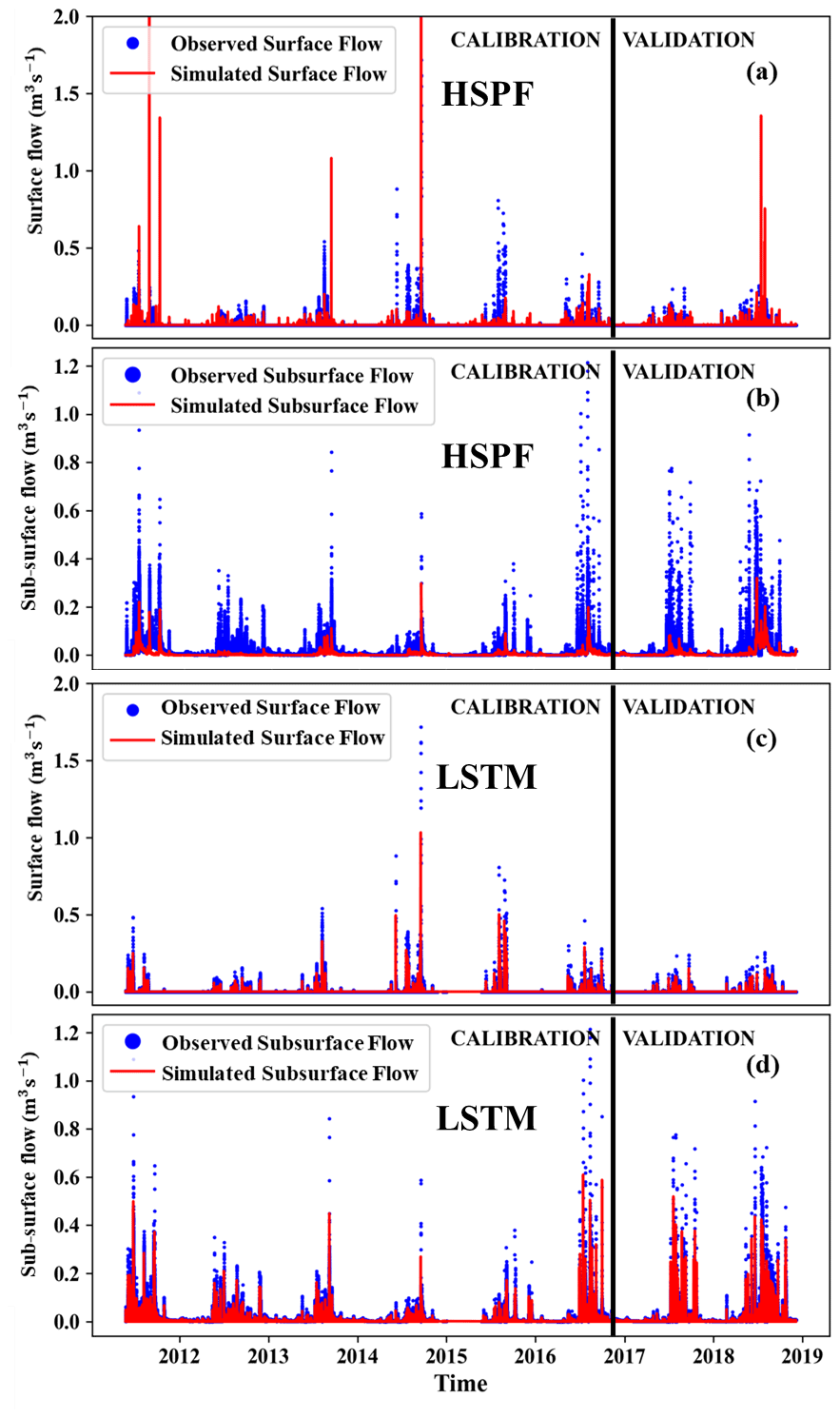
Figure 4 Hydrological simulation from HSPF and LSTM: (a) simulated and observed surface flow from HSPF, (b) simulated and observed subsurface flow from HSPF, (c) simulated and observed surface flow from LSTM, and (d) simulated and observed subsurface flow from LSTM.

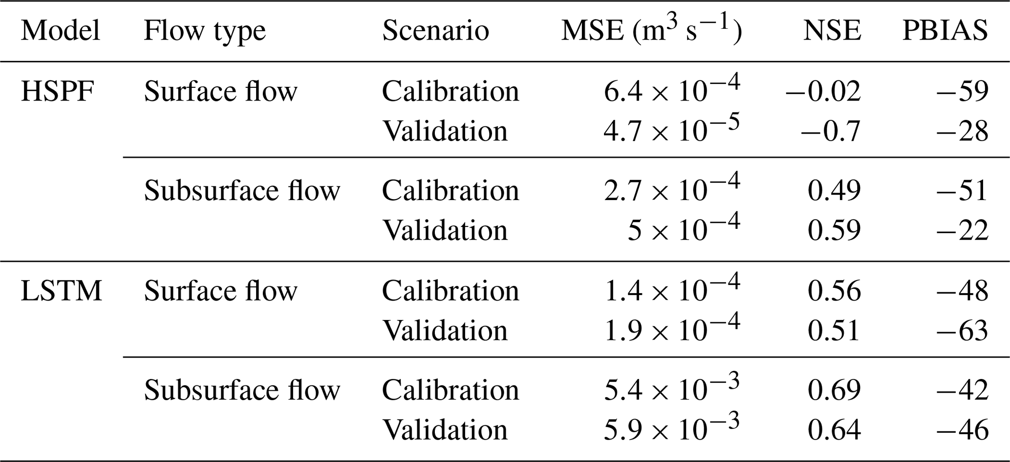
Table 3 Performance metrics of HSPF and the LSTM model for surface and subsurface flow.

3.3 Flow simulation

The simulated surface and subsurface flows using the HSPF are plotted in Fig. 4. We found that the simulated subsurface flow was underestimated compared to the observations. Although surface flow from the HSPF followed the trend and peaks of observations, this model yielded a negative NSE value, indicating that the model simulation was unacceptable (Moriasi et al., 2015) (Table 3). The NSE values for subsurface flow from HSPF were 0.49 and 0.59 for calibration and validation, respectively. Hence, the HSPF model was better at simulating subsurface flow than surface flow. In particular, the simulated surface flow was underestimated compared to the observations. The average values of INFILT and UZSN were 0.36 and 1.22, respectively, which were larger than those reported in previous studies (Lee et al., 2020). INIFILT controls the overall division of available moisture into the surface and subsurface (Bicknell et al., 1997). The parameter UZSN influences the evapotranspiration process (Bicknell et al., 1997). This underestimation of surface flow using HSPF is consistent with a previous study (Kim et al., 2017). We also investigated the impact of underestimation and overestimation of the flow by plotting flow duration curves (Fig. S5). Although both flows can capture the peak flow, the simulated subsurface flow was still underestimated compared to the observed subsurface flow.

The simulated surface and subsurface flows using the LSTM model are plotted in Fig. 4. The NSE values for the calibration period were 0.56 and 0.69 for surface and subsurface flow, respectively. The corresponding validation NSE values of the surface and subsurface flows were 0.51 and 0.64, respectively. These results indicate that the LSTM had a satisfactory performance for both the calibration and validation periods according to the criteria of Moriasi et al. (2015). LSTM overcame the problem of the HSPF model underestimating subsurface flow. In addition, the peak surface flows from the LSTM were similar to observations. The observed and simulated flows in storm events are presented in Figs. S6–S11. The simulated surface flow by HSPF followed the rainfall events more closely as compared to that of LSTM. The peaks in surface flow in Fig. S8 are completely missed by LSTM but captured by the HSPF model. We also noted that LSTM can follow the observed trends in surface and subsurface flow more closely than the HSPF (Figs. S6, S9, S10). The falling limb from the predicted subsurface flow of LSTM is gentle and follows the observed pattern (Figs. S9–S11). This leads to increased NSE values for both surface flow as well as for subsurface flow. The hyperparameters of the LSTM are described in Table 2. The rectified linear unit (ReLU) was chosen as the activation function for the LSTM output. Because the simulated E. coli should be positive, we chose ReLU, which cannot produce negative values from the model (Nair and Hinton, 2010). The optimal batch size and LSTM units were 128 and 64, respectively. The optimal value of the lookback steps was 50, which is equal to 5 h of input data.

We analyzed the model performance for surface and subsurface flows during storm events (Fig. 5). The events were selected in which the peak flow exceeded 0.2 m³ s⁻¹. The performance of LSTM is considerably better than that of HSPF for most storm events. In surface flow, the average MSE of LSTM and HSPF was $\mathrm{1.1}\times {\mathrm{10}}^{-\mathrm{4}}$ and $\mathrm{6.1}\times {\mathrm{10}}^{-\mathrm{4}}$ (m³ s⁻¹), respectively. The NSE values from LSTM varied from 0.2 to 0.6, whereas those of HSPF ranged from −1.0 to 0.4. We found that the NSE values from the HSPF vary considerably depending on storm events. On 11 June 2015, the NSE value of HSPF was as high as 0.4, whereas for some other dates it was below 0. Although the subsurface flow of the HSPF provided better model performance than surface flow simulation, this model still presented an unacceptable result, with a negative NSE value.

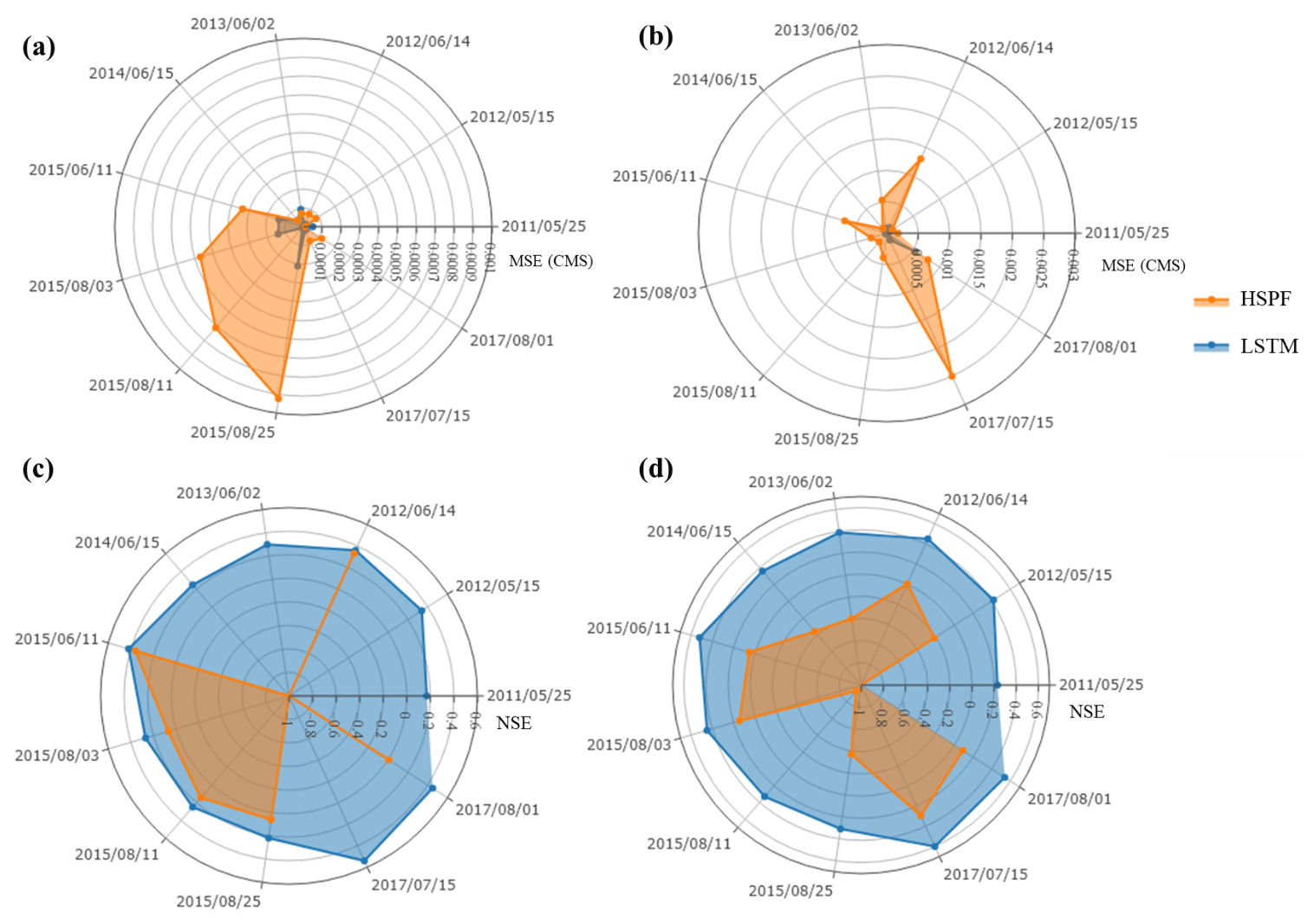
Figure 5 Comparison of the hydrological simulation during storm events: (a) MSE value of the surface flow, (b) MSE value of the subsurface flow, (c) NSE value of the surface flow, and (d) NSE value of the subsurface flow.

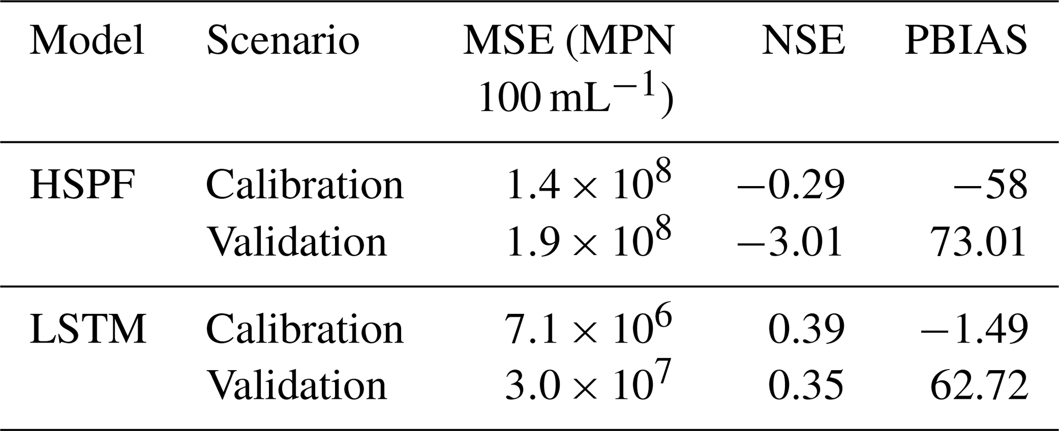
Table 4 Performance metrics of HSPF and LSTM for E. coli concentration simulation.

3.4 E. coli simulation

Figure 6 shows the temporal distribution of E. coli concentration using HSPF and LSTM. The E. coli concentration from HSPF was overestimated. The performance matrices of the HSPF were also worse than those of the LSTM (Table 4). In particular, the HSPF simulation presented a PBIAS value of 73, indicating an overestimation of E. coli concentration (Moriasi et al., 2015). Ackerman and Weisman (2014) reported that the E. coli from HPSF was overestimated compared to observation. The overestimation of simulated E. coli at tropical sites has also been observed by Kim et al. (2017). E. coli simulation from LSTM is satisfactory in both calibration and validation periods according to the criteria set by Moriasi et al. (2015). In contrast, the HSPF result can be regarded as “unsatisfactory” in both the calibration and validation periods. These results implied that LSTM could generate acceptable performances and had good agreement between the observed and simulated E. coli.

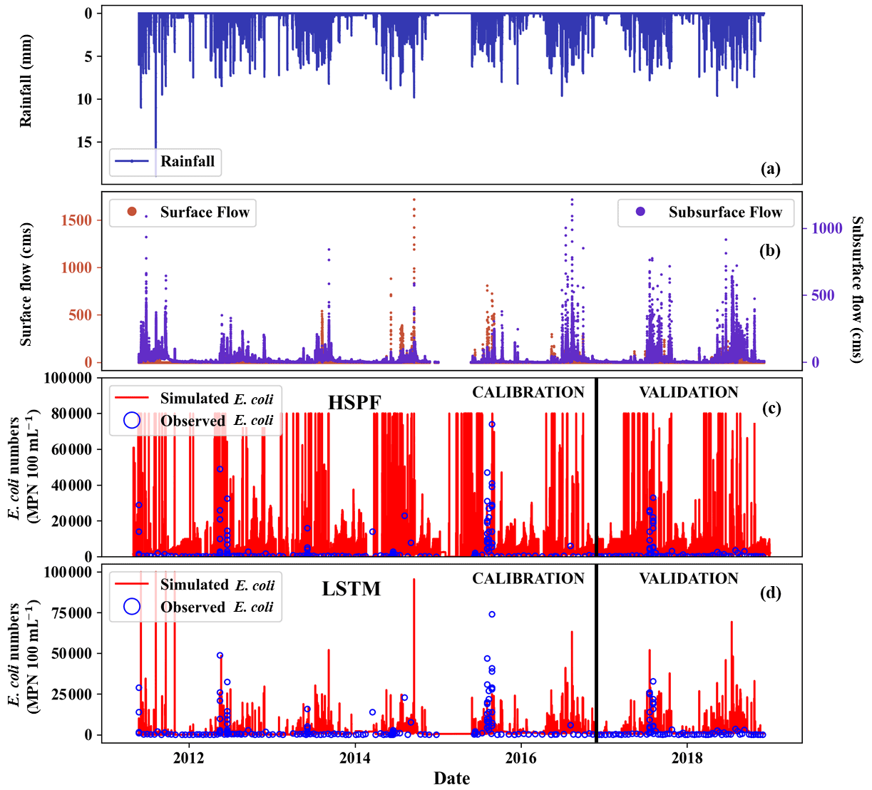
Figure 6 E. coli simulation from LSTM and HSPF: (a) measured rainfall, (b) observed surface and subsurface flow, (c) simulated and observed E. coli concentration using HSPF, and (d) simulated and observed E. coli concentration using LSTM.

The simulation results during the storm events using both the HSPF and LSTM models are shown in Figs. 7 and S6–S11. Figure 8 shows two storm events from the validation data during July and August 2017, whereas the other figures show the storm events from the calibration data. In general, the simulated E. coli by HPSF and LSTM were overestimated and underestimated, respectively. This difference might be caused by the fact that E. coli from HSPF is more responsive to surface flow, whereas E. coli from LSTM is more influenced by subsurface flow (Ackerman and Weisman, 2014). The sensitivity analysis of HSPF also demonstrated that the influence of interflow and baseflow on E. coli is weaker than that of surface flow because the parameters IOQC and AOQC are the least sensitive parameters for E. coli simulation. Both parameters affect the E. coli concentration in interflow and baseflow (Bicknell et al., 1997). The simulated E. coli of LSTM rose sharply and dropped slowly, similarly to the observations, whereas that of the HSPF decreased steeply (Figs. S6–S11). Although both models simulated the peak time of the E. coli correctly, the HSPF was limited in its ability to simulate the slope of the falling limb. This performance difference between models was caused by the extent of the influence from hydrological variables (e.g., rainfall, surface flow, and subsurface flow) on model output. LSTM was effective in reflecting the response of the output to hydrologic variables (Kratzert et al., 2019).

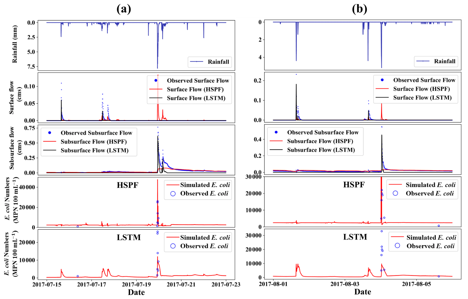
Figure 7 E. coli concentration simulated by HSPF and LSTM during 15–22 July (a) and 1–5 August 2017 (b). Both storm events were affiliated in the validation period.

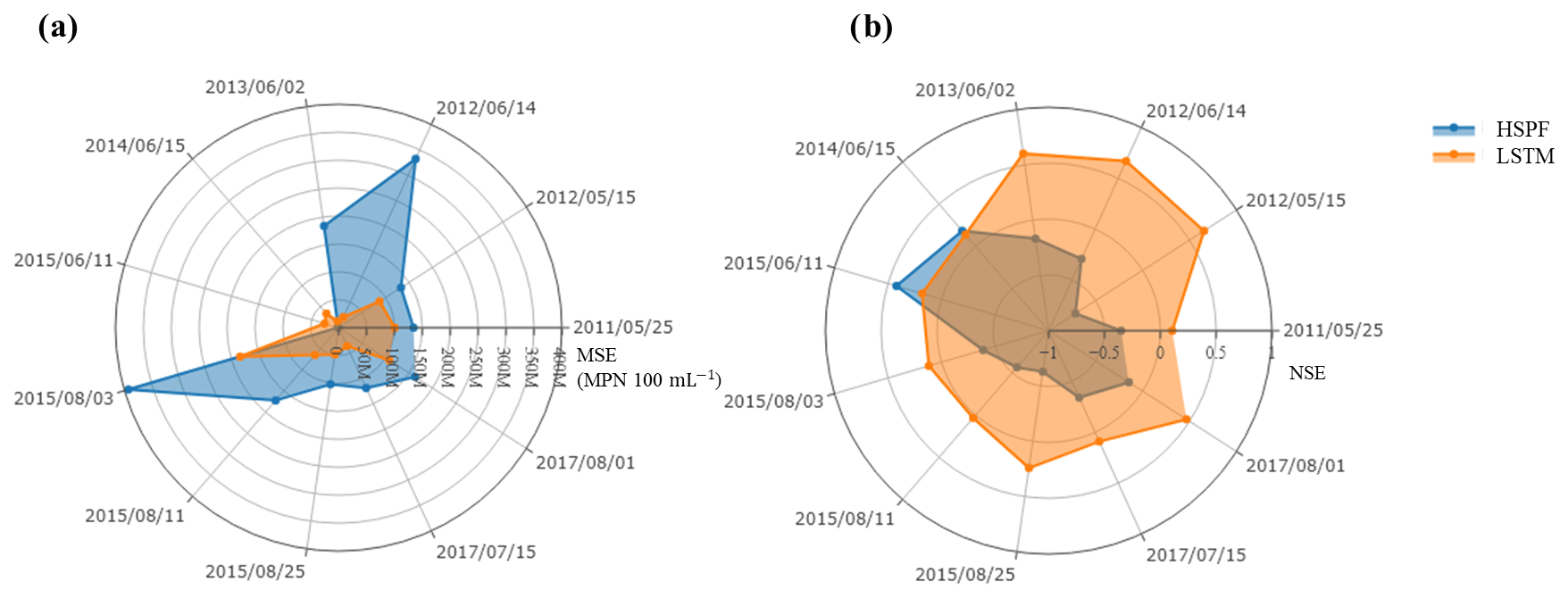
Figure 8 Comparison of the E. coli simulation during storm events: (a) MSE values and (b) NSE values.

We observed that both HSPF and LSTM simulated peaks even when the observed data did show corresponding peaks (Figs. S8 and S11). The peaks predicted in Fig. S8 are solely from HSPF, while the peak event in Fig. S11 is predicted by both HSPF and LSTM models. This shows the efficacy of both calibrated models. We could conclude from Fig. S11 that the lack of an observed peak is more likely because of missing observation. However, a similar conclusion cannot be drawn for all the predicted E. coli peaks in Fig. S8 because of contradicting results of LSTM and HSPF.

The performance metrics for the LSTM and HSPF models during storm events are shown in Fig. 8. In general, we observed better LSTM performance than HSPF in terms of NSE and MSE values. The HSPF model performed better than the LSTM for only two storm events: on 15 June 2014 and 11 June 2015. For the remaining storm events, the NSE values from LSTM are higher than those of the HSPF – an NSE range from 0.20 to 0.65. Similarly, for MSE values, the LSTM was superior to the HSPF for all storm events except for the storm events on 15 June 2014 and 11 June 2015.

We observed the impact of logarithmic and min–max transformations on the model performance (Fig. 9). The results of the logarithmic transformation were closer to the observations than the min–max transformation by showing an NSE of 0.57. A negative PBIAS value was obtained in logarithmic transformation. This indicated that the simulated E. coli from logarithmic transformation was underestimated, whereas the result of the min–max transformation was overestimated. This behavior can be attributed to the ability of min–max scaling to be more sensitive to outliers (Chuang et al., 2010). As a result, if a better accuracy during storm events is required, the target variable can be transformed on a logarithmic scale prior to calibration. This is because log transformation can reduce the effect of outliers (Singh and Kingsbury, 2017). It has been reported that log transformation can improve the performance of data-driven models when the data contain outliers (Zheng and Casari, 2018).

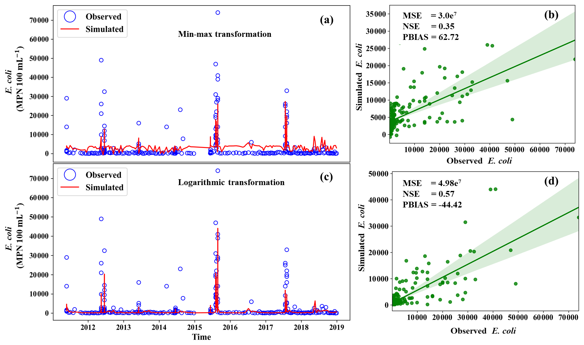
Figure 9 Comparison of E. coli concentration simulation with the transformation method: panels (a) and (c) indicate the E. coli simulation using min–max transformation and logarithmic transformation, respectively. Panels (b) and (d) indicate the scatter plot of E. coli using min–max transformation and logarithmic transformation, respectively.

3.5 E. coli response to land-use change

We investigated the impact of land-use change and bacterial sources on the in-stream E. coli concentration simulation (Fig. 10). In scenario 1, we used land-use change time-series information (Fig. S1a) and bacterial source information (Fig. S1b). In scenario 2, we divided the bacterial source by the fraction of each land use (Fig. S2c). In scenario 1, we observed a larger variation in E. coli concentration from 2014 to 2018 (Fig. 10a), whereas in scenario 2, the variation in E. coli was smaller than that in scenario 1 (Fig. 10b). This variation in E. coli was due to land-use change in scenario 1. In particular, E. coli in 2016 was less than in other years because the Annual crop land use decreased. On the other hand, the variation in E. coli was not observed in scenario 2 from 2015 to 2017. Neither scenario showed a significant response from 2011 to 2014. During these years, the rise in Fallow land use was complemented by a decrease in Annual crop land use.

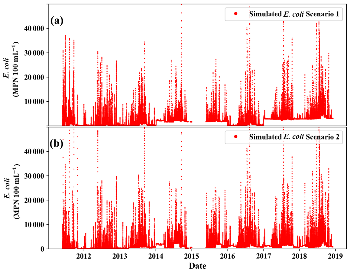
Figure 10 Simulated E. coli concentration with changes in E. coli sources with land-use change scenarios. Scenario 1 used land-use change and bacterial source information. Scenario 2 used the bacterial source by the fraction of each land use.

3.6 Limitations and future research

Transport of soil particles by surface flow and suspended sediments within the stream plays a crucial role in the fate and transport of E. coli (Thupaki et al., 2013). Several studies have emphasized the importance of particle size (Cho et al., 2010), adsorption to soil and sediment particles (Palmateer et al., 1993), and resuspension of E. coli (Kim et al., 2017) with streambed sediments for modeling the fate and transport of E. coli at the catchment scale. In this study, we considered neither sediment transport nor the attachment/detachment of E. coli on/from soil particles and suspended sediments. Several studies have been conducted on the monitoring and modeling of E. coli without considering sediment transport (Ahmadisharaf and Benham, 2020; Mishra et al., 2018). However, the need for its inclusion has been indicated elsewhere (Pandey and Soupir, 2013). To model sediment transport, additional data on suspended sediment concentration are required to build both the HSPF and deep-learning-based models. Therefore, this modeling can be further improved by collecting sediment-related data and modeling sediment transport along with E. coli concentration.

The deep-learning-based approach can yield high model performance, but it has the limitation in terms of explainability and interpretability (Molnar, 2020). The neural networks are generally considered black boxes, and the question of interpreting them is still an open research problem (Mitchell, 2021; Tiddi, 2020). Several methods have been proposed to interpret the behavior of neural networks (Molnar et al., 2020). Explaining the output of neural networks can enhance the confidence of decision makers (Lipton, 2018). Therefore, we propose future research involving deep-learning models will benefit if the questions of interpretability and explainability are considered along with a model's prediction performance.

Deep-learning models are based upon the independent and identically distributed (IID) assumption, which means that the validation data are expected to have the same distribution as that of the training data (Kawaguchi et al., 2017). However, this is not a realistic assumption, and it is considered one of the challenges for researchers in machine learning (Bengio et al., 2021). Thus, in order to build regional or global hydrological models, the deep-learning model should be trained on catchment data from diverse catchments. Several researchers have adopted this approach to build regional models for streamflow prediction (Anderson and Radic, 2021; Kratzert et al., 2019; Xiang et al., 2021). However, a similar approach for building regional water quality models will be more challenging due to the scarcity of water quality data. We hope that the lessons from this study can be used as a guideline to train neural networks on regional water quality data.

4 Conclusions

In this study, we simulated the transport of bacteria in a headwater catchment of the northern Lao PDR at 6 min time steps. The main findings of this study are summarized as follows.

• Both the LSTM and HSPF models can accommodate land-use change and bacteria-source variation with time.

• The performance of the surface and subsurface flow simulation of LSTM was superior for both the calibration and validation steps when compared with the HSPF. The LSTM provided accurate surface and subsurface flow results by showing NSE values of 0.51 and 0.59, respectively, whereas the HSPF showed −0.7 and 0.55 of NSE.

• Our LSTM model showed better performance compared to HSPF for E. coli simulation. The NSE values of the HSPF and LSTM were −3.01 and 0.35, respectively. We found that the LSTM model can respond to changes in land use.

This study shows that deep-learning-based models are an efficient alternative to process-based models to simulate E. coli in a given catchment. Because LSTM can generate reasonable E. coli simulations, it could be applied to provide effective strategies for thwarting diseases that wreak havoc on human health. Therefore, a deep-learning approach can be useful in developing better water sustainability and management.