the Creative Commons Attribution 4.0 License.
the Creative Commons Attribution 4.0 License.
 | 22 Sep 2021
A scaling procedure for straightforward computation of sorptivity
Laurent Lassabatere
Pierre-Emmanuel Peyneau
Deniz Yilmaz
Joseph Pollacco
Jesús Fernández-Gálvez
Borja Latorre
David Moret-Fernández
Simone Di Prima
Mehdi Rahmati
Ryan D. Stewart
Majdi Abou Najm
Claude Hammecker
Rafael Angulo-Jaramillo
Sorptivity is a parameter of primary importance in the study of unsaturated flow in soils. This hydraulic parameter is required to model water infiltration into vertical soil profiles. Sorptivity can be directly estimated from the soil hydraulic functions (water retention and hydraulic conductivity curves), using the integral formulation of Parlange (1975). However, calculating sorptivity in this manner requires the prior determination of the soil hydraulic diffusivity and its numerical integration between initial and final saturation degrees, which may be difficult in some situations (e.g., coarse soil with diffusivity functions that are quasi-infinite close to saturation). In this paper, we present a procedure to compute sorptivity using a scaling parameter, cp, that corresponds to the sorptivity of a unit soil (i.e., unit values for all parameters and zero residual water content) that is utterly dry at the initial state and saturated at the final state. The cp parameter was computed numerically and analytically for five hydraulic models: delta (i.e., Green and Ampt), Brooks and Corey, van Genuchten–Mualem, van Genuchten–Burdine, and Kosugi. Based on the results, we proposed brand new analytical expressions for some of the models and validated previous formulations for the other models. We also tabulated the output values so that they can easily be used to determine the actual sorptivity value for any case. At the same time, our numerical results showed that the relation between cp and the hydraulic shape parameters strongly depends on the chosen model. These results highlight the need for careful selection of the proper model for the description of the water retention and hydraulic conductivity functions when estimating sorptivity.
- Article
(1457 KB) - Full-text XML
- Companion paper
- BibTeX
- EndNote


Soil sorptivity represents the capacity of a soil to absorb or desorb liquid by capillarity and is therefore one of the key factors for modeling water infiltration into soil (Cook and Minasny, 2011). Knowledge of soil sorptivity is also important when deciphering soil physical properties, such as hydraulic conductivity, from infiltration tests (e.g., Lassabatere et al., 2006). Sorptivity is incorporated in a wide range of infiltration models (Angulo-Jaramillo et al., 2016; Lassabatere et al., 2009, 2014, 2019). Sorptivity varies depending on initial and boundary conditions (e.g., water contents). However, calculated sorptivity values can also vary depending on the chosen soil hydraulic model, making it important to assess the impact of such a choice on the computation of sorptivity. In this study, we address this issue and propose a new scaling procedure to simplify its computation.
One of the first equations proposed for the computation of sorptivity was developed by Philip (1957), who modeled the 1D gravity-free water infiltration as
In the above equations, S(θ0,θ1) stands for the sorptivity between θ0 and θ1, stands for the Boltzmann transformation variable, θ0 is the initial water content, θ1 is the final water content corresponding also to the water content applied at the soil surface, and t is the elapsed time. In practical applications, the user must perform numerical modeling of horizontal infiltration using a given set of hydraulic functions and initial and final conditions. Then, the Boltzmann transformation must be computed by integrating the modeled water content profile. This procedure is often time-consuming and subject to numerical instabilities that lead to substantial errors.
To avoid such complexity, Parlange (1975) proposed a formulation that directly relates sorptivity to the hydraulic functions and the initial and final water contents:
where is the hydraulic diffusivity function. Note that several integral expansions were proposed for the computation of sorptivity (Angulo-Jaramillo et al., 2016). This point is beyond the framework of this study and will be the subject of another study. While the above equation provides the diffusivity form for sorptivity determination, it can be equally defined as a function of the hydraulic conductivity function, K(h)=K(θ(h)):
where h is the water pressure head, h0 and h1 are respectively the initial and final water pressure heads, and θ0=θ(h0) and θ1=θ(h1). For the sake of clarity, the functions and are respectively referred to as the “diffusivity” and “conductivity” forms of sorptivity. and are equivalent so long as the water retention function θ(h) is bijective over the water pressure head interval [h0,h1], which is the case when the water pressure head at the surface is lower than the air-entry water pressure head, i.e., h1≤ha. Then, Eq. (3) can be easily deduced from Eq. (2) by a simple change of variable from θ to h:
Otherwise, when the surface water pressure head exceeds the soil air-entry pressure, i.e., , sorptivity must be computed using Eq. (3) (Ross et al., 1996). Indeed, the function θ(h) is no longer bijective over the interval [h0,h1]. Consequently, Eqs. (2) and (3) are no longer equivalent. In this case, the integration involved in Eq. (3) must be divided into two parts, one part integrating over the interval [h0,ha] ensuring the bijectivity of the function θ(h) and the other part retaining the integration interval [ha,h1] corresponding to the saturated part of the integration (Ross et al., 1996). Then, the change of variable from θ to h in the first integral leads to the retrieval of :
The computation of sorptivity with Eq. (2) or Eq. (3) requires a set of hydraulic functions to be chosen from the wide range of available models. Here, we considered five of the most widely used hydraulic models. Firstly, we considered the delta model (d, delta) , which involves Dirac delta functions (stepwise functions) for the description of both the water retention (WR) and hydraulic conductivity (HC) functions. Indeed, this model is often considered for analytical resolutions to the Richards equation and the determination of analytical expressions for water infiltration, like the Green and Ampt approach (Triadis and Broadbridge, 2012). Secondly, we considered the Brooks and Corey (1964) model, referred to as the BC model, since it is among the first hydraulic models of soil physics (Hillel, 1998). The BC model involves power functions for both the WR and HC functions, thus allowing for analytical integration of Eq. (2) and leading to analytical expressions for sorptivity (e.g., Varado et al., 2006). Thirdly, the van Genuchten–Burdine (vGB) model was studied since it has been used for the development of the BEST methods (Beerkan Estimation of Soil Transfer functions) for the characterization of soil hydraulic properties (Lassabatere et al., 2006; Yilmaz et al., 2010; Bagarello et al., 2014). The vGB model combines the van Genuchten (1980) model with Burdine's condition for the WR function and the Brooks and Corey (1964) model for the HC function. Fourthly, we considered the van Genuchten–Mualem (vGM) model that combines the van Genuchten (1980) model with Mualem's condition for the WR function and the Mualem (1976) capillary model for the HC function. The vGM is among the most widely used models and often used for the numerical modeling of flow in the vadose zone (Šimůnek et al., 2003). Lastly, the Kosugi (KG) model (Kosugi, 1996), was also considered since it relates the water retention function to physical characteristics of the soil pore size distribution assuming log-normal distributions.
These five models have the following mathematical expressions (Triadis and Broadbridge, 2012; Brooks and Corey, 1964; van Genuchten, 1980; Mualem, 1976; Kosugi, 1996; Nasta et al., 2013):
delta model:
BC model:
vGB model:
vGM model:
KG model:
where H stands for the one-sided Heaviside step function: , (Triadis and Broadbridge, 2012); and “erfc” stands for the complementary error function. These models involve several specific hydraulic shape parameters and the following common scale hydraulic parameters: residual water content, θr, saturated water content, θs, scale parameter for the water pressure head, hg (i.e., hd, hBC, hvGB, hvGM, or hKG), and saturated hydraulic conductivity, Ks. The delta and BC models involve a non-null air-entry water pressure head, hd and hBC, meaning that air needs a nonzero suction to enter into the soil and start to desaturate it. For the sake of simplicity, the scale parameter for the water pressure head is fixed at the air-entry pressure head, i.e., hg=hd and hg=hBC, respectively.
The computation of sorptivity by applying Eq. (2) or (3) to hydraulic models, and in particular to those selected for this study, i.e., Eqs. (6)–(10), is quite tricky, given the complexity of the hydraulic functions. Such computation might exhibit the following shortcomings. First of all, the diffusivity functions must be determined analytically, by multiplying the hydraulic conductivity by the derivative of the water pressure head with regards to water content, which may involve complex algebraic operations. Then, the integration involved in the right-hand side of Eq. (3) may lead to numerical indetermination for very low initial water pressure heads, in the case of very dry initial conditions. Meanwhile, the integration involved in the right-hand side of Eq. (2) may pose numerical shortcomings for infinite hydraulic diffusivity, which is the case for some of the hydraulic functions detailed above, Eqs. (6)–(10).
In this study, we propose a specific scaling procedure to avoid all these shortcomings and to simplify the computation of sorptivity for the hydraulic models described in Eqs. (6)–(10) under the boundary conditions of a slightly positive water pressure head at surface and relatively dry initial conditions. We focus on these conditions since they constitute the most common experimental conditions for most water infiltration experiments and related procedures for characterizing soil hydraulic properties (Angulo-Jaramillo et al., 2016). In particular, these conditions feature the Beerkan method that involves pouring water into a ring placed on the ground (Braud, 2005; Lassabatere et al., 2006).
The rest of the paper is organized as follows. The theory section details the scaling procedure that relates the square sorptivity to the (i) square scaled sorptivity, , which we show is equal to the parameter cp, and (ii) the product of scale parameters and correcting factors accounting for the contribution of initial water contents. The square scaled sorptivity corresponds to the sorptivity of a unit soil (unit value for all the scale parameters, except the residual water content fixed at zero) and for the whole range of water pressure heads, i.e., . It depends only on the soil hydraulic shape parameters, and its determination features the main algebraic complexity of the whole scaling procedure; the rest relies on simple algebraic operations (multiplication and sums). It is then computed for the hydraulic models defined by Eqs. (6)–(10), either analytically when feasible or numerically, otherwise. For each model, it is computed and tabulated as a function of a shape index that characterizes the spreads of the water retention function (from gradual to stepwise shapes, corresponding to soils with a broad or a very narrow pore size distribution, respectively). The evolution of the square scaled sorptivity versus the shape index is compared and discussed between models. In the last section, we illustrate the application of the proposed scaling procedure. We show how the tabulated values of the square scaled sorptivity cp can be used to upscale sorptivity and easily provide the sorptivity corresponding to a zero water pressure head at the surface for relatively small initial water contents.
2.1 Global scaling procedure
The proposed scaling procedure relies on two main steps already used in some previous studies: (i) relating the actual square sorptivity to the maximum square sorptivity by isolating the effect of initial and final conditions (h0 and h1) and (ii) scaling hydraulic functions and sorptivity to split the contributions of shape and scale parameters and facilitate the computation of . In our case, we consider that the final conditions always involve a null water pressure head, h1=0, and saturated conditions, θ1=θs, while initial conditions (h0,θ0) may vary.
2.1.1 Isolating the effect of initial conditions
The first step of the proposed procedure involves the work of Haverkamp et al. (2005), who isolated the contributions of the initial and final conditions to sorptivity. These authors considered that, at dry initial states () and a zero water pressure head at surface (i.e., h1=0 and θ1=θs), the following approximation applied:
where K0 corresponds to the initial hydraulic conductivity K0=K(θ0). The parameter is a proportionality constant that depends only on the hydraulic shape parameters (Haverkamp et al., 2005). By combining both expressions in Eq. (11), the sorptivity, S2(θ0,θs), can be defined as the product of three different terms that account for the respective contributions of the shape parameters (lumped into the proportionality constant cp), the scale parameters, , Ks, and θs, and initial conditions, θ0:
Equation (12) offers an accurate and practical approximation for the computation of sorptivity in the case of Beerkan runs, i.e., for a zero water pressure head imposed at the soil surface, h1=0. Equation (12) was frequently used for the treatment of Beerkan data and in particular in all BEST methods (Lassabatere et al., 2006; Yilmaz et al., 2010; Angulo-Jaramillo et al., 2019). However, it addresses the case of soils with null residual water content, θr=0, and without any air-entry pressure head, ha=0. In addition, it was developed and used for the vGB model.
In this study, we adapt Eq. (12) to any type of hydraulic model, including those with non-null residual water contents, θr>0, and air-entry water pressure heads, ha<0. First of all, we consider that θr must be accounted for, and we replace Eq. (11) by the following equation:
Indeed, the denominator θs must be replaced by (θs−θr) when θr≠0 to ensure that the ratio tends towards unity when θ0→θr. Secondly, we consider that the approximation behind Eq. (11) involves only the unsaturated part of sorptivity, i.e., . As mentioned above, when the air-entry water pressure head is non-null, the computation of sorptivity must be split into its unsaturated and saturated parts, as illustrated by Eq. (5).
The following derivations are then proposed:
where and refer to the unsaturated and saturated parts of the square sorptivity (see Eq. 5 with , i.e., θ0=θr, and h1=0). Equation (14) can be simplified by introducing correcting factors Rθ and RK to account for the contribution of the initial conditions:
with Rθ and RK defined as follows:
2.1.2 Scaling sorptivity and defining parameters cp and
So far, the computation of the square sorptivity has been treated considering dimensional equations. The second step of the proposed procedure scales the sorptivity in order to alleviate any numerical difficulty in relation to the values of dimensional variables. The square dimensional sorptivity can be easily related to the square scaled sorptivity by scaling variables (water content, water pressure head, and hydraulic conductivity) as follows (Ross et al., 1996):
This scaling procedure defines the dimensionless water retention, Se(h*), the dimensionless (or relative) hydraulic conductivity, Kr(Se), and the dimensionless hydraulic diffusivity function . These dimensionless hydraulic functions define the hydraulic characteristics of a unit soil that has the same values for the shape parameters and the unit value for all the scale parameters, θs=1, hg=1, and Ks=1, except the residual water content that is fixed at zero, θr=0. In other words, these hydraulic parameters define the so-called “unit soil”. The use of the scaled expressions in Eq. (17) allows us to relate the square sorptivity (dimensional soil), S2, to the square scaled sorptivity (unit soil), S*2 (Ross et al., 1996):
Then, S*2 can be computed by applying Eqs. (2) or (3) to the dimensionless hydraulic functions as a function of the initial and final water pressure heads, and , or saturation degrees, and :
and define the diffusivity and conductivity forms of the square scaled sorptivity and are related to each other by Eqs. (4) and (5), leading to
with . The scaled sorptivity functions, and , depend only on the shape parameters and the initial and final saturation degrees.
By analogy with the approach of Haverkamp et al. (2005) (see Eq. 11), we scaled the maximum dimensional square sorptivity and its unsaturated part , which are involved in Eq. (15), to define the parameters cp and :
The application of Eq. (19) with the proper lower and upper initial and final conditions (, , h1=0) leads to the following expression for the two parameters cp and :
The parameters cp and depend exclusively on the soil shape parameters. The application of Eq. (20) provides a very simple equation linking the two parameters:
2.1.3 Final expansion for computing sorptivity
The combination of the two previous steps (Sect. 2.1.1 and 2.1.2) leads to the final expression for sorptivity. As mentioned above, in order to avoid numerical problems, we first compute the scaled sorptivity before upscaling. The application of the scaling procedure, Eq. (18), to Eq. (15) leads to the following equivalent equations for the square scaled sorptivity :
where the correcting factors defined in Eq. (16) can be scaled and expressed as a function of the initial saturation degree and relative hydraulic conductivity:
These developments, based on the combination of the equation proposed by Haverkamp et al. (2005) to isolate the effect of initial and final conditions and the scaling procedure proposed by Ross et al. (1996), provide a new simple equation for a straightforward computation of sorptivity :
The application of Eq. (26) requires the prior determination of the parameter cp. In the following, we compute the value of the parameter cp for different hydraulic models.
2.2 Scaling hydraulic functions
2.2.1 General expressions
The first step of the determination of cp requires the computation of the dimensionless functions, Se(h*), Kr(Se), and D*(Se), to be inserted into Eq. (22). The application of the scaling variables, Eq. (17), to the hydraulic functions defined by Eqs. (6)–(10) leads to the following expressions for the dimensionless models:
delta model:
BC model:
vGB model:
vGM model:
KG model:
Note that the scaling parameter for the water pressure head, hg, used in Eqs. (6)–(10) was set equal to the air-entry pressure head for the delta and BC WR functions; i.e., hd and hBC were set equal to ha, as mentioned above.
Equations (27)–(31) were then used to derive the following formulations for the dimensionless diffusivity functions, D*(Se), applying (see Appendix A):
where δ stands for the one-sided Dirac delta function (Triadis and Broadbridge, 2012).
2.2.2 Further simplifications
In the following section, several simplifications are proposed based on previous studies and the literature (Angulo-Jaramillo et al., 2016; Haverkamp et al., 2005). Several authors used capillary models to relate the HC to the WR functions. For the vGB model, Haverkamp et al. (2005) linked the shape parameter related to the HC function, η, with the combination of those of the WR function, λ=mn, as follows:
where the tortuosity parameter, p, takes the value of 1 for the case of Burdine's condition. We also consider the same equation for the BC model given its similarity with the vGB model (as demonstrated below, in the Results section). In addition, further simplifications involved the values of the tortuosity parameters, lvGM and lKG, in the vGM and KG models. These parameters were fixed at the default values: (Šimůnek et al., 2003; Kosugi, 1996; Kosugi and Hopmans, 1998). In practice, these shape parameters rarely vary (Haverkamp et al., 2005). With these supplementary considerations, the diffusivity functions for the BC, vGB, vGM, and KG models become
The set of equations (Eqs. 38–41) shows that each hydraulic diffusivity function involves only one shape parameter, i.e., λBC, mvGB, mvGM, and σKG for the respective BC, vGB, vGM, and KG hydraulic models, respectively. In the following, we consider both the general (i.e., Eqs. 33–36) and simplified (i.e., Eqs. 38–41) versions of the hydraulic diffusivity functions for the analytical determination of cp, then we perform numerical applications only for the simplified versions in Eqs. (38)–(41).
2.3 Integral determination of parameter cp
Once the dimensionless diffusivity functions are determined, the use of Eq. (22) allows for the determination of cp, either analytically or numerically, depending on the considered hydraulic models.
2.3.1 cp for the delta model
This case is the easiest one. Indeed, the HC function is characterized by a null hydraulic conductivity for and a unit value Kr=1 for , as featured by Eq. (27). In this case, Eq. (22) yields
Note that this value of 2 was already proposed by Haverkamp et al. (2005) for the Green and Ampt soils, as defined by these authors, which corresponds to the delta model for the description of WR and HC functions.
2.3.2 cp for the Brooks and Corey (BC) model
The BC model involves an air-entry water pressure head . We used Eq. (22) while accounting for the saturated part of sorptivity and used the diffusivity form for the determination of the unsaturated sorptivity. Indeed, the diffusivity function shown in Eq. (33) obeys a power law, which makes it possible to integrate the diffusivity form of sorptivity analytically. Simple algebraic operations and integrations of Eq. (22) lead to the following equation (see demonstration in Appendix B1):
When the relation between ηBC and λBC is ruled by Eq. (37) with p=1, the analytical expression of cp turns into
Our results are in line with previous studies (Varado et al., 2006).
2.3.3 cp for the van Genuchten–Burdine (vGB) model
In the case of the vGB model, there is no air-entry pressure head, i.e., . Equation (22) shows that cp reverts to the diffusivity form of the square scaled sorptivity, . In addition, the diffusivity function, (Eq. 34), makes the square scaled sorptivity analytically integrable, leading to (see demonstration in Appendix B2)
where Γ is the gamma function:
Considering the relations between m and n, i.e., , and the relation between η and λ=mn in Eq. (37) with p=1, the following simplification emerges:
The expression corresponding to Eq. (45) was already proposed and discussed by Haverkamp et al. (2005).
2.3.4 cp for the van Genuchten–Mualem (vGM) model
In contrast with the vGB model, no analytical expressions have been reported so far in the literature for this model. By analogy with the case of vGB model, analytical developments were proposed to analytically integrate the diffusivity form of the scaled sorptivity, leading to the following analytical expression for cp (see demonstration in Appendix B3):
Note that this equation requires that and . Considering that shape parameter , as usually considered, Eq. (48) can be simplified to
These sets of equations have never been proposed and constitute one of the novel outputs of this study. The complexity of algebraic developments for the derivation of Eqs. (48) and (49) makes them valuable.
2.3.5 cp for the Kosugi (KG) model
No analytical formulation was found for the case of Kosugi's hydraulic functions. Therefore, the square scaled sorptivity was computed numerically with a generic procedure that can be applied to any type of hydraulic model (i.e., any set of HC and WR functions). To avoid integration over infinite intervals with respect to h* and integration of an infinite diffusivity close to saturation, the integral was split into two parts, leading to the following developments:
where is the water pressure head corresponding to . In the last expression of Eq. (50), cp is composed of two integrals of continuous functions over closed intervals, which are thus well defined and easily computable. Again, a simplified version is proposed, assuming that the shape parameter lKG is fixed to .
2.4 Shape indexes for comparing cp between the selected hydraulic models
The approach described below allows cp to be determined for the selected BC, vGB, vGM, and KG models. In addition to its contribution to simplifying Eq. (26), cp has a real physical meaning: it corresponds to the square sorptivity of unit soils with a zero water pressure head at the soil surface and utterly dry initial profile. Therefore, cp should not depend on the choice of the hydraulic models. We then investigate the dependency of cp upon the selected hydraulic model. Consequently, we designed shape indexes to compare cp between models. These shape indexes were built to describe the same state of the WR functions regardless of the chosen hydraulic model. We designed these shape indexes to vary WR functions between two extreme states: (i) values close to zero for gradual WR functions, corresponding to soils with broad pore size distributions, and (ii) values of unity for stepwise WR functions mimicking an abrupt change of water content, corresponding to soils with very narrow pore size distributions. This section presents the design of these shape indexes.
A sensitivity analysis of vGB and vGM models showed that the parameter m is adequate for varying the WR functions between a gradual shape (m=0) and a stepwise function (m=1). We thus consider mvGB and mvGM to be the appropriate shape indexes, i.e., xvGB=mvGB and xvGM=mvGM. Next, we designed the shape index for BC, xBC, deriving from vGB, mvGB, considering that vGB and BC functions describe close WR curves. Indeed, for large values of nvGB, the vGB model converges towards a power function similar to the BC model (Haverkamp et al., 2005):
The equation defines a relation between λBC and nvGB that ensures a similar state for WR functions. Substituting nvGB with mvGB according to leads to
Since mvGB is the appropriate shape index for the vGB model, we consider its equivalent, , to be the appropriate shape index for the BC model, leading to
For KG functions, we considered that stepwise WR functions are associated with a narrow pore size distribution, i.e., a null standard deviation, σKG. In contrast, gradual WR functions correspond to a spread distribution of pore size distribution, i.e. very large values of σKG. Consequently, by analogy with Eq. (53), i.e. using a ratio, we propose the following shape index, σKG:
Finally, the hydraulic shape parameters for each model can be expressed as a function of the shape index, by inverting the previous equations. For the sake of simplicity, we use the same letter, x, to denote the different shape indexes, xBC, xvGB, xvGM, or xKG. We obtain the following relations:
where x takes values in the interval [0, 1]. Equation (55) provides the shape parameters of the studied models for a given value of shape index x, i.e., for a similar state of WR function between gradual (x=0) and stepwise functions (x=1).
On the basis on these relations between hydraulic shape parameters and indexes, cp can easily be related to the shape index using Eqs. (44), (47), and (49), obtained for the simplified diffusivity functions, Eqs. (38)–(41), based on the capillary model, Eq. (37). For the KG model, the computations of cp remained numerical. The following set of equations were obtained:
We performed a sensitivity analysis by varying the shape index x for each model between 0 and 1 by increments of 0.025. We then computed the different shape parameters for BC, vGB, vGM, and KG models using Eq. (55) and then plotted the related hydraulic functions Eqs. (28)–(31) with and and diffusivity functions Eqs. (38)–(41). Lastly, we computed the square scaled sorptivity cp as a function of the shape index, Eq. (56), and discussed the function cp(x) regarding the choice of the hydraulic model. The values of cp(x) are also compared to those of the delta model (Dirac delta functions), i.e. .
3.1 Analysis of the hydraulic functions and hydraulic diffusivity functions
The hydraulic and diffusivity functions are plotted in Fig. 1 for the shape index value of 0.275, and their sensitivity upon each model shape index is shown in Fig. 2. For the sake of clarity, we plotted the relative hydraulic conductivity both as functions of saturation degree, Kr(Se), and water pressure head, Kr(h*), noting that these functions have distinct uses: Kr(Se) defines the HC functions as a property of the soils, whereas Kr(h*) is mostly used to compute sorptivity, e.g., as in Eq. (19). Thus, Kr(h*) has a similar role as the diffusivity function D*(Se), and the shapes and properties of these two functions determine the values of the square scaled sorptivity cp.
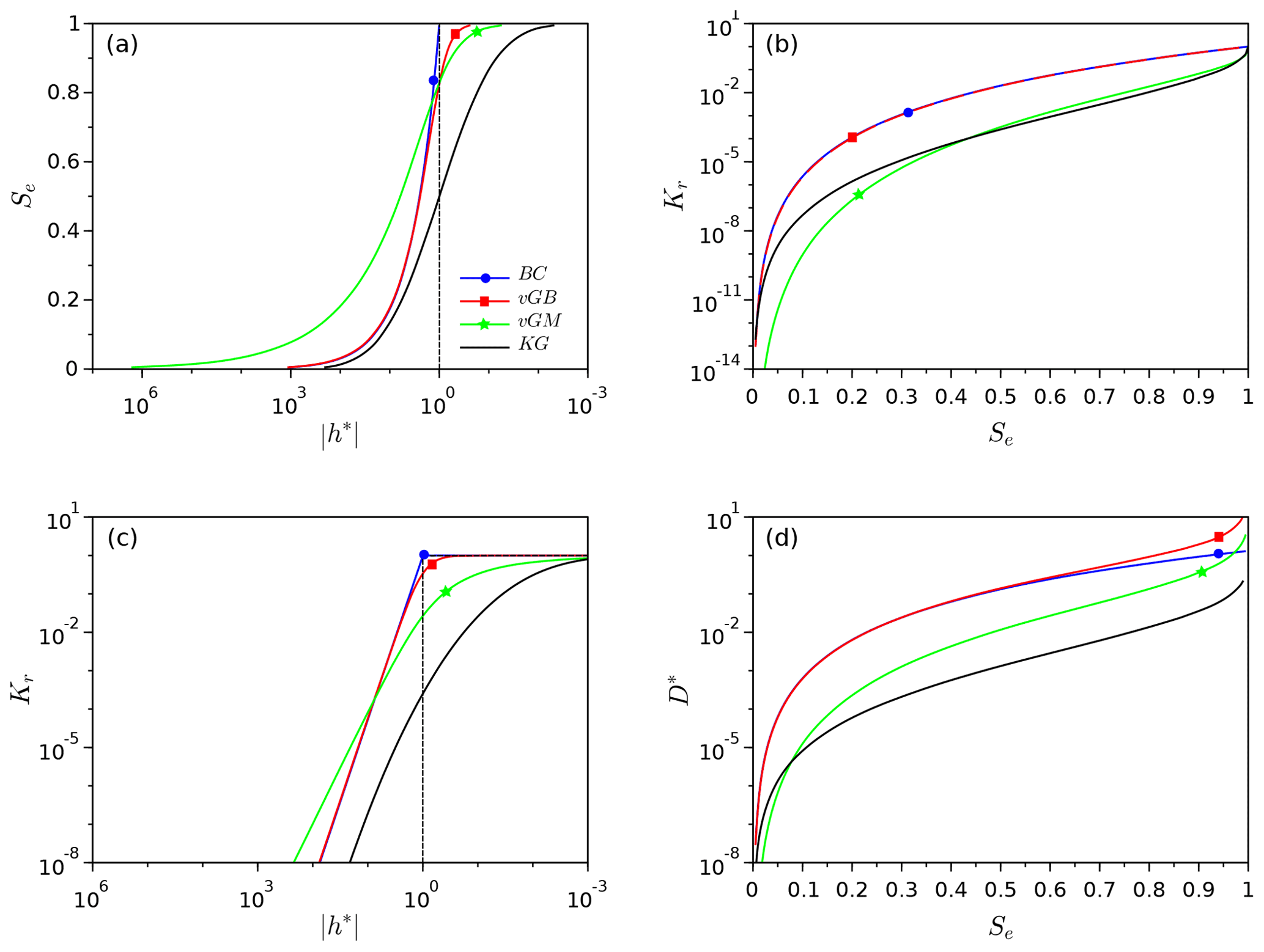
Figure 1Examples of water retention, Se(h*) (a), relative unsaturated hydraulic, Kr(Se) (b) and Kr(h*) (c), and diffusivity D*(Se) functions (d) for the four hydraulic models, Brooks and Corey (BC), van Genuchten–Burdine (vGB), van Genuchten–Mualem (vGM), and Kosugi (KG); the curves were plotted for the same value of the shape index, x=0.275. The hydraulic parameters λBC, mvGM, mvGB, and σKG were computed as a function of x using Eq. (55) with . The dashed line represents the delta model.
The comparison between the hydraulic models (with the same shape index value) reveals some similarities and discrepancies (Fig. 1). Three of the water retention models (vGB, vGM, KG) exhibit an inflection point with a continuous increase in Se(h*) over the whole interval (] (Fig. 1a, vGB, vGM, and KG), while the BC model reaches the asymptote Se=1 at with full saturation for (Fig. 1a, “BC”). Despite that difference, the BC and vGB models exhibit similar shapes (Fig. 1a, BC versus vGB). The vGM model exhibits a more progressive increase in Se(h*) while remaining asymmetrically distributed across the inflection point (Fig. 1a, vGM). Lastly, the KG model exhibits an even more progressive increase and a perfect symmetry around the inflection point (Fig. 1a, KG). The position of the inflection points depends on the chosen hydraulic model. By construction, the inflection point is positioned at for the KG model. The other models have inflection points positioned at larger abscissas (in absolute values), with similar intermediate values for the BC and the vGB models and the largest abscissas for the vGM model (Fig. 1a).
Regarding the relative hydraulic conductivity, the BC and vGB models have similar shapes for Kr(Se), both typical of power functions (Fig. 1b, BC and vGB). In contrast, the vGM and KG models have an inflection point, with a larger increase both at low saturation degrees and close to saturation compared to intermediate saturation degrees. In particular, these two models exhibit a very large increase close to saturation, whereas BC and vGB models have a gradual increase (Fig. 1b, vGM and KG versus BC and vGB, close to Se=1). This feature allows the vGM and KG models to simulate large drops in hydraulic conductivity close to saturation that are typical of certain soils. The functions Kr(h*) are depicted in Fig. 1c and combine the properties of the functions Kr(Se) and Se(h*), as described above. The function Kr(h*) exhibits similar shapes for BC and vGB models, with a quasi-linear and sharp increase for followed by a plateau (Fig. 1c, BC and vGB). The vGM and KG models exhibit a much more progressive increase, involving a much larger range of water pressure heads. This feature is the most pronounced for the KG model. This more progressive increase reflects the more gradual WR functions, Se(h*), as described in Fig. 1a combined with the drop in Kr(Se) that reaches unity only for saturation degrees extremely close to unity (Fig. 1b).
As for the WR and HC functions, the diffusivity functions exhibit close shapes for the BC and vGB models (Fig. 1d). The BC model defines a concave shape with a finite maximum equal to λBC obtained at Se=1, in line with the use of Eq. (38) at Se=1 (Fig. 1d, BC). Conversely, the vGB model diverts from the concave shape to tend towards infinity close to saturation, at Se=1 (Fig. 1d, vGB versus BC). The vGB model defines an S shape that reflects the larger increases at both low and high saturation degrees, with a lower increase at intermediate saturation degrees (Fig. 1d, vGB). The two other models, vGM and KG, exhibit the same type of S shape, with an infinite limit close to saturation (Fig. 1d, vGM and KG). Such an infinite limit spoils the numerical integration of Eq. (22) for the determination of cp, requiring the use of the mixed formulation for the KG models defined by Eqs. (50) and (56).
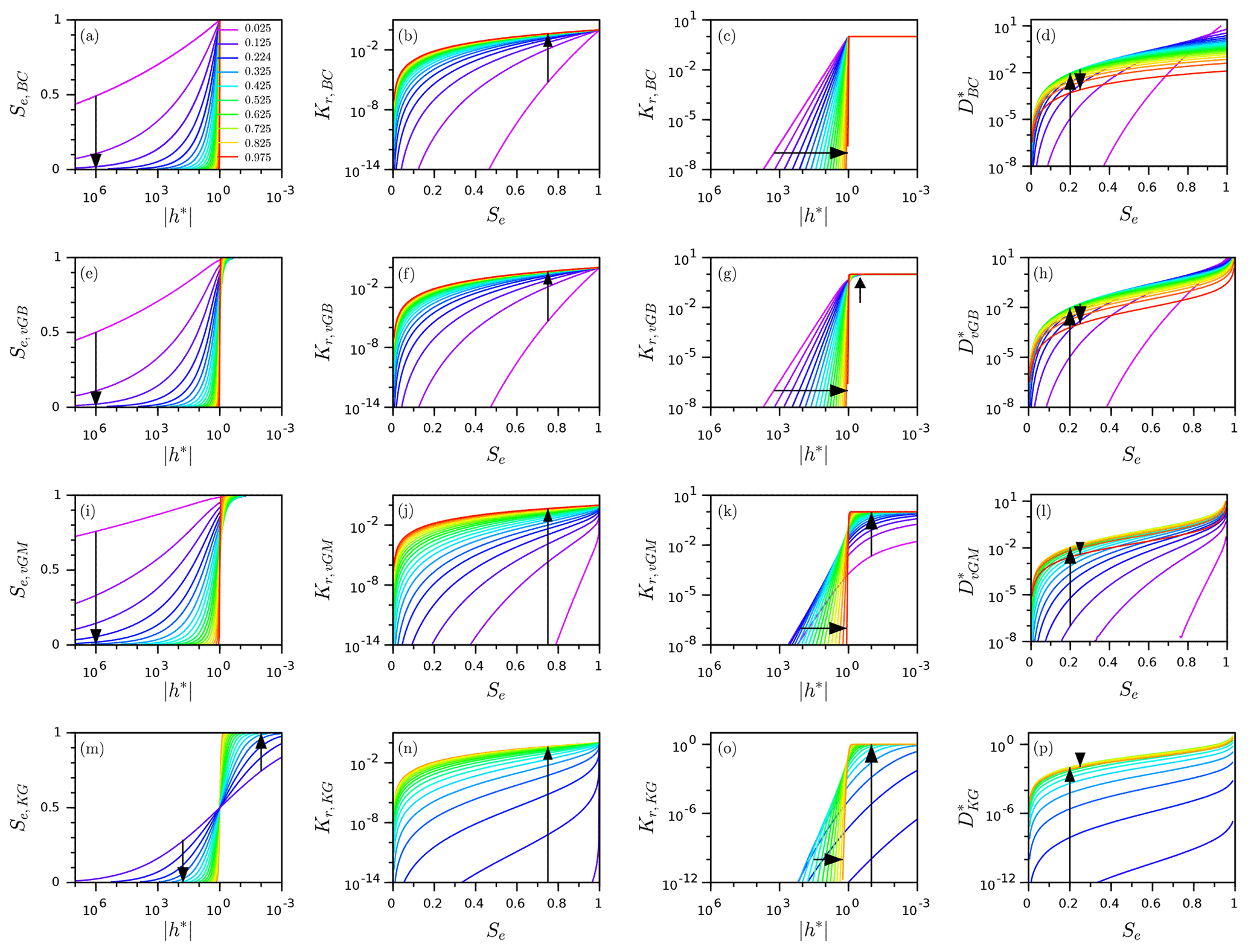
Figure 2Impact of the shape index, x, on the WR and HC functions versus the selected hydraulic models: WR functions, Se(h*) (a, e, i, m); HC functions, Kr(Se) (b, f, j, n) or Kr(h*) (c, g, k, o); and diffusivity function D*(Se) functions (d, h, l, p) for the Brooks and Corey (BC) (a–d); van Genuchten–Burdine (vGB) (e–h); van Genuchten–Mualem (vGM) (i–l); and Kosugi (KG) models (m–p). The arrows indicate increasing values of the shape index x. The hydraulic parameters λBC, mvGM, mvGB, and σKG were computed as a function of x using Eq. (55), with .
Varying the shape index changes the WR and HC functions in an expected way (Fig. 2). For the WR functions, increasing the shape index from 0 to 1 makes the shift from a gradual and moderate to an abrupt increase in saturation degree, respectively. Values close to unity make the WR functions close to a stepwise function correspond to the delta model (Fig. 2, first column, arrows). As for the WR functions, the increase in the shape index puts the curves Kr(h*) close to stepwise functions (Fig. 2, third column, arrows). For the BC model, we notice a decrease in Kr(h*) for , whereas Kr(h*) remains equal to unity above (Fig. 2c, third column). Conversely, for the vGB, vGM, and KG models, the increase in the shape index has two antagonist effects: a decrease of Kr(h*) for , followed by an increase for (Fig. 2g, k, o, third column, arrows). Briefly, as expected, the water retention and the relative hydraulic conductivity tend towards stepwise functions when the shape index tends towards unity (Fig. 2, first and third columns). This trend is less evident for the diffusivity functions (Fig. 2, 4th column).
These results show that, regardless of the model selected, increasing the shape index put the hydraulic functions closer to the delta model that corresponds to soils with narrow pore size distribution. Conversely, very small values of the shape index ensure very gradual shapes for WR and HC functions. However, the results point at contrasting trends when the shape index is decreased towards zero. It is clear that for the vGB and BC models, the relative hydraulic conductivity Kr(h*) is not greatly impacted close to (Fig. 2c and g). Conversely, for the vGM and KG models, Kr(h*) tends towards zero in the vicinity of (Fig. 2k and o, inverted arrows). Similarly, the dimensionless diffusivity, D*(Se), tends towards zero over the whole interval [0,1] when the shape index tends towards zero (Fig. 2l and p, inverted arrows). Consequently, the features of Kr(h*) and D*(Se) functions suggest that the square scaled sorptivity is very small for vGM and KG models, when the shape index tends towards zero (see results below).
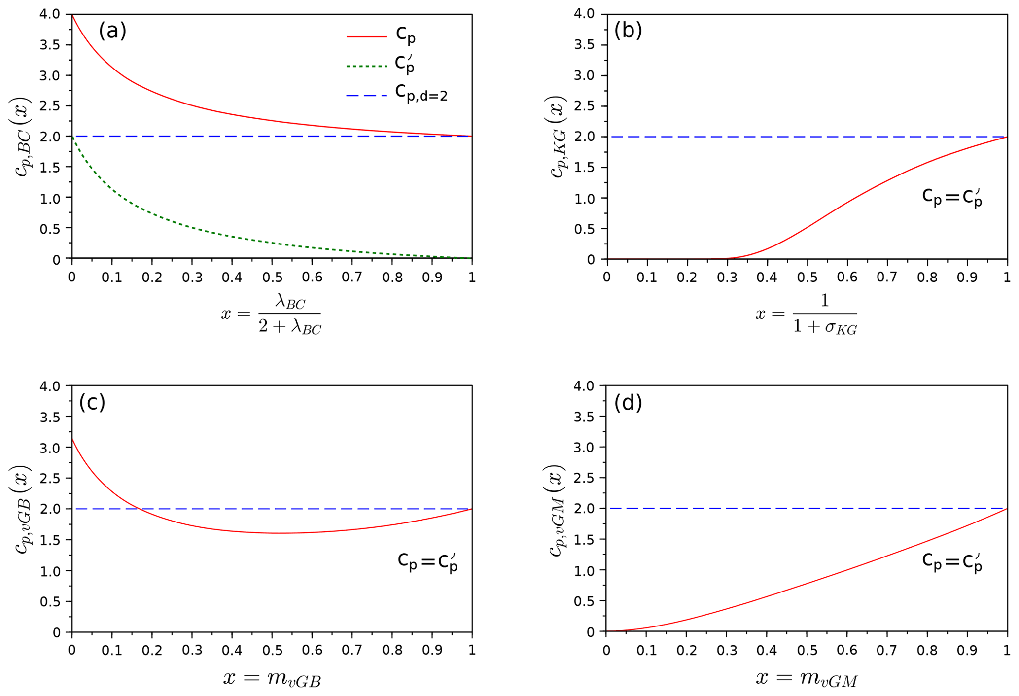
Figure 3Square scaled sorptivity, cp, as a function of shape index, x, for the four hydraulic models, (a) Brooks and Corey (BC), (b) Kosugi (KG), (c) van Genuchten–Burdine (vGB), and (d) van Genuchten–Mualem (vGM); the models were sorted as a function of their monotonic features, with monotonically increasing functions on the right.
3.2 Square scaled sorptivity cp as a function of shape indexes
The square scaled sorptivity, cp(x), is plotted as a function of the shape index, x (Fig. 3). The results show contrasting evolution. For the BC model, we note a decrease of cp,BC(x) from 4 down to 2 (Fig. 3a, cp). Such a decrease is expected since functions decrease over the whole interval (−∞, 0] with the shape index (see Fig. 2c). This leads to the decrease of the integral involved in Eq. (22) and thus cp. The upper and lower limits can be easily determined by applying Eq. (56), leading to and . The air-entry water pressure head is non-null, so that the cp and are related by , since by convention . Consequently, decreases from 2 to 0, with a simple vertical shift compared to cp (Fig. 3a, ). For the other hydraulic models, the air-entry water pressure head is null, so that (Fig. 3b–d). In the following, we compare the evolution of cp as a function of the shape index for each model.
In contrary to the BC model, cp,vGB(x) for the vGB model does not decrease monotonically (Fig. 3c). Instead, cp,vGB(x) decreases to 1.5 before increasing up to 2 for x≥0.52. This feature is in line with the effect of the shape index on the relative hydraulic conductivity, Kr(h*), as described above. The shape index has two antagonist effects: a decrease of Kr(h*) for and an increase for (Fig. 2g, arrows). The numerical computation sorts out these contrasting effects and demonstrates the two-step variation, i.e., a decrease followed by an increase. The two boundaries of the function cp,vGB(x) can be easily found using Eq. (56) with a lower limit of and an upper limit of .
For the KG and vGM models, the trend is opposite, and the functions cp,KG(x) and cp,vGM(x) both increase (Fig 3b and d). This increase is in line with the fact that the shape index mainly increases the diffusivity function, D*(Se), over the whole interval [0, 1] and thus the integral of Eq. (22). The two functions cp,KG(x) and cp,vGM(x) increase from 0 up to 2. For the vGM model, the lower and upper limits can be demonstrated using Eq. (56), leading to (numerical determination) and . For KG hydraulic functions, the lower and upper limits were determined numerically, leading also to 0 and 2, with almost zero values over a large interval of shape index, i.e., (Fig. 3b).
The four functions cp,BC(x), cp,vGB(x), cp,vGM(x), and cp,KG(x) all reach the value of 2 when the shape index approaches unity, i.e., when the WR and HC functions tend towards stepwise functions. In fact, the value of cp(x) converges to the value obtained for the delta model, (see Eq. 42). Such a result indicates that similar results should be obtained for soils with a narrow pore size distribution (like coarse soils with narrow pore size distributions), regardless of the model selected for describing their WR and HC functions. In other words, the choice of the hydraulic model should not matter for soils with narrow pore size distributions. Conversely, contrasting trends are obtained when the shape index tends towards zero: quasi-null values for the vGM and KG models, π for the vGB model, and 4 for the BC model. The null values of cp for the KG and vGB models are in line with the large decrease in D*(Se) over the whole interval [0, 1] when the shape index, x, tends towards zero (see Fig. 2l and p and comments above). Such results show that the choice of the hydraulic model matters for soils with graded pore size distributions. Between these two extreme states, the four functions cp,BC(x), cp,vGB(x), cp,vGM(x), and cp,KG(x) exhibit contrasting evolution, with cp,vGM(x) and cp,KG(x) increasing monotonously, cp,BC(x) decreasing monotonously, and cp,vGB(x) exhibiting a two-step behavior of decreasing followed by increasing values.
This contrasting evolution of functions cp,BC(x), cp,vGB(x), cp,vGM(x), and cp,KG(x) points at different implications regarding the physics of flow and infiltration in soils. It should be borne in mind that the choice of the hydraulic models should not impact the value of the square sorptivity, , for a given soil and given initial conditions, h0. Indeed, sorptivity should be independent of the choice of hydraulic model since it always equals the ratio between the cumulative infiltration and the square root of time for gravity-free infiltration, as illustrated by Eq. (1). However, this work shows that the choice of the hydraulic model strongly impacts the estimation of cp for soils with broad pore size distributions. When the shape index gets close to zero, the BC and vGB models predict non-null values for cp, thus ensuring non-null values of the sorptivity (see Eq. 26), whereas the KG or vGM models predict quasi-null values of cp. We then expect the product of scale parameters, , to compensate for the very low values of cp (see Eq. 26). Given that the scale parameters θs, θr, and Ks characterize dry (residual) or saturated states of the soil, these parameters are not expected to vary between the hydraulic models and are supposed fixed. Consequently, only the scale parameter for the water pressure head, , is expected to compensate for the very low values of cp when the vGM and KG models are used. We conclude that the value of must tends towards being infinite when the shape index tends towards zero for these two models. For the KG model, such a relation, , is related to the relation since . Our statements imply that very large values of σKG(xKG→0) should be associated with very large values of , i.e., with a very small pore radius. In other words, fine (coarse) soils with small (large) pores should have broad (narrow) pore size distributions. These considerations are in line the previous studies on the KG model by Pollacco et al. (2013) (see Fig. 1 of their paper) and Fernández-Gálvez et al. (2019). These authors even related the pore radius of soil to the standard deviation of pore size distribution with a strongly decreasing function. Similar trends relating to some extent a relation between pore mean and pore standard deviation should also apply to the vGM model given our findings (and to avoid null sorptivity for soils with broad pore size distributions). More investigations are needed to verify such a link between average pore size and standard deviation for real soils. More investigations are also needed to guide on the proper choice of the hydraulic models as a function of the soil type, as already suggested by Fuentes et al. (1992). These aspects will be the subject of a specific study.
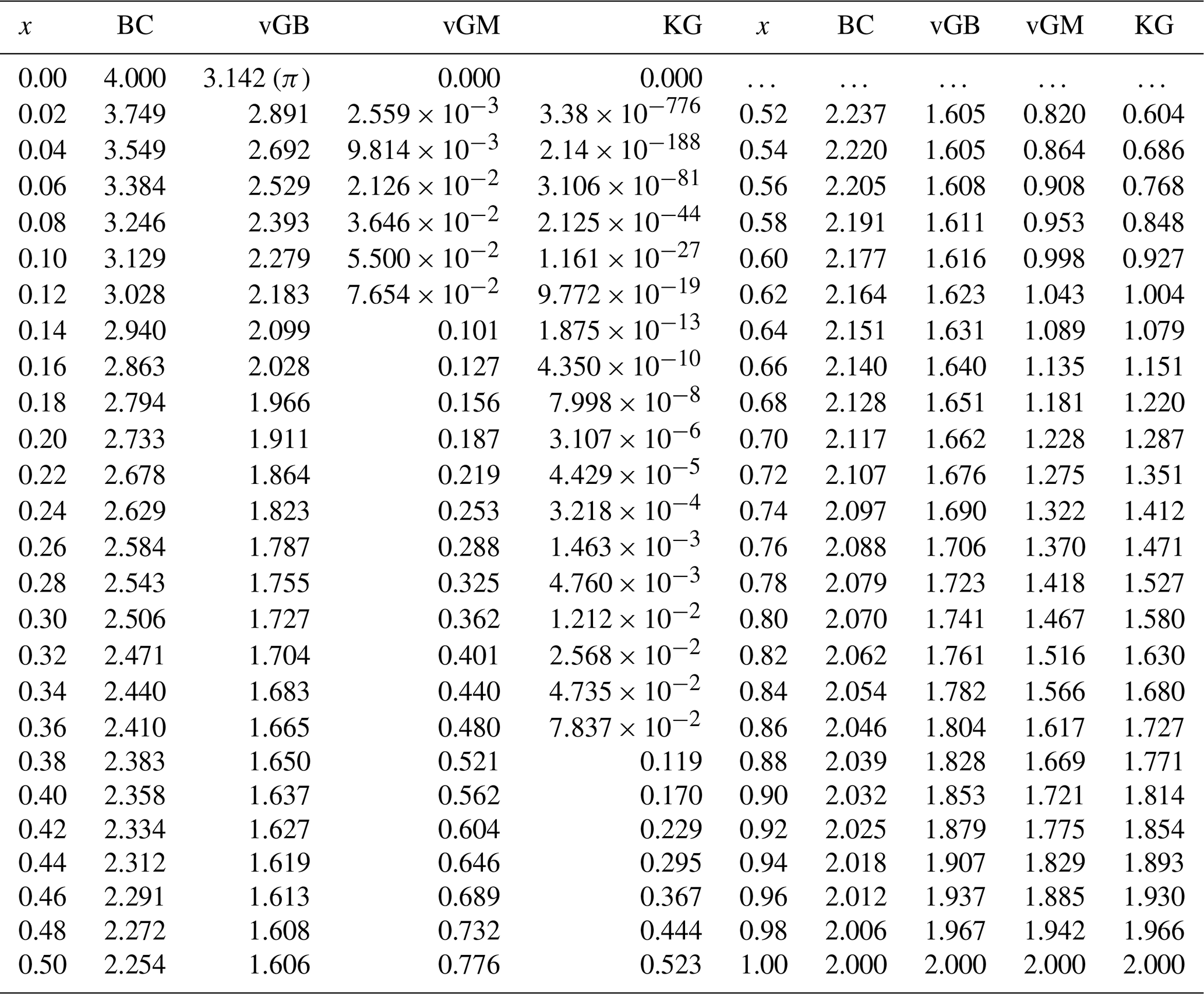
Regarding the numerical accuracy of computed values of cp, we used analytical formulations for the BC, vGB, and vGM models, as detailed in Eq. (56). These values are expected to be perfect without any error since they correspond to the application of exact analytical formulations. Instead, we used the mixed numerical formulation defined by Eq. (50) for the KG model that relies on the numerical integration of the HC or diffusivity functions. In that case, the numerical integration may bring some numerical errors. The mixed form, Eq. (50), was designed to minimize numerical indetermination and uncertainty. Such a formulation was applied to the other models (BC, vGB, and vGM), and the resulting values were compared against the analytical formulations (considered to be the benchmark). A perfect agreement was obtained (errors < 1 %), thus validating the numerical mixed formulation and reinforcing confidence in the values in Table 1. Note that the promotion of the numerical mixed formulation, Eq. (50), and its uncertainty will be the subject of another study.
Table 1Values of the square scaled sorptivity cp as a function of the shape index x for the studied hydraulic models: Brooks and Corey (BC), van Genuchten–Burdine (vGB), van Genuchten–Mualem (vGM), and Kosugi (KG).
3.3 Upscaling sorptivity SK(h0,0) from cp
In this section, we elaborate on the use of Eq. (26) for the easy and straightforward computation of from the tabulated values of cp (Table 1). The proposed scaling procedure Eq. (26) allows for the computation of given initial conditions (water contents or water pressure heads), hydraulic shape and scale parameters, and specific hydraulic models selected among Eqs. (7)–(10):
-
Use the shape parameter (λBC, mvGB, mvGM, or σKG) to compute the related shape index, x, considering the following definitions: xvGB=mvGB, xvGM=mvGM, , and .
-
Choose the value of cp in Table 1 corresponding to the shape index, x, and the chosen WR and HC functions.
-
Consider or compute the initial water content, θ0 or θ(h0), depending on the description of the initial condition (either θ0 or h0).
-
Compute the related hydraulic conductivity, K0=K(θ0), using the HC function.
-
Compute the correcting factors () and (.
-
Compute the scaled air-entry water pressure head, .
-
Compute the square scaled sorptivity, .
-
Upscale to derive the square sorptivity, .
As an illustrative example, let us consider the case of a loamy soil at water saturation with a slightly positive water pressure head at the surface (h1=0) and an initial water pressure head of m (dry conditions). The loamy soil has the features of loam as defined in the database of Carsel and Parrish (1988). Its WR and HC functions are described by the vGM model, with the following shape and scale parameters: θr=0.078, θs=0.43, mm, mm s−1, nvGM=1.56, and lvGM=0.5. The application of the step-by-step procedure gives the following results:
-
shape index: , leading to x=0.359;
-
corresponding value of cp in Table 1 (vGM model column, x=0.36): cp=0.480;
-
initial water content: computed from the initial water pressure head of −10 m using the vGM–WR function, i.e., Eq. (9): θ0=0.125;
-
initial hydraulic conductivity: computed from the initial water content using vGM-HC function, i.e., Eq. (9): mm s−1;
-
corresponding correction factors: and , leading to Rθ=0.865 and RK=1.000;
-
air-entry water pressure head: no air-entry water pressure head, leading to ;
-
square scaled sorptivity: , leading to ;
-
sorptivity: , leading to mm2 s−1 and mm s−½.
To check the accuracy of the proposed approximation, we computed the nominal value of sorptivity, using Eq. (2). We found a very close value, with less than 0.5 % relative error, demonstrating the accuracy of the proposed scaling procedure in Eq. (26).
As a second illustrative example, we consider the computation of sorptivity for the case of the BC model, for the same conditions. The difference with the previous case is that the BC model has a non-null air-entry water pressure head, inducing a non-null saturated sorptivity. We consider the same loamy soil with the following parameters for the BC model: θr=0.078, θs=0.43, mm, and mm s−1, with a value of λBC=0.56. λBC was deduced from the previous value of n=1.56 considering the usual relation λ=mn, as suggested by Haverkamp et al. (2005). The application of the proposed procedure leads to the following computations:
-
shape index: , leading to xBC=0.219;
-
corresponding value of cp in Table 1 (BC model column, xBC=0.22): cp=2.678;
-
initial water content: computed from the initial water pressure head of −10 m using BC-WR function, i.e., Eq. (7): θ0=0.125;
-
initial hydraulic conductivity: computed from the initial water content using BC-HC function, i.e., Eq. (7): mm s−1;
-
corresponding correction factors: and , leading to Rθ=0.866 and RK=1.000;
-
air-entry water pressure head: significant air-entry water pressure head, with hBC=ha, leading to ;
-
square scaled sorptivity: , leading to ;
-
sorptivity: , leading to mm2 s−1, and mm s−½.
Again, the exact value of sorptivity was estimated using Eq. (3) and led to a similar value with a relative error of 1 ‰. Note that, in this case, due to the non-null air-entry water pressure head, Eq. (3) must be employed instead of Eq. (2) for the determination of the targeted value of sorptivity.
The two preceding applications illustrated the accuracy of the proposed scaling procedure, Eq. (26), for both hydraulic functions, with and without air-entry water pressure heads. Equation (26) proved appropriate and very accurate for the determination of the sorptivity, .
It must be noted that the proposed scaling procedure applies only for a dry initial state. Indeed, Haverkamp et al. (2005) stated that their approximation, Eq. (11), was valid only when . For fine soils, even a small initial water pressure head may cause , which may spoil the proposed scaling procedure. To illustrate this point, we investigated the case of silty clay soil, as defined by Carsel and Parrish (1988). This soil is defined with the following parameters: θr=0.07, θs=0.36, mm, mm s−1, n=1.09, and l=0.5. Considering the same value for the initial water pressure head, i.e., m, the initial water content is θ0=0.318, which exceeds . The application of the scaling procedure led to an estimated sorptivity of 0.0475 mm s−½, whereas the targeted sorptivity computed with Eq. (2) was 0.0127 mm s−½. Such an error corresponds to an overestimation by a factor of 2.73. Thus, we advise that the user verify that when θr=0, or more generally before using the proposed scaling procedure.
The proper estimation of sorptivity is crucial to understand and model water infiltration into soils. However, its estimation may be complicated, requiring complicated algebraic derivations and exhibiting potential numerical shortcomings when using Eq. (2) or Eq. (3). In this study, we present a new scaling procedure for simplifying the computation of sorptivity for the case of a zero water pressure head imposed at the surface and dry initial state. We based our approach on the combination and adaptation of the scaling procedure proposed by Ross et al. (1996) and the approximation proposed by Haverkamp et al. (2005). We then obtain a simple relation that relates the square sorptivity to the product of the square scaled sorptivity, referred to as cp, the product of scale parameters, and two correction factors that account for the initial conditions (i.e., initial water content and hydraulic conductivity). The value of the square scaled sorptivity, cp, was computed either analytically, when feasible, or numerically, for four hydraulic models: Brooks and Corey, van Genuchten–Mualem, van-Genuchten–Burdine, and Kosugi models. The values of cp were tabulated as a function of specific shape indexes, representing similar states of WR functions (well-graded versus stepwise shapes) between hydraulic models. The proposed scaling procedure is easy of use, and, given a selected hydraulic model with related hydraulic shape and scale parameters, the following steps are conducted: computation of the shape index from the hydraulic shape parameters, reading of the corresponding value of cp in Table 1, computation of the correction factors (ratios in hydraulic conductivity and water contents, RK and Rθ), computation of the square scaled sorptivity from cp and the correction factors, and, lastly, upscaling by multiplying with the scale parameters. All these steps are easy to conduct and straightforward. Illustrative examples are proposed at the end of this study, and the accuracy of the proposed scaling procedure is clearly demonstrated (with errors less than 1 %), provided that the initial water content fulfills the conditions when θr=0, or more generally .
In addition to providing a straightforward method for the determination of sorptivity, this study brings very interesting findings on the square scaled sorptivity, cp, and its dependency upon the shape index, x, and the chosen hydraulic model. The results show that the function cp(x) strongly depends on the hydraulic model selected for the WR and HC curves. If all the functions cp(x) converge for the same value, i.e., 2, close to x=1 (stepwise WR functions – narrow pore size distribution), they strongly divert close to x=0 (graded WR functions –broad pore size distribution), with values of 0 for vGM and KG models versus 3–4 for the vGB and BC models. However, the sorptivity should remain the same regardless of the selected hydraulic model: one soil under particular initial conditions means one single sorptivity. Consequently, the contrast of scaled sorptivity must be compensated by a contrast in scale parameters. However, among scale parameters, the residual and saturated water contents and the saturated hydraulic conductivity cannot be changed between models, since they characterize the dry and saturated states of the same soil. Consequently, the value of the scale parameter, hg, must be the one to compensate. Previous studies on the Kosugi model have already hypothesized a strong relation between the scale parameter, hKG, and the standard deviation, σKG (Pollacco et al., 2013). In other words, the scale parameter, hKG, should be parametrized as a function of the shape parameter, σKG, to get plausible WR and HC functions and estimates of sorptivity. We may also expect the same link between the scale parameter, hg,vGM, and the shape parameter, mvGM, to avoid unphysical scenarios and null sorptivity. However, such a hypothesis has never been suggested and requires further investigations. These results show the need to better understand the mathematical properties of the hydraulic models, including the links between the hydraulic shape and scale parameters, and to better relate these properties to the physical processes of water infiltration into soils (Fuentes et al., 1992).
In addition to the proposed scaling procedure, this study gave the opportunity to derive the scaled sorptivity analytically for the three models, BC, vGB, and vGM, thus confirming the expressions provided by previous studies. For the vGM model, the analytical derivation is brand new and had never been proposed before. Its use is of great interest and could be implemented into soil hydraulic characterization methods. For instance, additional BEST methods could be developed on the basis of the use of the proposed formulations for the parameter cp to relate sorptivity to shape and scale parameters. In current BEST methods, only the vGB model is considered. The prior estimation of shape parameters allows for the determination of the parameter cp using Eq. (45). Then, the estimation of saturated hydraulic conductivity and sorptivity allows for the determination of scale parameter hg once cp is determined (Lassabatere et al., 2006). A similar procedure may be proposed for the vGM model, using Eq. (49), that relates the parameter cp to the shape parameter mvGM. The development of the BEST method for the specific vGM hydraulic model, that is much more used than the vGB model, will be the subject of further investigations. Another improvement concerns the consideration of the residual water content θr in the proposed scaling procedure. It would also be interesting to somehow derive the residual water content and not to assume it to be equal to zero as it might also alter the shape of the soil water retention function. The use of the scaled sorptivity and the proposed scaling procedure for these purposes is the subject of ongoing studies and will lead to implementations in many methods and tools for the characterization of single- or dual-permeability soils, including the BEST methods (Fernández-Gálvez et al., 2019; Lassabatere et al., 2019) and the SoilWater-ToolBox software developed for the characterization of homogeneous and heterogeneous soils (Fernández-Gálvez et al., 2021).
In the appendices, for the sake of clarity, the notation of the shape parameters was simplified to λ, m, n, σ, in order to avoid heavy equations. The dimensionless diffusivity functions were derived from their definition D*(Se), applying . This task requires us to first derive the inverse functions for the dimensionless water retention curves. The following equations can be easily found through usual algebraic developments:
where erfc−1 is the inverse function of the complementary error function. These functions can be differentiated to define their relative derivatives, :
The differentiation of the function and , considering bijective functions. We also use the usual derivative of the “erf” function, , and the relation between erfc and erf functions, .
The scaled hydraulic conductivity functions are
Note that for the hydraulic conductivity function of the vGM model, Kr,vGM, we distributed the terms according to . The multiplication of Eqs. (A5)–(A8) by the expressions of relative conductivity, Eqs. (A9)–(A12), leads to the following expressions of dimensionless diffusivity:
The expressions in Eq. (A13) correspond to the expressions of Eqs. (33)–(36). Afterwards, the combination with the capillarity model, Eq. (37), leads to Eqs. (38)–(41).
B1 Parameter cp for the BC model
For the BC model, we need to account for the air-entry pressure, . We remind the reader that by convention, the scale parameter for the water pressure head, hBC, is equal to the air-entry water pressure head, ha. We then use Eqs. (22) and (23) with . Then, the first part can be integrated analytically given that the hydraulic diffusivity obeys a power law. The following developments can be done:
The final expression can be easily computed by combining Eqs. (B1) and (B2):
The concatenation of Eq. (B3) with the capillary model, Eq.( 37), leads to the following final expression, assuming p=1:
These development demonstrate the equations proposed for cp for the BC model, i.e., Eqs. (43)–(44). This demonstration is in line with Varado et al. (2006).
B2 Parameter cp for the vGB model
For the vGB model, and the remaining models, there is no air-entry water pressure head, , leading to
Then, the integral can be decomposed into well-known integrals:
The change of variable provides the following expressions:
We now use the beta function B, which has the following properties (assuming x>0 and y>0):
where the Γ function is already defined by Eq. (46): (z>0). Then, the parameter cp,vGB can be expressed as follows:
The last equation uses the fact that . Equation (B9) corresponds to the equation suggested by Haverkamp et al. (2005), considering :
Note that the proposed simplification using the beta function, Eq. (B9), requires that , which is quite evident since m>0. When Eq. (B9) is combined with the capillary model, i.e., Eq. (37), the expression becomes
The expressions of the parameter cp for the vGB model are accurately demonstrated, leading to Eqs. (45) and (47).
B3 Parameter cp for the vGM model
For the vGM model, the same equation, Eq. (B5), applies and can be cut into two parts:
For the sake of clarity, we demonstrate the simplifications of the two terms A and B separately:
The last term of A can be simplified easily:
For the two first terms, we use the same change of variable as above to transform the integrals, leading to
In this case, we need to assume that , i.e. , to use the beta function. Such a condition corresponds to , for the by-default value of . The two first integrals can then be replaced using the beta and the gamma functions, leading to the final expression for part A of cp:
By analogy, the following developments come out for the term B:
The simplification for B is valid as soon as , which is the case since we suppose that . After rearranging terms, the following expressions come out for the scaled sorptivity:
Note that, as stated above, the equation theoretically should apply only for the case of , which is quite restrictive. However, thanks to the analyticity of the functions involved in the expression, this equality remains valid for and can be considered for any value of provided that or . Equation (B19) demonstrates Eq. (48). The combination of these equations with the capillary model Eq. (37) leads to Eq. (49).
Note all computations were done using Scilab free software. The scripts for the computation of Eqs. (28)–(31) for the computation of WR and HC functions, Eqs. (38)–(41) for the computation of the dimensionless diffusivity, and Eqs. (56) for the computation of the cp parameter can be downloaded online at https://doi.org/10.5281/zenodo.4587160 (Lassabatere, 2021). Note also that the computation of the proposed sorptivity was implemented in the SoilWater-ToolBox software that interrelates specific modules to derive the soil hydraulic parameters using a wide range of cost-effective methods, accessible online at https://github.com/manaakiwhenua/SoilWater_ToolBox/ (last access: 7 September 2021, Pollacco and Fernández-Gálvez, 2021) (open source under the GP-3.0 License).
No data sets were used in this article.
LL established the question, performed the analytical developments, computed the numerical results, and provided the first draft of the manuscript. PEP performed the analytical developments and verified the numerical results. DY, BL, DMF, SdP, and MR verified parts of the developments and numerical computations. JP and JFG helped with the use of the Kosugi model. RDS and MAN helped with the editing and the presentation of the results, in particular the writing of the application of the proposed approach for end users. All the authors contributed to the editing of the manuscript.
The authors declare that they have no conflict of interest.
Publisher's note: Copernicus Publications remains neutral with regard to jurisdictional claims in published maps and institutional affiliations.
This research has been supported by the Agence Nationale de la Recherche (grant no. ANR-17-CE04-010).
This paper was edited by Nunzio Romano and reviewed by two anonymous referees.
Angulo-Jaramillo, R., Bagarello, V., Iovino, M., and Lassabatere, L.: Infiltration measurements for soil hydraulic characterization, Infiltration Measurements for Soil Hydraulic Characterization, Springer, https://doi.org/10.1007/978-3-319-31788-5, 2016. a, b, c, d
Angulo-Jaramillo, R., Bagarello, V., Di Prima, S., Gosset, A., Iovino, M., and Lassabatere, L.: Beerkan Estimation of Soil Transfer parameters (BEST) across soils and scales, J. Hydrol., 576, 239–261, https://doi.org/10.1016/j.jhydrol.2019.06.007, 2019. a
Bagarello, V., Di Prima, S., and Iovino, M.: Comparing alternative algorithms to analyze the beerkan infiltration experiment, Soil Sci. Soc. Am. J., 78, 724–736, https://doi.org/10.2136/sssaj2013.06.0231, 2014. a
Braud, I.: Use of scaled forms of the infiltration equation for the estimation of unsaturated soil hydraulic properties (the Beerkan method), Eur. J. Soil Sci., 56, 361–374, https://doi.org/10.1111/j.1365-2389.2004.00660.x, 2005. a
Brooks, R. and Corey, A.: Hydraulic Properties of Porous Media, Hydrology Papers, Colorado State University, Fort Collins, 1964. a, b, c
Carsel, R. F. and Parrish, R. S.: Developing joint probability distributions of soil water retention characteristics, Water Resour. Res., 24, 755–769, https://doi.org/10.1029/WR024i005p00755, 1988. a, b
Cook, F. and Minasny, B.: Sorptivity of Soils, in: Encyclopedia of Earth Sciences Series, Springer, Dordrecht, 824–826, https://doi.org/10.1007/978-90-481-3585-1_161, 2011. a
Fernández-Gálvez, J., Pollacco, J., Lassabatere, L., Angulo-Jaramillo, R., and Carrick, S.: A general Beerkan Estimation of Soil Transfer parameters method predicting hydraulic parameters of any unimodal water retention and hydraulic conductivity curves: Application to the Kosugi soil hydraulic model without using particle size distribution data, Adv. Water Resour., 129, 118–130, 2019. a, b
Fernández-Gálvez, J., Pollacco, J., Lilburne, L., McNeill, S., Carrick, S., Lassabatere, L., and Angulo-Jaramillo, R.: Deriving physical and unique bimodal soil Kosugi hydraulic parameters from inverse modelling, Adv. Water Resour., 153, 103933, https://doi.org/10.1016/j.advwatres.2021.103933, 2021. a
Fuentes, C., Haverkamp, R., and Parlange, J.-Y.: Parameter constraints on closed-form soil water relationships, J. Hydrol., 134, 117–142, 1992. a, b
Haverkamp, R., Leij, F. J., Fuentes, C., Sciortino, A., and Ross, P.: Soil water retention, Soil Sci. Soc. Am. J., 69, 1881–1890, 2005. a, b, c, d, e, f, g, h, i, j, k, l, m, n
Hillel, D.: Environmental soil physics: Fundamentals, applications, and environmental considerations, Academic Press, San Diego, California, 1998. a
Kosugi, K.: Lognormal Distribution Model for Unsaturated Soil Hydraulic Properties, Water Resour. Res., 32, 2697–2703, https://doi.org/10.1029/96WR01776, 1996. a, b, c
Kosugi, K. and Hopmans, J.: Scaling water retention curves for soils with lognormal pore-size distribution, Soil Sci. Soc. Am. J., 62, 1496–1505, 1998. a
Lassabatere, L.: Scilab script for sorptivity, Zenodo [code], https://doi.org/10.5281/zenodo.4587160, 2021. a
Lassabatere, L., Angulo-Jaramillo, R., Soria Ugalde, J. M., Cuenca, R., Braud, I., and Haverkamp, R.: Beerkan estimation of soil transfer parameters through infiltration experiments – BEST, Soil Sci. Soc. Am. J., 70, 521 521–532, https://doi.org/10.2136/sssaj2005.0026, 2006. a, b, c, d, e
Lassabatere, L., Angulo-Jaramillo, R., Soria-Ugalde, J., Šimůnek, J., and Haverkamp, R.: Numerical evaluation of a set of analytical infiltration equations, Water Resour. Res., 45, W12415, https://doi.org/10.1029/2009WR007941, 2009. a
Lassabatere, L., Yilmaz, D., Peyrard, X., Peyneau, P., Lenoir, T., Šimůnek, J., and Angulo-Jaramillo, R.: New analytical model for cumulative infiltration into dual-permeability soils, Vadose Zone J., 13, 1–15, https://doi.org/10.2136/vzj2013.10.0181, 2014. a
Lassabatere, L., Di Prima, S., Bouarafa, S., Iovino, M., Bagarello, V., and Angulo-Jaramillo, R.: BEST-2K Method for Characterizing Dual-Permeability Unsaturated Soils with Ponded and Tension Infiltrometers, Vadose Zone J., 18, 180124, https://doi.org/10.2136/vzj2018.06.0124, 2019. a, b
Mualem, Y.: A new model for predicting the hydraulic conductivity of unsaturated porous media, Water Resour. Res., 12, 513–522, 1976. a, b
Nasta, P., Assouline, S., Gates, J. B., Hopmans, J. W., and Romano, N.: Prediction of unsaturated relative hydraulic conductivity from Kosugi's water retention function, Proced. Environ. Sci., 19, 609–617, 2013. a
Parlange, J.-Y.: On Solving the Flow Equation in Unsaturated Soils by Optimization: Horizontal Infiltration, Soil Sci. Soc. Am. J., 39, 415–418, 1975. a, b
Philip, J. R.: The theory of infiltration: 2. the profile at infinity, Soil Science, 83, 257–264, 1957. a
Pollacco, J., Nasta, P., Soria-Ugalde, J., Angulo-Jaramillo, R., Lassabatere, L., Mohanty, B., and Romano, N.: Reduction of feasible parameter space of the inverted soil hydraulic parameter sets for Kosugi model, Soil Sci., 178, 267–280, https://doi.org/10.1097/SS.0b013e3182a2da21, 2013. a, b
Pollacco, J. A. P. and Fernández-Gálvez, J.: SoilWater-ToolBox, available at: https://github.com/manaakiwhenua/SoilWater_ToolBox.jl, last access: 7 September 2021. a
Ross, P., Haverkamp, R., and Parlange, J.-Y.: Calculating parameters for infiltration equations from soil hydraulic functions, Transp. Porous Media, 24, 315–339, 1996. a, b, c, d, e, f
Šimůnek, J., Jarvis, N. J., van Genuchten, M. T., and Gärdenás, A.: Review and comparison of models for describing non-equilibrium and preferential flow and transport in the vadose zone, J. Hydrol., 272, 14–35, 2003. a, b
Triadis, D. and Broadbridge, P.: The Green–Ampt limit with reference to infiltration coefficients, Water Resour. Res., 48, WR011747, https://doi.org/10.1029/2011WR011747, 2012. a, b, c, d
van Genuchten, M.: A closed-form equation for predicting the hydraulic conductivity of unsaturated soils, Soil Sci. Soc. Am. J., 44, 892–898, 1980. a, b, c
Varado, N., Braud, I., Ross, P. J., and Haverkamp, R.: Assessment of an efficient numerical solution of the 1D Richards' equation on bare soil, J. Hydrol., 323, 244–257, 2006. a, b, c
Yilmaz, D., Lassabatere, L., Angulo-Jaramillo, R., Deneele, D., and Legret, M.: Hydrodynamic characterization of basic oxygen furnace slag through an adapted best method, Vadose Zone J., 9, 107–116, https://doi.org/10.2136/vzj2009.0039, 2010. a, b
- Abstract
- Introduction
- Theory
- Results
- Conclusions
- Appendix A: Dimensionless hydraulic diffusivity functions, D*(Se)
- Appendix B: Analytical developments for the cp parameter
- Code availability
- Data availability
- Author contributions
- Competing interests
- Disclaimer
- Financial support
- Review statement
- References