Evaluating a land surface model at a water-limited site: implications for land surface contributions to droughts and heatwaves

Land surface models underpin coupled climate model projections of droughts and heatwaves. However, the lack of simultaneous observations of individual components of evapotranspiration, concurrent with root-zone soil moisture, has limited previous model evaluations. Here, we use a comprehensive set of observations from a water-limited site in southeastern Australia including both evapotranspiration and soil moisture to a depth of 4.5 m to evaluate the Community Atmosphere-Biosphere Land Exchange (CABLE) land surface model. We demonstrate that alternative process representations within CABLE had the capacity to improve simulated evapotranspiration, but not necessarily soil moisture dynamics–highlighting problems of model evaluations against water fluxes alone. Our best simulation was achieved by resolving a soil evaporation bias, using a more realistic initialisation of the groundwater aquifer state and higher vertical soil resolution informed by observed soil properties, and further calibrating soil hydraulic conductivity. Despite these improvements, the role of the empirical soil moisture stress function in influencing the simulated water fluxes remained important: using a site-calibrated function reduced the soil water stress on plants by 36 % during drought and 23 % at other times. These changes in CABLE not only improve the seasonal cycle of evapotranspiration but also affect the latent and sensible heat fluxes during droughts and heatwaves. The range of parameterisations tested led to differences of ∼150 W m⁻² in the simulated latent heat flux during a heatwave, implying a strong impact of parameterisations on the capacity for evaporative cooling and feedbacks to the boundary layer (when coupled). Overall, our results highlight the opportunity to advance the capability of land surface models to capture water cycle processes, particularly during meteorological extremes, when sufficient observations of both evapotranspiration fluxes and soil moisture profiles are available.

1 Introduction

Droughts and heatwaves can have severe and long-lasting impacts on terrestrial ecosystems (Allen et al., 2015; Reichstein et al., 2013) and humans (Matthews et al., 2017; Pal and Eltahir, 2016). Global climate models are commonly used to project how anthropogenic climate change will affect the magnitude, frequency and intensity of droughts and heatwaves. Heatwaves are projected to increase in the future in response to climate change (Dosio et al., 2018; Zhao and Dai, 2017). The future of droughts is less clear: projections of an increase in future droughts are common in the literature (Ault, 2020), yet regional precipitation projections remain uncertain (Collins et al., 2013) and land surface processes relevant to drought are poorly represented in climate models (Ukkola et al., 2018a).

While there is no universal definition, drought can be classified into meteorological, agricultural, hydrological and socioeconomic drought. From a climate model perspective, drought is an anomalous lack of water at the land–atmosphere interface sustained over time. It begins with a reduction in precipitation (“meteorological” drought), and if this persists it can evolve into “agricultural” drought via low soil moisture or into “hydrological” drought through low streamflow or groundwater (Orth and Destouni, 2018). A critical feedback exists between low soil moisture availability and heatwaves (Seneviratne et al., 2010; Teuling et al., 2010; Vogel et al., 2017). As soil moisture becomes depleted, the surface energy partitioning becomes increasingly dominated by sensible heat fluxes (Q_H) relative to latent heat fluxes (Q_E). This can lead to a positive feedback whereby the high sensible heat fluxes warm the boundary layer, which, combined with the reduced evaporation, leads to increased atmospheric demand for moisture, exacerbating land desiccation (Miralles et al., 2019). A combination of drought and heatwaves leads to wide-ranging impacts on the functioning of terrestrial ecosystems (Reichstein et al., 2013; Schumacher et al., 2019). For example, during the European heatwave and drought in 2003, terrestrial carbon losses of up to 0.5 Pg C were reported, corresponding to roughly 4 years of European terrestrial net carbon uptake (Ciais et al., 2005).

Given projections of worsening heatwaves and potentially more droughts under future climate change, the importance of land surface models (LSMs) to capture land responses and feedbacks to the atmosphere during climate extremes is becoming increasingly recognised (Mazdiyasni and AghaKouchak, 2015; Schumacher et al., 2019; Yang et al., 2019). Despite many improvements to LSMs over the past decades, LSMs have remained poor at simulating water fluxes during water-stressed periods (Egea et al., 2011; De Kauwe et al., 2017; Powell et al., 2013; Trugman et al., 2018; Ukkola et al., 2016a), which likely contributes to biases in land–atmosphere feedbacks during heatwaves (Sippel et al., 2017). LSMs commonly underestimate interannual variations in terrestrial water storage (Humphrey et al., 2018), underestimate Q_E during droughts (Powell et al., 2013; Ukkola et al., 2016a) and lack “persistence” by responding too strongly to short-term precipitation variation (Tallaksen and Stahl, 2014). Poor representation of hydrological processes has been identified as a key reason for model biases. There is uncertainty around soil moisture dynamics, how soil texture information is translated to soil hydraulic properties through pedotransfer functions and how water fluxes are partitioned to different components of evapotranspiration and runoff (Clark et al., 2015; Lian et al., 2018; Van Looy et al., 2017). Various approaches have been adopted to improve LSM hydrology, such as the introduction of groundwater dynamics (Niu et al., 2007), alternative pedotransfer functions (Best et al., 2011) and subgrid-scale processes for runoff generation (Decker, 2015). By contrast, the functions used in LSMs to represent the effect of declining water availability on vegetation function are poorly constrained by data (Medlyn et al., 2016) and not consistently applied. Specifically, some models downregulate the maximum rate of Rubisco carboxylation, whilst others reduce stomatal parameters (De Kauwe et al., 2013). Models also do not account for differences in species-level sensitivity to drought (De Kauwe et al., 2015; Klein, 2014; Zhou et al., 2014). This model gap has driven a significant investment in new theoretical approaches (Dewar et al., 2018; Sperry et al., 2017; Wolf et al., 2016).

Despite model developments, it has remained difficult to disentangle the reasons behind poor model performance due to a lack of suitable observations. Root-zone soil moisture estimates are rare, and, whilst satellite estimates are available, they only cover the top few centimetres or are only available at coarse spatial resolution. Meanwhile, Q_E is routinely measured at the site scale, but gridded large-scale estimates remain highly uncertain (Pan et al., 2020). As such, many past model evaluations have focused on observed Q_H and Q_E from eddy covariance observations (Best et al., 2015) or near-surface soil moisture and evaporation from water balance sites (e.g. Schlosser et al., 2000). However, it is rare for evaluations of LSMs, designed for use in climate models, to utilise observations of soil moisture extending through the root zone with concurrent measurements of water fluxes at high temporal frequency. In this paper, we use a novel dataset from the water-limited Eucalyptus Free-Air CO₂ Enrichment (EucFACE) experiment site in southeastern Australia to evaluate the Community Atmosphere-Biosphere Land Exchange (CABLE) LSM. At this site, frequent measurements of each component of the water balance were made coincident with soil moisture observations to a depth of 4.5 m. The highly variable rainfall at this site leads to extended dry-downs, and the heatwaves in summer commonly exceed 35 ^∘C. We use this high-quality dataset to assess multiple model assumptions commonly used across LSMs within a single model framework, evaluating both simulated fluxes and state variables at seasonal to annual scales and across weather (heatwaves) and climate (drought) phenomena.

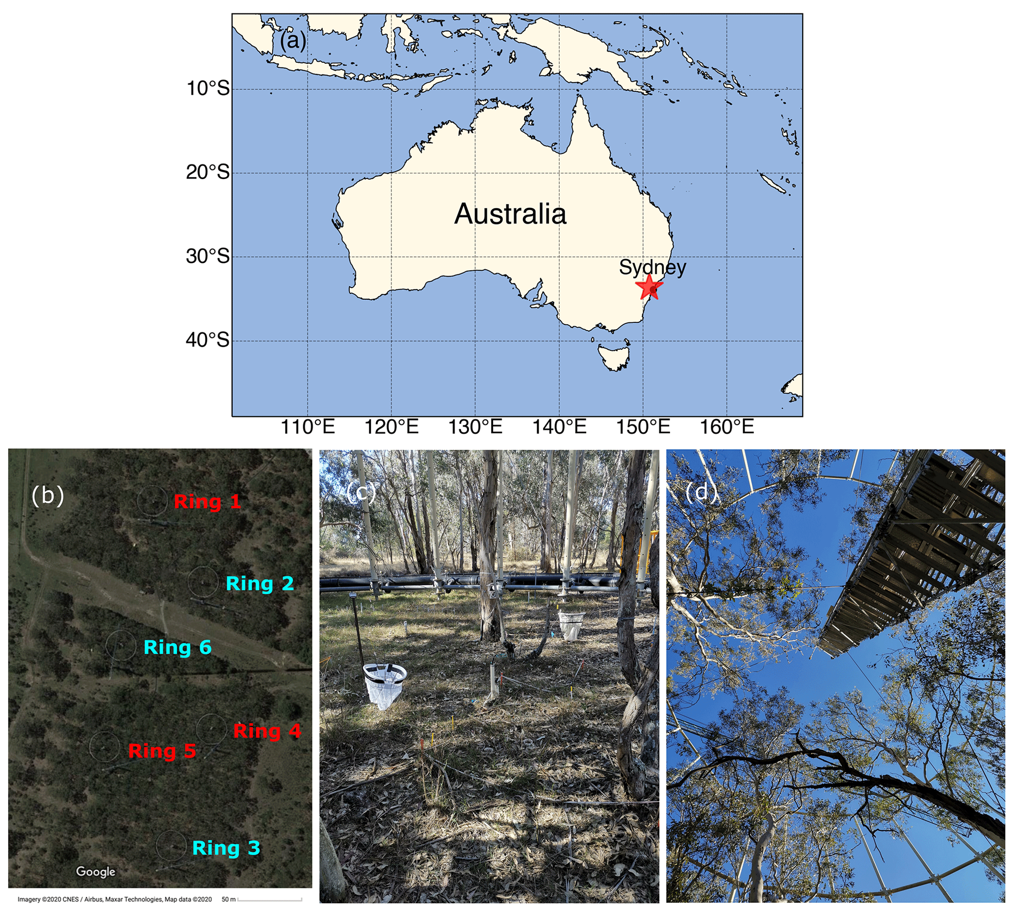
Figure 1 (a) Location of the experimental site in western Sydney, Australia (33^∘36^′59^′′ S, 150^∘44^′17^′′ E) shown by the red star. (b) Distribution of six rings (© Google Maps, 2020, EucFACE experiment site, 1:50, available at: https://www.google.com/maps/@-33.6177915,150.7379194,356m/data=!3m1!1e3, last access: 2 July 2020). (c) Understorey vegetation and infrastructure inside a ring (photograph taken by Mengyuan Mu). (d) Canopy structure and central tower (photograph taken by Mengyuan Mu).

2 Methods and data

2.1 Site information

The EucFACE experiment is located on an ancient alluvial floodplain, 3.6 km from the Hawkesbury River in western Sydney, Australia (33^∘36^′59^′′ S, 150^∘44^′17^′′ E) (Gimeno et al., 2018a; Fig. 1). The site has a temperate–subtropical transitional climate with a mean annual temperature of 17.8 ^∘C and the mean annual precipitation of 719.1 mm evenly distributed over the year. EucFACE is a water-limited site experiencing frequent droughts and low water availability. The site is in an open woodland with a canopy height of 18–23 m and a plant area index (including leaf and woody components) that varied between 1.3 and 2.2 m² m⁻² (mean =1.7 m² m⁻²) over the study period. The overstorey is dominated by a single species, Eucalyptus tereticornis Sm., with scattered individuals of Eucalyptus amplifolia Naudin. The upper soil layer is a loamy sand with a sand fraction >75 %; at 30–80 cm depth, there is a higher clay content layer (15–35 % clay), and below the clay layer sand–clay loam soil extends to a depth of 300 cm. Between 300–350 cm and 450 cm depth, the soil is >40 % clay (Gimeno et al., 2016). The observed water table is at ∼12 m. The site is characterised as nutrient poor, especially lacking in available phosphorus (Crous et al., 2015; Ellsworth et al., 2017). In this paper we evaluate CABLE against the averaged data from rings 2, 3 and 6, which are exposed to the ambient atmospheric CO₂.

2.2 Observation data

In our study, CABLE is driven by in situ meteorological data and observed leaf area index (LAI) from 2013 to 2019. The photosynthetically active radiation (PAR; LI-190, LI-COR, Inc., Lincoln, NE, USA), air temperature and relative humidity (HUMICAP^® HMP 155, Vaisala, Vantaa, Finland) were measured every second, and 1 min averages were recorded on data loggers (CR3000, Campbell Scientific Australia, Townsville, Australia). Following Yang et al. (2020), the meteorological data were gap-filled (0.8 % of values, from 1 January 2013 to 31 December 2019) using linear interpolation, aggregated to 30 min averages and subsequently used to force CABLE at the 30 min resolution. LAI was calculated from the measurements of above- and below-canopy PAR at each ring following Duursma et al. (2016). Since the site LAI represents the plant area index (including both woody part and leaves), to reflect the actual leaves condition we follow Yang et al. (2020) and reduce the LAI by a constant branch and stem cover (0.8 m² m⁻²) estimated by the lowest LAI when the canopy shed almost all leaves during November 2013. The CO₂ concentration was measured every 5 min at each ring and then gap-filled and aggregated to 30 min averages.

To evaluate CABLE, we used measurements of transpiration (E_tr), soil evaporation (E_s) and volumetric water content (θ) at different soil depths (see below). E_tr estimates are derived from tree sap flow velocities (three or four trees per experimental ring) using the heat pulse compensation technique (Gimeno et al., 2018a). Sap flow velocity is translated to E_tr by multiplying the sapwood area estimated from basal area inside each ring and a correlation between sapwood and basal areas based on 35 trees adjacent to the experimental rings. E_s is computed from the soil moisture change in the top 5 cm depth monitored at two locations in each of the three ambient rings. The E_s data also include transpiration from the dynamic (flushes and wilts) understorey vegetation (Collins et al., 2018; Pathare et al., 2017). For E_s, Gimeno et al. (2018a) excluded rainy days and days preceded by a day with >2 mm d⁻¹ of precipitation. To represent variability in E_tr and E_s across rings, we show the mean and the uncertainty within ring estimates in all figures.

We used two sets of observations for θ to evaluate CABLE's simulated soil hydrology. The first dataset is from neutron probe measurements monitored at two locations in each ring every 10 to 21 d (lower frequency in 2017), covering the period January 2013 to July 2019. These data are collected at 12 different depths: 25 cm intervals from 25 to 150 cm depth and 50 cm intervals from 150 to 450 cm depth. The neutron probe counts are converted to θ via the site-specific linear correlation between the raw reading of neutron probe and the lab-measured soil θ sampled at the same depth as probes (Gimeno et al. 2018a). The second dataset is daily derived measurements from frequency-domain reflectometers (CS650, Campbell Scientific Australia, Garbutt, Qld) at each ring, monitoring to a depth of 25 cm and covering the period January 2013 to December 2019.

2.3 Model description

CABLE is a LSM that can be used in stand-alone mode with prescribed meteorological forcing (Haverd et al., 2013; Ukkola et al., 2016b; Yang et al., 2020) or coupled to the Australian Community Climate and Earth System Simulator (ACCESS; Bi et al., 2013; Law et al., 2017) or the Weather and Research Forecasting (WRF) model (Decker et al., 2017; Hirsch et al., 2019b) to provide energy, water and momentum fluxes to the lower atmosphere. The standard version of CABLE has been widely evaluated (De Kauwe et al., 2015; Li et al., 2012; Lorenz et al., 2014; Ukkola et al., 2016b; Wang et al., 2011; Williams et al., 2009), and the model's overall performance in simulating energy, water and energy fluxes is in line with other LSMs (Best et al., 2015). A detailed description of model components can be found in Kowalczyk et al. (2006) and Wang et al. (2011). The version of CABLE used here includes multiple process updates (Decker, 2015; Decker et al., 2017; Kala et al., 2015).

2.3.1 Hydrology scheme

We use the hydrology scheme from Decker (2015) that includes an improved representation of subsurface hydrology similar to that implemented in the Community Land Model (CLM; Lawrence and Chase, 2007; Oleson et al., 2008). Saturation- and infiltration-excess runoff generation mechanisms are represented, and a dynamic groundwater component with aquifer water storage is included. CABLE uses six soil layers covering a depth to 4.6 m and allows for vertical heterogeneity in soil parameters. The scheme solves the vertical redistribution of soil water following the modified Richards equation (Decker and Zeng, 2009):

$$\begin{array}{}\text{(1)}& {\displaystyle \frac{\partial \mathit{\theta }}{\partial t}}=-{\displaystyle \frac{\partial }{\partial z}}K{\displaystyle \frac{\partial }{\partial z}}\left(\mathrm{\Psi }-{\mathrm{\Psi }}_{\mathrm{E}}\right)-F_{\text{soil}},\end{array}$$

where θ is the volumetric water content of the soil (mm³ mm⁻³), K (mm s⁻¹) is the hydraulic conductivity, Ψ (mm) is the soil matric potential, Ψ_E (mm) is the equilibrium soil matric potential, z (mm) is soil depth and F_soil ($\mathrm{mm}{\mathrm{mm}}^{-\mathrm{1}}{\mathrm{s}}^{-\mathrm{1}}$) is the sum of subsurface runoff and E_tr (Decker, 2015). A 22.8 m deep unconfined aquifer is simulated below the six-layer soil column by incorporating a simple water balance model:

$$\begin{array}{}\text{(2)}& {\displaystyle \frac{\mathrm{d}{W}_{\text{aq}}}{\mathrm{d}t}}=q_{\text{re}}-q_{\text{aq,sub}},\end{array}$$

where W_aq (mm) is the mass of water in the aquifer; q_aq,sub (mm s⁻¹) the subsurface runoff removed from the aquifer; and q_re (mm s⁻¹) the water flux between the aquifer and the bottom soil layer, computed by the modified Darcy's law as

$$\begin{array}{}\text{(3)}& q_{\text{re}}=K_{\text{aq}}{\displaystyle \frac{\left({\mathrm{\Psi }}_{\text{aq}}-{\mathrm{\Psi }}_n\right)-\left({\mathrm{\Psi }}_{\mathrm{E},\text{aq}}{\mathrm{\Psi }}_{\mathrm{E},n}\right)}{z_{\text{wtd}}-z_n}},\end{array}$$

where K_aq (mm s⁻¹) is the hydraulic conductivity within the aquifer, Ψ_aq and Ψ_E,aq (mm) are the soil matric potential and the equilibrium soil matric potential for the aquifer, and Ψ_n and Ψ_E,n (mm) are the soil matric potential and the equilibrium soil matric potential for the bottom soil layer. z_wtd and z_n (mm) are the depth of the water table and the lowest soil layer, respectively. The groundwater aquifer is assumed to sit above an impermeable layer of rock, giving a bottom boundary condition of

$$\begin{array}{}\text{(4)}& q_{\text{out}}=\mathrm{0}.\end{array}$$

Subsurface runoff (q_sub, mm s⁻¹) is calculated from

$$\begin{array}{}\text{(5)}& q_{\text{sub}}=\sin \stackrel{\mathrm{‾}}{{\displaystyle \frac{d_z}{d_l}}}{\widehat{q}}_{\text{sub}}{e}^{-\frac{z_{\text{wtd}}}{f_p}},\end{array}$$

where $\stackrel{\mathrm{‾}}{\frac{d_z}{d_l}}$ is the mean subgrid-scale slope, ${\widehat{q}}_{\text{sub}}$ (mm s⁻¹) is the maximum rate of subsurface drainage assumed to be achieved when the whole soil column is saturated and f_p is a tunable parameter. q_sub is generated within the aquifer and for each saturated soil layer below the third soil layer.

2.3.2 Soil evaporation (E_s)

The computation of E_s ($\mathrm{kg}{\mathrm{m}}^{-\mathrm{2}}{\mathrm{s}}^{-\mathrm{1}}$) considers the subgrid-scale soil moisture heterogeneity within a grid square (Decker, 2015) and is given as

$$\begin{array}{}\text{(6)}& E_{\mathrm{s}}=F_{\text{sat}}{E}_{\mathrm{s}}^{\ast }+(\mathrm{1}-F_{\text{sat}}){\mathit{\beta }}_{\mathrm{s}}{E}_{\mathrm{s}}^{\ast },\end{array}$$

where F_sat is the saturated fraction of a grid cell, $E_{\mathrm{s}}^{\ast }$ ($\mathrm{kg}{\mathrm{m}}^{-\mathrm{2}}{\mathrm{s}}^{-\mathrm{1}}$) is the potential evaporation without soil moisture stress and β_s is an empirical soil moisture stress factor (see below) that limits evaporation as water becomes limiting in the top soil layer (Sakaguchi and Zeng, 2009). $E_{\mathrm{s}}^{\ast }$ is given by

$$\begin{array}{}\text{(7)}& E_{\mathrm{s}}^{\ast }={\displaystyle \frac{{\mathit{\rho }}_{\mathrm{a}}\left(q_{\text{sat}}\right(T_{\text{srf}})-q_{\mathrm{a}})}{r_g}},\end{array}$$

where ρ_a (kg m⁻³) is the air density, q_sat(T_srf) (kg kg⁻¹) is the saturated specific humidity at the surface temperature, q_a (kg kg⁻¹) is the specific humidity of the air and r_g (s m⁻¹) is the aerodynamic resistance term.

β_s is computed as

$$\begin{array}{}\text{(8)}& {\mathit{\beta }}_{\mathrm{s}}=\mathrm{0.25}{\left(\mathrm{1}-\cos \left(\mathit{\pi }{\displaystyle \frac{{\mathit{\theta }}_{\text{unsat}}}{{\mathit{\theta }}_{\text{fc}}}}\right)\right)}^{\mathrm{2}},\end{array}$$

where θ_unsat (mm³ mm⁻³) is the volumetric water content in the unsaturated portion of the top soil layer (top 2 cm), and θ_fc (mm³ mm⁻³) is the field capacity in the top soil layer.

2.3.3 Transpiration (E_tr)

CABLE's canopy is represented using a two-leaf model, which computes photosynthesis, stomatal conductance, E_tr ($\mathrm{kg}{\mathrm{m}}^{-\mathrm{2}}{\mathrm{s}}^{-\mathrm{1}}$) and leaf temperature separately for sunlit and shaded leaves. E_tr (for each sunlit and shaded leaf) is calculated following the Penman–Monteith equation:

$$\begin{array}{}\text{(9)}& E_{\text{tr}}={\displaystyle \frac{\mathrm{\Delta }{R}_{{\mathrm{n}}_{\ast }}+C_p{M}_{\mathrm{a}}{D}_{\mathrm{l}}\left(g_{\mathrm{h}}+g_{\mathrm{r}}\right)}{\mathit{\lambda }\left(\mathrm{\Delta }+\mathit{\gamma }\left(\frac{g_{\mathrm{h}}+g_{\mathrm{r}}}{g_{\mathrm{w}}}\right)\right)}},\end{array}$$

where λ (J kg⁻¹) is the latent heat of vaporisation, D_l (Pa) is the vapour pressure deficit at the leaf surface, C_p ($\mathrm{J}{\mathrm{kg}}^{-\mathrm{1}}{\mathrm{K}}^{-\mathrm{1}}$) is the air heat capacity, M_a (kg mol⁻¹) is the molar mass of air, Δ (Pa K⁻¹) is the slope of the curve relating saturation vapour pressure to air temperature and γ (Pa K⁻¹) is the psychrometric constant. g_h, g_r and g_w ($\mathrm{mol}{\mathrm{m}}^{-\mathrm{2}}{\mathrm{s}}^{-\mathrm{1}}$) are the conductances for heat, radiation and water, respectively. $R_{{\mathrm{n}}_{\ast }}$ (W m⁻²) is the non-isothermal net radiation, calculated as

$$\begin{array}{}\text{(10)}& R_{{\mathrm{n}}_{\ast }}=R_{\mathrm{n}}-C_p{M}_{\mathrm{a}}(T_{\mathrm{a}}-T_{\mathrm{l}})g_{\mathrm{r}},\end{array}$$

where R_n (W m⁻²) is the net radiation under isothermal conditions, and T_a and T_l is the air and leaf temperature (K), respectively.

g_w is calculated as

$$\begin{array}{}\text{(11)}& g_{\mathrm{w}}^{-\mathrm{1}}=g_{\mathrm{a}}^{-\mathrm{1}}+g_{\mathrm{b}}^{-\mathrm{1}}+g_{\mathrm{s}}^{-\mathrm{1}},\end{array}$$

where g_a ($\mathrm{mol}{\mathrm{m}}^{-\mathrm{2}}{\mathrm{s}}^{-\mathrm{1}}$) is canopy aerodynamic conductance, and g_b ($\mathrm{mol}{\mathrm{m}}^{-\mathrm{2}}{\mathrm{s}}^{-\mathrm{1}}$) is leaf boundary layer conductance for free and forced convection (Kowalczyk et al., 2006). g_s ($\mathrm{mol}{\mathrm{m}}^{-\mathrm{2}}{\mathrm{s}}^{-\mathrm{1}}$) is the leaf stomatal conductance following Medlyn et al. (2011):

$$\begin{array}{}\text{(12)}& g_{\mathrm{s}}=g_{\mathrm{0}}+\mathrm{1.6}\left(\mathrm{1}+{\displaystyle \frac{g_{\mathrm{1}}\mathit{\beta }}{\sqrt{D_l}}}\right){\displaystyle \frac{A}{C_{\mathrm{s}}}},\end{array}$$

where A ($\mathrm{\mu }\mathrm{mol}{\mathrm{m}}^{-\mathrm{2}}{\mathrm{s}}^{-\mathrm{1}}$) is the photosynthetic rate; C_s (µmol mol⁻¹) is the CO₂ concentration at the leaf surface; β (unitless) is the soil moisture stress factor on plants; and g₀ ($\mathrm{mol}{\mathrm{m}}^{-\mathrm{2}}{\mathrm{s}}^{-\mathrm{1}}$) and g₁ (kPa^0.5) are fitted parameters representing the residual stomatal conductance when A=0 and the sensitivity of conductance to the assimilation rate, respectively. g₁ reflects the plant's water use strategy and was derived for each plant functional type in CABLE (De Kauwe et al., 2015) based on a global synthesis of stomatal behaviour (Lin et al., 2015). β is calculated as

$$\begin{array}{}\text{(13)}& \mathit{\beta }={\sum }_{i=\mathrm{1}}^n{f}_{\text{root},i}{\displaystyle \frac{{\mathit{\theta }}_i-{\mathit{\theta }}_{w,i}}{{\mathit{\theta }}_{f_{\mathrm{c}},i}-{\mathit{\theta }}_{\mathrm{w},i}}},\end{array}$$

where θ_i, ${\mathit{\theta }}_{f_{\mathrm{c}},i}$ and θ_w,i (mm³ mm⁻³) are the soil moisture content, the field capacity and the wilting point for soil layer i, respectively, and f_root,i is the root mass fraction of soil layer i.

CABLE does not have the capacity to simulate interacting water fluxes between the understorey and overstorey vegetation. Instead, it uses a “tiling” approach (fractionally weights separate simulations). As a result, comparisons between CABLE's E_s and data-derived E_s during wetter periods would be expected to be an underestimate as we only consider the fluxes from the overstorey trees. To quantify the effect of the understorey transpiration on the water balance, we also ran an extra simulation for the grass understorey at this site with the same setting as Watr (see below) but using CABLE default grass physiology parameters and a fixed LAI (1 m² m⁻² – site average). The estimated multi-year mean transpiration of 0.94 mm d⁻¹ can be regarded as an upper estimate since the simulation does not consider grass dynamics, overstorey rainfall interception, or water and energy competition between tree and grass. Not accounting for understorey transpiration will lead to an overestimate of moisture availability in the soil profile.

2.4 Experiment design

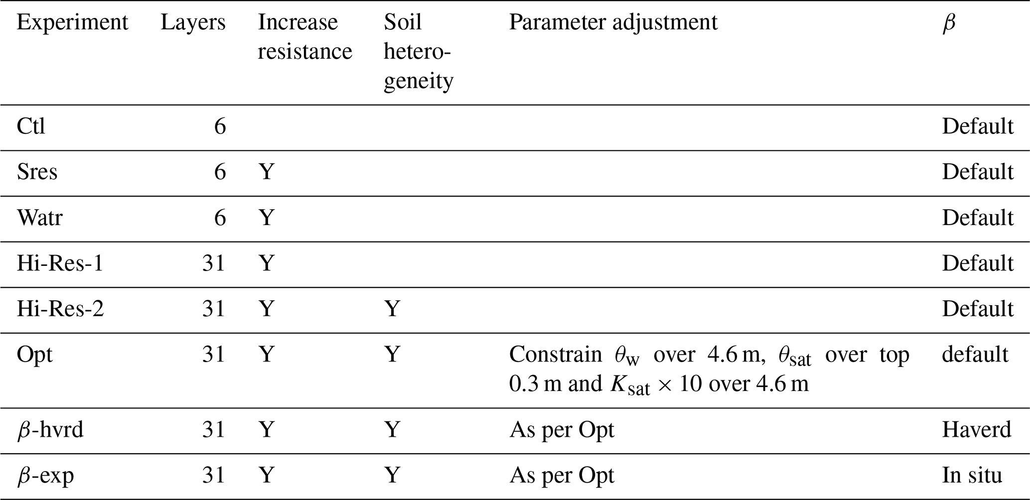
We conducted a series of model experiments based on weaknesses identified in previous LSM evaluation studies. In our experiments, we deliberately adopted a “layering” approach: sequentially resolving a key systematic model bias and then layering additional experiments to examine how much additional benefit each experiment added to model performance. We choose to first resolve a soil evaporation bias as it affects total evapotranspiration (ET) partitioning; however, its importance is limited to the top soil layers, particularly during the period following rain. We then modified the initial water table depth as this fundamentally affects the root-zone soil moisture state. Next, we explored assumptions related to soil column discretisation and parameters, and further optimised key hydraulic parameters to improve overall soil moisture biases. We chose to explore parameter assumptions at this point in the experimental set-up as the previous experiments aimed to resolve existing biases that affected the overall soil moisture availability. Finally, we explored alternative soil moisture stress functions as the last step because this factor integrates, and arises from, the soil moisture state. The experimental order allowed us to probe model biases in a systematic way, but it is important to note that there is no perfect experimental order and alternative permutations would lead to subtly different interpretation of results. In fact, this is what commonly happens in model evaluation that explore a single factor (e.g. the soil moisture stress factor). Each experiment is described in detail below, and a summary of all experiments is provided in Table 1.

Table 1 The experiments conducted. Layers refers to the number of soil layers. Increase resistance refers to increasing surface resistance to soil evaporation. Soil heterogeneity indicates whether soil properties and hydraulic parameters change with depth. The adjustment of θ_w, θ_sat and K_sat and the method used to calculate β are the final two columns.

In all experiments, LAI and physiology parameters were prescribed based on site observations (Table S1 in the Supplement). We tested the difference of using the CABLE default evergreen broadleaf physiology parameters (Fig. S1 in the Supplement) compared to using the site physiology (Fig. 2) and found that using site parameters increases E_tr (due to higher g₁ and increased sensitivity of carbon fixation to temperature), in turn reducing E_s and θ.

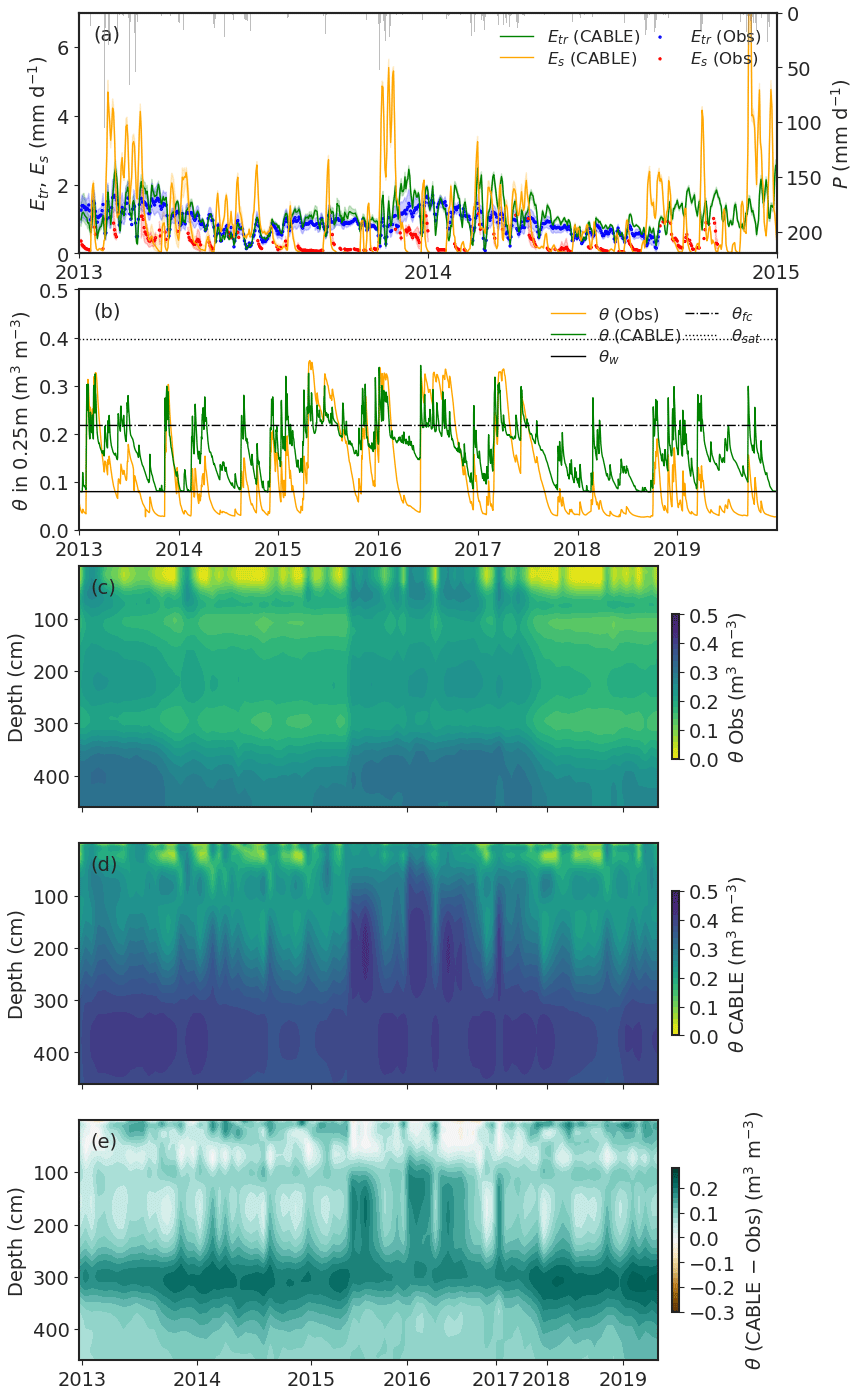
Figure 2 Control simulation (Ctl). (a) E_tr,E_s and precipitation (P) between 2013 and 2015. The shaded areas represent uncertainty between three ambient rings. Both simulations and observations are smoothed with a 3 d window to aid visualisation. (b) θ in the top 0.25 m from 2013 to 2019. (c) The vertical distribution of θ measured at observed dates from 2013 to 2019. (d) The vertical distribution of θ in Ctl for observed dates from 2013 to 2019. (e) θ differences between CABLE and observations. Note the different time axis for panels (c–e) relative to panels (a, b) due to different sampling intervals for soil moisture and fluxes.

All experiments were spun up using an iterative process, recycling all years of the meteorological forcing until the change between two iterations was <0.001 m³ m⁻³ for soil moisture, <0.01 ^∘C for soil temperature and <0.0001 m³ m⁻³ for aquifer moisture.

2.4.1 Control experiment

The control simulation (Ctl) uses the default version of CABLE with six soil layers (but with site-specific physiology and LAI). The soil hydraulic parameters are derived via the pedotransfer functions based on Cosby et al. (1984) using the global soil texture map from the Harmonized World Soil Database (Fischer et al., 2008). Soil parameters are the same throughout the six-layer soil column.

2.4.2 Increasing the resistance for soil evaporation (Sres)

Previous studies suggest LSMs vary widely in their simulation of E_s. For example, De Kauwe et al. (2017) found that, in an ensemble of 10 models, 6 models simulated ∼2–3.5 times more E_s than the other 4 models. LSMs also partition evapotranspiration between E_tr and E_s with a high degree of uncertainty (Lian et al., 2018). At many sites, high springtime evapotranspiration can be linked to excessive E_s rather than E_tr (Decker et al., 2017; Ukkola et al., 2016b) and can lead to biases in soil moisture availability later in the growing season.

We note that models have attempted to resolve this E_s bias through different mechanisms, for example, via a litter layer (Haverd and Cuntz, 2010; Sakaguchi and Zeng, 2009) or by limiting E_s via adding the resistances to vapour diffusion through the soil pores and the surface viscous sublayer (Decker et al., 2017; Haghighi and Or, 2015; Swenson and Lawrence, 2014). Here, we adopt a simple litter layer (Decker et al., 2017) which adds an additional surface resistance to vapour and heat fluxes but does not limit rainfall infiltration. After adding the additional resistance, $E_{\mathrm{s}}^{\ast }$ is calculated as

$$\begin{array}{}\text{(14)}& E_{\mathrm{s}}^{\ast }={\displaystyle \frac{{\mathit{\rho }}_{\mathrm{a}}\left(q_{\text{sat}}\right(T_{\text{srf}})-q_{\mathrm{a}})}{r_g+r_{\text{lit}}}},\end{array}$$

where r_lit is the resistance (s m⁻¹) for diffusion via the litter layer of depth z_l (m) (default value is 10 cm), given by

$$\begin{array}{}\text{(15)}& r_{\text{lit}}={\displaystyle \frac{z_l}{d}},\end{array}$$

where d is the diffusivity of water vapour in air (m² s⁻¹).

2.4.3 Water table initialisation experiment (Watr)

The parameters governing the groundwater aquifer saturation and water table depth are both highly uncertain and difficult to constrain from observations. We investigated the importance of a correct water table depth to the simulation soil moisture and water fluxes. To better match the observed water table depth at EucFACE, we changed the aquifer θ_sat from the model default value (0.235 m³ m⁻³) to θ_sat set based on the observed soil texture at 4.5 m depth (0.448 m³ m⁻³), which reduced the initial saturation of the aquifer from 100 to 52 %. This has the effect of lowering the water table to ∼12 m, in line with observations (Gimeno et al. 2018a).

2.4.4 High-resolution soil experiment (Hi-Res)

Most LSMs assume that soil parameters are depth invariant through the soil profile. The number of layers typically ranges from a minimum of 2 through to 6 in CABLE and up to 20 in the Community Land Model (Lawrence et al., 2019). Here, we test the impact of increasing the number of discrete soil layers, informed by observations of the varying vertical soil texture at the EucFACE site. Recent soil maps (e.g. SoilGrids; Hengl et al., 2017) have begun to capture vertical variations in soil texture, so it is important to test the impact in LSMs.

We performed two sub-experiments in Hi-Res:

1. the number of vertical soil layers was increased from 6 to 31 (to match the resolution of observed soil texture, which was sampled at 15 cm intervals) (Hi-Res-1);

2. soil parameters were allowed to vary vertically based on observed soil texture (Hi-Res-2).

To implement vertically varying soil parameters, the observed fractions of sand, clay and silt; soil bulk density; and organic carbon fraction were taken from measurements at each ambient CO₂ ring and interpolated into 31 layers using the ∼15 cm resolution of the observations. Soil hydraulic parameters are computed using the same pedotransfer functions as used in Ctl but allowed to vary with depth based on the vertical heterogeneity in soil properties. Since CABLE assumes that the Clapp and Hornberger parameter and the parameter for suction at saturation are identical for the aquifer and the bottom soil layer, adding depth-varying soil parameters in Hi-Res-2 also changes these two parameters for the aquifer.

2.4.5 Soil parameter optimisation experiment (Opt)

As it is impractical to measure soil hydraulic parameters at the global scale, pedotransfer functions are used to convert widely measured soil properties into global soil hydraulic parameter datasets (Dai et al., 2013; Kishné et al., 2017). However, most of the widely used pedotransfer functions are empirical equations derived from the limited experimental samples measured for the specific locations (Cosby et al., 1984; van Genuchten, 1980). The adaptability of these pedotransfer functions is always confined by their underrepresentation of some soil properties, such as soil aggregate stability or macroporosity (Puhlmann and von Wilpert, 2012), and can lead to a divergence in model parameters (Van Looy et al., 2017; Zhang and Schaap, 2019). As a result, parameter calibrations are commonly used to obtain more accurate representations.

First, we used the site observations to adjust the plant wilting point (θ_w) and volumetric water content at saturation (θ_sat). With each layer as θ_w is changed, the corresponding residual water content (θ_res) was also updated to ensure it was smaller than θ_w. θ_sat was set to the observed maximum from the daily data measured by frequency-domain reflectometers for the top 30 cm. θ_sat was not adjusted below 30 cm as the observed maximum θ_sat is unlikely to represent saturated conditions due to lower soil moisture variability at depth. θ_w and θ_res were adjusted for each 15 cm layer in the soil column using the observed minimum (OBS_min) in each layer. When OBS_min was below the default θ_res, θ_res was set to OBS_min and θ_w to OBS_min+0.0001 m³ m⁻³. When θ_res <OBS_min <θ_w, θ_w was set to OBS_min. Otherwise θ_res and θ_w were not adjusted.

Second, we optimised K_sat to test whether allowing the soil column to drain faster or slower reduced model biases in the soil moisture profile. K_sat was optimised by concurrently minimising the root mean squared error (RMSE) between modelled and observed transpiration, soil evaporation, and soil moisture over the total column and over the top 0.25 m.

2.4.6 Soil water limitation on transpiration (β-hvrd and β-exp)

LSMs use different empirical functional forms to represent the effect of water stress on vegetation function (see Introduction). To explore the influence of different functional formulations, we compare CABLE's default function (Eq. 13) to two alternative parameterisations: (1) an alternative hypothesis that plants optimise their root water uptake to exploit resources, with the wettest soil layer determining soil water stress on plants (β-hvrd; Haverd et al., 2016) and (2) a site-calibrated function to observations at EucFACE over the top 1.5 m (β-exp; Yang et al., 2020). We note that a number of studies have tested different water stress formulations (e.g. Egea et al., 2011), but this process evaluation is often decoupled from analysis of other contributing errors (e.g. LAI and/or soil hydrology).

The β-hvrd method tends to predict less water stress than the default function (Eq. 13) in CABLE when the moisture is unevenly distributed within the soil column. This function takes the form

$$\begin{array}{}\text{(16)}& \mathit{\beta }=max({\mathit{\alpha }}_i\cdot {\mathit{\delta }}_i,i=\mathrm{1},n),\end{array}$$

where

$$\begin{array}{}\text{(17)}& \mathit{\alpha }=\left\{\begin{array}{ll}{\left(\frac{\mathit{\theta }-{\mathit{\theta }}_{\mathrm{w}}}{{\mathit{\theta }}_{\mathrm{s}}}\right)}^{\mathit{\gamma }/(\mathit{\theta }-{\mathit{\theta }}_{\mathrm{w}})},& (\mathit{\theta }-{\mathit{\theta }}_{\mathrm{w}})>\mathrm{0}\\ \mathrm{0},& (\mathit{\theta }-{\mathit{\theta }}_{\mathrm{w}})\le \mathrm{0}\end{array}\right.,\end{array}$$

where α_i is proportional to the root “shut-down” function (Lai and Katul, 2000) in the ith soil layer, and δ_i=1 if there are roots at the ith soil layer; otherwise δ_i=0. n is the total number of soil layers.

In β-exp, β is an exponential function calibrated to the site observations. Yang et al. (2020) fitted a non-linear relationship between β and θ, based on a fitted exponent term q (0.425, Table S1) using measured soil moisture over the top 1.5 m from EucFACE:

$$\begin{array}{}\text{(18)}& \mathit{\beta }=\sum _{i=\mathrm{1}}^n{f}_{\text{root},i}{\left({\displaystyle \frac{{\mathit{\theta }}_i-{\mathit{\theta }}_{\mathrm{w},i}}{{\mathit{\theta }}_{\text{fc},i}-{\mathit{\theta }}_{\mathrm{w},i}}}\right)}^q.\end{array}$$

2.4.7 Evaluation metrics

We used five metrics to evaluate CABLE's performance compared to observations. RMSE and mean bias error (MBE) were used to evaluate overall performance, and Pearson's correlation coefficient (r) the temporal variability. The absolute differences in modelled and observed 5th (P₅) and 95th (P₉₅) percentile values were used to evaluate the lower and upper tails, respectively. As the observed data have gaps, the metrics were only calculated for days for which observations were available.

3 Results

3.1 Control experiment (Ctl)

We first evaluate the Ctl simulation by comparing to the observed E_tr, E_s and soil moisture (Fig. 2). Overall, CABLE simulates E_tr similarly to the observed E_tr (r=0.85, RMSE = 0.34 mm d⁻¹; Table 2) but overestimates peak E_tr, which is particularly evident in the austral summer of 2014, by 0.54 mm d⁻¹ on average (P₉₅ in Table 2). However, it is worth noting that during the summer of 2014 there was an outbreak of psyllids leading to canopy defoliation (Gherlenda et al., 2016), which may explain part of the model–data mismatch (CABLE only accounts for canopy defoliation via a decline in LAI but not other damage, e.g. to the phloem). Compared to E_tr, CABLE simulates E_s less well (r=0.65, RMSE = 0.70 mm d⁻¹; Table 2, Fig. 2a). Whilst the observations exclude rainy days, when CABLE reaches its highest E_s, CABLE systematically overestimates mean and peak E_s during observed days by 0.12 and 1.22 mm d⁻¹, respectively (MBE and P95 in Table 2). Figure 2b shows that CABLE has a significant wet bias in the top 0.25 m soil moisture and never falls to the observed values below 0.08 m³ m⁻³ during drier periods. Given the excessive E_s (Fig. 2a), the failure of the top 25 cm to dry out is surprising and suggests a parameterisation error and/or the impact of not accounting for understorey transpiration (see Sect. 2). Figure 2e shows that the wet bias in soil moisture is systematic, extending throughout the soil column (particularly between 2.5 and 4.5 m).

Table 2 Performance metrics for the different experiments. Bold numbers are the best value among these experiments.

Taken together, the evaluation of the Ctl simulation implies that a good simulation in one evaporative flux (Fig. 2a) can be achieved for the wrong physical reasons and is associated with major systematic biases in the simulation of near-surface and root-zone soil moisture (Fig. 2b–d).

3.2 Increasing the resistance to soil evaporation experiment (Sres)

Implementing a litter layer (a proxy for additional surface resistance to E_s) in CABLE significantly reduces E_s from 305 mm yr⁻¹ in Ctl to 204 mm yr⁻¹ in Sres (Fig. 3a, Table 3). The simulation of peak E_s is significantly improved compared to Ctl, but CABLE still overestimated E_s (MBE and P₉₅ in Table 2); this is particularly evident during an observed dry period in late 2013. As a consequence of lower E_s compared to Ctl, E_tr is markedly increased (from 341 mm yr⁻¹ in Ctl to 402 mm yr⁻¹ in Sres, Table 3), which implies a reduction in soil moisture stress in the profile (lower β). This degrades the simulated E_tr relative to the observations for all metrics, particularly from around October 2013 to March 2014 (Fig. 3b). With an overall reduction in evapotranspiration, CABLE displays a considerably worse soil moisture profile (cf. Figs. 3c and 2d) and a larger wet bias through most of the soil profile (cf. Figs. 3d and 2e). Thus, resolving the E_s bias alone relocated the bias to other model components, where it was less easily identified using commonly available measurements.

Table 3 Average values from each experiment. Precipitation (P), total evapotranspiration (ET), transpiration (E_tr), soil evaporation (E_s), canopy evaporation (E_c), total runoff (R) including surface and subsurface runoff, soil water drainage to aquifer (D_r), gross primary production (GPP), latent heat (Q_E), sensible heat (Q_H), and volumetric water content in the 4.6m soil column (θ).

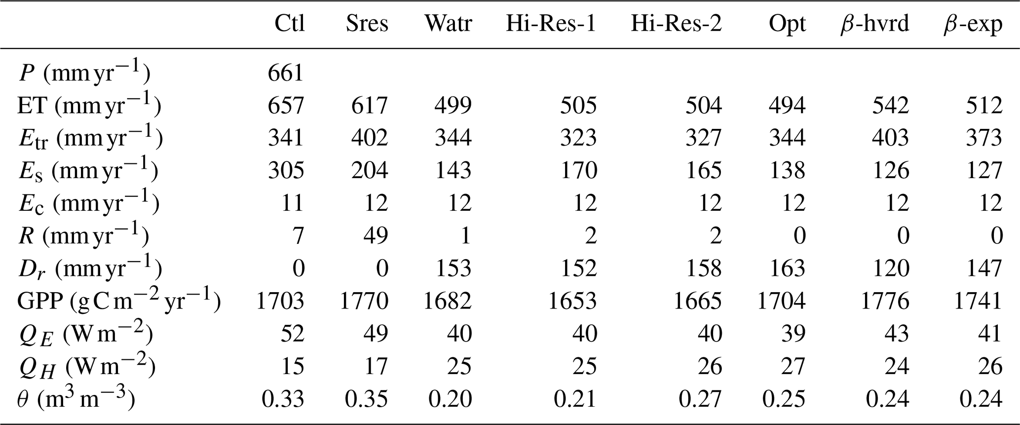
Figure 3 Increasing-soil-evaporation-resistance experiment (Sres). (a) E_s between 2013 and 2015. (b) E_tr between 2013 and 2015. In panel (a) and (b) the shaded areas represent uncertainty between three ambient rings, and both simulations and observations are smoothed with a 3 d window to aid visualisation. (c) The vertical distribution of θ in Sres at observed dates from 2013 to 2019. (d) θ difference between CABLE and observations. Note the different time axis for panels (c, d) relative to panels (a, b) due to different sampling intervals for soil moisture and fluxes.

3.3 Water table (Watr) and vertical soil structure (Hi-Res) experiments

Figure 4 shows that reconciling the parameterisation of the aquifer θ_sat with the bottom layer θ_sat based on observed soil properties (Watr) leads to a marked improvement in the simulated soil moisture profile. By increasing the point of saturation and initialising the aquifer to be drier relative to saturation, CABLE simulates a more negative water potential in the aquifer, which promotes vertical drainage and results in a realistic water table depth in line with observations (simulated and observed ∼12 m over 2013/14). The wet bias in the top 3 m is markedly reduced (cf. Figs. 4d and 2e); however, the model now has a clear dry bias between 3 and 4.6 m. The simulated moisture in the top 0.25 m (Fig. 4b) is now also in better agreement with the observations (0.06 m³ m⁻³ in Watr vs. 0.11 m³ m⁻³ in Sres, MBE in Table S2). Finally, the bias in both the simulated E_s and E_tr is reduced by >0.2 mm d⁻¹ (MBE in Table 2), particularly evident during the summer of 2014.

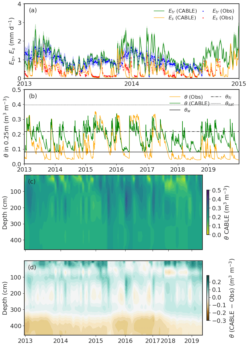
Figure 4 Water table initialisation experiment (Watr). (a) E_tr and E_s between 2013 and 2015. The shaded areas represent uncertainty between three ambient rings. Both simulations and observations are smoothed with a 3 d window to aid visualisation. (b) θ in the top 0.25 m from 2013 to 2019. (c) The vertical distribution of θ in Watr at observed dates from 2013 to 2019. (d) θ difference between CABLE and observations. Note the different time axis for panels (c, d) relative to panels (a, b) due to different sampling intervals for soil moisture and fluxes.

Increasing the number of soil layers from 6 to 31 (Hi-Res-1; Fig. S2) leads to a small improvement in the simulated temporal correlation (0.78 in Watr vs. 0.83 in Hi-Res-1; Table 2) of soil moisture, without notably changing the fluxes. The higher vertical resolution in the soil enables the transition of the dry-down to be better captured, in contrast to the alternating wet and dry patterns associated with the coarse vertical resolution at depths between 0.5 and 3.0 m depth in Watr (cf. Figs. S2c and 4c).

Allowing the soil parameters to vary vertically based on observed soil texture (Hi-Res-2; Fig. 5) reduces the dry bias in the lower layers in Watr (Fig. 4) but leads to a greater wet bias throughout the upper soil profile (<3 m). The error in soil moisture has reduced in the mean, low and high extremes compared to Ctl and Sres (MBE, P₅ and P₉₅ in Table 2). Overall, Fig. 5 highlights a simulation with CABLE where the fluxes of E_tr, E_s and soil moisture are all in reasonable agreement with the observations (Table 3), albeit with an overestimation of peak E_tr.

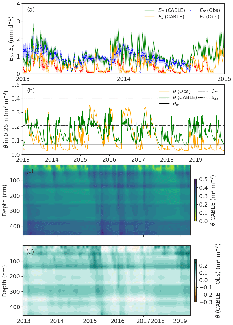
Figure 5 High-soil-resolution experiment (Hi-Res-2), which uses 31 soil layers with depth-varying hydraulic parameters informed by observed soil properties. (a) E_tr and E_s between 2013 and 2015. The shaded areas represent uncertainty between three ambient rings. Both simulations and observations are smoothed with a 3 d window to aid visualisation. (b) θ in the top 0.25 m from 2013 to 2019. (c) The vertical distribution of θ in Hi-Res-2 at observed dates from 2013 to 2019. (d) θ difference between CABLE and observations. Note the different time axis for panels (c–d) relative to panels (a–b) due to different sampling intervals for soil moisture and fluxes.

3.4 Soil parameter optimisation experiment (Opt)

To address the simulated wet bias in the soil moisture profile (Fig. 5), we used observations to prescribe the critical soil hydraulic parameters θ_w and θ_sat (Fig. S3) and to optimise K_sat (Figs. S4 and S5). Prescribing θ_w and θ_sat led to a much improved “operating range” of soil moisture in the top 0.25 cm (Fig. S3b) but did not reduce the wet bias in the soil profile or solve the slow drainage after rainfall events (cf. Figs. 5c and 2c). Overall, these changes had a limited effect on simulated E_tr (344 vs. 327 mm yr⁻¹ in Hi-Res-2 in Table 3) as might be expected because the profile was sufficiently wet as not to limit evapotranspiration, especially in the root zone of the top 1.5 m (Fig. S5d). A reduction of the simulated E_s (138 vs. 165 mm yr⁻¹ in Hi-Res-2; Table 3) was mainly associated with the drier shallow soil (Fig. S5b). The optimised K_sat increased drainage speed (cf. Figs. 5c and 3c) and reduced the overall wet biases (0.04 m³ m⁻³ in Opt vs. 0.07 m³ m⁻³ in Hi-Res-2, MBE in Table 2).

3.5 Soil water limitation on transpiration (β-hvrd and β-exp)

Replacing CABLE's default soil moisture stress function with an alternative hypothesis that plants maximise their root water uptake to exploit resources (β-hvrd) led to a substantial increase in E_tr (Fig. 6a) relative to experiment Opt (from 344 to 403 mm yr⁻¹, Table 3) because the function assumes that the soil water stress on plants is determined by the availability of water in the wettest soil layer. This overestimation of E_tr led to a small reduction in the wet soil moisture bias (cf. Figs. S5d and 6d).

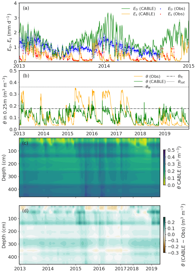
Figure 6 Haverd water stress function experiment (β-hvrd). (a) E_tr and E_s between 2013 and 2015. The shaded areas represent uncertainty between three ambient rings. Both simulations and observations are smoothed with a 3 d window to aid visualisation. (b) θ in the top 0.25 m from 2013 to 2019. (c) The vertical distribution of θ in β-hvrd at observed dates from 2013 to 2019. (d) θ difference between CABLE and observations. Note the different time axis for panels (c, d) relative to panels (a, b) due to different sampling intervals for soil moisture and fluxes.

Figure 7 shows the impact of using a site-calibrated β function (β-exp) (Yang et al., 2020). Using this function also increased E_tr relative to experiment Opt (from 344 to 373 mm yr⁻¹, Table 3), degrading the simulation relative to the standard β (Opt). In both experiments, owing to the overall simulated wet bias in the soil profile, a decreased sensitivity to soil moisture availability (either using β-hvrd or β-exp) did not improve simulated evapotranspiration.

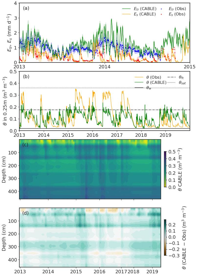
Figure 7 Site-based water stress function experiment (β-exp). (a) E_tr and E_s between 2013 and 2015. The shaded areas represent uncertainty between three ambient rings. Both simulations and observations are smoothed with a 3 d window to aid visualisation. (b) θ in the top 0.25 m from 2013 to 2019. (c) The vertical distribution of θ in β-exp at observed dates from 2013 to 2019. (d) θ difference between CABLE and observations. Note the different time axis for panels (c, d) relative to panels (a, b) due to different sampling intervals for soil moisture and fluxes.

3.6 Implications for drought

Improving the simulation of E_tr, E_s and soil moisture in LSMs is important on the seasonal timescale, but the increasing use of models to simulate future drought highlights the value of examining how these improvements impact the expression of drought in LSMs. We focus on a period of extensive drought across southeastern Australia that begins in October 2017 and extends to the end of 2019. Due to rainfall data availability, we focus on the dry-down period between October 2017 and September 2018.

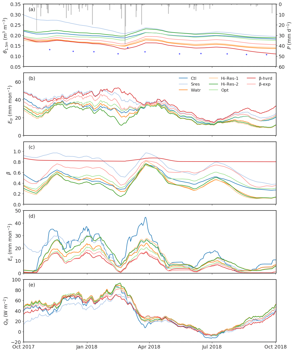
Figure 8 Simulations for each experiment during the drought period (October 2017 to September 2018). (a) The root-zone soil moisture over the top 1.5 m (θ_1.5 m) and rainfall (P; bars), with blue dots showing the observed soil moisture. (b) E_tr, (c) water stress factor (β), (d) E_s and (e) sensible heat (Q_H). All lines are smoothed with a 30 d window.

Figure 8 shows selected fluxes during the drought period, over which the soil slowly dries in the observations and in the models (Fig. 8a) and the shallow soil moisture is close to wilting point (e.g. Fig. 6b). The Sres experiment maintains the highest soil moisture throughout the drought period, and β-hvrd the lowest, with the range across all experiments exceeding 0.1 m³ m⁻³. These soil moisture variations lead to inconsistent behaviour in E_tr (Fig. 8b) due to resulting differences in β (Fig. 8c). β-hvrd E_tr is very high despite having the driest soil moisture (Fig. 8a). Because the calculation uses the wettest soil layer, this leads to notably muted temporal variation (Fig. 8c) relative to the other methods for β. The differences in soil moisture, and as a result β, lead to differences in E_tr (Fig. 8b) of 20–50 mm per month until autumn/winter (∼ April–July), when lower evaporative demand leads to more similar simulations. Through summer (∼ November–February), E_s varies markedly from around 10 mm month⁻¹ (β-hvrd) to 35 mm month⁻¹ (Ctl) (Fig. 8d). The differences in E_tr and E_s are mirrored by differences in Q_H (Fig. 8e), which varies by >30 W m⁻² between the experiments in October 2017 and March 2018.

Integrating the simulations over the drought period highlights the differences in simulating water stress (expressed as β) between experiments. Figure 9a shows that Sres and β-hvrd maintain a relatively high β during drought periods (median >0.7), while the remaining experiments are notably lower. The β-exp simulates median values of 0.63, which is notably higher than the Hi-Res-2 of 0.33 and Opt of 0.46. This difference originates from the calibrated functional form shown in Fig. 9b, where the exponent in the β-exp function leads to a delay in the onset (point of inflection) of moisture stress relative to the default linear function used in CABLE. Overall, in a single model, parameterisations led to a difference of 98 % relative to the averaged median of all the simulations for β simulated during drought.

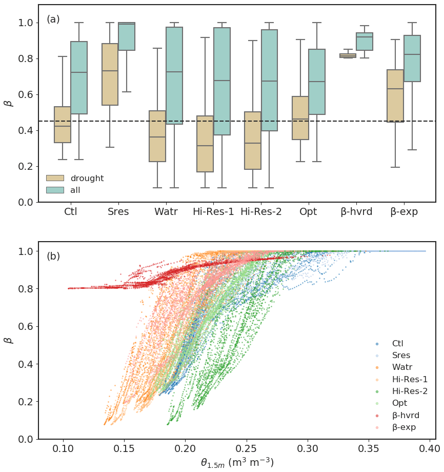
Figure 9 (a) Box plot of simulated β during a drought year (October 2017–September 2018) and all simulated years (2013–2019). The dashed line is the mean value of β in Ctl over the dry period. (b) β variance with root-zone soil moisture over the top 1.5 m (θ_1.5 m) during all simulated years.

3.7 Implications for heatwaves

The link between soil moisture and heatwaves is well known (Teuling et al., 2010) and is usually examined in the context of a drying soil leading to higher Q_H relative to Q_E (as our simulations are uncoupled, we cannot examine the consequences of these changes on the boundary layer).

Figure 10 shows a heatwave that occurred on 19–22 January 2018, where the air temperatures exceeded 35 ^∘C for four consecutive days and exceeded 40 ^∘C on the last day (Fig. 10a). The evaporative fraction during the daytime (09:00–16:00 LT) is shown in Fig. 10b and highlights a remarkable range from ∼0.2 in Ctl to ∼0.7 in β-hvrd, suggesting much stronger evaporative cooling in β-hvrd. An obvious diurnal variation in evaporative fraction is characterised by a progressive decline from a peak at 09:00 LT. Q_E gradually declines through the four heatwave days (Fig. 10c) in all experiments. At the beginning of the heatwave (19 January) daytime Q_E ranges from >200 W m⁻² in β-hvrd and Sres to around 100 W m⁻² in Ctl, Watr, Hi-Res-1, Hi-Res-2 and Opt. The differences in Q_E are mirrored by differences in Q_H (Fig. 10d), with daytime fluxes varying on the heatwave days by more than 150 W m⁻².

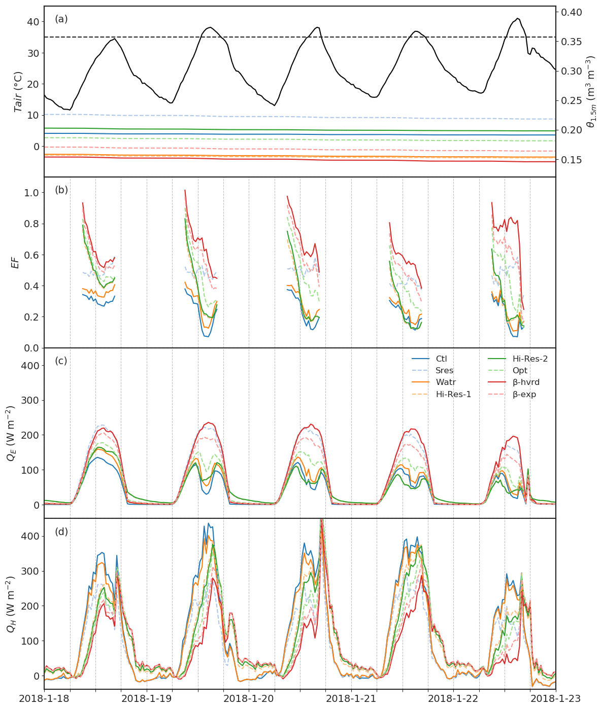
Figure 10 Simulations during an observed heatwave with relatively low soil moisture (19–22 January 2018). (a) Air temperature (T_air; in black) and soil moisture within root zone over the top 1.5 m (θ_1.5 m). The black dashed line shows the 35 ^∘C threshold. (b) Evaporative fraction (EF; calculated for daytime conditions), (c) latent heat (Q_E) and (d) sensible heat (Q_H). The vertical dash lines in panels (b–d) are at a 6 h interval to assist plot reading. One day before the heatwave is also shown.

Figure 10c and d also highlight a key divergence in energy partitioning due to parameterisations and the emergent interactions with soil water availability. Models that show a pronounced midday depression in Q_E (e.g. Ctrl, Watr and Hi-Res-2) due to increasing diurnal vapour pressure deficit (D) and soil moisture stress show earlier diurnal peaks in Q_H (Fig. 10d). By contrast, parameterisations that are less limited by β (e.g. β-hvrd despite the lowest soil moisture, Fig. 10a) see an emergent shift in peak in Q_H to later in the afternoon. When coupled, these emergent differences due to the role of soil water availability – and importantly, how this is translated in canopy gas exchange via β – may have implications for surface interactions with the boundary layer.

Given the importance of the role of D during heat extremes, to further explore the role of high D on simulated E_tr, we plotted modelled and measured transpiration as a function of binned D (Fig. 11). At high D (>2 kPa), simulated E_tr is overestimated. As the mismatch between simulated E_tr and observed occurs at both low and high D (Fig. 11), the model improvements are unlikely to simply relate to an alternative parameterisation of the stomatal sensitivity to D but instead suggest a missing mechanism to limit canopy gas exchange with increasing D. The impact of this overestimation would likely have greater significance for summers with concurrent heatwaves and droughts (compound events that are common in Australia), as during heatwaves when D is higher the model would overestimate E_tr, using up available soil moisture.

Figure 11 Modelled hourly E_tr compared with measured hourly E_tr over 2013. The solid line represents the 1:1 line. The dashed line is the linear fit between modelled and measured E_tr. Colours of dots indicate the range of vapour pressure deficit.

4 Discussion and conclusions

Land surface schemes used in climate models range in complexity, and different approaches translate into contrasting predictions of the exchange of carbon, energy and water (Fisher and Koven, 2020). Perhaps critically, how strongly the land is coupled to the atmosphere also varies widely and is typically attributed to soil moisture variability (Brantley et al., 2017; Dirmeyer, 2011; Guo et al., 2006). A key component of LSMs is how soil moisture availability impacts processes internal to the land model and, in turn, how these impact fluxes of carbon and water. In this paper we used a rich observational dataset from a water-limited site that experiences both high temperatures and pronounced periods of low rainfall to explore a range of alternative model-based assumptions at multiple timescales (daily to annual) within a single model framework. We focused on the capacity of the model to simulate both the state (soil moisture) and the fluxes (evapotranspiration and its components) at a water-limited site. Whilst our analysis is site specific, the issues indicated here have been reported to lead to systematic biases in LSMs across multiple sites (Ukkola et al., 2016a; Trugman et al., 2018). We demonstrated that the default simulation (Ctl, Fig. 2) was able to simulate good transpiration fluxes but for the wrong reasons: erroneously high soil evaporation with a marked wet soil moisture bias. Errors of this kind may not have been identified in previous LSM evaluations against eddy covariance data which mostly focus on Q_E (Best et al., 2015). Our results highlight a potential bias in model evaluations due to a limited capacity to assess soil moisture or the partitioning of evapotranspiration. We demonstrated that poor model behaviour could be overcome via four key steps: (i) reducing soil evaporation biases, (ii) correctly initialising the aquifer moisture content, (iii) adjusting soil parameters to match site conditions and (iv) replacing the function used to constrain transpiration as soil moisture becomes limiting. Since our study attempts to articulate the common issues in the simulated dry conditions in LSMs, we anticipate our findings would be applicable not only in many water-limited conditions but, equally, in more mesic systems too.

Given the critical role of drought-prone ecosystems in contributing to interannual variability in the land CO₂ sink size (Ahlström et al., 2015), our approach has the potential to improve the representation of these systems in models. We note that despite these improvements we still simulated a persistent wet soil moisture bias (e.g. Fig. 5d). We think on balance this is unlikely to originate from not simulating a seasonal understorey transpiration as β-hvrd, which grossly overestimated overstorey transpiration and did not sufficiently dry out the profile (cf. Figs. S5d and 6d). Instead the soil moisture bias must relate to CABLE's representation of subsurface processes.

4.1 Soil evaporation

LSMs commonly overestimate soil evaporation especially under a sparse canopy or over bare land (De Kauwe et al., 2017; Swenson and Lawrence, 2014), suggesting this is a key model weakness. Errors in soil evaporation are rarely isolated in models and often contribute to errors in transpiration by limiting soil moisture availability later in the growing season (Ukkola et al., 2016b) as well as affecting the distribution of shallow versus deep soil moisture draw-down during drought. Here we used a simple approach that increased resistance to surface evaporation, approximating the role of surface litter (Decker et al., 2017). At this site, this increased resistance to surface evaporation improved agreement with observations (Sres; Fig. 3a) but did not resolve all biases. Notably, soil evaporation was not directly measured at the site, but instead derived from the change in observed soil moisture over the top 5 cm, while ignoring days following rain (when the soil evaporative flux would likely be largest) (Gimeno et al., 2018a). As such, it contains soil moisture changes due to transpiration from a seasonal grass understorey but ignores evaporation below the top 5 cm, complicating model evaluation. Nevertheless, the magnitude of CABLE biases points to systematic errors in soil evaporation that do not merely arise form observational uncertainty. Many soil evaporation schemes used in LSMs lack a physical basis, estimating soil evaporation from aerodynamic resistance and an empirical soil water stress and ignoring the role of soil pores. However, a number of studies using alternative process-based schemes have been shown to improve individual model simulations (Haverd and Cuntz, 2010; Lehmann et al., 2018; Or and Lehmann, 2019). For example, Swenson and Lawrence (2014) introduced a dry-surface-layer-based soil evaporation resistance into CLM to depict water diffusion from dry soil, reducing biases in evapotranspiration and total water storage relative to FLUXNET-MTE and GRACE datasets. Based on a pore-scale model (Haghighi and Or, 2015), Decker et al. (2017) added the resistances of capillary–viscous and boundary layer to the CABLE soil evaporation scheme, lowered the positive E_s bias in springtime and improved seasonality of evapotranspiration. Hence, a focused intercomparison of competing approaches against data originating from different ecosystems would be a valuable area of future work.

4.2 Aquifer initialisation

Our results showed that the initialisation of the aquifer moisture store was critical to an improved simulation of the soil moisture profile. By default, CABLE equilibrates the aquifer state by assuming almost complete saturation at the start. If, as happened with the Ctl, the aquifer is initialised too wet, the simulated water table is too high and the water potential in the aquifer is unlikely to be below the lowest soil moisture layer, impeding vertical aquifer recharge. When we initialised from a drier starting position (Watr), the simulated soil moisture profile matched the observed better, with implications for other models using similar groundwater schemes (e.g. CLM4.5, Noah-MP, JULES and LEAFHYDRO). First, our results imply that LSMs that incorporate groundwater schemes need to be careful about aquifer initialisation because this strongly affects soil moisture dynamics. Second, there is no obvious solution to this initialisation and spin-up problem because drainage into the aquifer is a slow process, and it may take hundreds of years to reach a realistic equilibrium state. For global simulations, this suggests the need to a priori initialise the starting aquifer state and to assess against satellite-based products like GRACE (Döll et al., 2014; Niu et al., 2007) or implement offline spin-up using meteorological forcing consistent with the subsequent simulations. However, while spin-up with observations is attractive, when the resulting states are incorporated into a coupled global model, inconsistencies are inevitable. Third, CABLE currently assumes a spin-up approach for the aquifer identical to that of the soil moisture, iterating until state changes between sequences of years are smaller than some threshold. LSMs that employ similar iteration approaches (Gilbert et al., 2017) are likely to encounter similar problems to CABLE because the rate of drainage into the aquifer is very slow, leading to negligible changes between iterations and thus satisfying the criteria for equilibrium.

4.3 Soil layers and pedotransfer functions

LSMs typically define a fixed number of soil layers globally, anywhere up to 20 layers. Most LSMs assume constant parameters across the entire soil profile, either using an experimental look-up table based on soil classification or estimating parameters from empirical pedotransfer functions. We explored the implications of these assumptions by first increasing the number of soil layers to match the number of observed layers (Hi-Res-1; Fig. S2) and then implementing soil parameters that varied vertically based on site texture (Hi-Res-2; Fig. 5). Increasing the vertical resolution had a small impact on the soil moisture and fluxes but did improve the temporal variability in soil moisture compared to observations. The use of site soil texture better depicts the moisture distribution in the soil profile but led to a slightly degraded soil moisture simulation. These results again highlight uncertainties in the translation of soil texture information to hydraulic parameters for water retention and hydraulic conductivity via the empirical functions, which are derived from limited observations (Van Looy et al., 2017). The development in pedotransfer functions via machine learning or multi-model ensemble provides new avenues to reduce errors from parameters (Zhang and Schaap, 2017; Dai et al., 2019). High-resolution global soil datasets (e.g. SoilGrids, Hengl et al., 2017) covering multiple soil layers up to 2 m depth offer opportunities to improve LSM simulations of soil moisture by incorporating depth-varying soil parameters. It is noteworthy that these global datasets of soil hydraulic parameters (Montzka et al, 2017; Dai et al., 2019) have existed for several years but have not been widely used. Furthermore, at the EucFACE site, the observed soil texture information enabled the separation of parameter uncertainties from biases in process representations and model structural errors, a valuable step in better constraining LSM simulations.

4.4 Calibration of soil hydraulic parameters

A number of studies have used satellite-derived (passive and active microwave) estimates of soil moisture to optimise soil hydraulic parameters in the top few soil layers (Harrison et al., 2012). Clearly these approaches are a potential way to constrain LSMs globally given the plethora of satellite observations extending back to the 1970s. However, these approaches implicitly assume that improving near-surface soil moisture translates to improvements over the entire soil column, an assumption not supported by our results. Whilst the use of observation-constrained θ_w and θ_sat over the top 0.3 m improved the simulated dynamics of shallow soil, it did not result in a large reduction in the bias simulated in deeper soil moisture layers (Fig. S3). At this site, the inability to significantly improve soil moisture dynamics through calibration of soil hydraulic conductivity against observed soil moisture data likely relates to the complexity of the soil profile, which contains two clay layers at depth (30–80 and 300–450 cm). This vertical texture complexity meant that it was difficult to obtain unique parameter solutions that would sufficiently improve vertical drainage whilst simultaneously simulating moisture dynamics well (Fig. S5). On the other hand, the neutron probe measurements of soil moisture used for calibration also involve uncertainties (Gimeno et al. 2018a). The soil moisture estimates were derived by fitting two distinctive linear relationships between soil volumetric water content and raw neutron probe counts (see Fig. S6) for clay (below 3 m) and non-clay soil (above 3 m). As a result, the observation error would be greatest in layers where the soil type differs from the assumed soil type at that depth. However, the fitted relationships were robust, since clay soils largely dominated the deeper profile (below 3 m depth) and sand soils mostly dominated the shallow profile (above 3 m depth). Overall, our sensitivity experiments suggest that optimising soil properties alone is not sufficient, and calibration exercises should also account for vegetation information to reduce biases in subsurface processes.

4.5 Water stress functions

Studies commonly highlight the functions used to limit photosynthesis and stomatal conductance with water stress as a key weakness among models. The lack of theory in this space (Medlyn et al., 2016) has led to models employing a range of functions encompassing different shapes and sensitivities that are not constrained by data. Trugman et al. (2018) explored the role of soil moisture stress in simulated “potential” gross primary productivity (GPP) among CMIP5 models and argued that the functional form used to represent the effect of soil moisture stress was the major driver of carbon cycle uncertainty. Here we deliberately attempted to first resolve model biases through other avenues (e.g. soil evaporation, soil parameterisation), because it is likely that model biases originate from multiple sources (e.g. leaf area, soil moisture dynamics etc.). We were subsequently able to assess the capacity to then further improve model behaviour via the functional forms used to represent water stress.

We examined three alternative water stress functions: the linear θ-based function used in Ctl (common among models, e.g. SDGVM, Orchidee-CN and JULES), a non-linear θ-based β (β-exp) calibrated for this site from Yang et al. (2020) and a function based on Haverd et al. (2016) (β-hvrd). Haverd et al. (2016) hypothesised that plants optimise their root water uptake, only limiting function when water in the deepest accessible soil layer becomes limiting. They further argued that this behaviour did not vary among sites (and so species). De Kauwe et al. (2015) previously tested this hypothesis and demonstrated that it led to an underestimation of the effect of moisture stress, inconsistent with observations. Our results again show that this hypothesis is not supported by data and led to an overestimation of transpiration (Fig. 6) and little evidence of moisture stress (Fig. 9b). We found that, after reducing other model biases, the use of the calibrated β−exp function did reduce the simulated soil moisture stress (over the drought year, median β=0.63 vs. 0.33 in Hi-Res-2 and 0.46 in Opt; Fig. 9). Overall, the various experiments show markedly different median β (ranging from 0.67 to 0.99, considering all simulated years), consistent with previous evaluations that have highlighted differences in simulated β across models (De Kauwe et al., 2017; Medlyn et al., 2016; Powell et al., 2013; Trugman et al., 2018). However, our results highlight that differences originate as much from alternative model assumptions and biases (e.g. soil evaporation, soil parameters) as the functional forms themselves. Alternatives to the β functions have emerged to fill the theoretical gap, including plant hydraulic (Christoffersen et al., 2016; Xu et al., 2016) and stomatal optimality approaches (Sperry et al., 2017), but are yet to be widely adopted in LSMs (but see Eller et al., 2020; De Kauwe et al., 2020; Kennedy et al., 2019; Sabot et al., 2020). Replacing the empirical soil water stress factor by these plant physiology schemes reduces model arbitrariness associated with the representation of soil water stress and reduces the simulated biases in transpiration either over water deficit regions or in areas with obvious dry seasons (Bonan et al., 2014; De Kauwe et al., 2020; Sabot et al., 2020). We can envision that a wider application of these processes-based models will offer a chance to improve water stress representation in more LSMs.

4.6 Heatwaves

Differences between the versions of CABLE lead to a different initial soil moisture state at the beginning of a heatwave, ranging from ∼0.15 m³ m⁻³ (β-hvrd) to ∼0.23 m³ m⁻³ (Sres) (Fig. 10). In addition to the impact of the initial state, differences between parameterisation also affect estimates of β, leading to large divergences in evaporative cooling during a heatwave. Consequently, some versions of CABLE respond to the heatwave with a reduction of Q_E and a higher Q_H during 12:00–16:00 LT, while other simulations maintain a high Q_E during this period and the high Q_H shifts to later afternoon (16:00–18:00 LT) (Fig. 10c and d). The magnitudes of Q_E and Q_H between simulations are also substantially different: Ctl would amplify a heatwave, warming and drying the boundary layer, while β-hvrd would tend to moisten and (relatively) cool the boundary layer. Many studies have shown that the land surface can play a key role in amplifying heatwaves (Hirsch et al., 2019a; Miralles et al., 2014; Teuling et al., 2010), and LSMs exhibit systematic biases in representing this feedback (Sippel et al., 2017; Ukkola et al., 2018b). For a mega-heatwave like the 2010 European heatwave, the contribution of the local surface to the sensible heat anomaly was ∼20 W m⁻² (Schumacher et al., 2019). However, our results show the differences between parameterisations within a single LSM can result in a greater divergence than this value. Therefore, these feedbacks can be substantially changed through different parameterisations and, if coupled to an atmospheric model, may be large enough to change the frequency and magnitude of heatwaves within a model.

We also showed that at high D our model overestimated transpiration, which would have consequences for subsequent soil moisture availability. Renchon et al. (2018) recently highlighted this point at the Cumberland Plains eddy covariance site, which neighbours the EucFACE site. Yang et al. (2019) showed that the MAESPA canopy gas exchange model similarly overpredicted transpiration at high D, leading to an overprediction of annual transpiration by 19 %. By examining leaf gas exchange data, they demonstrated that the reduction of transpiration could be attributed to non-stomatal limitation of photosynthesis at high D. Although non-stomatal limitation is commonly observed under low soil moisture content (e.g. Zhou et al. 2013) and implemented in a number of LSMs (De Kauwe et al., 2015), non-stomatal limitation at high D has been much less commonly reported and is not, to our knowledge, implemented in any LSMs. To echo Yang et al. (2019), further data on non-stomatal limitation at high D should be a priority, to determine whether this mechanism is sufficiently widespread to warrant inclusion in LSMs.

4.7 Future directions

We have shown that improving a LSM for one water flux is achievable, but improving a model to capture individual components of evapotranspiration and the associated soil moisture state is more challenging. No single step is sufficient in isolation, and if observations only constrain one element of a model, biases can be transferred within a model. This can lead to a tendency to hide biases in seldom-observed states because soil moisture profiles are rarely measured along with aboveground fluxes. International observational networks (e.g. FLUXNET; Baldocchi et al., 2001) rarely report Q_E, Q_H and soil moisture through and below the root zone simultaneously, although soil moisture profiles do sometimes exist. Expanding observational networks to include soil moisture profiles could accelerate model development. The EucFACE dataset holds exceptional promise as a means of evaluating model simulations and refining new theory. It is freely available, contains observations of the complete water balance and captures responses to both droughts and heatwaves. More broadly, our results also speak for the importance of multi-variable model evaluation methods for LSMs (e.g. iLAMB (Hoffman et al., 2017) and HTESSEL (Orth et al., 2017)).

While the focus of our study has been primarily on the parameterisations of hydrology and subsurface processes, we did aim to minimise the uncertainties from the non-hydrological factors by using site characteristics, such as the aerodynamic conductance (determined by setting the canopy height) and photosynthesis parameters (e.g. maximum carboxylation rate and maximum rate of electron transport). However, due to the significance of these non-hydrological factors on evapotranspiration (e.g. Breil et al., 2020), further evaluation should be considered in future studies.

Finally, our results imply that caution is needed in the interpretation of simulated heatwaves and droughts in coupled climate models. The feedback via the land surface is a key component, and, as our model experiments show, a range of alternative approaches can produce very different coupling between the land and the atmosphere if embedded in a coupled model. Despite the difficulties in acquiring datasets of the complete water balance, as a community we need to find an avenue to better assess (coupled) model predictions. Critical zone observatory networks (Brantley et al., 2017) may be one means to better constrain models, but in all likelihood targeted field campaigns that collect observations of soil moisture, eddy covariance and the boundary layer are also needed.