the Creative Commons Attribution 4.0 License.
the Creative Commons Attribution 4.0 License.
 | 14 Jul 2021
Land surface modeling over the Dry Chaco: the impact of model structures, and soil, vegetation and land cover parameters
Michiel Maertens
Gabriëlle J. M. De Lannoy
Sebastian Apers
Sujay V. Kumar
Sarith P. P. Mahanama
In this study, we tested the impact of a revised set of soil, vegetation and land cover parameters on the performance of three different state-of-the-art land surface models (LSMs) within the NASA Land Information System (LIS). The impact of this revision was tested over the South American Dry Chaco, an ecoregion characterized by deforestation and forest degradation since the 1980s. Most large-scale LSMs may lack the ability to correctly represent the ongoing deforestation processes in this region, because most LSMs use climatological vegetation indices and static land cover information. The default LIS parameters were revised with (i) improved soil parameters, (ii) satellite-based interannually varying vegetation indices (leaf area index and green vegetation fraction) instead of climatological vegetation indices, and (iii) yearly land cover information instead of static land cover. A relative comparison in terms of water budget components and “efficiency space” for various baseline and revised experiments showed that large regional and long-term differences in the simulated water budget partitioning relate to different LSM structures, whereas smaller local differences resulted from updated soil, vegetation and land cover parameters. Furthermore, the different LSM structures redistributed water differently in response to these parameter updates. A time-series comparison of the simulations to independent satellite-based estimates of evapotranspiration and brightness temperature (Tb) showed that no LSM setup significantly outperformed another for the entire region and that not all LSM simulations improved with updated parameter values. However, the revised soil parameters generally reduced the bias between simulated surface soil moisture and pixel-scale in situ observations and the bias between simulated Tb and regional Soil Moisture Ocean Salinity (SMOS) observations. Our results suggest that the different hydrological responses of various LSMs to vegetation changes may need further attention to gain benefits from vegetation data assimilation.
- Article
(6925 KB) - Full-text XML
- BibTeX
- EndNote


Land surface models (LSMs) aim at providing a complete and self-consistent description of the temporal and spatial distribution of water and energy over land (Clark et al., 2015). The output from LSMs is used for many applications, such as the monitoring of water resources, floods and droughts, and their impact on natural hazards, biomass production, ecology or soil salinity. In many cases, the LSM performance is improved by including remotely sensed observations through (i) the dynamic integration of observations into LSMs via data assimilation, (ii) the mapping of model input parameters to characterize the representation of land properties within the model (e.g., soil properties, land cover) and (iii) the validation and development of LSMs. In addition, contrasting model output with remote sensing is a powerful method to identify unmodeled processes in a LSM, such as irrigation (Kumar et al., 2015; Brocca et al., 2018) or groundwater withdrawal (Girotto et al., 2017). Furthermore, LSMs are an essential part of weather forecast systems and of climate models that simulate past, present and future climate (Pitman, 2003; Clark et al., 2015). They also offer ancillary information to decompose, interpolate and extrapolate sparse ground measurements and remote sensing data. However, the degree to which LSMs can serve these various purposes depends on how well their given structure, forcing data and parameters can represent regional land surface processes (Wood et al., 2011; Clark et al., 2015). This study tests the impact of a revised set of soil, vegetation and land cover parameters on the performance of different LSMs.
Most LSMs use climatological or time-invariant parameters related to vegetation, land cover and soil properties and thereby assume stationary land processes; i.e., given similar meteorological input, the statistical distribution of the land surface variables would by design not change in time. These parameters can be properly calibrated for small-scale applications when suitable historical local data are available. However, for large-scale applications, it is common practice to provide the best possible, often satellite-based, large-scale input datasets to existing modeling systems (Jiang et al., 2010).
Satellite-based green vegetation fraction (GVF) and leaf area index (LAI) are example input datasets that directly or indirectly provide vegetation parameters (also referred to as vegetation indices) to represent the horizontal and vertical density of plant vegetation (Gutman and Ignatov, 1998), used for the calculation of transpiration, interception and radiative shading. Large-scale LSMs without dynamic vegetation modeling are strongly limited by the assumption that vegetation has a recurring annual cycle, i.e., using climatological LAI and GVF input. In reality, the vegetation's response to meteorological and climate conditions varies due to inter- and intra-annual weather and climate anomalies (Case et al., 2013).
The current abundance of satellite-based vegetation datasets allows us to constrain LSMs and account for unmodeled processes in order to better understand the impact of vegetation changes on the water budget components. High-quality and long-term vegetation products from various remote-sensing platforms (Tucker et al., 2005; Liang et al., 2013; Zhu et al., 2013) can provide temporally varying parametric input to LSMs (Boussetta et al., 2015). In addition, they can also be assimilated for state updating in LSMs with dynamic vegetation simulation (Sabater et al., 2008; Barbu et al., 2011, 2014; Albergel et al., 2017; Kumar et al., 2019). Earlier studies indicated that replacing climatological vegetation by interannually varying satellite-derived indices can improve modeled energy fluxes as well as surface temperature and moisture in both offline LSM simulations (Miller et al., 2006; Case et al., 2013; Yin et al., 2016) and atmosphere-coupled LSMs (Crawford et al., 2001; James et al., 2009; Boussetta et al., 2013; Ge et al., 2014; Kumar et al., 2014). The largest improvements are obtained during extreme meteorological anomalies (Case et al., 2013). In this study, it is expected that, besides meteorological anomalies, large-scale land cover conversions, such as deforestation, also alter the vegetation strongly from its climatological representation. Therefore, it is tested whether the use of satellite-derived vegetation indices in LSMs is also gainful in regions characterized by land cover changes.
Besides temporally varying vegetation indices, a temporally varying description of land cover is also required over regions with major land cover change. In LSMs, land cover is represented by the use of plant functional types (Kumar et al., 2006; Peters-Lidard et al., 2007). These are groups of plant species that share similar structural, phenological, and physiological traits (Bonan et al., 2002a). These features are integrated into several model-specific surface parameters for each land cover type, summarized in lookup tables (Dickinson, 1995). The sensitivity of LSMs to plant functional types or land-cover-related parameters has been illustrated in both offline (Chen et al., 2014) and atmosphere-coupled LSMs (Pitman et al., 2009; Grossman-Clarke et al., 2010; Cao et al., 2015; Ruiz-Vasquez et al., 2020). Most of these studies solely focused on changes in model-specific surface parameters without taking into account changes in LAI or GVF. In contrast, this study aims at implementing large-scale land cover changes in LSMs by feeding them with both temporally varying vegetation indices and land cover parameters.
Soil properties also form a suite of crucial input parameters in LSMs (Dai et al., 2019). Most LSMs derive soil hydraulic properties (SHPs) from lookup tables or pedotransfer functions, using soil texture information. Different LSMs have different soil parameterizations and use model-specific, often historically tuned, SHPs. Dai et al. (2019) stated that popular soil datasets currently used in LSMs are often outdated or have limited accuracy. Furthermore, the derivation of SHPs from soil texture is highly uncertain (Wösten et al., 2001). At the global scale, there are only a few generally accepted global soil maps, such as the Food and Agriculture Organization (FAO) Soil Map of the World (FAO, 1971), the Harmonized World Soil Database (HWSD) product (FAO and ISRIC, 2012) and SoilGrids (Hengl et al., 2017). As shown by De Lannoy et al. (2014), the implementation of more accurate soil texture and related SHPs can lead to reduced bias and error estimates of soil moisture when compared to in situ surface soil moisture and even impact simulated runoff and evaporation estimates. During the last decade, several operational institutes have improved their soil parameters to enhance global land surface simulations (Balsamo et al., 2009; De Lannoy et al., 2014; Chadburn et al., 2015).
In this study, soil, vegetation and land cover parameters are updated in three LSMs. The study domain is the South American Dry Chaco. The region covers parts of Argentina, Bolivia, and Paraguay (Vallejos et al., 2015) and has been characterized by deforestation since the 1980s, now being one of the largest deforestation hotspots in the world (Hansen et al., 2013). These large-scale land cover conversions impact the local hydrology of the region. Under natural circumstances, deep percolation of water towards groundwater is low or even absent due to intensive evapotranspiration of the original dry forest vegetation (Giménez et al., 2016; Jobbágy et al., 2020). After deforestation, Giménez et al. (2016), Magliano et al. (2017), Marchesini et al. (2017) and Nosetto et al. (2012) all observed increases in soil moisture and deep drainage, resulting in a rise in the groundwater table. If this trend of a rising water table continues, this may result in salt accumulation close to the soil surface and eventually result in reduced plant growth and soil degradation (Giménez et al., 2016).
Given the Dry Chaco's recent and large-scale deforestation history, it is a unique area to test the impact of temporally evolving vegetation and land cover parameters. It is expected that by feeding LSMs with time-varying vegetation and land cover, together with an updated set of soil parameters, the most accurate spatial and temporal representation of the Chaco's water distribution could be obtained. Additionally, it is hypothesized that the use of similar soil, vegetation and land cover parameters in various LSMs would result in similar accurate estimates of the long-term simulated water budgets. Lastly, it is hypothesized that soil and vegetation parameter updates would contribute differently towards the model performance improvement.
The general objectives of this study are (i) to evaluate the simulated water budget components over the Dry Chaco using three different LSMs within the NASA Land Information System (LIS), (ii) to quantify how the simulated water budget components respond when more accurate soil texture and related SHPs are implemented or when the static climatological vegetation (LAI and GVF) indices and land cover map are replaced with interannually varying satellite-based indices and yearly updated land cover maps, and (iii) to identify the remaining deviations in the modeled hydrology compared to different satellite-based and in situ observations of water budget components. Besides these general objectives, the simulated water budget components are further framed within the hydrological context of the Dry Chaco; i.e., it is verified whether the different LSMs simulate the increased deep percolation and higher soil moisture values after deforestation, similarly to the field-based findings of Nosetto et al. (2012), Giménez et al. (2016), Magliano et al. (2017) and Marchesini et al. (2017).
The impact of the revised set of soil parameters and updated vegetation and land cover treatment is analyzed incrementally. In a first phase, models were run with their default model-specific soil parameters, climatological vegetation (LAI and GVF) and static land cover. Next, the models were supplied with more accurate soil texture and related SHPs, and their impact on the simulated water budgets was quantified. In a third phase, the ongoing land cover changes were implemented using interannually varying satellite-based indices and yearly updated land cover maps, and it was analyzed how the major land cover changes alter the hydrological balance. Lastly, the impact of the various model structures, soil texture and dynamic vegetation input was assessed using the concept of “efficiency space”, and the performance of each set of experiments was evaluated against independent satellite-based estimates of evapotranspiration, brightness temperature and in situ soil moisture.
2.1 Study area
The Dry Chaco is a relatively flat plain covering parts of northwestern Argentina, western Paraguay and southeastern Bolivia and has an area of approximately 787 000 km2. The ecoregion has a semi-arid climate with a north–south gradient in the mean annual temperature (from 24 to 19 ∘C) and annual rainfall (from 898 to 712 mm yr−1) (Marchesini et al., 2020). Minetti et al. (1999) report precipitation values up to 1000 mm yr−1 in the eastern and western parts of the region and 400 mm yr−1 in the central Dry Chaco. Soils in the Dry Chaco are the result of alternating aeolian and alluvial deposits whereby loess prevails. Field dunes and paleochannels with coarse sediments are common in the western Dry Chaco (Marchesini et al., 2017). The Dry Chaco hosts the largest dry forest in the world and, historically, land use in the region was limited to extensive cattle ranching and semi-industrial or manual logging for timber and charcoal (Clark et al., 2010). Since the 1980s, the region has been characterized by large-scale deforestation for soybean production and intensive cattle ranching (Vallejos et al., 2015). The region had the world's highest rate of subtropical forest loss between 2000 and 2012, and already 20 % of the original dry forest in the region has been lost (Hansen et al., 2013; Vallejos et al., 2015), with a transformation of 158 000 km2 between 1976 and 2012. Marchesini et al. (2017) mentioned agricultural and technological evolution together with growing international demand for grain as some of the causes of the agricultural expansion. In addition, gradual changes in forest structure, biomass and functioning are observed due to forest logging and forest grazing.
Figure 1 shows the location of the Dry Chaco, together with the spatial and temporal extent of land cover changes for the period 1992–2015 derived from the European Space Agency Climate Change Initiative (ESA-CCI) land cover product upscaled to a 0.125∘ resolution (see Sect. 2.3.4). The derived spatiotemporal pattern of deforestation agrees well with the 30 to 60 m resolution deforestation product of Vallejos et al. (2015) (not shown). The deforested area of the Dry Chaco in the overlapping period (1992–2013) of both products is 23 % for the 0.125∘ ESA-CCI data and only 15 % for the finer-scaled dataset of Vallejos et al. (2015). The main reasons for this discrepancy are the different spatial resolutions of both products.
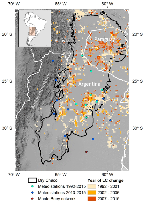
Figure 1Geographic location of the Dry Chaco ecoregion together with the spatiotemporal pattern of land cover (LC) changes obtained from the ESA-CCI land cover product (upscaled to 0.125∘ resolution) together with the location of the Monte Buey soil moisture site and in situ meteorological stations used for validation of soil moisture and precipitation, respectively.
2.2 Models
Three LSMs within the NASA LIS (Kumar et al., 2008) were selected to simulate land surface states and fluxes over the Dry Chaco: the Community Land Model version 2 (CLM2.0) (Bonan et al., 2002b; Oleson et al., 2004), Catchment LSM-Fortuna 2.5 (CLSM-F2.5) (Koster et al., 2000) and Noah LSM version 3.6 (Ek et al., 2003), hereafter simply referred to as CLM, CLSM and NOAH, respectively. More recent versions of these models are available and might provide better simulations over the Dry Chaco but are not yet implemented in the LIS. This study relied on the LIS to facilitate a consistent parameter revision across multiple LSMs, and one of the main goals was to see the impact of various LSM structures, regardless of their version. To demonstrate the impact of the updated soil treatment and dynamically evolving vegetation and land cover, a baseline simulation for each LSM was conducted and followed by various revised experimental runs. For all simulations, the spatial resolution was 0.125∘, and the output was created daily (model integration timestep of 15 min). The LSMs were spun up for 10 years from 1 January 1982 through 31 December 1991 using the land cover of 1992. The subsequent simulations from 1 January 1992 through 31 December 2015 were used for further analysis. The meteorological forcing data (precipitation, temperature, specific humidity, radiation, wind and surface pressure) were extracted from the Modern-Era Retrospective analysis for Research and Applications (MERRA-2) product (Gelaro et al., 2017) including gauge-based precipitation corrections (Reichle et al., 2017).
By default, the LIS LSMs use climatological LAI data based on a 4-year average derived from the Moderate Resolution Imaging Spectroradiometer (MODIS) Collection 4 LAI product (Kaufmann et al., 2000) and climatological global GVF data (Gutman and Ignatov, 1998) derived from 5 years of normalized difference vegetation index (NDVI) data from the Advanced Very-High-Resolution Radiometer (AVHRR) (Miller et al., 2006). The default land cover map is the University of Maryland (UMD) global land cover product (Hansen et al., 2000) based on AVHRR data from 1 April 1992 through 31 March 1993. The default soil properties in the LIS are derived from the FAO Soil Map of the World (FAO, 1971). In this study, vegetation, land cover and soil input data were revised using the Global Land Surface Satellite (GLASS) LAI (Liang et al., 2013; Xiao et al., 2016), the Global Inventory Modelling and Mapping Studies (GIMMS) NDVI (Tucker et al., 2005; Pinzon and Tucker, 2014), the ESA-CCI land cover product (Kirches et al., 2014; ESA, 2017) and soil properties derived from the HWSD v1.2 (FAO and ISRIC, 2012; De Lannoy et al., 2014).
2.3 Revised input data
2.3.1 GLASS LAI
The GLASS LAI product is a global spatiotemporally complete dataset, based on MODIS and AVHRR reflectance time-series data (Liang et al., 2013). This product is available for the period 1981–2015, with a temporal resolution of 8 d and a spatial resolution of 0.05∘ (Liang et al., 2013). Cloud-contaminated data are filled in using an optimum interpolation algorithm (Xiao et al., 2016). According to Liang et al. (2013) and Xiao et al. (2016), the GLASS LAI features more realistic and smoother seasonal variations than the MODIS LAI product (MOD15) (Knyazikhin et al., 1998) and the first version of the Geoland2 (GEOV1) LAI product (Baret et al., 2013). For the baseline simulations, a climatological LAI dataset was created using 24 years of GLASS data (1992–2015) to replace the default 4-year AVHRR climatology. This allowed us to solely display the effect of interannual and short-term vegetation variations in the revised experiments with time-varying GLASS data and land cover changes. The LAI observations were upscaled to the 0.125∘ resolution by spatial averaging.
2.3.2 GIMMS NDVI
The GIMMS NDVI product was assembled from AVHRR NDVI data (Tucker et al., 2005). The GIMMS dataset covers the period 1982–2015 and has a 15 d temporal resolution. The spatial resolution is 0.0833∘. The maps are 15 d maximum value composites, and cloud-contaminated pixels are replaced by NDVI values derived from either spline interpolation or average season profiles (Pinzon and Tucker, 2014). In this study, the GIMMS GVF was derived from its NDVI and used as input for the LSMs. According to Gutman and Ignatov (1998), the GVFi,j (–) is given by the following equation:
where NDVIi,j is the NDVI value observed at time i and pixel j and NDVImin and NDVImax are NDVI values over barren vegetation classes and fully covered vegetation classes, respectively. For simplicity, we chose to use the values proposed by Gutman and Ignatov (1998), i.e., 0.04 for NDVImin and 0.52 for NDVImax, and the GVF is restricted to the 0–1 interval. Multiple other approaches exist to derive GVF from NDVI, each with their own advantages and limitations (Jiang et al., 2010). For the baseline simulations, a climatological GVF dataset was created using 24 years of GIMMS GVF data (1992–2015). For the revised experiments with inclusion of land cover changes, the time-varying GIMMS data were used. To match the model's 0.125∘ resolution, NDVI values were upscaled by spatial averaging.
2.3.3 ESA-CCI land cover
The ESA-CCI land cover product offers yearly varying information on 37 land cover classes from 1992 through 2015 at a spatial resolution of 300 m (Kirches et al., 2014; ESA, 2017). This long-term land cover time series was achieved by combining surface reflectance data of different observation systems (Medium Resolution Imaging Spectrometer (MERIS), AVHRR, Satellite Pour l'Observation de la Terre (SPOT) Vegetation and PROBA-V) (Bontemps et al., 2012; Kirches et al., 2014). In this study, the ESA-CCI land cover maps were reclassified into 13 UMD classes (see Appendix A) and upscaled to a 0.125∘ resolution assigning the most dominant land cover to each pixel. Figure 1 shows how deforestation in the Dry Chaco has progressed in both time and space, based on this ESA-CCI land cover information. A static water mask file was created based on pixels that were classified as water at least once during the period 1992–2015. For CLSM, the UMD land cover classes were further combined into model-specific classes.
2.3.4 HWSD soil texture and SHPs
The global 1 km soil texture data were taken from the Soil and Terrain database for Latin America and the Caribbean as part of the HWSD v1.21 and were translated to 0.125∘ dominant soil texture. Similarly to in De Lannoy et al. (2014), the soil texture and organic matter data were used to estimate SHPs using the pedotransfer functions of Wösten et al. (1999). The derived SHPs include the soil porosity, bulk density, Clapp–Hornberger parameter B, saturated hydraulic conductivity, saturated matric potential, soil wilting point and field capacity (see Sect. 3.2.1). These HWSD-based soil parameters are also used in the operational Soil Moisture Active Passive (SMAP) Level-4 soil moisture product (Reichle et al., 2019).
2.4 Evaluation data
Precipitation input and surface soil moisture and evapotranspiration output were evaluated against in situ measurements and satellite-based estimates. Furthermore, an integrated evaluation of surface soil moisture, surface temperature and LAI was performed through the comparison of diagnosed L-band brightness temperature (Tb) simulations against satellite-observed Tb obtained from Soil Moisture and Ocean Salinity (SMOS).
2.4.1 Precipitation
The quality of the MERRA-2 precipitation over the Argentinean Chaco was evaluated against in situ data obtained from the Instituto Nacional de Tecnología Agropecuaria (INTA, 2020). Two sets of daily precipitation data were downloaded: data from meteorological stations covering the period 1992–2015 (10 stations) and data covering the period 2010–2015 (8 stations). The exact locations of these stations are shown in Fig. 1. As this study mainly focused on long-term simulations, the precipitation evaluation was conducted using monthly averaged data.
2.4.2 Monte Buey soil moisture
Pixel-scale in situ surface soil moisture was obtained from 17 nodes of the Monte Buey soil moisture network. The network is located in fields surrounding the town of Monte Buey, Cordoba, Argentina, just outside the Dry Chaco (Fig. 1), and covers three 0.125∘ model pixels. At each node, the surface soil moisture is measured using a Hydra Probe II buried at a depth of 5 cm. The network adopts the highest quality standards (Thibeault et al., 2015) and serves as a calibration and validation site for various satellite missions, e.g., the SAtélite de Observación COn Microondas and SMAP. To allow for comparison with the daily modeled surface soil moisture, averaged over three 0.125∘ model pixels, the hourly in situ measurements were averaged to daily values across the 17 nodes. The period of validation was from 1 January 2013 through 31 December 2015.
2.4.3 Evapotranspiration
The modeled evapotranspiration components were evaluated against Global Land Evaporation Amsterdam Model (GLEAM) data. The GLEAM consists of a set of algorithms that are driven by satellite-based observations and globally estimate all the daily evapotranspiration components at 0.25∘ spatial resolution (Miralles et al., 2011; Martens et al., 2017). Central in the GLEAM is the use of the modified Priestley and Taylor (1972) equation. Daily LIS simulations of latent heat flux were upscaled to 0.25∘ to allow for comparison to GLEAM data for the entire simulation period, i.e., 1992–2015.
2.4.4 L-band microwave brightness temperature
The satellite-observed L-band Tb data were extracted from the SMOS SCLF1C product, version 620, projected onto the 36 km Equal-Area Scalable Earth Grid, version 2 (EASEv2), angular fitted and quality controlled as in De Lannoy et al. (2015), e.g., excluding areas close to open water, urban areas, and areas with high radiofrequency interference or with a poor angular fit. Both the horizontally (H) and vertically (V) polarized data at a 40∘ incidence angle were used for evaluation of the daily simulations (see Sect. 3.5) from 1 January 2011 through 31 December 2015, using both ascending (06:00 LT) and descending (18:00 LT) half-orbits.
Table 1 summarizes the different experiments that were performed for each of the three selected LSMs. The experiments include a baseline (BL) simulation and two revised simulations, one with updated soil parameters (REVS) and one with both updated soil, vegetation and land cover parameters (REVSV) and two sensitivity simulations (SENSV, SENSLC), which are explained in Sect. 3.2.3.
3.1 Baseline simulations
The set of baseline (BL in Table 1) simulations used the default FAO surface soil texture data and the related default model-specific SHPs, assuming a vertically homogeneous soil profile for CLM and NOAH. By design, CLSM uses the 0–30 cm soil texture to compute parameters related to surface water transport, whereas the 0–100 cm soil texture is used for computation of all other parameters (Ducharne et al., 2000; De Lannoy et al., 2014). The vegetation input for the BL simulations consisted of monthly climatological vegetation datasets newly created based on GLASS LAI and GIMMS GVF, together with the ESA-CCI 1992 land cover map. This specific setup with climatological vegetation and static land cover does not account for major interannual changes in vegetation, e.g., due to deforestation. Note that CLM only requires LAI data, and GVF is not an input parameter.
3.2 Simulations with updated parameters
3.2.1 Revised soil parameters
In a first set of revised experiments, we replaced the model-specific SHPs (derived from FAO surface texture) for each LSM with the “topsoil” SHPs associated with a vertically homogeneous 0–100 cm HWSD soil texture and organic matter similar to in De Lannoy et al. (2014). Corresponding to the default structure of CLSM, only the 0–30 cm HWSD soil texture is used to obtain model-specific parameters for the surface soil water transport. In these experiments, only the soil parameters were revised (REVS in Table 1), whereas the climatological vegetation and land cover information was the same as in the BL simulations. Our hypothesis was that by feeding the different LSMs with similar SHPs, differences between model output could be reduced.
It is important to note that the different LSMs do not use the same subsets of SHPs. By default, CLM uses pedotransfer functions (Cosby et al., 1984) to relate sand and clay fractions to SHPs. The used SHPs in CLM are the saturated conductivity (Ksat), porosity (θsat), Clapp–Hornberger parameter B, and saturated matric potential (ψsat) (Han et al., 2014). The soil profile is divided into 10 layers, and Ksat decreases exponentially with depth throughout those layers.
CLSM's soil parameterization differs fundamentally from the other two LSMs. It uses several model parameters and moisture deficit model prognostic variables to dynamically partition the computational pixel into three distinctly different moisture regimes (saturated, transpiring and wilting regimes) to account for spatial variability of soil moisture within that pixel. CLSM's soil parameterization uses the spatial distribution of topographic indices and SHPs to derive model parameters (Ducharne et al., 2000). For baseflow generation only, CLSM assumes an exponential decay of Ksat with depth, with the decay factor ν=2.17 in the BL simulations and ν=1 in the REVS simulations, whereas for the vertical moisture transport, CLSM assumes Ksat to be vertically homogenous. Other important SHPs in CLSM are ψsat, the parameter B and soil wetness at wilting point θwilt.
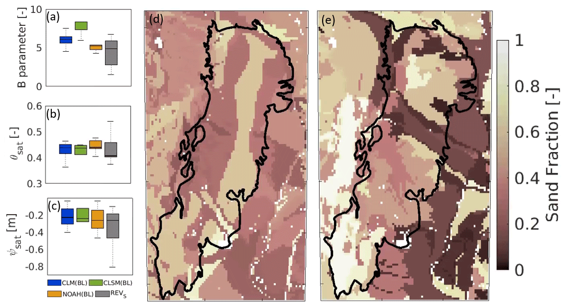
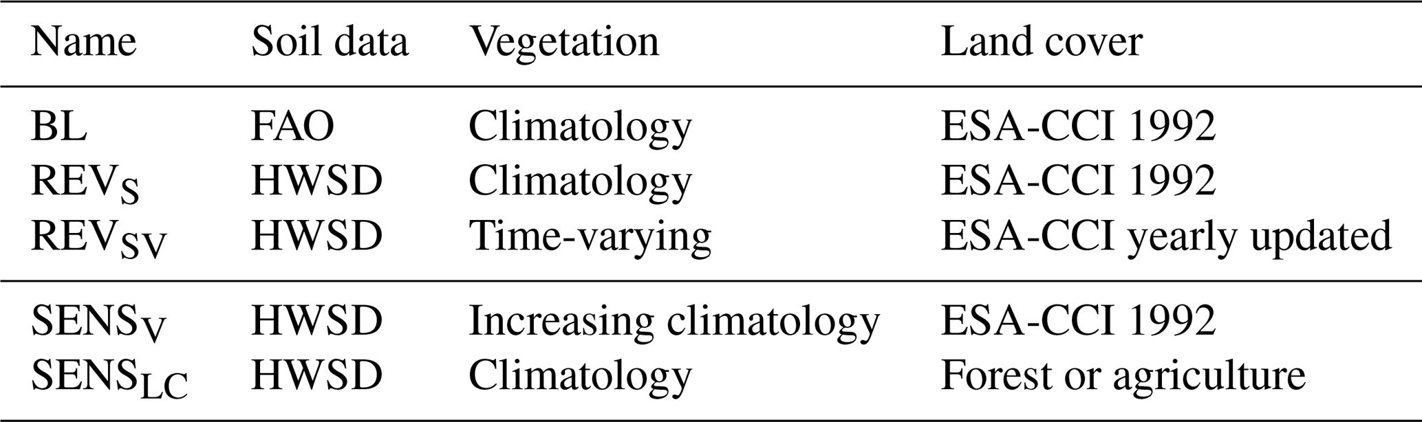
Figure 2Spatial boxplots of soil parameters: (a) B parameter, (b) porosity θsat and (c) saturated matric potential ψsat used in BL and REVS simulations. Sand fraction maps associated with (d) BL (FAO surface texture) and (e) REVS and REVSV (HWSD v1.21 0–100 cm texture).
The soil parameters in NOAH are discussed by Kishné et al. (2017), and the default SHPs are calculated from texture-based lookup tables (Cosby et al., 1984). The SHPs include the parameter B, θsat, ψsat, and Ksat. The soil profile is divided into four layers but with a constant Ksat value over depth (Ek et al., 2003). Other parameters include the soil water content threshold for ceasing evaporation from the top soil layer (DRYSMC), the saturated hydraulic diffusivity (SATDW), the soil water content at field capacity (REFSMC), soil wetness at wilting point θwilt, parameter for soil thermal diffusivity (F11) and quartz content (QTZ). Note that DRYSMC, SATDW, F11 and QTZ are not included in the SHPs of De Lannoy et al. (2014), and their values for the revised SHPs were derived from lookup tables based on the HWSD soil texture data.
The spatial boxplots in Fig. 2a–c show three SHPs used in the BL simulations of each LSM and their updated values used for the REVS and REVSV simulations over the Dry Chaco. The mean values for the updated B parameter, θsat and ψsat are smaller than for BL but have larger spatial variances. The slightly higher mean and standard deviation in the associated HWSD 0–100 cm sand fraction map (REVS: 43±25 %, Fig. 2e), compared to that of the FAO surface sand fraction map (BL: 41±15 %, Fig. 2d), explain the change in these updated parameter values.
3.2.2 Revised vegetation and land cover parameters
To analyze the response of the Chaco's hydrology to deforestation or vegetation changes in general, time-varying vegetation observations from GLASS and GIMMS were incorporated into the LSMs together with yearly updated ESA-CCI land cover maps in a second set of revised experiments (REVSV in Table 1). This specific setup includes the effect of vegetation changes (such as deforestation) compared to the use of climatological vegetation parameters and static land cover in the BL simulations. As described in Sect. 2.3.2 and 2.3.3, the GLASS LAI and GIMMS NDVI were available every 8 and 15 d, respectively. However, the data were linearly interpolated to obtain daily parameter updates in the LIS. The ESA-CCI land cover maps were updated each year on 1 January. LSMs only use land cover information to define model-specific parameters associated with each land cover type; i.e., ESA-CCI land cover is used as a predictor of parameters such as rooting depth, stomatal conductance and surface roughness. The exact values and implementation of each parameter are model-dependent.
Note that albedo calculations in each model were kept unchanged, as the focus of this study is primarily on the water balance. In CLM, the albedo for vegetated areas is calculated based on soil properties, LAI and plant functional types (Oleson et al., 2003). CLSM uses a surface albedo parameterization scheme (based on the Simple Biosphere Model, Sellers et al., 1986) that incorporates LAI, GVF and sun incidence angle to calculate the albedo and is rescaled to fit the annual cycle of MODIS-observed albedo. NOAH uses an albedo climatology based on 5 years (1985–1989) of visible and near-infrared radiation from AVHRR (Csiszar and Gutman, 1999). To see how deforestation influences the water budget component, the water budget analysis of the REVSV output mainly focused on the subset of 197 px that were deforested between 2002 and 2006 (based on the ESA-CCI land cover).
3.2.3 Sensitivity experiments
Our results will indicate (see Sect. 4.1.3) that the various LSMs react differently to the simultaneously updated interannually varying vegetation and land cover parameters. To disentangle the impact of vegetation and land cover parameters separately for each LSM, two sets of synthetic sensitivity experiments were conducted. A first set of sensitivity experiments (SENSV in Table 1) included five experiments (“exp1” through “exp5”) in which monthly spatially distributed climatological GLASS LAI values of the BL simulations were systematically increased by 1 and GVF values were raised proportionately. To estimate the corresponding GVF values, an empirical exponential relationship between LAI and GVF ())) was derived for each individual pixel based on daily LAI and GVF values from 1992 to 2000. LAI values much larger than about 6 do not occur in reality; nevertheless, they are kept in this sensitivity analysis to understand the LSM response in a synthetic setting. In CLM only the LAI was altered because CLM does not use GVF as an input, whereas both LAI and GVF were altered in CLSM and NOAH. Each experiment was run for the years 1992–2015 with a fixed ESA-CCI land cover map of 1992.
To test the sensitivity to land cover (SENSLC in Table 1), two simulations were conducted per LSM. In a first simulation, the entire Dry Chaco was assumed to be covered by deciduous broadleaf forest, whereas in the second scenario cropland was assumed. These vegetation classes are associated with the major land cover conversion in the Dry Chaco. The climatological GLASS LAI and GIMMS GVF datasets were used in SENSLC simulations.
3.3 Model evaluation in terms of water budget components
To assess the relative impact of different LSM structures, vegetation and land cover parameters, various water budget components were compared in each simulation:
where P is the precipitation (mm), ET is the total evapotranspiration (mm), Q is the total runoff (mm), and ΔS is the change in soil water storage (mm) for a given time period. The total ET and Q in the water budget equation (Eq. 2) can be written as the sum of their different components
where EV is the vegetation transpiration (mm), EB is the bare soil evaporation (mm), EI is the evaporation from canopy interception (mm), QS is the surface runoff (mm), and QSB is the subsurface runoff (mm).
3.4 Model evaluation with efficiency curves
The relative differences in the various LSM behaviors were further analyzed using efficiency curves, without associating any performance assessment. Q and ET are strongly regulated by soil moisture. However, soil moisture is also a highly model-dependent quantity (Koster et al., 2009), complicating the evaluation of the modeled Q and ET. To avoid this issue, Koster and Mahanama (2012) and Koster (2015) proposed to evaluate hydrological behavior in terms of “efficiency space”. The main reasoning behind this approach is that higher soil moisture content generally leads to both increased ET for a given amount of net incoming radiation (ET efficiency) and increased Q for a given amount of P (Q efficiency). The ET efficiency (–) is the ratio of the latent heat flux to the net radiation:
where λ (J kg−1) is the latent heat of vaporization, λET (J m−2) is the latent heat flux, Rnet (J m−2) is net incoming radiation and β(.) (–) is a function of moisture content, here assumed to be the 1 m soil moisture content mc1 m. The Q efficiency (–) is the ratio of the total Q production to the total P:
where Q is total runoff, P is the precipitation and F(.) (–) again is a function of mc1 m. By plotting the Q efficiency against ET efficiency and identifying their relationship, a unique signature of the hydrological behavior (without model-dependent soil moisture) of a LSM can be obtained. Ideally, this would allow us to shift a LSM signature towards an in situ observed land surface signature. Due to lack of suitable and publicly available Q measurements for the Dry Chaco, this study uses the efficiency space to relatively compare the hydrological behavior of different LSMs with various parameter settings (BL, REVS, REVSV).
For each pixel, water budget components (λET, Rnet, Q, mc1 m and P) were averaged over each month for the period 1992–2015. Different locations had different minimum mc1 m values, induced by differences in soil texture. Prior to plotting, the mc1 m values for each pixel were normalized to reduce spatial differences in mc1 m and to dominantly focus on the temporal LSM signature. Both the Q and ET efficiency were plotted as a function of the normalized mc1 m for each LSM to visualize the model-specific soil moisture dependencies. For each pixel, a curve drawn through the points was constructed by computing the median of the ET and Q efficiencies over narrow bins of normalized mc1 m. The combination of all fitted curves for all pixels was visualized using a scatter density cloud. The resulting “efficiency space” plots (showing the obtained ET efficiency as a function of Q efficiency) show how evaporation and runoff efficiencies vary with each other as the soil gets drier or wetter. The efficiency plots are used to see whether the three LSMs provide a consensus on the simulated hydrological behavior and on the impact of the updated soil, vegetation and land cover treatment.
3.5 Model evaluation with independent data
For each experiment, the quality of model input P and the model performance in terms of output surface soil moisture content (sfmc) and ET were evaluated against independent data (Sect. 2.4), for simplicity referred to as “observations”, using four skill metrics:
-
bias: long-term mean difference between simulations and observations (i.e., model minus observation),
-
ubRMSD: unbiased root‐mean‐square difference, calculated by first removing the bias from both the simulated and observed time series (Entekhabi et al., 2010),
-
R: temporal Pearson correlation coefficient between simulations and observations,
-
aR: temporal anomaly Pearson correlation coefficient between simulations and observations, calculated after removing the mean climatology from each time series. The climatology is computed as the multi-year average of 30 d smoothed time series of daily values. This removed the trivial agreement in seasonality and allowed us to focus on interannual and short-term dynamics.
For an integrated evaluation of the model sfmc, surface temperature and LAI of the various experiments, a zero-order tau-omega microwave radiative transfer model (RTM) was used to convert these modeled variables into L-band Tb (K) estimates. The modeled Tb were compared to SMOS Tb observations, similarly to the approach presented by Albergel et al. (2012). For a detailed description of the tau-omega RTM, we refer to De Lannoy et al. (2013). Feldman et al. (2018) showed that a zero-order tau-omega model would suffice for the dry forests of the Dry Chaco. Instantaneous sfmc, surface temperature and LAI at 06:00 and 18:00 LT were used as input in the RTM, and simulated Tb were evaluated against 06:00 and 18:00 LT SMOS-observed Tb (both at the top of vegetation). The Tb simulations were computed at the 0.125∘ model resolution and then spatially averaged to the 36 km EASEv2 grid for comparison to SMOS-observed Tb for the period 2011–2015. Short-term variability in both simulations and observations was reduced using a 1-month averaging window. This allowed us to focus on the effect of the implemented vegetation changes, which occur on a longer seasonal timescale.
The RTM required specific input parameters related to soil properties (Wang and Schmugge, 1980) and vegetation classes. The related soil parameters differ thus for the BL and REVS simulations, and the parameters related to land cover class also vary in time for the REVSV simulations due to yearly updated land cover. The literature offers various lookup tables to estimate the RTM parameters related to vegetation classes (soil roughness, scattering albedo, vegetation structure parameters). Here, we used the lookup tables of the SMAP soil moisture retrieval (O'Neill et al., 2015; Quets et al., 2019). Another choice would affect the overall Tb bias for all experiments but would minimally affect the relative comparison of the various experiments with revised soil and vegetation parameters.
4.1 Model evaluation in terms of water budget components
4.1.1 Baseline simulations
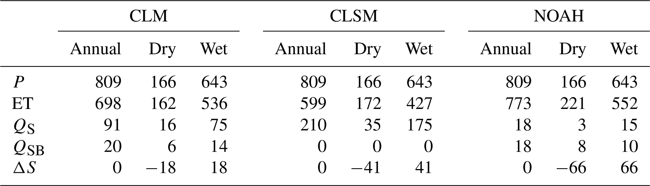
The annual and seasonal distributions of the different water budget components for each BL model simulation are summarized in Table 2. The values are calculated for a 24-year period (1992–2015) and averaged over all pixels within the Dry Chaco, excluding open-water pixels. The Dry Chaco receives an average yearly P of 809 mm, with most P (643 mm) during the wet season (October–March), in line with the findings of Marchesini et al. (2020) and Minetti et al. (1999). All LSMs confirm a water storage (ΔS) deficit for the dry season (April–September), which is compensated for during the wetter months with a water surplus. Figure 3a shows the corresponding yearly averaged water budget components relative to the total P whereby the total ET is subdivided into its three components (see Sect. 3.3). The variation in the total amount of ET and its components shows that there is large variability between the models, even though all of them use the same forcing data, land cover, vegetation, soil texture (not SHP) and topography input. In addition, there are significant disagreements in the ET partitioning. The largest ET component is different in each LSM; i.e., EI is largest for CLM, EB for CLSM and EV for NOAH. The high fraction of EI for CLM is physically unrealistic (see Sect. 5). CLM and NOAH both have a QSB component, whereas CLSM does not. The latter has a very large fraction of QS.
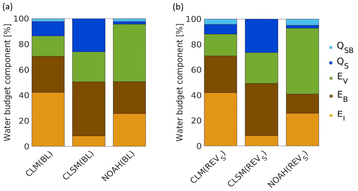
Figure 3Long-term (1992–2015) annual water budget components averaged over the Dry Chaco relative to the total precipitation for the (a) BL and (b) REVS experiments (QSB: subsurface runoff, QS: surface runoff, EV: vegetation transpiration, EB: bare soil evaporation, EI: interception evaporation).
Table 2Long-term (1992–2015) distribution of the BL water budget components (mm) for CLM, CLSM and NOAH over the Dry Chaco, year-round (annual), for the months April–September (dry season) and the months October–March (wet season), respectively.
4.1.2 Revised soil parameters
The impact of the revised soil parameters (REVS) on the yearly mean relative water budget components is shown in Fig. 3b, again for the period 1992–2015. Most striking is that, despite the similarity in SHPs, the various models still produce a very different partitioning of the water budget components. For CLM, the revised SHPs cause a yearly reduction in QS by 4 % which is compensated for by an increase in EV and QSB. For CLSM, the mean water budget components hardly change. For NOAH, there is a small increase in QSB and a decrease in ET, mainly due to a large decrease in EB (−9 %), of which 6 % is compensated for by extra EV. For each model, the differences in the water budget components between the BL and REVS simulations, averaged over the entire Dry Chaco, are relatively small. However, within the study domain, there is a large local spatial variability in the changes in the various water budget components (not shown).
Figure 4 summarizes the impact of the updated SHPs on the soil moisture content in the first meter of the soil (mc1 m). The boxplots of time-averaged (1992–2015) mc1 m over the Dry Chaco (Fig. 4a) show that the REVS simulations are drier than for BL: the mc1 m decreases from 0.16 to 0.11 m3 m−3 for CLM, from 0.22 to 0.13 m3 m−3 for CLSM and from 0.19 to 0.17 m3 m−3 for NOAH. These lower mean soil moisture values can be related to the larger fraction of sandy soils (Fig. 2d and e) and the associated reduced water retention (SHPs) in the REVS simulations. However, again, at the local scale, some areas become wetter and others drier. Despite the relatively large difference in long-term mean soil moisture between BL and REVS, the differences in ET and QS fluxes are small: the meteorological forcings are the primary drivers of these fluxes, whereas the SHPs only have a secondary impact. Figure 4c and d show how the texture pattern dominates the long-term averaged mc1 m for the period 1992–2015 for the NOAH BL and REVS simulations (similarly for CLM and CLSM). Figure 4b illustrates that the updated SHPs change the temporal standard deviation of mc1 m, which significantly decreased for NOAH.
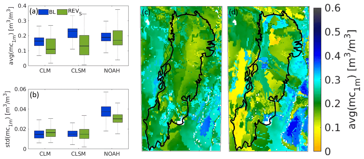
Figure 4Boxplots of long-term (1992–2015) (a) average (avg) and (b) standard deviation (SD) of BL and REVS moisture content in the upper 1 m (mc1 m) for CLM, CLSM and NOAH. Maps of long-term (1992–2015) average NOAH mc1 m, obtained with (c) BL and (d) REVS parameters.
4.1.3 Revised vegetation and land cover parameters
The impact of deforestation over the Dry Chaco was assessed via a relative comparison of the water budget components of the REVS and REVSV simulations for each LSM, using a subset of 197 px that was deforested between 2002 and 2006. Keep in mind that the REVS uses climatological vegetation indices and a static land cover map, which do not account for interannual vegetation changes. The REVSV simulations include the effects of vegetation changes by the implementation of satellite-derived dynamic vegetation indices as well as yearly updated land cover parameters. The differences between the REVS and REVSV simulations thus solely stem from interannual vegetation variations and land cover changes. By design, the former would only introduce minimal long-term differences over the entire simulation period. Therefore, the output differences were only analyzed after deforestation, i.e., for the period 2007–2015. Figure 5 compares the water budget components for the REVS and REVSV simulations after deforestation, i.e., for the period 2007–2015. For CLM, we observed a relative decrease in EV (−6 %) that is compensated for by an increase in EB and EI, maintaining a constant amount of ET. For CLSM, there is a 5 % decrease in total ET (with a similar relative distribution of the ET components), which is compensated for by a QS increase of 5 %. For NOAH, deforestation also resulted in smaller ET (−3 %), which is compensated for by an increase in QSB. Regarding the relative ET distribution of NOAH, there is an increase in EB of 4 % and a decrease in EV of 6 %.

Figure 5Annual water budget components for the period 2007–2015 relative to the total precipitation for the 197 px deforested between 2002 and 2006 for REVS and REVSV simulations (QSB: subsurface runoff, QS: surface runoff, EV: vegetation transpiration, EB: bare soil evaporation, EI: interception evaporation).
The impact of vegetation changes on the temporal evolution of LAI and moisture content in the first 2 m of the soil (mc2 m) is illustrated in Fig. 6 for a representative pixel (28.0625∘ S, 63.6875∘ W). Figure 6a shows the climatological REVS LAI and the interannually varying REVSV LAI, together with P for a pixel that was deforested in 2004 (based on ESA-CCI land cover). The LAI values are generally low both before and after deforestation. Years where the REVSV LAI is larger than its climatology mainly correspond to wetter years. Deforestation does not cause a sudden drop in LAI, probably because the LAI for fully developed crops is not very different from that of dry forests, or the smaller-scale deforestation signal may be suppressed in the upscaled 0.125∘ LAI values. However, the REVSV LAI is significantly smaller than its climatology in drier years after 2004, which may be indicative of less crop cover and earlier deforestation. In short, the coarse-resolution LAI does not necessarily reflect land cover changes and is strongly influenced by P.
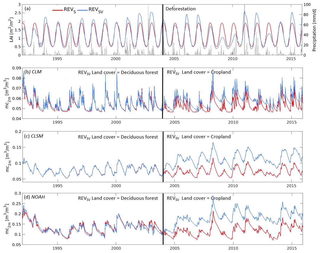
Figure 6Time series of REVS and REVSV land surface variables for a pixel deforested in 2004 (28.0625∘ S, 63.6875∘ W): (a) LAI and precipitation; (b, c, d) 2 m moisture content (mc2 m) for CLM, CLSM and NOAH, respectively.
The combined impact of time-varying LAI and land cover on mc2 m is shown in Fig. 6b–d for the REVS and REVSV simulations of each LSM. From the deforestation in 2004 onwards, the mc2 m of the REVSV simulations increases for each model, but at a different rate. The main driver for the increase in mc2 m is the change in land cover. The updated parameters related to a land cover change push the model out of its equilibrium, and water is gradually redistributed to achieve a new balance with a higher soil moisture content. Considering all pixels deforested between 2002 and 2006, mc2 m increases on average by 0.0035 m3 m−3 (maximum change of 0.016 m3 m−3) for CLM, by 0.03 m3 m−3 (maximum change of 0.08 m m3 m−3) for CLSM and by 0.07 m3 m−3 (maximum change of 0.1 m3 m−3) for NOAH. The reason for the different behavior of each LSM will be explained in the following paragraph.
4.1.4 Sensitivity experiments
Sensitivity experiments with synthetic vegetation and land cover parameters were conducted to get more insight into the distinct behavior of soil moisture for the different LSMs in response to dynamic vegetation and land cover input. Figure 7a–c illustrate how domain-averaged water budget components change when the LAI is systematically increased by 1 to 5 units (“exp1” through “exp5”) as explained in Sect. 3.2.3. To mimic the effect of deforestation, assumed to result in smaller LAI values, one should read the figure from exp5 (high LAI) to exp1 (low LAI). For CLM, a reduction in LAI introduces a reduction in EI, an increase in EB and a slight decrease in EV. For CLSM, a reduction in LAI and GVF yields a strong decrease in EI, fully compensated for by an increase in EB, whereas EV is barely affected. Concerning NOAH, smaller LAI and GVF values result in a significant decrease in EV. When the LAI and/or GVF are reduced, the QSB increases in both CLM and NOAH.
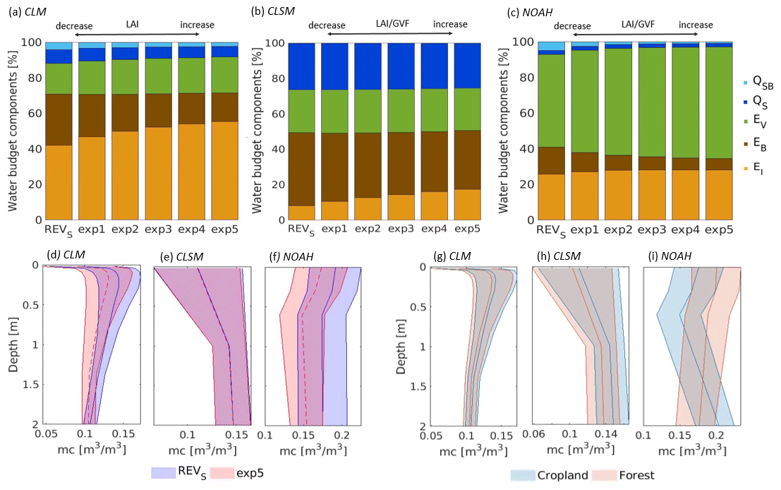
Figure 7(a–c) Long-term (1992–2015) water budget components averaged over the Dry Chaco for SENSV experiments, for CLM, CLSM and NOAH, respectively. Exp1 to exp5 refer to simulations whereby the monthly climatological LAI maps were increased by, respectively, 1 to 5 units (QSB: subsurface runoff, QS: surface runoff, EV: vegetation transpiration, EB: bare soil evaporation, EI: interception evaporation). (d–f) Associated impact on the soil moisture profile (spatially averaged profile) for CLM, CLSM and NOAH, respectively. (g–i) Impact of changing land cover parameters (SENSLC) from deciduous forest to cropland on the soil moisture profile for CLM, CLSM and NOAH, respectively.
Figure 7d–f illustrate how the various LSM soil moisture profiles respond to changing LAI (and corresponding GVF for CLSM and NOAH). A decrease in LAI barely affects soil moisture in CLSM, whereas it increases soil moisture for CLM (moderately) and NOAH (strongly), in line with the respective LSM's degree of decrease in EV (water extraction from the soil). The increase in soil moisture climatology for an imposed decrease in LAI (while assuming a persistent vegetation type) is partly an artifact resulting from a one-way dependency of soil moisture to vegetation in the absence of a dynamic vegetation growth module. In nature, LAI and soil moisture evolve together.
Figure 7g–i show soil moisture profiles for the sensitivity experiment in which the land cover was either uniformly cropland or forest. For CLM, there is almost no difference in soil moisture between both. CLSM has a slightly wetter soil moisture profile for cropland than for forest. For NOAH, the soil moisture content is higher under cropland than forest in the deeper layers. The distinct model response to land cover changes is related to the fact that each model uses a model-specific set of land cover parameters, each with different values and behavior. These parameters impact the total EV (not shown) and the related water extraction from the soil. For example, the rooting depth (the depth to which roots of plants can extract water from the soil profile) is defined differently in each LSM. In NOAH, the forest land cover class has a rooting depth of 2 m; i.e., roots take up water over the whole profile. Roots of crop are parameterized to 1 m and are not able to extract water from the deepest soil layers, resulting in wetter soils at the bottom of the soil profile (Fig. 7i). CLM makes use of a root fraction distribution whereby root fraction is a function of depth and land cover type as described in Zeng (2001). CLSM uses a rooting depth of 1 m, regardless of the land cover.
The sensitivity experiments were designed to explain the distinct behavior of soil moisture in response to changing land cover or vegetation parameters separately and do not provide insights into possible interactions between both. The relative change in the water budget components of REVSV against REVS, as shown in Fig. 5, originates from changes in LAI and GVF, land cover, and their interactions. This explains, for example, the increase in model QS and decrease in total ET after deforestation for CLSM. This cannot be explained by the CLSM results of the SENSV (Fig. 7b) or SENSLC experiments alone.
4.2 Model evaluation with efficiency curves
4.2.1 Baseline simulations
To compare the BL hydrological behavior of the three different LSMs, Fig. 8 presents the Q and ET efficiency as a function of mc1 m along with the “efficiency space”. For each pixel within the Dry Chaco, these quantities are computed for each month across the 24-year time period, and a curve is fitted using a simple binning procedure. Figure 8 summarizes the hydrological signature of the Chaco by showing the density scatter cloud of all fitted curves.
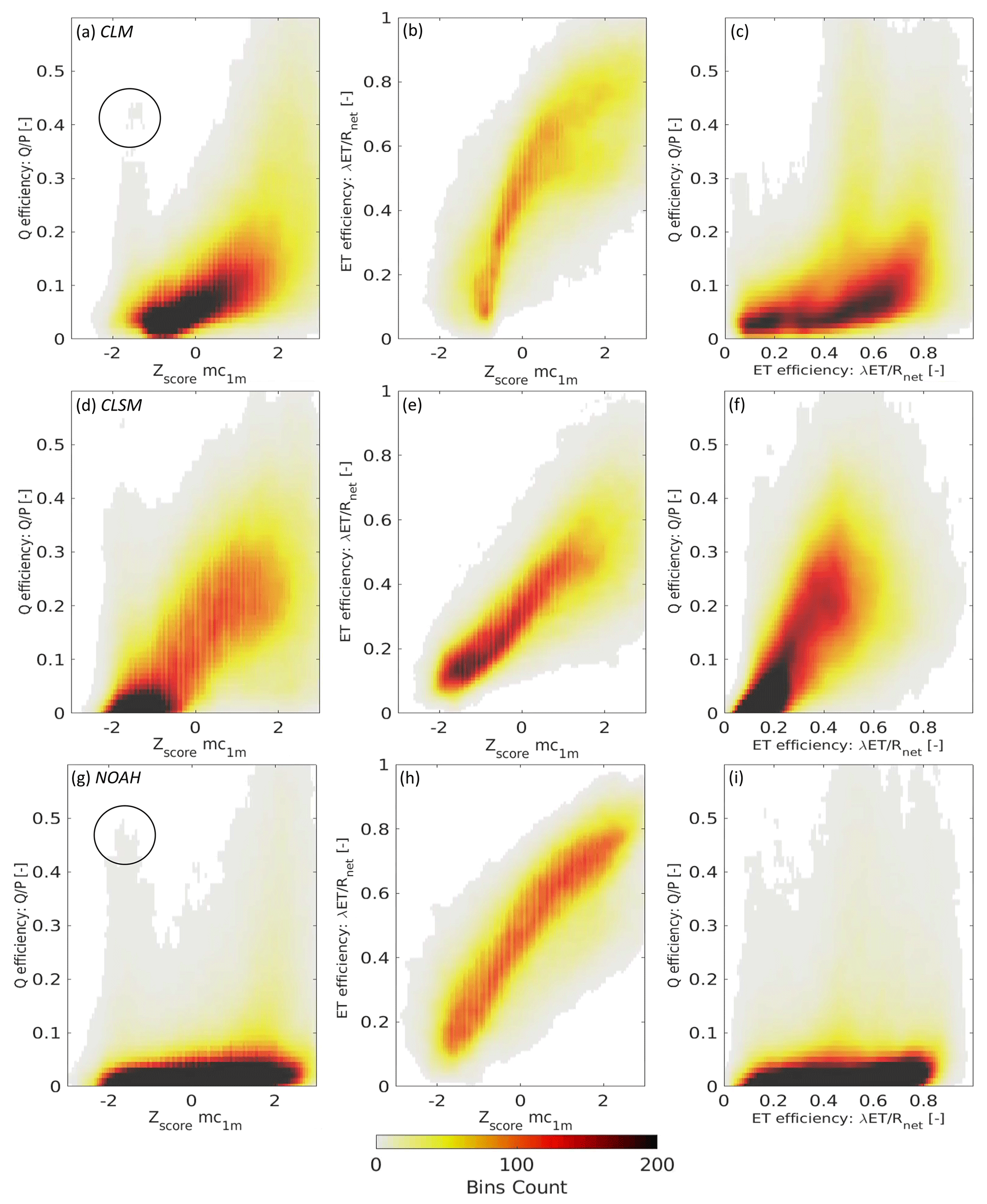
Figure 8Scatter density clouds representing the fitted curves in efficiency space of all pixels inside the Dry Chaco for the BL experiment for the period 1992–2015 for (a–c CLM, (d–f) CLSM and (g–i) NOAH, respectively. (a, d, g) Q efficiency, (b, e, h) ET efficiency and (c, f, i) ET vs. Q efficiency.
Figure 8a, d and g show a very different Q efficiency as a function of mc1 m for the three LSMs. For CLSM, a majority of the curves reaches Q efficiency values up to 0.4, whereas the median values are around 0.2 for CLM and even below 0.1 for NOAH. This different behavior was also observed in the annual water budget analysis (see Table 2). Note that for CLM and NOAH, some high Q efficiencies are found at relatively low mc1 m values (black circle). This is caused by high QSB rates, which allow precipitation from the wet season to run off during the dry season months even if P in the latter period is small.
For all LSMs, the ET efficiency (Fig. 8b, e and h) is larger than the Q efficiency, and the relationship of the ET efficiency with mc1 m is more similar across the three LSMs than that of the Q efficiency. The distinct BL signature of the three LSMs in efficiency space is summarized in Fig. 8c, f, i and mainly explained by differences in Q.
4.2.2 Revised simulations
Figure 9 shows the impact of the REVS and REVSV experiments in efficiency space. The impact of the updated SHPs is summarized by a small shift between the mean values of the BL and REVS in efficiency space, with a decrease in Q efficiency for CLM and increase for CLSM and NOAH.
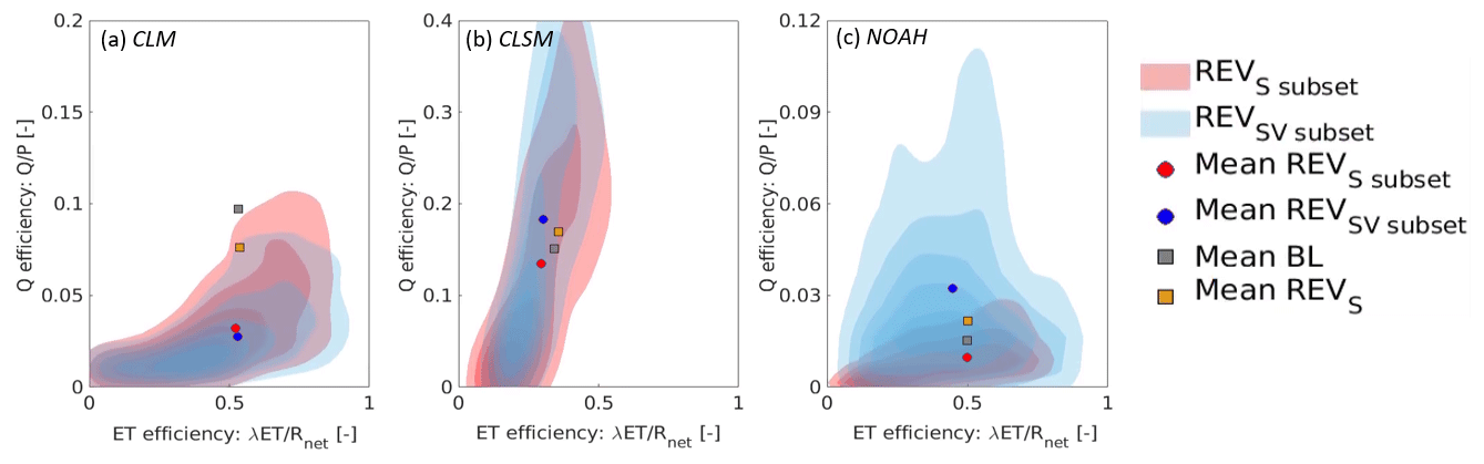
Figure 9Scatter clouds in efficiency space for the REVS (red) and REVSV (blue) experiment for a subset of 197 px (corresponding to deforested pixels between 2002 and 2006) for the period 2007–2015, together with the mean value for (a–c) CLM, CLSM and NOAH, respectively. The gray and orange dots represent the shift in mean efficiency between the BL and REVS simulations, based on all pixels inside the Dry Chaco; i.e., the mean BL values correspond to those in Fig. 8c, f and i.
Figure 9 also shows the REVS and REVSV scatter density clouds (and mean value) in efficiency space for the 197 px deforested between 2002 and 2006 for the period 2007–2015. The inclusion of vegetation changes (REVSV) causes a shift towards larger Q efficiencies for CLSM (increased QS) and NOAH (increased QSB). The opposite is found for CLM. When analyzing the effect of deforestation on ET efficiency, it is important to keep in mind that these efficiencies are calculated as the ratio of the latent heat flux to the net incoming radiation (available energy). By definition, the net radiation is also impacted by vegetation changes. Therefore, one cannot directly relate changes in ET efficiency to changes in total ET. For CLM, the REVSV density cloud tends to larger ET efficiencies, indicating that croplands need less energy than forests for the same amount of ET. For CLSM and NOAH, the scatter cloud shows a slight shift to the right: croplands use a slightly larger portion of the available energy than forest for ET.
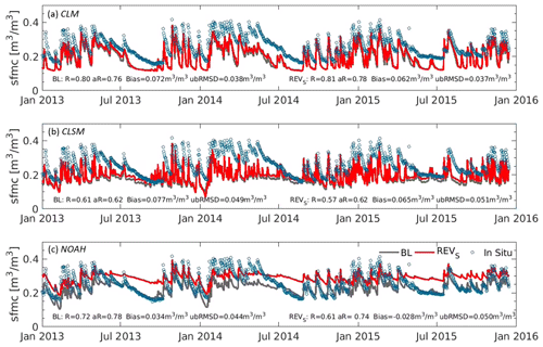
Figure 10Simulated (BL and REVS) and in situ observed surface soil moisture (sfmc) time series at Monte Buey, Argentina (32.91∘ S, 62.44∘ W), for the period January 2013–December 2015, for (a–c) CLM, CLSM and NOAH, respectively.
4.3 Model evaluation with independent data
4.3.1 Precipitation
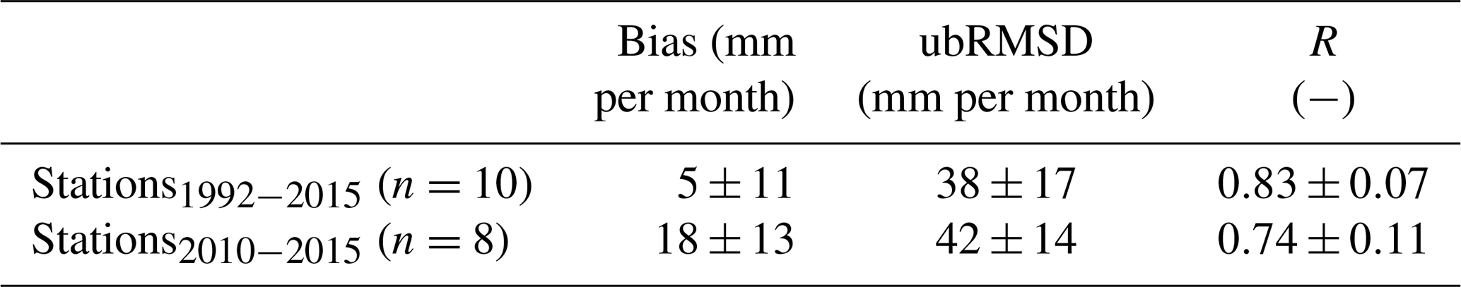
Because the quality of input P will greatly influence the quality of ET, sfmc and Tb simulations, independently of the used LSM, the quality of the MERRA-2 P product was first evaluated against in situ P data. Table 3 summarizes how well the monthly averaged MERRA-2 P corresponds to in situ observations for two types of stations. For the 10 stations that cover the 1992–2015 period, the mean correlation coefficient is 0.83 (±0.07), the mean monthly bias is 5 (±11) mm per month and the mean ubRMSD equals 38 (±17) mm per month. For the 2010–2015 stations (n=8), the overall skill metrics are lower: a mean correlation of 0.74 (±0.11), a mean bias of 18(±13) mm per month and a mean ubRMSD of 42 (±14) mm per month, respectively. The positive bias indicates that MERRA-2 P is overestimated.
Table 3Skill metrics for monthly MERRA-2 relative to in situ precipitation: spatial average ± spatial standard deviation.
4.3.2 Monte Buey soil moisture
Figure 10 shows daily modeled sfmc time series for CLM, CLSM and NOAH, together with in situ Monte Buey sfmc (5 cm) observations (both averaged over 3 px) for the period 2013–2015. For CLSM and NOAH, the sfmc depths are 2 and 10 cm, respectively. For CLM, the soil moisture content in the four upper soil layers was averaged to obtain a 5 cm sfmc value.
The largest R and aR values between observed and modeled sfmc are obtained with CLM and NOAH (R and aR values between 0.72 and 0.81 for BL). By updating the soil parameters (REVS), some R and aR values increase, but others decrease. However, the bias is decreased for all models. For NOAH, the updated soil parameters result in substantially wetter sfmc during the dry season. Note that these results are only valid for the 3 model pixels covering the Monte Buey site and cannot be extended to the entire Dry Chaco.
4.3.3 Evapotranspiration
The skill of daily simulated total ET relative to that of GLEAM-based ET estimates is shown in Fig. 11a–d for the period 1992–2015 over the entire Dry Chaco. In general, NOAH has the largest R and aR and the smallest ubRMSD. When averaged across the entire region and time period, the impact of the updated soil, vegetation and land cover parameters on the total ET is negligible and even deteriorates the overall CLSM performance relative to GLEAM.
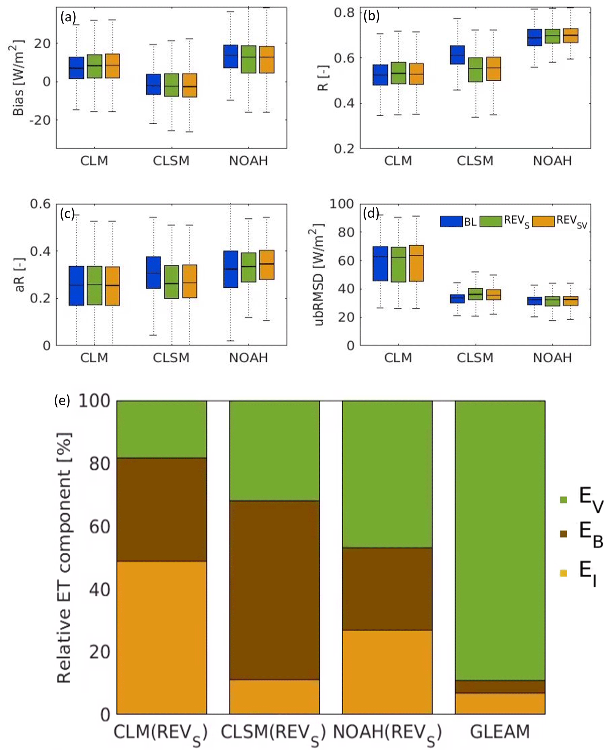
Figure 11(a–d) Skill metrics for total ET from CLM, CLSM, and NOAH (BL, REVSV and REVSV) relative to GLEAM, calculated for the period 1992–2015 over all pixels inside the Dry Chaco. (e) Long-term (1992–2015) relative ET components (EV: vegetation transpiration, EB: bare soil evaporation, EI: interception evaporation) spatially averaged over the Dry Chaco for REVS CLM, CLSM, NOAH and GLEAM.
The relative distribution of the different ET components is very different for GLEAM than for the selected LSMs. Figure 11e shows that all the models (REVS) are possibly underestimating the EV. For GLEAM, 89 % of the total ET is EV, whereas this is only 47 % for NOAH, 31 % for CLSM and 18 % for CLM. EI is the second largest component in GLEAM (7 %). CLM (48 %) and NOAH (27 %) are likely overestimating the EI, whereas CLSM overestimates the EB.
4.3.4 L-band microwave brightness temperature
Time series of the simulated 40∘ Tb at horizontal polarization () with NOAH BL, REVS and REVSV input and SMOS are shown in Fig. 12a. The inputs used in the RTM for the simulated Tb include simulated surface soil moisture (using FAO texture and related SHPs in the BL simulations and HWSD-based texture and SHPs in the REVS and REVSV simulations), temperature, LAI (climatological in BL and REVS, interannually varying in REVSV), land cover (static in BL and REVS, yearly updated in REVSV) and the associated literature-based lookup RTM parameters. These time series are for the 36 km EASEv2 pixel that includes the deforested 0.125∘ pixel shown in Fig. 6. The corresponding sfmc and LAI are shown in Fig. 12b and c. Time series of NOAH Tb at vertical polarization () and the simulations for CLM and CLSM showed similar behavior and are not shown. Figure 12 highlights how the REVSV LAI deviates from the long-term climatology (REVS) during the SMOS observation period. Not shown here is that the LAI also deviates from the climatology earlier in time; i.e., on average the interannual variations cancel each other out by design, as in Fig. 6.
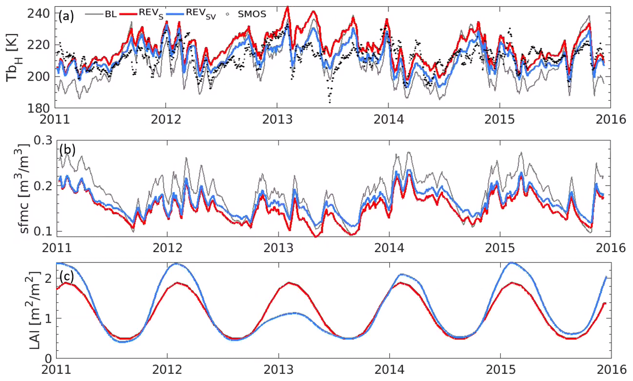
Figure 12Time series of simulated (gray) BL, (red) REVS, and (blue) REVSV NOAH-based (a) , (b) sfmc and (c) LAI input at the same location as in Fig. 6 but upscaled to the 36 km EASEv2-grid resolution. Also shown are (black dots) SMOS observed in subplot (a).
The updated soil parameters (REVS) affect the sfmc and RTM parameters, causing a different behavior in simulated . The reduced LAI and changes in land cover (REVSV) result in wetter sfmc, but the sfmc increase is not as pronounced as for the mc2 m in Fig. 6d. This wetter sfmc and reduced LAI propagate through the RTM and result in colder simulated .
Figure 13a–d summarize the Tb skill metrics for the different experiments, only for the subset of pixels that were deforested between 2002 and 2006. The metrics for both polarizations ( and ) were averaged before creating the spatial boxplots. In general, the Tb bias for each model is negative, indicating that the simulated Tb is colder than the SMOS Tb. NOAH has the largest absolute bias, and the updated soil treatment reduces the Tb bias of each model. CLSM has the best R and aR values, but the updated soil parameters reduce its performance in terms of R, aR and ubRMSD values. This is in line with the reduced performance of CLSM relative to the GLEAM ET. For NOAH, the updated soil treatment increases the R and aR values and reduces the ubRMSD. The additional impact of the updated vegetation and land cover treatment is small.
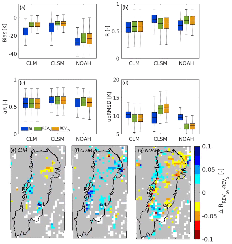
Figure 13(a–d) Skill metrics for CLM, CLSM, and NOAH (BL, REVSV and REVSV) Tb relative to SMOS Tb, calculated for the period 2011–2015 over pixels deforested between 2002 and 2006. (e–g) Difference between the R metric for REVSV and REVS for CLM, CLSM and NOAH, respectively.
To visualize the local effects of the vegetation changes, spatial maps of the differences in temporal R values (ΔR) between the REVSV and REVS are shown for each model in Fig. 13e–g. The modeled Tb and the spatial pattern of ΔR over the Dry Chaco are mainly driven by changes in sfmc, and these are driven by vegetation and land cover changes. The ΔR values are relatively small for CLM because the model sfmc is only slightly sensitive to changes in vegetation and land cover parameters. For CLSM, the REVSV simulations yield larger R values over certain areas compared to the REVS simulations because temporal changes in modeled sfmc mainly result from changes in land cover parameters. Consequently, the ΔR pattern is similar to the deforestation pattern (see Fig. 1). In NOAH, the sfmc is sensitive to land cover and LAI changes and, therefore, the ΔR pattern depends on both land cover and LAI changes. For NOAH, the ΔR values do not increase everywhere. At some pixels with reduced REVSV performance, we noticed unexpected trends in the LAI time series (not shown); i.e., LAI would not show the expected decrease during the dry season. This possibly deteriorated the Tb simulations. In short, the extent of the simulated Tb response to vegetation and land cover changes is model-specific and is mainly driven by the sensitivity of the model's sfmc to vegetation and land cover parameters.
5.1 LSM comparison
The relative evaluation of LIS CLM, CLSM and NOAH in terms of their water budget components (Table 2 and Fig. 3) and efficiency space (Fig. 8) highlights that each LSM has a distinct hydrological signature. CLSM has more QS than NOAH and CLM, but CLSM has no QSB component, unlike NOAH and CLM. It is striking how the various LSMs partition the total ET very differently into its three components, as was reported before by Wang and Dickinson (2012), Kumar et al. (2018), Rigden et al. (2018) and Zhang et al. (2020). For example, we found that CLM strongly overestimates EI and EB compared to GLEAM over the Dry Chaco (Fig. 11e). Lawrence et al. (2007) came to similar findings and indicated that by reducing the tuning parameter αl from 1 to 0.25 in the canopy interception equation, the amount of EI could be reduced to more realistic values at the global scale. They also indicated that the relative contribution of EV and EB in vegetated regions could be improved by altering two parameters (Cs,dense and α) in the equation to calculate the turbulent transfer coefficient between the soil and canopy air. For CLSM, the portion of EI over the Dry Chaco is similar to that of the GLEAM product. Reichle et al. (2011) described how the amount of interception evaporation is influenced by the rainfall interception parameters FWETL and FWETC and that realistic interception rates are found when both parameters equal 0.02 (applied in our simulations). These parameters describe the fractional areas of canopy leaves (interception reservoir) on which large-scale and convective rainfall is applied. The bias between modeled ET and GLEAM is high for NOAH, indicating an overestimation of the total ET. Wei et al. (2013) observed that NOAH yields substantial biases in latent heat flux, total Q and land surface skin temperature when compared to independent data over the United States. They showed that adapting model parameterizations, such as including a seasonal factor for the root distribution and selecting optimal model parameters related to the canopy resistance calculations (an important factor for EV simulation), could reduce these biases.
Our results show that constraining the LSMs with the same optimal soil, vegetation and land cover parameter input (REVS and REVSV) does not result in more similar water budget partitioning, because the results are dominated by internal model-specific equations and parameters. The latter have historically been tuned globally with particular input datasets and may compensate for errors in those datasets, so that “better” input does not necessarily lead to “better” output. In addition, some LSMs are inherently more or less sensitive to time-varying parameters, and therefore climatological vegetation input may suffice if the LSM is simply not very sensitive to vegetation changes (Jarlan et al., 2008) or if the vegetation changes are not extensive. LSMs could benefit from further development to obtain a more realistic hydrologic response to vegetation changes and to better include dynamic vegetation phenology. This should lead to more realistic simulations of the interaction between the carbon and water cycles.
Lack of sufficient in situ Q and ET measurements over the Dry Chaco prevents identification of which LSM setup best approaches the long-term observed water budget and its components. However, our study highlights the large estimation uncertainty due to model structures and the secondary impact of (soil and vegetation) input parameter uncertainties. It is important to mention again that LSMs are continuously upgrading and that our study provides a relative comparison of older LSM versions within the LIS.
5.2 Effects of soil and vegetation parameters on soil moisture
Despite soil moisture being a highly model-dependent variable, it is important that soil moisture simulations closely mimic natural patterns to allow their use as underlying information in applications such as soil salinity monitoring over the Dry Chaco. Providing LSMs with the best available soil and vegetation parameters is one step towards this goal. The soil parameters strongly determine the spatial (horizontal and vertical) pattern of soil moisture (Fig. 4) and only have a secondary impact on its temporal variability, which is mainly driven by meteorology. This was also reported by Morgan et al. (2017), Kishné et al. (2017) and Zhao et al. (2018). The long-term soil moisture response to revised vegetation and land cover parameters differs among the three LSMs for two reasons.
-
Soil moisture sensitivity to LAI and GVF indices (SENSV): a decrease in LAI and GVF barely affects soil moisture in CLSM, whereas it increases soil moisture for CLM (moderately) and NOAH (strongly). This is in line with the respective LSM's degree of EV extracting more or less water from the soil.
-
Soil moisture sensitivity to land cover parameters (SENSLC): a land cover change from forest to cropland barely affects CLM soil moisture, slightly increases soil moisture in CLSM, and mainly increases deep soil moisture in NOAH. This is related to the distinct root distribution and root water uptake (controlled by the stomatal conductance and rooting depth) in the various LSMs, impacting the EV and related water extraction from the soil.
The REVSV simulations showed that all three LSMs simulate wetter soils after deforestation in the Dry Chaco. In addition, larger values of total Q are found for two LSMs, which might implicitly be indicative of groundwater recharge (groundwater is only simulated in CLSM). This is in agreement with studies that have been carried out on a local scale by Giménez et al. (2016), Marchesini et al. (2017), Magliano et al. (2017) and Nosetto et al. (2012). They all reported wetter soils on agricultural land compared to forest across different regions of the Chaco. However, it must be mentioned that deforestation itself does not necessary lead to wetter soils. The impact of deforestation on soil moisture is a combination of an increased rate of EB (drier soils) and a decreased rate of EV (wetter soils). The net effect depends on the local climate and the length of the wet or dry periods (Chen et al., 2009). The impact may also vary across the vertical soil profile depending on the change in root distribution and soil characteristics after deforestation (de Queiroz et al., 2020). Amdan et al. (2013) stated that the agriculture system applied in northwestern Argentina also influences the soil moisture status. The prevalent agriculture system in the Dry Chaco is mostly based on no-tillage management followed by fallow seasons. The crop residue that remains on the field decreases EB and therefore increases available soil water content (Villegas et al., 2010). During the fallow season, there is no consumption of soil water over agriculture areas, increasing deep percolation of water towards the groundwater table. These changes in soil characteristics, soil management and natural mulching are not included in LSM simulations.
5.3 Model evaluation using independent data
The reasonable agreement between MERRA-2 and the long-term in situ P data supports an analysis of the water budget components in absolute values (as in Table 2), but with caution: the more recent P stations suggest larger biases and may possibly not have been included in the gauge-based P corrections of MERRA-2. Due to its coarse resolution, MERRA-2 does not take into account microclimatic effects over the mosaic landscape associated with deforestation.
Relative to independent data, there is no LSM setup that yields significantly better output for the entire Dry Chaco in terms of time-series metrics. CLM sfmc yields the largest R and aR values when compared to the in situ Monte Buey sfmc. NOAH outperforms both CLM and CLSM in terms of ET (when compared to GLEAM ET), whereas CLSM yields the best Tb results (when compared to SMOS Tb). Updating the model soil parameters with more recent (assumed to be more accurate) information reduces the sfmc bias relative to in situ observations for the 3 Monte Buey pixels as well as the Tb bias relative to region-wide SMOS observations for all models. On the other hand, the update reduces the R values between CLSM and GLEAM ET and between CLSM and SMOS Tb.
The spatially complete time-series evaluation with long-term SMOS Tb observations is unique for assessing model performance over areas with limited long-term in situ data. A similar approach was conducted by Albergel et al. (2012) over the United States. The high R values between the SMOS Tb observations and RTM simulations indicate that LSMs simulate realistic temporal variations and that their use over the Dry Chaco is justified (despite the lower agreement between MERRA-2 and recent in situ P). After implementation of time-varying vegetation and land cover changes, we found no significant or unanimous model improvement when compared to independent data. This is most likely due to the coarse spatial resolution of the satellite-based evaluation, which suppresses the signal of the rather small-scale mosaic deforestation activities over the Chaco, and to the fact that model simulations do not necessarily perform better when given supposedly better input parameters. Furthermore, removal of subtropical dry forest is likely to only have a little impact on L-band Tb, whereas the removal of dense tropical rainforest would probably have a much stronger impact on both Tb simulations and observations. However, Fig. 13 indicates that time-varying vegetation and land cover parameters did introduce slightly better agreements between simulated and SMOS-observed Tb for some deforested areas. Local calibration of different RTM parameters could possibly further improve the agreements between modeled and observed Tb.
An evaluation with finer-scale sfmc retrievals, e.g., obtained from Sentinel-1 or after downscaling passive microwave products, is not included in this study because by design, sfmc retrievals do not necessarily account well for deforestation, are prone to vegetation bias in general (Zwieback et al., 2018), and would thus not serve well as reference data. A finer-scale evaluation in terms of land surface temperature would add value, but an analysis of the energy budget was beyond the scope of this study.
5.4 Shortcomings and scope for further research
Our simulations of the Dry Chaco's hydrology with revised soil, vegetation and land cover parameters have some shortcomings and caveats that could partly be overcome in future research. First, feeding the models with similar, e.g., satellite-based, albedo input could further lead to a homogenization in model output, as this is a key parameter in the calculation of the land surface energy budget (Alton, 2009; Yin et al., 2016; Houspanossian et al., 2017). Second, we showed that the spatial pattern of simulated soil moisture is closely related to the spatial pattern of the soil texture data. Regional simulations could thus benefit from regional soil maps, where available. In addition, land cover changes can affect soil properties (Wiekenkamp et al., 2020), which means that the adjustment of SHPs in response to vegetation changes (such as deforestation) could further improve LSM simulations. Third, the relatively coarse spatial resolution of our simulations (0.125∘) required an upscaling of the LAI, GVF and land cover input data, and the satellite-based evaluation even required an aggregation to 36 km. This caused a suppression of the deforestation signature in our simulations. Fourth, our LSM simulations did not include any dynamic vegetation growth module, which would couple soil moisture and vegetation in two ways instead of only one way. More generally, LSMs can benefit from further developments to better represent soil–water–vegetation processes, because the three tested LSMs now show a questionable range in their partitioning of the water budget components and in their response to parameter changes. Some of the above caveats will be addressed in future research towards using LSM output as underlying information for the assessment of dryland salinity over the Dry Chaco.
In this study, we updated the soil- and vegetation-related parameters of three LSMs (CLM2.0, CLSM-F2.5 and Noah3.6), grouped within NASA's LIS, to obtain the best modeled representation of the hydrology over the South American Dry Chaco. We used HWSD v1.21 soil texture and time-varying satellite-based GLASS and GIMMS vegetation indices, along with yearly updated ESA-CCI land cover information. The impact of the various model structures, soil texture and dynamic vegetation input was assessed in terms of water budget partitioning and efficiency space. Our results indicate that
-
the three LSMs yield a different partitioning of the water budget, with 74 % to 95 % of the total annual P over the Dry Chaco contributing to ET;
-
the soil texture pattern is the main driver of the spatial pattern of soil moisture;
-
introducing similar soil, vegetation and land cover parameters in the various LSMs does not result in a homogenization of the long-term water budget components; i.e., the various LSM structures primarily determine the water distribution, whereas soil, vegetation and land cover parameters only have a secondary impact.
The updated vegetation and land cover treatment allowed us to explore to which extent large-scale land cover changes in the Dry Chaco affect the different water budget components. It was found that
-
deforestation increases soil moisture for all LSMs, but the degree of increase depends on the model structure;
-
a change in land cover results in a shift of the model climatology and a (non-stationary) redistribution of the water budget, which is different for each LSM; and
-
the implemented satellite-based vegetation indices do not fully depict deforestation, because the 0.125∘ spatial resolution partially suppresses the deforestation signal, and the replacing agricultural crop may have similar LAI and GVF values to the initial dry forest.
The model input and output were further evaluated against independent data of in situ P and sfmc and spatially covering GLEAM ET and SMOS Tb. The latter offers the unique possibility for an integral evaluation of simulated soil moisture, soil temperature and LAI after forwarding these variables through a zero-order RTM. Relative to independent data, no specific LSM structure, soil or vegetation input is significantly better than another in terms of time-series metrics. Updated soil parameters reduce Tb bias relative to region-wide SMOS observations for all models, improve the R and ubRMSD values for CLSM and NOAH, but reduce the R values between CLSM and GLEAM ET and CLSM and SMOS Tb. Interannually varying vegetation and land cover input generally have a marginal impact.
Our methodology is a first step towards a better representation of the Dry Chaco ecosystem using dynamic LSM simulations. The assimilation of multi-source remote-sensing data for state (e.g., soil moisture and temperature) and parameter (e.g., albedo) updating may help to further constrain the models and correct for unmodeled processes, such as land cover changes. However, the impact of such updates will depend on the used LSM and on the optimization of data assimilation systems in the presence of non-stationary processes that are associated with land cover changes (such as deforestation). Vegetation data assimilation can only have the desired impact if the sensitivity of simulated hydrological fluxes to vegetation changes is realistic, and this may need further research, especially at the global scale. To better represent small-scale land cover conversions and their impact on the water distribution for research on dryland salinity or ecology, simulations should also be conducted at a finer spatial resolution.
Table A1Conversion from the ESA-CCI to the UMD land cover classification.
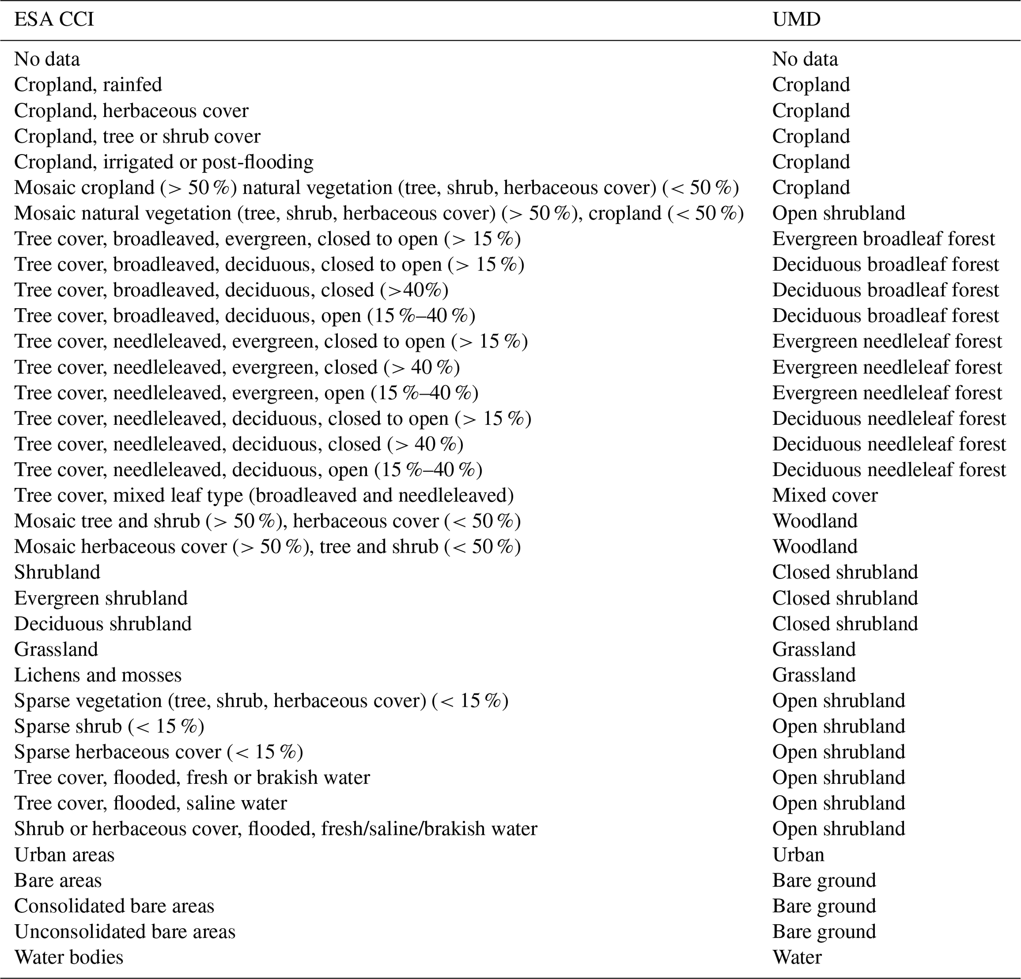
The LIS source code and default input parameters are available via https://lis.gsfc.nasa.gov (Kumar, 2021).
The updated vegetation, land cover and soil parameters, as well as validation datasets are available online, as documented in Sect. 2. The Monte Buey soil moisture data can be obtained from the Comisión Nacional de Actividades Espaciales (CONAE) upon request. The LIS simulation output can be obtained via https://doi.org/10.5281/zenodo.5091408 (Maertens et al., 2021).
MM performed the model simulations, produced figures and wrote the paper. GJMDL and SA contributed to the experiment setup and the writing of the paper. SVK and SPPM provided relevant input data for the simulations and contributed to the writing of the paper.
The authors declare that they have no conflict of interest.
Publisher's note: Copernicus Publications remains neutral with regard to jurisdictional claims in published maps and institutional affiliations.
The authors thank Mark Thibeault (CONAE) for providing the Monte Buey soil moisture data and David Mocko and Randy Koster for insightful discussions. We thank Clément Albergel and one anonymous reviewer for their very thorough and excellent reviews.
This study was performed within the framework of the Belgian Science Policy (BELSPO) project REFOR15 CHA (SR/00/338), with support of the Flemish Research Foundation (FWO 1512817N), C1 KU Leuven (C14/16/045) and the High Performance Computing system of the Vlaams Supercomputer Centrum.
This paper was edited by Wouter Buytaert and reviewed by Clément Albergel and one anonymous referee.
Albergel, C., Balsamo, G., de Rosnay, P., Muñoz-Sabater, J., and Boussetta, S.: A bare ground evaporation revision in the ECMWF land-surface scheme: evaluation of its impact using ground soil moisture and satellite microwave data, Hydrol. Earth Syst. Sci., 16, 3607–3620, https://doi.org/10.5194/hess-16-3607-2012, 2012. a, b
Albergel, C., Munier, S., Leroux, D. J., Dewaele, H., Fairbairn, D., Barbu, A. L., Gelati, E., Dorigo, W., Faroux, S., Meurey, C., Le Moigne, P., Decharme, B., Mahfouf, J.-F., and Calvet, J.-C.: Sequential assimilation of satellite-derived vegetation and soil moisture products using SURFEX_v8.0: LDAS-Monde assessment over the Euro-Mediterranean area, Geosci. Model Dev., 10, 3889–3912, https://doi.org/10.5194/gmd-10-3889-2017, 2017. a
Alton, P.: A simple retrieval of ground albedo and vegetation absorptance from MODIS satellite data for parameterisation of global land-surface models, Agr. Forest Meteorol., 149, 1769–1775, 2009. a
Amdan, M., Aragón, R., Jobbágy, E., Volante, J., and Paruelo, J.: Onset of deep drainage and salt mobilization following forest clearing and cultivation in the Chaco plains (Argentina), Water Resour. Res., 49, 6601–6612, 2013. a
Balsamo, G., Beljaars, A., Scipal, K., Viterbo, P., van den Hurk, B., Hirschi, M., and Betts, A. K.: A revised hydrology for the ECMWF model: Verification from field site to terrestrial water storage and impact in the Integrated Forecast System, J. Hydrometeorol., 10, 623–643, 2009. a
Barbu, A. L., Calvet, J.-C., Mahfouf, J.-F., Albergel, C., and Lafont, S.: Assimilation of Soil Wetness Index and Leaf Area Index into the ISBA-A-gs land surface model: grassland case study, Biogeosciences, 8, 1971–1986, https://doi.org/10.5194/bg-8-1971-2011, 2011. a
Barbu, A. L., Calvet, J.-C., Mahfouf, J.-F., and Lafont, S.: Integrating ASCAT surface soil moisture and GEOV1 leaf area index into the SURFEX modelling platform: a land data assimilation application over France, Hydrol. Earth Syst. Sci., 18, 173–192, https://doi.org/10.5194/hess-18-173-2014, 2014. a
Baret, F., Weiss, M., Lacaze, R., Camacho, F., Makhmara, H., Pacholcyzk, P., and Smets, B.: GEOV1: LAI and FAPAR essential climate variables and FCOVER global time series capitalizing over existing products. Part 1: Principles of development and production, Remote Sens. Environ., 137, 299–309, 2013. a
Bonan, G. B., Levis, S., Kergoat, L., and Oleson, K. W.: Landscapes as patches of plant functional types: An integrating concept for climate and ecosystem models, Global Biogeochem. Cy., 16, 5–1–5-23, 2002a. a
Bonan, G. B., Oleson, K. W., Vertenstein, M., Levis, S., Zeng, X., Dai, Y., Dickinson, R. E., and Yang, Z.-L.: The land surface climatology of the Community Land Model coupled to the NCAR Community Climate Model, J. Climate, 15, 3123–3149, 2002b. a
Bontemps, S., Herold, M., Kooistra, L., van Groenestijn, A., Hartley, A., Arino, O., Moreau, I., and Defourny, P.: Revisiting land cover observation to address the needs of the climate modeling community, Biogeosciences, 9, 2145–2157, https://doi.org/10.5194/bg-9-2145-2012, 2012. a
Boussetta, S., Balsamo, G., Beljaars, A., Kral, T., and Jarlan, L.: Impact of a satellite-derived leaf area index monthly climatology in a global numerical weather prediction model, Int. J. Remote Sens., 34, 3520–3542, 2013. a
Boussetta, S., Balsamo, G., Dutra, E., Beljaars, A., and Albergel, C.: Assimilation of surface albedo and vegetation states from satellite observations and their impact on numerical weather prediction, Remote Sens. Environ., 163, 111–126, 2015. a
Brocca, L., Tarpanelli, A., Filippucci, P., Dorigo, W., Zaussinger, F., Gruber, A., and Fernández-Prieto, D.: How much water is used for irrigation? A new approach exploiting coarse resolution satellite soil moisture products, Int. J. Appl. Earth Obs. Geoinf., 73, 752–766, 2018. a
Cao, Q., Yu, D., Georgescu, M., Han, Z., and Wu, J.: Impacts of land use and land cover change on regional climate: A case study in the agro-pastoral transitional zone of China, Environ. Res. Lett., 10, 124025, https://doi.org/10.1088/1748-9326/10/12/124025, 2015. a
Case, J. L., LaFontaine, F. J., Bell, J. R., Jedlovec, G. J., Kumar, S. V., and Peters-Lidard, C. D.: A real-time MODIS vegetation product for land surface and numerical weather prediction models, IEEE T. Geosci. Remote, 52, 1772–1786, 2013. a, b, c
Chadburn, S. E., Burke, E. J., Essery, R. L. H., Boike, J., Langer, M., Heikenfeld, M., Cox, P. M., and Friedlingstein, P.: Impact of model developments on present and future simulations of permafrost in a global land-surface model, The Cryosphere, 9, 1505–1521, https://doi.org/10.5194/tc-9-1505-2015, 2015. a
Chen, S., Su, H., and Zhan, J.: Estimating the impact of land use change on surface energy partition based on the Noah model, Front. Earth Sci., 8, 18–31, 2014. a
Chen, X., Zhang, Z., Chen, X., and Shi, P.: The impact of land use and land cover changes on soil moisture and hydraulic conductivity along the karst hillslopes of southwest China, Environ. Earth Sci., 59, 811–820, 2009. a
Clark, M. L., Aide, T. M., Grau, H. R., and Riner, G.: A scalable approach to mapping annual land cover at 250 m using MODIS time series data: A case study in the Dry Chaco ecoregion of South America, Remote Sens. Environ., 114, 2816–2832, 2010. a
Clark, M. P., Fan, Y., Lawrence, D. M., Adam, J. C., Bolster, D., Gochis, D. J., Hooper, R. P., Kumar, M., Leung, L. R., Mackay, D. S., Maxwell, R. M., Shen, C., Swenson, S. C., and Zeng, X.: Improving the representation of hydrologic processes in Earth System Models, Water Resour. Res., 51, 5929–5956, 2015. a, b, c
Cosby, B., Hornberger, G., Clapp, R., and Ginn, T.: A statistical exploration of the relationships of soil moisture characteristics to the physical properties of soils, Water Resour. Res., 20, 682–690, 1984. a, b
Crawford, T. M., Stensrud, D. J., Mora, F., Merchant, J. W., and Wetzel, P. J.: Value of incorporating satellite-derived land cover data in MM5/PLACE for simulating surface temperatures, J. Hydrometeorol., 2, 453–468, 2001. a
Csiszar, I. and Gutman, G.: Mapping global land surface albedo from NOAA AVHRR, J. Geophys. Res.-Atmos., 104, 6215–6228, 1999. a
Dai, Y., Shangguan, W., Wei, N., Xin, Q., Yuan, H., Zhang, S., Liu, S., Lu, X., Wang, D., and Yan, F.: A review of the global soil property maps for Earth system models, Soil, 5, 137–158, 2019. a, b
De Lannoy, G. J., Reichle, R. H., and Pauwels, V. R.: Global calibration of the GEOS-5 L-band microwave radiative transfer model over nonfrozen land using SMOS observations, J. Hydrometeorol., 14, 765–785, 2013. a
De Lannoy, G. J., Koster, R. D., Reichle, R. H., Mahanama, S. P., and Liu, Q.: An updated treatment of soil texture and associated hydraulic properties in a global land modeling system, J. Adv. Modeling Earth Syst., 6, 957–979, 2014. a, b, c, d, e, f, g
De Lannoy, G. J., Reichle, R. H., Peng, J., Kerr, Y., Castro, R., Kim, E. J., and Liu, Q.: Converting between SMOS and SMAP level-1 brightness temperature observations over nonfrozen land, IEEE Geosci. Remote Sens. Lett., 12, 1908–1912, 2015. a
de Queiroz, M. G., da Silva, T. G. F., Zolnier, S., Jardim, A. M. D. R. F., de Souza, C. A. A., Júnior, G. D. N. A., de Morais, J. E. F., and de Souza, L. S. B.: Spatial and temporal dynamics of soil moisture for surfaces with a change in land use in the semi-arid region of Brazil, Catena, 188, 104457, https://doi.org/10.1016/j.catena.2020.104457, 2020. a
Dickinson, R. E.: Land processes in climate models, Remote Sens. Environ., 51, 27–38, 1995. a
Ducharne, A., Koster, R. D., Suarez, M. J., Stieglitz, M., and Kumar, P.: A catchment-based approach to modeling land surface processes in a general circulation model: 2. Parameter estimation and model demonstration, J. Geophys. Res.-Atmos., 105, 24823–24838, 2000. a, b
Ek, M., Mitchell, K., Lin, Y., Rogers, E., Grunmann, P., Koren, V., and Gayno, G.: Implementation of Noah Land Surface Model Advances in the National Centers for Environmental Prediction Operational Mesoscale Eta Model, J. Geophys. Res., 108, 8851, https://doi.org/10.1029/2002JD003296, 2003. a, b
Entekhabi, D., Reichle, R. H., Koster, R. D., and Crow, W. T.: Performance metrics for soil moisture retrievals and application requirements, J. Hydrometeorol., 11, 832–840, 2010. a
ESA, L. C. C.: Product User Guide Version 2.0 (2017), available at: http://www.esa-landcover-cci.org (last access: 15 September 2020), 2017. a, b
FAO: The FAO-Unesco Soil Map of the World, Legend and 9 volumes, Unesco, Paris, France, 1971. a, b
FAO and ISRIC: JRC: Harmonized World Soil Database (version 1.2), FAO, Rome, Italy and IIASA, Laxenburg, Austria, 2012. a, b
Feldman, A. F., Akbar, R., and Entekhabi, D.: Characterization of higher-order scattering from vegetation with SMAP measurements, Remote Sens. Environ., 219, 324–338, 2018. a
Ge, Q., Zhang, X., and Zheng, J.: Simulated effects of vegetation increase/decrease on temperature changes from 1982 to 2000 across the Eastern China, Int. J. Climatol., 34, 187–196, 2014. a
Gelaro, R., McCarty, W., Suárez, M. J., Todling, R., Molod, A., Takacs, L., Randles, C. A., Darmenov, A., Bosilovich, M. G., Reichle, R., Wargan, K., Coy, L., Cullather, R., Draper, C., Akella, S., Buchard, V., Conaty, A., da Silva, A. M., Gu, W., Kim, G.-K., Koster, R., Lucchesi, R., Merkova, D., Nielsen, J. E., Partyka, G., Pawson, S., Putman, W., Rienecker, M., Schubert, S. D., Sienkiewicz, M., and Zhao, B.: The modern-era retrospective analysis for research and applications, version 2 (MERRA-2), J. Climate, 30, 5419–5454, 2017. a
Giménez, R., Mercau, J., Nosetto, M., Páez, R., and Jobbágy, E.: The ecohydrological imprint of deforestation in the semiarid Chaco: insights from the last forest remnants of a highly cultivated landscape, Hydrol. Process., 30, 2603–2616, 2016. a, b, c, d, e
Girotto, M., De Lannoy, G. J., Reichle, R. H., Rodell, M., Draper, C., Bhanja, S. N., and Mukherjee, A.: Benefits and pitfalls of GRACE data assimilation: A case study of terrestrial water storage depletion in India, Geophys. Res. Lett., 44, 4107–4115, 2017. a
Grossman-Clarke, S., Zehnder, J. A., Loridan, T., and Grimmond, C. S. B.: Contribution of land use changes to near-surface air temperatures during recent summer extreme heat events in the Phoenix metropolitan area, J. Appl. Meteorol. Clim., 49, 1649–1664, 2010. a
Gutman, G. and Ignatov, A.: The derivation of the green vegetation fraction from NOAA/AVHRR data for use in numerical weather prediction models, Int. J. Remote Sens., 19, 1533–1543, 1998. a, b, c, d
Han, X., Franssen, H.-J. H., Montzka, C., and Vereecken, H.: Soil moisture and soil properties estimation in the Community Land Model with synthetic brightness temperature observations, Water Resour. Res., 50, 6081–6105, 2014. a
Hansen, M. C., DeFries, R. S., Townshend, J. R., and Sohlberg, R.: Global land cover classification at 1 km spatial resolution using a classification tree approach, Int. J. Remote Sens., 21, 1331–1364, 2000. a
Hansen, M. C., Potapov, P. V., Moore, R., Hancher, M., Turubanova, S. A., Tyukavina, A., Thau, D., Stehman, S., Goetz, S. J., Loveland, T. R., Kommareddy, A., Egorov, A., Chini, L., Justice, C., and Townshend, J.: High-resolution global maps of 21st-century forest cover change, Science, 342, 850–853, 2013. a, b
Hengl, T., de Jesus, J. M., Heuvelink, G. B., Gonzalez, M. R., Kilibarda, M., Blagotic, A., Shangguan, W., Wright, M. N., Geng, X., Bauer-Marschallinger, B., Guevara, M. A., Vargas, R., MacMillan, R. A., Batjes, N., Leenaars, J., Carvalho Ribeiro, E., Wheeler, I., Mantel, S., and Kempen, B.: SoilGrids250m: Global gridded soil information based on machine learning, PLoS One, 12, e0169748, https://doi.org/10.1371/journal.pone.0169748, 2017. a
Houspanossian, J., Giménez, R., Jobbágy, E., and Nosetto, M.: Surface albedo raise in the South American Chaco: Combined effects of deforestation and agricultural changes, Agr. Forest Meteorol., 232, 118–127, 2017. a
INTA: Sistema De Información y Gestión Agrometeorológica, Instituto Nacional de Tecnologíca Agropecuaria, available at: http://siga2.inta.gov.ar/#/, last access: 15 January 2020. a
James, K. A., Stensrud, D. J., and Yussouf, N.: Value of real-time vegetation fraction to forecasts of severe convection in high-resolution models, Weather Forecast., 24, 187–210, 2009. a
Jarlan, L., Balsamo, G., Lafont, S., Beljaars, A., Calvet, J.-C., and Mougin, E.: Analysis of leaf area index in the ECMWF land surface model and impact on latent heat and carbon fluxes: Application to West Africa, J. Geophys. Res.-Atmos., 113, D24117, https://doi.org/10.1029/2007JD009370, 2008. a
Jiang, L., Kogan, F. N., Guo, W., Tarpley, J. D., Mitchell, K. E., Ek, M. B., Tian, Y., Zheng, W., Zou, C.-Z., and Ramsay, B. H.: Real-time weekly global green vegetation fraction derived from advanced very high resolution radiometer-based NOAA operational global vegetation index (GVI) system, J. Geophys. Res.-Atmos., 115, D11114, https://doi.org/10.1029/2009JD013204, 2010. a, b
Jobbágy, E. G., Giménez, R., Marchesini, V., Diaz, Y., Jayawickreme, D. H., and Nosetto, M. D.: Salt Accumulation and Redistribution in the Dry Plains of Southern South America: Lessons from Land Use Changes, in: Saline and Alkaline Soils in Latin America, Springer Nature, Cham, Switzerland, 51–70, 2020. a
Kaufmann, R. K., Zhou, L., Knyazikhin, Y., Shabanov, V., Myneni, R. B., and Tucker, C. J.: Effect of orbital drift and sensor changes on the time series of AVHRR vegetation index data, IEEE T. Geosci. Remote, 38, 2584–2597, 2000. a
Kirches, G., Brockmann, C., Boettcher, M., Peters, M., Bontemps, S., Lamarche, C., Schlerf, M., Santoro, M., and Defourny, P.: Land Cover CCI-Product User Guide-Version 2, available at: http://maps.elie.ucl.ac.be/CCI/viewer/download/ESACCI-LC-PUG-v2.5.pdf (last access: 15 September 2020), 2014. a, b, c
Kishné, A. S., Yimam, Y. T., Morgan, C. L., and Dornblaser, B. C.: Evaluation and improvement of the default soil hydraulic parameters for the Noah Land Surface Model, Geoderma, 285, 247–259, 2017. a, b
Knyazikhin, Y., Martonchik, J., Myneni, R. B., Diner, D., and Running, S. W.: Synergistic algorithm for estimating vegetation canopy leaf area index and fraction of absorbed photosynthetically active radiation from MODIS and MISR data, J. Geophys. Res.-Atmos., 103, 32257–32275, 1998. a
Koster, R.: “Efficiency space”: A framework for evaluating joint evaporation and runoff behavior, B. Am. Meteorol. Soc., 96, 393–396, 2015. a
Koster, R. D., Suarez, M. J., Ducharne, A., Stieglitz, M., and Kumar, P.: A catchment-based approach to modeling land surface processes in a general circulation model: 1. Model structure, J. Geophys. Res.-Atmos., 105, 24809–24822, 2000. a
Koster, R. D., Guo, Z., Yang, R., Dirmeyer, P. A., Mitchell, K., and Puma, M. J.: On the nature of soil moisture in land surface models, J. Climate, 22, 4322–4335, 2009. a
Koster, R. D. and Mahanama, P. P. S.: Land surface controls on hydroclimatic means and variability, J. Hydrometeorol., 13, 1604–1620, 2012. a
Kumar, S.: LIS Framework, available at: https://lis.gsfc.nasa.gov/, last access: 15 July 2021. a
Kumar, A., Chen, F., Barlage, M., Ek, M. B., and Niyogi, D.: Assessing impacts of integrating MODIS vegetation data in the weather research and forecasting (WRF) model coupled to two different canopy-resistance approaches, J. Appl. Meteorol. Clim., 53, 1362–1380, 2014. a
Kumar, S., Holmes, T., Mocko, D., Wang, S., and Peters-Lidard, C.: Attribution of flux partitioning variations between land surface models over the continental us, Remote Sens., 10, 751, https://doi.org/10.3390/rs10050751, 2018. a
Kumar, S. V., Peters-Lidard, C. D., Tian, Y., Houser, P. R., Geiger, J., Olden, S., Lighty, L., Eastman, J. L., Doty, B., Dirmeyer, P., Adams, J., Mitchell, K., Wood, E. F., and Sheffield, J.: Land information system: An interoperable framework for high resolution land surface modeling, Environ. Model. Softw., 21, 1402–1415, 2006. a
Kumar, S. V., Peters-Lidard, C. D., Eastman, J. L., and Tao, W.-K.: An integrated high-resolution hydrometeorological modeling testbed using LIS and WRF, Environ. Model. Softw., 23, 169–181, 2008. a
Kumar, S. V., Peters-Lidard, C. D., Santanello, J. A., Reichle, R. H., Draper, C. S., Koster, R. D., Nearing, G., and Jasinski, M. F.: Evaluating the utility of satellite soil moisture retrievals over irrigated areas and the ability of land data assimilation methods to correct for unmodeled processes, Hydrol. Earth Syst. Sci., 19, 4463–4478, https://doi.org/10.5194/hess-19-4463-2015, 2015. a
Kumar, S. V., M. Mocko, D., Wang, S., Peters-Lidard, C. D., and Borak, J.: Assimilation of Remotely Sensed Leaf Area Index into the Noah-MP Land Surface Model: Impacts on Water and Carbon Fluxes and States over the Continental United States, J. Hydrometeorol., 20, 1359–1377, 2019. a
Lawrence, D. M., Thornton, P. E., Oleson, K. W., and Bonan, G. B.: The partitioning of evapotranspiration into transpiration, soil evaporation, and canopy evaporation in a GCM: Impacts on land–atmosphere interaction, J. Hydrometeorol., 8, 862–880, 2007. a
Liang, S., Zhao, X., Liu, S., Yuan, W., Cheng, X., Xiao, Z., Zhang, X., Liu, Q., Cheng, J., Tang, H., Qu, Y., Bo, Y., Qu, Y., Ren, H., Yu, K., and Townshend, J.: A long-term Global LAnd Surface Satellite (GLASS) data-set for environmental studies, Int. J. Digit. Earth, 6, 5–33, 2013. a, b, c, d, e
Maertens, M., De Lannoy, G. J. M., Apers, S., Kumar, S. V., and Mahanama, S. P. P.: Land Surface modeling over the Dry Chaco: the impact of model structures, and soil, vegetation and land cover parameters, Zenodo, https://doi.org/10.5281/zenodo.5091408, 2021. a
Magliano, P. N., Fernández, R. J., Florio, E. L., Murray, F., and Jobbágy, E. G.: Soil physical changes after conversion of woodlands to pastures in Dry Chaco Rangelands (Argentina), Rangeland Ecol. Manage., 70, 225–229, 2017. a, b, c
Marchesini, V. A., Giménez, R., Nosetto, M. D., and Jobbágy, E. G.: Ecohydrological transformation in the Dry Chaco and the risk of dryland salinity: Following Australia's footsteps?, Ecohydrology, 10, e1822, https://doi.org/10.1002/eco.1822, 2017. a, b, c, d, e
Marchesini, V. A., Nosetto, M. D., Houspanossian, J., and Jobbágy, E. G.: Contrasting hydrological seasonality with latitude in the South American Chaco: The roles of climate and vegetation activity, J. Hydrol., 587, 124933, https://doi.org/10.1016/j.jhydrol.2020.124933, 2020. a, b
Martens, B., Miralles, D. G., Lievens, H., van der Schalie, R., de Jeu, R. A. M., Fernández-Prieto, D., Beck, H. E., Dorigo, W. A., and Verhoest, N. E. C.: GLEAM v3: satellite-based land evaporation and root-zone soil moisture, Geosci. Model Dev., 10, 1903–1925, https://doi.org/10.5194/gmd-10-1903-2017, 2017. a
Miller, J., Barlage, M., Zeng, X., Wei, H., Mitchell, K., and Tarpley, D.: Sensitivity of the NCEP/Noah land surface model to the MODIS green vegetation fraction data set, Geophys. Res. Lett., 33, L13404, https://doi.org/10.1029/2006GL026636, 2006. a, b
Minetti, J. L., Albarracín, S. A., Bobba, M. E., Hernández, C. M., López, E. R., Acuña, L. A., Costa, M. C., Nieva, I. J., and Mendoza, E.: Atlas climático del noroeste argentino, Instituto Nacional de Tecnología Agropecuaria, Santiago Del Estero, Argentina, 1999. a, b
Miralles, D. G., Holmes, T. R. H., De Jeu, R. A. M., Gash, J. H., Meesters, A. G. C. A., and Dolman, A. J.: Global land-surface evaporation estimated from satellite-based observations, Hydrol. Earth Syst. Sci., 15, 453–469, https://doi.org/10.5194/hess-15-453-2011, 2011. a
Morgan, C. L., Yimam, Y. T., Barlage, M., Gochis, D., and Dornblaser, B.: Valuing of soil capability in land surface modeling, in: Global Soil Security, Springer, , Cham, Switzerland, 53–61, 2017. a
Nosetto, M. D., Jobbágy, E., Brizuela, A. B., and Jackson, R.: The hydrologic consequences of land cover change in central Argentina, Agricult. Ecosyst. Environ., 154, 2–11, 2012. a, b, c
Oleson, K., Dai, Y., Bonan, G., Bosilovich, M., Dickinson, R., Dirmeyer, P., Hoffman, F., Houser, P., Levis, S., Niu, G., and Thornton, P.: Technical description of the community land model (CLM), NCAR Technical Note, NCAR, Boulder, USA, 2004. a
Oleson, K. W., Bonan, G. B., Schaaf, C., Gao, F., Jin, Y., and Strahler, A.: Assessment of global climate model land surface albedo using MODIS data, Geophys. Res. Lett., 30, 1443, https://doi.org/10.1029/2002GL016749, 2003. a
O'Neill, P., Njoku, E., Jackson, T., Chan, S., and Bindlish, R.: SMAP algorithm theoretical basis document: Level 2 & 3 soil moisture (passive) data products, JPL D-66480, Jet Propulsion Lab., California Inst. Technol., Pasadena, CA, USA, 2015. a
Peters-Lidard, C. D., Houser, P. R., Tian, Y., Kumar, S. V., Geiger, J., Olden, S., Lighty, L., Doty, B., Dirmeyer, P., Adams, J., Mitchell, K., Wood, E. F., and Sheffield, J.: High-performance Earth system modeling with NASA/GSFC's Land Information System, Innov. Syst. Softw. Eng., 3, 157–165, 2007. a
Pinzon, J. E. and Tucker, C. J.: A non-stationary 1981–2012 AVHRR NDVI3g time series, Remote Sens., 6, 6929–6960, 2014. a, b
Pitman, A. J.: The evolution of, and revolution in, land surface schemes designed for climate models, Int. J. Climatol., 23, 479–510, 2003. a
Pitman, A. J., de Noblet-Ducoudré, N., Cruz, F., Davin, E. L., Bonan, G., Brovkin, V., Claussen, M., Delire, C., Ganzeveld, L., Gayler, V., van den Hurk, B. J. J. M., Lawrence, P.J., van der Molen, M. K., Müller, C., Reick, C. H., Seneviratne, S. I., Strengers, B. J., and Voldoire, A.: Uncertainties in climate responses to past land cover change: First results from the LUCID intercomparison study, Geophys. Res. Lett., 36, L14814, https://doi.org/10.1029/2009GL039076, 2009. a
Priestley, C. H. B. and Taylor, R.: On the assessment of surface heat flux and evaporation using large-scale parameters, Mon. Weather Rev., 100, 81–92, 1972. a
Quets, J., De Lannoy, G. J., Al Yaari, A., Chan, S., Cosh, M. H., Gruber, A., Reichle, R. H., Van der Schalie, R., and Wigneron, J.-P.: Uncertainty in soil moisture retrievals: An ensemble approach using SMOS L-band microwave data, Remote Sens. Environ., 229, 133–147, 2019. a
Reichle, R. H., Koster, R. D., De Lannoy, G. J., Forman, B. A., Liu, Q., Mahanama, S. P., and Touré, A.: Assessment and enhancement of MERRA land surface hydrology estimates, J. Climate, 24, 6322–6338, 2011. a
Reichle, R. H., Draper, C. S., Liu, Q., Girotto, M., Mahanama, S. P., Koster, R. D., and De Lannoy, G. J.: Assessment of MERRA-2 land surface hydrology estimates, J. Climate, 30, 2937–2960, 2017. a
Reichle, R. H., Liu, Q., Koster, R. D., Crow, W. T., De Lannoy, G. J., Kimball, J. S., Ardizzone, J. V., Bosch, D., Colliander, A., Cosh, M., Kolassa, J., Mahanama, S. P. P., Prueger, J., Starks, P., and Walker, J. P.: Version 4 of the SMAP Level-4 Soil Moisture Algorithm and Data Product, J. Adv. Model. Earth Syst., 11, 3106–3130, 2019. a
Rigden, A. J., Salvucci, G. D., Entekhabi, D., and Short Gianotti, D. J.: Partitioning evapotranspiration over the continental United States using weather station data, Geophys. Res. Lett., 45, 9605–9613, 2018. a
Ruiz-Vasquez, M., Arias, P. A., Martínez, J. A., and Espinoza, J. C.: Effects of Amazon basin deforestation on regional atmospheric circulation and water vapor transport towards tropical South America, Clim. Dynam., 54, 4169–4189, 2020. a
Sabater, J. M., Rüdiger, C., Calvet, J.-C., Fritz, N., Jarlan, L., and Kerr, Y.: Joint assimilation of surface soil moisture and LAI observations into a land surface model, Agr. Forest Meteorol., 148, 1362–1373, 2008. a
Sellers, P., Mintz, Y., Sud, Y. E. A., and Dalcher, A.: A simple biosphere model (SiB) for use within general circulation models, J. Atmos. Sci., 43, 505–531, 1986. a
Thibeault, M., Cáceres, J. M., Dadamia, D., Soldano, A. G., Quirno, M. U., Guerrieri, J. M., Edrosa, R., Palomeque, M., Romaldi, L., Pucheta, J., Mogadouro, J., De Luca, E., Bustos, S., Agüero, S., Pascual, I., and Mariotti, M.: Spatial and temporal analysis of the Monte Buey SAOCOM and SMAP core site, in: IEEE International Geoscience and Remote Sensing Symposium (IGARSS), 26 July 2015, Milan, Italy, 969–971, 2015. a
Tucker, C. J., Pinzon, J. E., Brown, M. E., Slayback, D. A., Pak, E. W., Mahoney, R., Vermote, E. F., and El Saleous, N.: An extended AVHRR 8-km NDVI dataset compatible with MODIS and SPOT vegetation NDVI data, Int. J. Remote Sens., 26, 4485–4498, 2005. a, b, c
Vallejos, M., Volante, J. N., Mosciaro, M. J., Vale, L. M., Bustamante, M. L., and Paruelo, J. M.: Transformation dynamics of the natural cover in the Dry Chaco ecoregion: a plot level geo-database from 1976 to 2012, J. Arid Environ., 123, 3–11, 2015. a, b, c, d, e
Villegas, J. C., Breshears, D. D., Zou, C. B., and Law, D. J.: Ecohydrological controls of soil evaporation in deciduous drylands: how the hierarchical effects of litter, patch and vegetation mosaic cover interact with phenology and season, J. Arid Environ., 74, 595–602, 2010. a
Wang, J. R. and Schmugge, T. J.: An Empirical Model for the Complex Dielectric Permittivity of Soils as a Function of Water Content, IEEE T. Geosci. Remote, GE-18, 288–295, 1980. a
Wang, K. and Dickinson, R. E.: A review of global terrestrial evapotranspiration: Observation, modeling, climatology, and climatic variability, Rev. Geophys., 50, RG2005, https://doi.org/10.1029/2011RG000373, 2012. a
Wei, H., Xia, Y., Mitchell, K. E., and Ek, M. B.: Improvement of the Noah land surface model for warm season processes: Evaluation of water and energy flux simulation, Hydrol. Process., 27, 297–303, 2013. a
Wiekenkamp, I., Huisman, J. A., Bogena, H. R., and Vereecken, H.: Effects of Deforestation on Water Flow in the Vadose Zone, Water, 12, 35, https://doi.org/10.3390/w12010035, 2020. a
Wood, E. F., Roundy, J. K., Troy, T. J., Van Beek, L., Bierkens, M. F., Blyth, E., de Roo, A., Döll, P., Ek, M., Famiglietti, J., Gochis, D., van de giesen, N., Houser, P., Jaffé, P., Kollet, S., Lehner, B., Lettenmaier, D. P., Peters-Lidard, C., Sivapalan, M., Sheffield, J., Wade, A., and Whitehead, P.: Hyperresolution global land surface modeling: Meeting a grand challenge for monitoring Earth's terrestrial water, Water Resour. Res., 47, W05301, https://doi.org/10.1029/2010WR010090, 2011. a
Wösten, J., Lilly, A., Nemes, A., and Le Bas, C.: Development and use of a database of hydraulic properties of European soils, Geoderma, 90, 169–185, 1999. a
Wösten, J., Pachepsky, Y. A., and Rawls, W.: Pedotransfer functions: bridging the gap between available basic soil data and missing soil hydraulic characteristics, J. Hydrol., 251, 123–150, 2001. a
Xiao, Z., Liang, S., Wang, J., Xiang, Y., Zhao, X., and Song, J.: Long-time-series global land surface satellite leaf area index product derived from MODIS and AVHRR surface reflectance, IEEE T. Geosci. Remote, 54, 5301–5318, 2016. a, b, c
Yin, J., Zhan, X., Zheng, Y., Hain, C. R., Ek, M., Wen, J., Fang, L., and Liu, J.: Improving Noah land surface model performance using near real time surface albedo and green vegetation fraction, Agr. Forest Meteorol., 218, 171–183, 2016. a, b
Zeng, X.: Global vegetation root distribution for land modeling, J. Hydrometeorol., 2, 525–530, 2001. a
Zhang, B., Xia, Y., Long, B., Hobbins, M., Zhao, X., Hain, C., Li, Y., and Anderson, M. C.: Evaluation and comparison of multiple evapotranspiration data models over the contiguous United States: Implications for the next phase of NLDAS (NLDAS-Testbed) development, Agr. Forest Meteorol., 280, 107810, https://doi.org/10.1016/j.agrformet.2019.107810, 2020. a
Zhao, H., Zeng, Y., Lv, S., and Su, Z.: Analysis of soil hydraulic and thermal properties for land surface modeling over the Tibetan Plateau, Earth Syst. Sci. Data, 10, 1031–1061, https://doi.org/10.5194/essd-10-1031-2018, 2018. a
Zhu, Z., Bi, J., Pan, Y., Ganguly, S., Anav, A., Xu, L., Samanta, A., Piao, S., Nemani, R., and Myneni, R.: Global data sets of vegetation leaf area index (LAI) 3g and fraction of photosynthetically active radiation (FPAR) 3g derived from global inventory modeling and mapping studies (GIMMS) normalized difference vegetation index (NDVI3g) for the period 1981 to 2011, Remote Sens., 5, 927–948, 2013. a
Zwieback, S., Colliander, A., Cosh, M. H., Martínez-Fernández, J., McNairn, H., Starks, P. J., Thibeault, M., and Berg, A.: Estimating time-dependent vegetation biases in the SMAP soil moisture product, Hydrol. Earth Syst. Sci., 22, 4473–4489, https://doi.org/10.5194/hess-22-4473-2018, 2018. a