A climatological benchmark for operational radar rainfall bias reduction

The presence of significant biases in real-time radar quantitative precipitation estimations (QPEs) limits its use in hydrometeorological forecasting systems. Here, we introduce CARROTS (Climatology-based Adjustments for Radar Rainfall in an OperaTional Setting), a set of fixed bias reduction factors, which vary per grid cell and day of the year. The factors are based on a historical set of 10 years of 5 min radar and reference rainfall data for the Netherlands. CARROTS is both operationally available and independent of real-time rain gauge availability and can thereby provide an alternative to current QPE adjustment practice. In addition, it can be used as benchmark for QPE algorithm development. We tested this method on the resulting rainfall estimates and discharge simulations for 12 Dutch catchments and polders. We validated the results against the operational mean field bias (MFB)-adjusted rainfall estimates and a reference dataset. This reference consists of the radar QPE, that combines an hourly MFB adjustment and a daily spatial adjustment using observations from 32 automatic and 319 manual rain gauges. Only the automatic gauges of this network are available in real time for the MFB adjustment. The resulting climatological correction factors show clear spatial and temporal patterns. Factors are higher away from the radars and higher from December through March than in other seasons, which is likely a result of sampling above the melting layer during the winter months. The MFB-adjusted QPE outperforms the CARROTS-corrected QPE when the country-average rainfall estimates are compared to the reference. However, annual rainfall sums from CARROTS are comparable to the reference and outperform the MFB-adjusted rainfall estimates for catchments away from the radars, where the MFB-adjusted QPE generally underestimates the rainfall amounts. This difference is absent for catchments closer to the radars. QPE underestimations are amplified when used in the hydrological model simulations. Discharge simulations using the QPE from CARROTS outperform those with the MFB-adjusted product for all but one basin. Moreover, the proposed factor derivation method is robust. It is hardly sensitive to leaving individual years out of the historical set and to the moving window length, given window sizes of more than a week.

1 Introduction

Radar rainfall estimates are essential for hydrometeorological forecasting systems. In these systems, the data are used to force hydrological models (e.g., Borga, 2002; Thorndahl et al., 2017), to initialize numerical weather prediction models (e.g., Haase et al., 2000; Rogers et al., 2000) or as input data for rainfall nowcasting techniques (e.g., Ebert et al., 2004; Wilson et al., 2010; Foresti et al., 2016; Heuvelink et al., 2020; Imhoff et al., 2020a). A major disadvantage of radar quantitative precipitation estimations (QPEs) are the considerable biases with respect to the true rainfall, caused by three main groups of errors: (1) sources of errors related to the reflectivity measurements, (2) sources of errors in the conversion from reflectivity to rainfall rate and (3) spatiotemporal sampling errors (Austin, 1987; Joss and Lee, 1995; Creutin et al., 1997; Gabella et al., 2000; Sharif et al., 2002; Uijlenhoet and Berne, 2008; Ochoa-Rodriguez et al., 2019; Imhoff et al., 2020b). These biases can be amplified when used in hydrological models (Borga, 2002; Borga et al., 2006; Brauer et al., 2016). Hence, radar QPE requires corrections before operational use in hydrometeorological (forecasting) models.

A large number of correction methods are already available. These methods range from corrections prior to the rainfall estimations, e.g., corrections for physical phenomena such as ground clutter, attenuation, the vertical profile of reflectivity (VPR) and variations in raindrop size distribution (e.g., Joss and Pittini, 1991; Germann and Joss, 2002; Berenguer et al., 2006; Cho et al., 2006; Uijlenhoet and Berne, 2008; Kirstetter et al., 2010; Qi et al., 2013; Hazenberg et al., 2013, 2014), to statistical post-processing steps for bias removal in the radar QPE using rain gauge data. These post-processing methods either merge rain gauge and radar QPE from the same interval or base correction factors on the total precipitation in both products over a past period, such as a number of rainy days (e.g., 7 d in Park et al., 2019). An often used method is the mean field bias (MFB) correction method, which determines a spatially averaged correction factor from the ratio between rain gauge observations and the radar QPE of the superimposed grid cells at the locations of these gauges (Smith and Krajewski, 1991; Seo et al., 1999). This method, which is used operationally in the Netherlands and many other countries (Holleman, 2007; Harrison et al., 2009; Thorndahl et al., 2014; Goudenhoofdt and Delobbe, 2016), does not account for any spatial variability in the radar QPE bias, even though the bias is known to increase with increasing distance from the radar (Koistinen and Puhakka, 1981; Joss and Lee, 1995; Koistinen et al., 1999; Gabella et al., 2000; Michelson and Koistinen, 2000; Seo et al., 2000).

It is possible to account for this spatial variability with geostatistical techniques (e.g., ordinary kriging, kriging with external drift or co-kriging; Krajewski, 1987; Creutin et al., 1988; Wackernagel, 2003; Schuurmans et al., 2007; Goudenhoofdt and Delobbe, 2009; Sideris et al., 2014) or Bayesian merging methods (Todini, 2001). Although these methods substantially improve the QPE in the spatial domain, all gauge-based radar QPE adjustment methods are limited by the timely availability of sufficient, and ideally quality-controlled, rain gauge observations (for an overview of methods and their limitations, see Ochoa-Rodriguez et al., 2019). The gauge networks operated by the Royal Netherlands Meteorological Institute (KNMI) are an example of this issue. Although there is approximately one station per 100 km², only 32 out of 351 rain gauges operate automatically. The remaining 319 manual rain gauges report just once a day. Thus, only the automatic rain gauges are used for the MFB adjustment that takes place every hour in real time (Holleman, 2007) and recently even every 5 min.

In addition, two potential operational (forecasting) issues need to be considered when using these more advanced geostatistical and Bayesian merging methods: (1) the methods are computationally expensive, especially methods such as co-kriging and Bayesian merging that integrate radar and rain gauges (Ochoa-Rodriguez et al., 2019), and (2) when the adjustment method changes the spatial structure of the original radar rainfall fields (kriging and Bayesian methods), this may impact the continuity of the rainfall fields over time and thereby also the radar rainfall nowcasts (Ochoa-Rodriguez et al., 2013; Na and Yoo, 2018). In the case that the nowcasts suffer from errors due to these adjustments, adjustment methods should be applied to the nowcasts as a post-processing step. To do this, the forecaster would need to estimate the future (bias) correction factors (a method for this using MFB adjustment is described in Seo et al., 1999) or simply assume that the latest correction factors are exemplary for the coming hours.

Hence, operational hydrometeorological forecasting calls for a radar rainfall adjustment approach that (1) takes the spatial variability in radar QPE errors into account and (2) is available in real time so that it can be used operationally for radar-based rainfall forecasts, such as nowcasting. Here, we present CARROTS (Climatology-based Adjustments for Radar Rainfall in an OperaTional Setting), a set of gridded climatological adjustment factors for every day of the year, based on a historical set of 10 years of 5 min radar and reference rainfall data for the Netherlands. When sufficient rain gauges are operationally available, which would allow for a robust application of more advanced geostatistical and Bayesian merging methods, CARROTS can serve as a benchmark for testing these and other more sophisticated adjustment techniques.

2 Data and methods

2.1 Radar rainfall estimates

The archive (2009–2018) of radar rainfall composites in this study originates from two C-band weather radars operated by KNMI (Fig. 1). Between September 2016 and January 2017, both radars were replaced by dual-polarization radars, and the radar in De Bilt (“DB” in Fig. 1) was replaced by a new one in Herwijnen (“H” in Fig. 1). The radar renewals and relocation have had a limited impact on the QPE product, mainly because the operational products are not yet (fully) using the additional information from the dual-polarization (Beekhuis and Holleman, 2008; Beekhuis and Mathijssen, 2018).

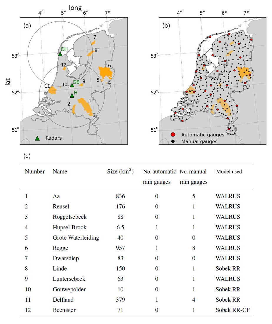
Figure 1 Overview of the basins in this study: (a) study area with the location of the three radars (green triangles) operated by KNMI and the 12 basins (orange polygons). The two grey circles indicate a range of 100 km around the radars in Den Helder (DH) and Herwijnen (H). The other radar (DB) is the radar in De Bilt, which was used until January 2017 and replaced by the radar in Herwijnen. Note that the range used in the composite was more than 100 km, but 100 km is often regarded as the distance up to which the radar QPE is expected to be reliable. (b) Locations of the 32 automatic and 319 manual rain gauges currently operated by KNMI. Note that the number of rain gauges has slightly changed from 2009 until present. (c) List of the basin names, sizes, number of gauges in the basin and hydrological models employed. The numbers in the left column refer to the numbers in (a). The right column states the used model for these areas.

The radar product is Doppler-filtered for ground clutter. This product is then used to construct horizontal cross-sections at a nearly constant altitude of 1500 m, called pseudo-constant plan position indicators (pseudo-CAPPIs). Subsequently, range-weighted compositing is used to combine the reflectivities from both radars (Overeem et al., 2009b). Since 2013, non-meteorological echoes have been removed as an additional step with a cloud mask obtained from satellite imagery. As a final step, rainfall rates are estimated with a fixed Z–R relationship (Marshall et al., 1955):

$$\begin{array}{}\text{(1)}& {\displaystyle }{\displaystyle }{Z}_{\mathrm{h}}=\mathrm{200}{R}^{\mathrm{1.6}}.\end{array}$$

In this equation, Z_h is the reflectivity at horizontal polarization (mm⁶ m⁻³ but generally given in dBZ, according to 10×log ₁₀[Z_h]), and R is the rainfall rate (mm h⁻¹). The final product is called the unadjusted radar QPE (R_U) in this study.

KNMI also provides adjusted radar rainfall products, based on the aforementioned product, but adjusted with quality-controlled observations from both 32 automatic hourly and 319 manual daily rain gauges (Overeem et al., 2009a, b, 2011; note that the number of rain gauges has slightly changed from 2009 until present). The same 32 automatic rain gauges are used for the MFB-adjustment method, which will be introduced in Sect. 2.2.1. In contrast to the spatially uniform hourly MFB adjustment, the observations from the manual rain gauges are used for daily spatial adjustments, based on distance-weighted interpolation of these observations (Barnes, 1964; Overeem et al., 2009b). See Sect. 2.2.3 for a more detailed description of this method.

This product is considered as a reference rainfall product in the Netherlands, and it is therefore also regarded as the reference here (referred to as R_A in this study). The R_A data are not available in real time (available with a delay of 1 to 2 months because they only use quality-controlled and validated rain gauge observations), but they are archived and can therefore be used for “offline” methods. Both R_A and R_U have a 1 km² spatial and 5 min temporal resolution.

Table 1 Statistics of Fig. 2. Indicated are the sample size, the slope of a linear fit between the two rainfall products (R_A and R_U; the dashed colored lines in Fig. 2) for all observations and the Pearson correlation coefficient. This is indicated per season (DJF is winter, MAM is spring, JJA is summer and SON is autumn) and for all seasons together (Total).

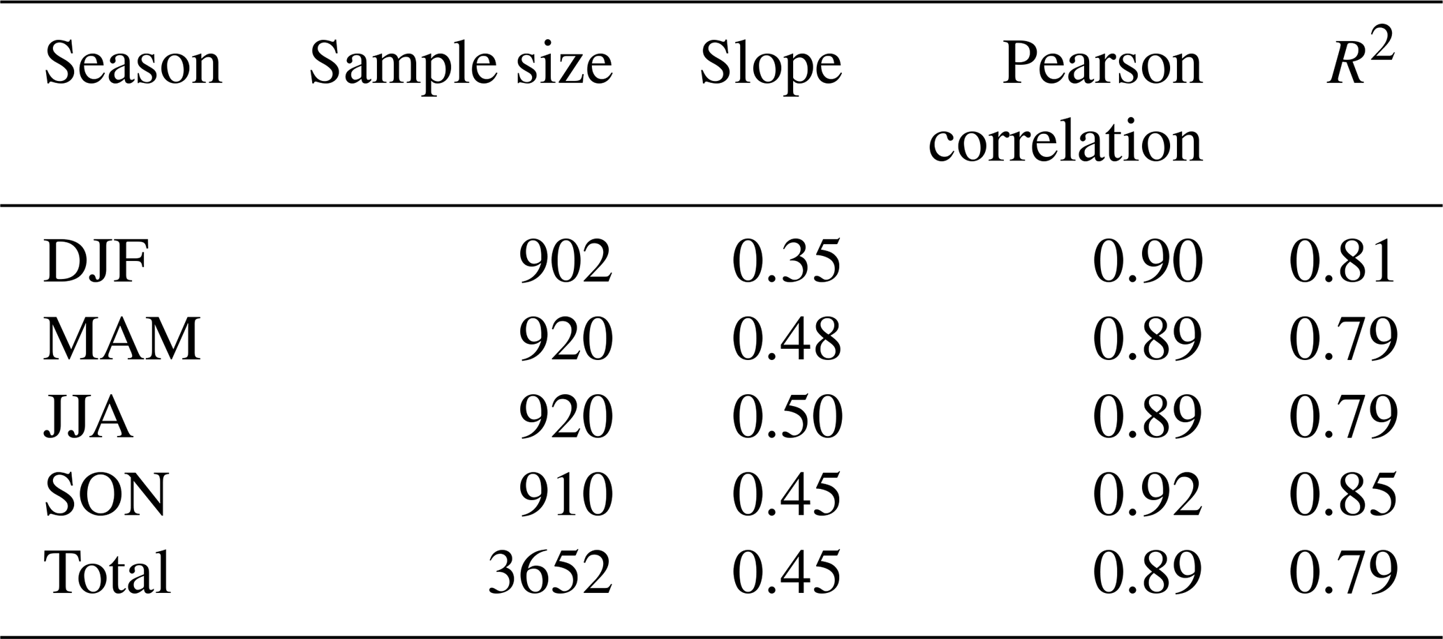
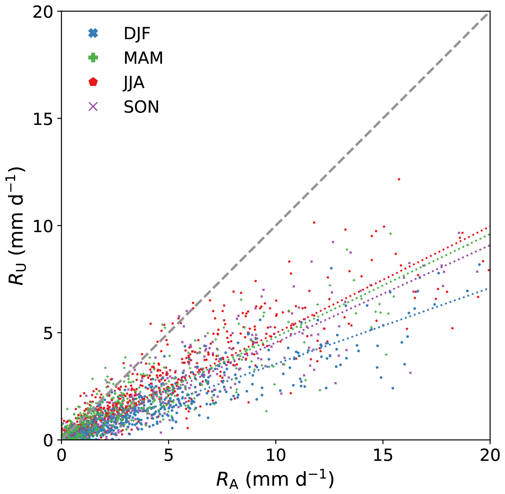
Figure 2 The systematic discrepancy between the reference rainfall (R_A) and the unadjusted radar QPE (R_U). Shown are the daily country-average rainfall sums based on 10 years (2009–2018), classified per season. The slope, Pearson correlation and sample size per season are indicated in Table 1. The dashed colored lines are a linear fit, forced through the origin, per season between R_A and R_U.

The year 2008 is actually the first year in the KNMI archive of both datasets, but it was left out of the analysis here. R_U for this year showed a significantly different behavior than the other years, especially during the first half year in which the product rarely underestimated and frequently even overestimated the rainfall sums. The reason for this behavior is not yet fully understood. KNMI (2009) reported that spring was exceptionally dry in the north of the country and that the months January and May were among the warmest on record. On some days with overestimations, clear bright band effects were visible in the radar mosaic, which may have contributed to the systematic differences.

2.2 Bias correction factors

Figure 2 indicates the need for correction of the real-time available radar rainfall product. R_U systematically underestimates the true rainfall amounts, averaged for the land surface area of the Netherlands, by 55 %. This bias is not uniform in space, as will be highlighted in Sect. 3, and in time with higher underestimations during winter (on average 65 %) than during the other seasons (50 %–55 %). In the following two subsections, the operationally used MFB-adjustment method and the CARROTS method proposed in this study will be introduced.

2.2.1 Mean field bias adjustment

The mean field bias (MFB) adjustment method is the operational adjustment technique in the Netherlands, and it was used in this study for comparison with the proposed climatological bias reduction method (Sect. 2.2.2). This method provides a spatially uniform multiplicative adjustment factor that is applied to R_U. The adjustment factor (F_MFB) was calculated as (Holleman, 2007; Overeem et al., 2009b)

$$\begin{array}{}\text{(2)}& {\displaystyle }{\displaystyle }{F}_{\text{MFB}}={\displaystyle \frac{\sum _{n=\mathrm{1}}^{N}G(i_n,j_n)}{\sum _{n=\mathrm{1}}^N{R}_{\mathrm{U}}(i_n,j_n)}},\end{array}$$

with G(i_n,j_n) the hourly rainfall sum for gauge n at location (i_n,j_n) and R_U(i_n,j_n) the unadjusted hourly rainfall sum for the corresponding radar grid cell. The calculation of F_MFB was only performed when both the rainfall sum of all rain gauges together and the sum of all corresponding radar grid cells were at least 1.0 mm. In all other cases, F_MFB=1.0.

The MFB-adjustment factors were determined from the 1 h accumulations of both R_U and the 32 automatic rain gauges, as only the automatic gauges were operationally available every hour (Holleman, 2007; Overeem et al., 2009b). The adjustment factors at the temporal resolution of the radar QPE (5 min) were assumed to equal the 1 h adjustment factors for a given hour.

Moreover, this analysis took place with archived datasets, which were validated and consisted of quality-controlled rain gauge observations. It is noteworthy that the same quality control is absent and that missing data occur in real time, which can lead to deteriorating results when the MFB adjustment is applied in an operational test case.

2.2.2 CARROTS method

To derive the climatological bias correction factors for the CARROTS method, both R_U and R_A were used for the years 2009–2018. The use of the reference data for this method was possible because the CARROTS method did not require a real-time availability of the data. The bias correction factors were determined per grid cell in the radar domain according to the following three steps:

1. For every day in the period 2009–2018, all 5 min rainfall sums (both R_U and R_A) within a moving window of 31 d (the day of interest plus the 15 d before and after it) were summed. The purpose of the moving window was to smooth the systematic day-to-day variability of the estimated rainfall in the 10-year data. Sections 2.4 and 3.4 describe a leave-one-year-out validation of the method, and they describe the sensitivity of the method to the moving window size.

2. For every day of the year, the 31 d sums around that day were averaged over the 10 years. Thus, the value for, e.g., 16 January consisted of the average 31 d sum for the period 1 to 31 January over the 10 years. Leap years are left out of this analysis due to the low number of leap years in the studied period.

3. Finally, gridded climatological adjustment factors (F_clim) were calculated per day of the year as

   $$\begin{array}{}\text{(3)}& {\displaystyle }{\displaystyle }{F}_{\text{clim}}(i,j)={\displaystyle \frac{R_{\mathrm{A}}(i,j)}{R_{\mathrm{U}}(i,j)}},\end{array}$$

   with R_A(i,j) the reference rainfall sum and R_U(i,j) the unadjusted (operational) radar rainfall sum at grid cell (i,j) for the 10 years.

2.2.3 Spatial adjustments for the reference product

The adjustment procedure to derive R_A consists of three steps: (1) mean field bias correction (one adjustment factor for the whole country which varies per hour; see Sect. 2.2.1), (2) derivation of a daily spatial adjustment factor per grid cell and (3) spatial adjustment of the hourly or higher frequency MFB-adjusted rainfall fields (step 1) using the spatial adjustment from step 2.

A spatial adjustment factor (step 2) is derived per grid cell as follows (for a more elaborate description, see Sect. 3 in Overeem et al., 2009a, b):

$$\begin{array}{}\text{(4)}& {\displaystyle }{\displaystyle }{F}_{\mathrm{S}}(i,j)={\displaystyle \frac{{\sum }_{n=\mathrm{1}}^N{w}_n(i,j)\cdot G(i_n,j_n)}{{\sum }_{n=\mathrm{1}}^N{w}_n(i,j)\cdot R_U(i_n,j_n)}},\end{array}$$

with N the number of radar–gauge pairs, G(i_n,j_n) the daily rainfall sum for manual rain gauge n at location (i_n,j_n) and R_U(i_n,j_n) the unadjusted daily rainfall sum for the corresponding radar grid cell. w_n(i,j) is a weight for gauge n, based on the following function:

$$\begin{array}{}\text{(5)}& {\displaystyle }{\displaystyle }{w}_n(i,j)=e^{-\frac{d_n^{\mathrm{2}}(i,j)}{{\mathit{\sigma }}^{\mathrm{2}}}}.\end{array}$$

Here, $d_n^{\mathrm{2}}(i,j)$ is the squared distance between gauge n and the grid cell for which the factor is derived. σ determines the smoothness of the adjustment factor field. It was set to 12 km by Overeem et al. (2009a, b), based on the average gauge spacing in the Netherlands.

Finally, to spatially adjust the hourly MFB-adjusted rainfall fields (step 3), two more steps are followed. First, the hourly MFB-adjusted rainfall fields (see Sect. 2.2.1 for the MFB-adjustment method) are accumulated to daily sums. For each grid cell, a new adjustment field is then determined:

$$\begin{array}{}\text{(6)}& {\displaystyle }{\displaystyle }{F}_{\text{MFBS}}(i,j)={\displaystyle \frac{R_S(i,j)}{R_{\text{MFB}}(i,j)}},\end{array}$$

with R_S(i,j) the spatially adjusted daily sum for grid cell (i,j) obtained using Eq. (4) and R_MFB(i,j) the MFB-adjusted daily sum for grid cell (i,j). Second, the 1 h or higher frequency (5 min in this study) MFB-adjusted rainfall fields are multiplied by the adjustment factor F_MFBS(i,j).

2.3 Hydrometeorological application

Both bias adjustment methods were applied to the 10 years (2009–2018) of R_U. In order to provide a hydrometeorological testbed, both the CARROTS and MFB-adjusted QPE products (from here on referred to as R_C and R_MFB, respectively) were validated against the reference rainfall. First, this was done at country level. The estimated daily rainfall sums for all grid cells within the land surface area of the Netherlands were compared to the reference in a similar way as the comparison in Fig. 2. To subdivide these results per year and season, an additional hourly rainfall sum validation was performed as well. The results of this analysis can be found in the Appendix, and the analysis was done as follows: for every rainy hour (when the sum of at least one grid cell was larger than 0.0 mm), we computed the root mean square error (RMSE) by squaring the differences between the three QPE products (R_U, R_C and R_MFB) on the one hand and the reference on the other and taking the average of these squared differences over all grid cells within the land surface area of the Netherlands. Subsequently, the RMSE was averaged over all rainy hours in that season and year. Finally, the seasonal mean RMSE was divided by the average hourly rainfall rate for that season and year, resulting in the fractional standard error (FSE) score. The FSE score was calculated for every season in the 10 years to be able to compare the seasonal performance of the hourly rainfall estimates of R_U, R_C and R_MFB.

Second, the annual rainfall sums for 12 basins (a combination of catchments and polders) in the Netherlands (Fig. 1) were compared with the reference. In addition, R_C and R_MFB were used as input for the rainfall-runoff models of the 12 basins. Most of the involved water authorities use these (lowland) rainfall-runoff models either operationally or for research purposes, often embedded in a Delft-FEWS system, which is a data-integration platform used worldwide by many hydrological forecasting agencies and water management organizations that brings data handling and model integration together for operational forecasting (Werner et al., 2013). For this reason, most models were already calibrated using interpolated rain gauge data or the R_A product (e.g. Brauer et al., 2014b; Sun et al., 2020). The calibration period was based on the availability and quality of discharge observations for that basin, but it was generally 1 to 2 years within the period considered in this study (2009–2018). The WALRUS models for catchments Roggelsebeek and Dwarsdiep were not calibrated prior to this study and were therefore calibrated with the reference data (R_A) for the periods 2013–2014 (Roggelsebeek) and 2016–2017 (Dwarsdiep). The choice for these periods was based on discharge observation availability and quality. The employed SOBEK RR(-CF) model (Stelling and Duinmeijer, 2003; Stelling and Verwey, 2006; Prinsen et al., 2010) is semi-distributed, and therefore we used sub-catchment-averaged rainfall sums from the gridded radar QPE. The four basins with a SOBEK model have the following number of sub-catchments: 7 for Gouwepolder, 1 for Beemster, 25 for Delfland and 23 for Linde. WALRUS (Brauer et al., 2014a) is lumped, so the catchment-averaged radar QPE was used as input. A more detailed description of both rainfall-runoff models is outside the scope of this paper. All 12 model setups were run with a 5 min time step for the period 2009–2018.

The resulting discharge simulations were validated for the same period and 5 min time step using the Kling–Gupta efficiency (KGE) metric (Gupta et al., 2009):

$$\begin{array}{}\text{(7)}& {\displaystyle }{\displaystyle }\text{KGE}=\mathrm{1}-\sqrt{(\mathit{\rho }-\mathrm{1}{)}^{\mathrm{2}}+(\mathit{\alpha }-\mathrm{1}{)}^{\mathrm{2}}+(\mathit{\beta }-\mathrm{1}{)}^{\mathrm{2}}},\end{array}$$

with

$$\begin{array}{}\text{(8)}& {\displaystyle }& {\displaystyle }\mathit{\alpha }={\displaystyle \frac{{\mathit{\sigma }}_{\mathrm{s}}}{{\mathit{\sigma }}_{\mathrm{o}}}},\text{(9)}& {\displaystyle }& {\displaystyle }\mathit{\beta }={\displaystyle \frac{{\mathit{\mu }}_{\mathrm{s}}}{{\mathit{\mu }}_{\mathrm{o}}}}.\end{array}$$

Here, ρ is the Pearson correlation between observed and simulated discharge, α the flow variability error between observed and simulated discharge and β the bias between mean simulated (μ_s) and mean observed (μ_o) discharge. σ_s and σ_o are the standard deviations of the simulated and observed discharge. The KGE metric ranges from −∞ to 1.0, with 1.0 representing a perfect agreement between observations and simulations. In this study, the discharge simulated with R_A as input was regarded as the observation.

Note that this validation method was not a leave-one-out or split-sample validation, as the full 10-year dataset was used for R_A and the CARROTS- and MFB-adjustment derivation, and shorter periods in those 10 years were used for hydrological model calibration. However, the sensitivity of the CARROTS factor was tested by leaving individual years out of the derivation period (Sect. 2.4).

2.4 Sensitivity analysis

As mentioned in Sect. 2.2.2, the purpose of the 31 d moving window in the factor derivation of CARROTS was to smooth the day-to-day variability of rainfall. To test the sensitivity of the method to the employed moving window size, the adjustment factors were re-derived for a range of moving window sizes (1 d, 1 week, 2 weeks, 6 weeks and 2 months). The derived factors were then compared to the original factor in this study, which was based on a moving window size of 31 d, and used to derive adjusted QPE products. Subsequently, these QPE products served as input for 1 of the 12 catchments, namely the WALRUS model for the Aa catchment (Fig. 1), to test the effect on the simulated discharges (see Sect. 3.4 and Fig. 8 for the results). The Aa catchment was chosen because the unadjusted QPE product (R_U) for this catchment has one of the highest biases of the 12 studied catchments (see Sect. 3 and Fig. 4).

Besides the moving window choice, the length of the radar rainfall archive (10 years) was finite. To test whether or not this archive length was sufficient for reaching a stable factor derivation, individual years in the 10-year archive were left out of the CARROTS method. Hence, the adjustment factors were recalculated 10 times in a leave-one-year-out method, applied to R_U and used as input for the WALRUS simulations for the Aa catchment. See Sect. 3.4 and Fig. 4 for the results.

3 Results

3.1 Seasonal and spatial variability

The adjustment factors from CARROTS present the spatial variability in the radar QPE errors, with generally higher adjustment factors towards the edges of the radar domain (Fig. 3). This difference is most pronounced from December through March, with factors in the south and east of the country more than 2 times higher than in the central and northwestern parts (Fig. 3a, b and l). Figure 3 demonstrates a clear annual cycle of the adjustment factors, with higher adjustment factors from December through March than in the other months. Figure 4a shows similar results for the catchment-averaged adjustment factors, with factors ranging from 2.1 for the Beemster polder to 3.2 for the Hupsel Brook catchment in January, whereas adjustment factors range from 1.3 for the Grote Waterleiding catchment to 1.6 for the Roggelsebeek catchment in June.

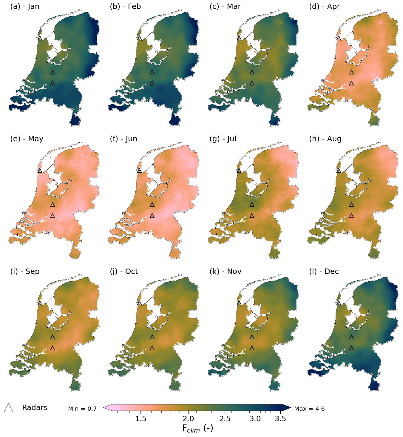
Figure 3 Spatial variability of the CARROTS factors, as derived from the archived radar and reference data for the period 2009–2018. Shown are monthly averages of the daily factors.

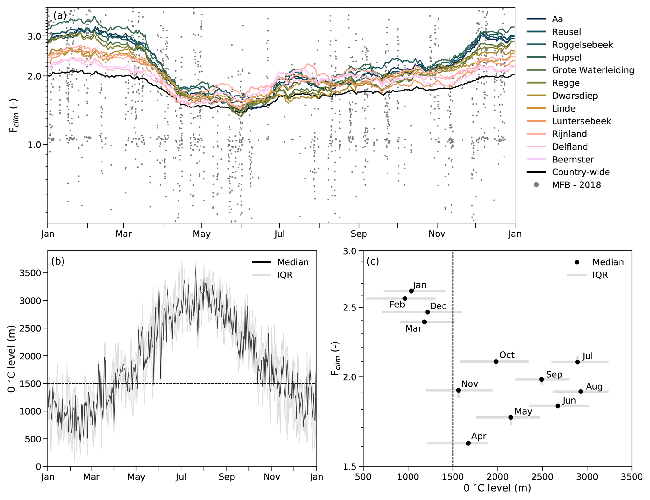
Figure 4 Seasonal dependency of the CARROTS factors and comparison with the operational MFB-adjustment factor. (a) Temporal variability of the climatological daily adjustment factors for the 12 basins (colors, catchment-averaged), the country-average (black line) and of the country-wide hourly MFB factor for the (example) year 2018 (grey dots; some also fall outside the indicated range). (b) Estimate of the height of the 0 ^∘C isotherm at KNMI station De Bilt for all rainy hours in the 10-year period, based on a constant wet adiabatic lapse rate of 5.5 K km⁻¹. (c) Dependency of the monthly adjustment factor on the estimated 0 ^∘C isotherm level for KNMI station De Bilt and the superimposed grid cell of this station. Depending on the location in the radar composite, the minimum CARROTS factor can take place in a different month but is always between April and June. Note that for this analysis, the adjustment factor was based on only the rainfall sums within that month, the “effective adjustment factor” for that month, which roughly coincides with the factor for the 15th of the month in the CARROTS method. The grey bars indicate the interquartile range (IQR) for that month, based on the spread in hourly 0 ^∘C isotherm level estimates (the horizontal bars) and the sensitivity to leaving out individual years in the 10-year period for the factor derivation (vertical bars).

An explanation for these higher adjustment factors from December through March is that radar QPE often severely underestimates the rainfall amounts for stratiform systems, which regularly occur during the Dutch winter. This especially holds when the QPE is constructed from reflectivities sampled above the melting layer (Fabry et al., 1992; Kitchen and Jackson, 1993; Germann and Joss, 2002; Bellon et al., 2005; Hazenberg et al., 2013). This seems to be the case here as well. A simple first-order estimation of the 0 ^∘C isotherm level, using a constant wet adiabatic lapse rate of 5.5 K km⁻¹ with ground temperature data for all rainy hours in the 10 years (Fig. 4b), indicates that the 1500 m pseudo-CAPPI is generally above the 0 ^∘C isotherm level from December through March. This coincides with the months with higher adjustment factors (Fig. 4c) and could thus explain the winter effect on the adjustment factors. This effect is presumably even stronger further away from the radars because the QPE product consists of samples at even higher altitudes than 1500 m for locations more than 120 km from the radars. Besides, an additional dependency of the monthly factor on the time of year that cannot be explained by temperature seems to be present, with lower adjustment factors during spring and early summer and higher factors for the subsequent period (Fig. 4c).

3.2 Evaluation of the rainfall sums

The MFB-adjusted QPE (R_MFB) significantly reduces the systematic bias of R_U (Fig. 2), from a 55 % underestimation on average for the Netherlands to 10 % (Fig. 5a and Table 2). However, the remaining bias in R_MFB is generally caused by a systematic underestimation of the reference rainfall. The overall underestimation is less for R_C (8 %, Fig. 5b) but results from estimation errors that are associated with either under- or overestimates of the reference rainfall. The spread in Fig. 5b is significantly wider than in Fig. 5a, indicating that the country-wide QPE error of R_C is often higher than for R_MFB. The yearly FSE in Table A1 clearly indicates this too, with a systematically higher FSE for R_C than for R_MFB.

Table 2 Statistics of Fig. 5. Indicated are the sample size, the Pearson correlation and the slope of a linear fit between the reference and the two adjusted radar QPE products (R_MFB and R_C; the dashed colored lines in Fig. 5). This is indicated per season and for all seasons together (Total).

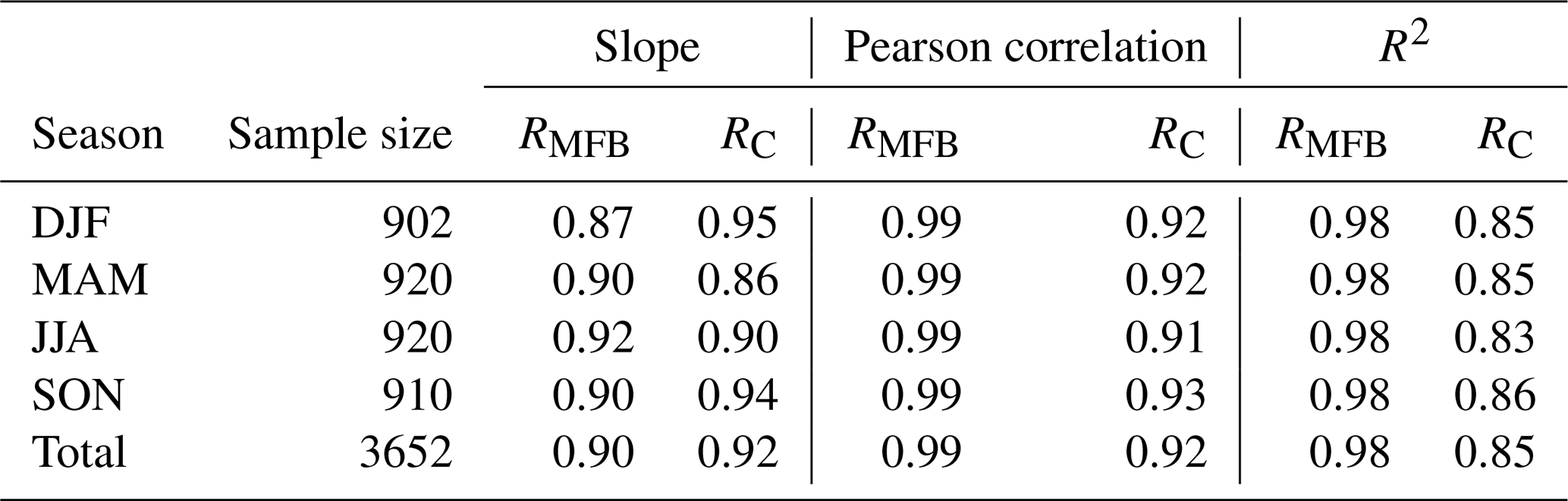
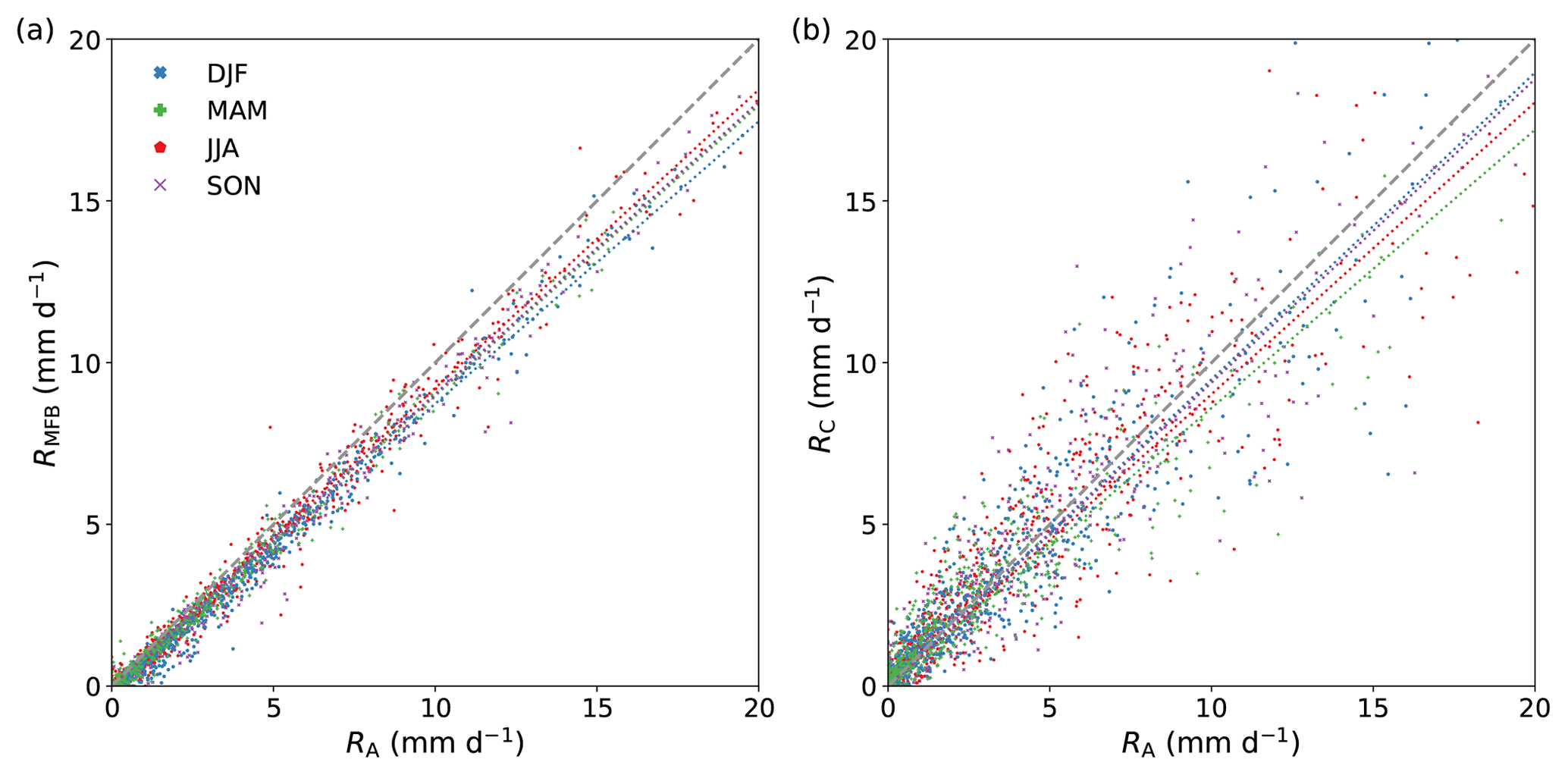
Figure 5 Comparison between the reference rainfall (R_A) and the two adjusted radar QPE products: (a) R_MFB and (b) R_C. Shown are the daily country-average rainfall sums based on 10 years (2009–2018), classified per season. The slope, Pearson correlation and sample size per season are indicated in Table 2. The dashed colored lines are a linear fit, forced through the origin, per season between the reference and the two QPE products.

An advantage of the MFB adjustment is that it corrects for the circumstances during that specific day and thus also for instances with overestimations (Fig. 4a). On a country-wide level, this is clearly advantageous, also compared to CARROTS (Fig. 5). The negative effect of the spatial uniformity of the factor, however, becomes apparent in Fig. 6, which compares the annual precipitation sums of the two adjusted radar rainfall products with the reference and R_U for the 12 basins. For all basins, both adjusted products manage to significantly increase the QPE towards the reference. However, for 9 out of 12 basins, R_C outperforms R_MFB (Fig. 6e). Exceptions are Beemster, Luntersebeek and Dwarsdiep, where the performance of both products is similar. Differences between the performance of R_C and R_MFB become most apparent for catchments that are located closer to the edges of the radar domain. For instance, R_MFB for the Aa and Regge catchments, which are located in the far south and east of the country, still underestimates the annual reference rainfall sums, with on average 20 % for the Aa (mean annual R_MFB is 610 mm, and mean annual R_A=761 mm) and 13 % for the Regge (mean annual R_MFB is 673 mm, and mean annual R_A=776 mm), while this is on average only 5 % (both under- and overestimations occur) for R_C (Fig. 6b and c).

Figure 6 Effect of the adjustment factors on the catchment-averaged annual rainfall sums. (a–d) The results for a sample of four catchments that are spread over the country (and thus the radar domain): (a) Luntersebeek, (b) Aa, (c) Regge and (d) Dwarsdiep. Shown are R_A (grey), the estimated rainfall sum after correction with the CARROTS factors (R_C; green), the estimated rainfall sum after correction with the MFB-adjustment factors (R_MFB; dark blue) and the rainfall sum with the unadjusted radar rainfall estimates (R_U; light blue). The distance between the catchment center and the closest radar in the domain is given in the title of panels (a–d) (DH is Den Helder and DB is De Bilt). The radar in Herwijnen, which replaced the radar in De Bilt in January 2017, is not included here because this radar was operational for the shortest time in this analysis. (e) The mean absolute error of the annual precipitation sum between the QPE products and the reference rainfall sum (R_A). The vertical grey lines, per bar, indicate the IQR of the mean absolute error (MAE) based on the 10 years.

The MFB-adjusted QPE performs better for the Beemster polder, Dwarsdiep polder (Fig. 6d) and Luntersebeek catchment (Fig. 6a) due to their location in the radar mosaic. The Luntersebeek catchment (central Netherlands, Fig. 1) is located closer to both radars. There, R_MFB generally performs better and sometimes even overestimates the true rainfall, which is consistent with Holleman (2007). The performance of R_MFB for the Dwarsdiep catchment is similar to its performance for the Linde catchment (both in the north of the country), but R_C shows more variability in the error from year to year for the Dwarsdiep catchment (Fig. 6d), leading to a better relative performance of R_MFB. The CARROTS QPE tends to overestimate the rainfall amount of the three aforementioned basins (Beemster, Dwarsdiep and Luntersebeek) for some years (e.g., by 16 % for the Luntersebeek in 2016). Overall, the performance of R_C and R_MFB is not that different for these three basins, with on average just a lower MAE for R_MFB than for R_C for the Luntersebeek catchment and Dwarsdiep polder (Fig. 6e).

Summarizing, the CARROTS factors have a clear annual cycle, with generally higher adjustment factors further away from the radars (Sect. 3.1). On average for the Netherlands, the MFB-adjusted QPE outperforms the CARROTS-corrected QPE. However, the spatial variability in the CARROTS factors, in contrast to the uniform MFB adjustment, results in estimated annual rainfall sums for the 12 hydrological basins that are generally closer to the reference (for 9 out of 12 basins) than with the MFB-adjusted QPE, especially for the east and south of the country. This effect is expected to become more pronounced when the adjusted QPE products are used for discharge simulations.

3.3 Effect on simulated discharges

The severe underestimations of R_U have a considerable effect on the discharge simulations for the 12 basins (Fig. 7). This leads to hardly any discharge response and thus negative KGE values for most basins as compared to discharge simulations with the reference rainfall data. The effect is most pronounced for the freely draining catchments in the east and south of the country. These catchments are more driven by groundwater flow than the polders in the west of the country. Groundwater flow gets hardly replenished because of similar estimated annual evapotranspiration and R_U sums, resulting in baseflows that are too low. The polders, especially Delfland and Beemster, are an exception to this because they are less driven by groundwater-fed baseflow and more by direct runoff from greenhouses or upward seepage flows, which makes them more responsive to individual rainfall events, leading to higher KGE values (with R_U as input) compared to the other basins.

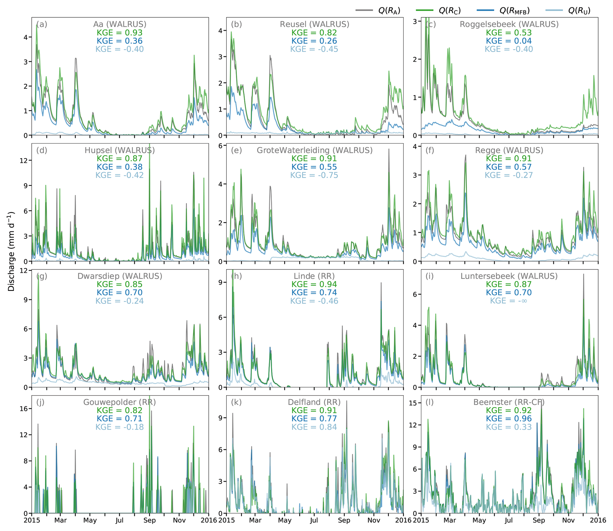
Figure 7 Differences in simulated discharges for the 12 basins (a–l) as a result of the differences between rainfall estimates. The models are run for the period 2009–2018 with the following rainfall products as input: the reference (R_A; grey), the QPE corrected with the CARROTS factors (R_C; green), the MFB-adjusted QPE (R_MFB; dark blue) and the unadjusted radar rainfall estimates (R_U; light blue). Only the simulated discharges for 2015 are shown here for clarity; the KGE is based on all years.

The model runs using R_MFB as input significantly improve the simulated discharges, compared to the runs with R_U. Nevertheless, the model runs still strongly underestimate the simulated discharges compared to those from the reference runs for the catchments in the south and east of the country (Fig. 7a–f). This is particularly noticeable for the catchments Reusel (KGE = 0.26) and Roggelsebeek (KGE = 0.04). The spatial uniformity of the MFB factors is identified as the cause of these effects because the MFB method can not correct for the sources of errors leading to the biased QPE in space. This already led to clear underestimations in the annual rainfall sums for these regions (Fig. 6).

The CARROTS QPE outperforms R_MFB when this product is used as input for the 12 rainfall-runoff models. This is not exclusively the case for the six catchments in the east and south of the country (Fig. 7a–f), but also for the other polder and catchment areas. The exception to this is the Beemster polder. The Beemster is mostly fed by upward seepage, leading to a more predictable baseflow for all models runs. In addition, the catchment is located close to an automatic weather station and is located between both operational radars, which makes the MFB adjustment more beneficial for this region. The difference in performance between the hydrological model simulations is small, with a KGE of 0.92 (using R_C) versus 0.96 for R_MFB, as compared to the reference run.

3.4 Sensitivity analysis

The use of a different moving window size hardly influences the CARROTS factors for moving window sizes of 2 weeks or longer, but this does not hold for moving window sizes of a day or, to a lesser extent, 1 week (Fig. 8a). The factor derived with a moving window size of 1 d fluctuates heavily from day to day. This suggests that the adjustment factor is still quite sensitive to individual events in the 10-year period, when a moving window size of 7 d or shorter is used. Moving window sizes of more than a month (6 weeks and 2 months were tested here) lead to similar CARROTS factors as with a 1-month (31 d) moving window size but somewhat more smoothed. A similar effect likely takes place for a seasonal (3-month) moving window. For larger moving window sizes (half a year to a year, for instance), we expect that the seasonality in the factor is lost and that an average correction factor remains.

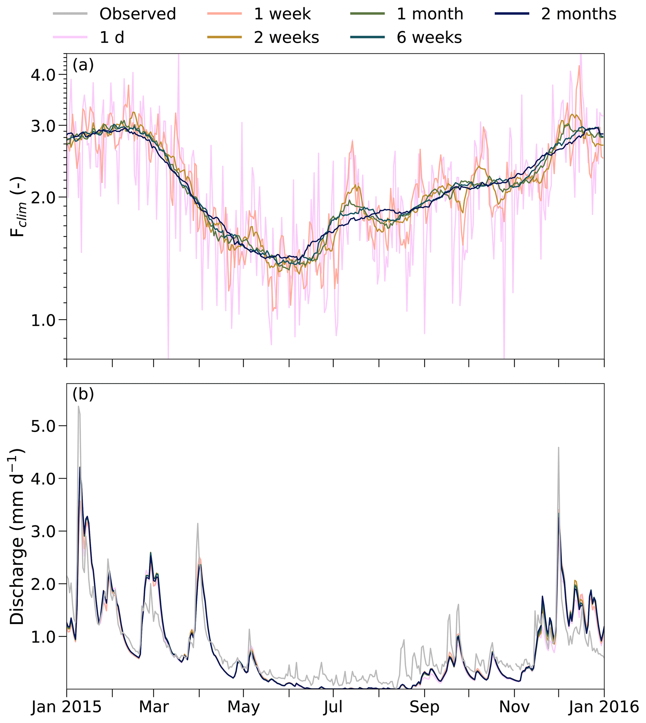
Figure 8 Sensitivity of the CARROTS factor derivation to the moving window size. (a) The adjustment factors for the Aa catchment for six different moving window sizes. The moving window size of 31 d was used in the methodology of this study. (b) The effect of the six moving window sizes in (a) on the simulated discharges for the Aa. Similar to Fig. 7, the CARROTS factors were derived, and discharge was simulated for the full period (2009–2018), but only 2015 is shown here. The grey line indicates the observed discharge.

In contrast to this, the differences between these six sets of CARROTS factors (Fig. 8a) lead to minimal variations in the simulated discharges for the Aa catchment when these factors are used to adjust the input QPE (Fig. 8b). Differences in timing and magnitude (0.2–0.3 mm d⁻¹) are visible during peaks and recessions, for instance in early April. However, these are small compared to the differences between the model runs with R_C and R_MFB (Fig. 7). However, the use of a window size of 1 d or, to a lesser extent, of a week clearly leads to more fluctuations in the CARROTS factor (Fig. 8a) and can therefore influence the rainfall estimation for individual events (and the factor will also be influenced by these individual events). For quickly responding catchments and urban catchments, this could still lead to different results. In conclusion, a 31 d smoothing of the climatological adjustment factor is warranted.

In addition, leaving individual years out of the 10-year archive has a limited impact on the CARROTS factors (see also the vertical bars in Fig. 4c). Similar to the aforementioned results for the moving window size analysis, it leads to hardly any variations in the simulated discharges for the Aa catchment (not shown here). This suggests that the 10-year archive length was sufficiently long for the factor derivation.

4 Discussion

In this study, we introduced the CARROTS method to derive adjustment factors that reduce the bias in radar rainfall estimates. We derived these factors using 10 years of 5 min radar and reference rainfall data for the Netherlands. The method and resulting QPE product outperformed the mean field bias (MFB) adjustment that is used operationally in the Netherlands for catchments in the east and south of the country. When the QPE products were used as input for hydrological model runs, the method outperformed the MFB-adjustment method for all but one basin.

The main difference that distinguishes the CARROTS method from the MFB adjustment is the presence of a high-density network of (manual) rain gauges in the reference dataset, a dataset that is not available in real time. This allows for spatial adjustments. Overeem et al. (2009b) demonstrate that this reference dataset mostly depends on the daily spatial adjustments from the manual rain gauges, while the higher frequency MFB adjustment based on the automatic gauges plays a smaller role in the adjustments of this reference product. According to Saltikoff et al. (2019), at least 40 countries have an archive of historical radar data for a period of 10 years or more. The proposed CARROTS method is potentially valuable for these countries, especially when the density of their network of automatic rain gauges is, similar to the Netherlands, significantly smaller than the total network of rain gauges. An additional advantage of the method is the real-time availability of the correction factors, which is independent of the timeliness of the rain gauge data.

MFB adjustment of radar rainfall fields is still the most frequently applied adjustment method (Holleman, 2007; Harrison et al., 2009; Thorndahl et al., 2014; Goudenhoofdt and Delobbe, 2016). The results indicate that this choice may be reconsidered for hydrological applications in the Netherlands, especially further away from the radar and in the case that a country-wide or large-region adjustment factor is applied. This could also hold for other regions, especially mountainous regions, where the uniformity of the MFB-adjustment factor is likely not sufficient to correct for all orography-related errors (Borga et al., 2000; Gabella et al., 2000; Anagnostou et al., 2010). More regionalized MFB adjustments are possible but depend on the density and availability of the automatic gauge stations.

However, the proposed CARROTS method has to be recalculated for every change in the radar setup, calibration, additional post-processing steps (e.g., VPR corrections;  Hazenberg et al., 2013) or final composite generation algorithm. For instance, including a new radar in the composite would require a recalculation of the adjustment factors, thereby assuming the presence of an archive of the new composite product. This could potentially limit the usefulness of the proposed method. As mentioned in Sect. 2.1, the replacement of both Dutch radars by dual-polarization radars in combination with the replacement of the radar at location De Bilt by the location Herwijnen (Fig. 1) between September 2016 and January 2017 only had a limited impact on the operational products and thereby on the CARROTS derivation. The operational products are not yet (fully) making use of the dual-polarization potential. We expect that the factors will have to be recalculated as soon as the additional information from the dual-polarization radars is used to improve the products or when, e.g., the German and Belgian radars close to the Dutch border are added to the composite.

That CARROTS is relatively insensitive to such minor changes in the composite or the year-to-year variability of rainfall is likely a result of the 10-year archive that has been used. The sensitivity analysis in Sect. 3.4 has shown that leaving individual years out of the archive hardly influences the CARROTS factors. Nevertheless, based on the current analysis, we cannot conclude what the minimum number of years in the archive has to be to obtain stable CARROTS factors that are similar to the factors derived in this study. This is a recommendation for future research. In the case of a new radar QPE product, it is also recommended to recalculate the archive (if possible), to make sure new CARROTS factors can be derived.

Although the results are promising, this method is not expected and meant to outperform more advanced spatial QPE adjustment methods, such as geostatistical and Bayesian merging methods (for an overview of methods and their limitations, see Ochoa-Rodriguez et al., 2019). A major advantage of these methods is the real-time derivation of spatial adjustment factors, in contrast to the proposed method in this study, which was solely based on historical data. The MFB-adjustment factors can also be derived in near real time but are uniform in space, which can explain the worse performance as compared to the proposed method in this study. A possible disadvantage of these real-time methods (MFB, geostatistical and Bayesian merging) is the dependency on the timely availability of rain gauge data, which is not the case for CARROTS. Altogether, we consider the proposed climatological radar rainfall adjustment method to be a benchmark for the development and testing of operational radar QPE adjustment techniques.

Another possible option would be to combine the CARROTS method with the real-time application of the MFB adjustment; i.e., CARROTS is applied, and the resulting QPE is then adjusted with real-time MFB-adjustment factors. This would allow for real-time temporal corrections of the QPE, without the need for a high density of rain gauges in real time, while the corrections in space are based on the (historical) CARROTS factors.

As mentioned in the previous paragraph, the climatological adjustment factor is not calculated for the current meteorological conditions and resulting QPE errors, which could lead to considerable errors during extreme events. Nonetheless, this is also the case for the MFB-adjustment technique (Schleiss et al., 2020). The absolute errors for the 10 highest daily sums in this study for the Aa and Hupsel Brook catchments (one of the largest and the smallest catchment in the study) are similar for the MFB and climatological adjustment methods, with on average a 20 % difference with the reference (this would have been 50 % to 60 % without corrections). In most of these events, both R_C and R_MFB underestimated the true rainfall amount. However, for a small number of these top 10 events, the QPE products overestimated the true rainfall amount. This occurred more frequently with CARROTS (25 % of the cases) than with the MFB adjustment (15 % of the cases). Note that for individual events in these 20 extremes, the errors can still reach 48 % for the QPE adjusted with CARROTS and 64 % for the MFB-adjusted QPE. A way to better correct for biases during extreme events could be to derive either different Z–R relationships, depending on the type of rainfall, or dBZ-dependent correction factors, which could be derived in a similar way to the CARROTS derivation method. Whether this works or not for extreme events depends on the number of such events in the available historical dataset.

Finally, the CARROTS factors were derived with the reference rainfall data for the Netherlands. The same data were used as reference in this study. Although the use of the same data as training and validation set is suboptimal, leaving out individual years has had a limited impact on the estimated adjustment factors and the resulting QPE and discharge simulations (see also the vertical bars in Fig. 4c). Note, however, that in basins with a large number of manual rain gauges, but where automatic rain gauges are not nearby, the CARROTS results will likely be closer to the reference than the MFB-adjusted simulations. Although this is warranted for the CARROTS method, it can partly explain why the method works better for some catchments than others.

5 Conclusions

A known issue of radar quantitative precipitation estimations (QPE) is the significant biases with respect to the true rainfall amounts. For this reason, radar QPE adjustments are needed for operational use in hydrometeorological (forecasting) models. Current QPE adjustment methods depend on the timely availability of quality-controlled rain gauge observations from dense networks. This especially applies to methods that correct for the spatial variability in the QPE errors. To overcome this issue and to provide a benchmark for future QPE algorithm development, we have presented CARROTS (Climatology-based Adjustments for Radar Rainfall in an OperaTional Setting), a set of gridded climatological adjustment factors for every day of the year. The factors were based on a historical set of 10 years of 5 min radar rainfall data and a reference dataset for the Netherlands. The climatological adjustment factors were compared with the mean field bias (MFB) adjustment factors, which are used operationally in the Netherlands. For the period 2009–2018, daily and sub-daily rainfall estimates with both the MFB-adjusted and CARROTS-adjusted QPE were validated against the reference rainfall for the land surface area of the Netherlands. In order to provide a hydrometeorological testbed, the estimated annual rainfall sums and the effect of the adjusted QPE products on simulated discharges with the rainfall-runoff models for 12 Dutch basins were validated for both adjustment methods.

The CARROTS factors show clear spatial and temporal patterns, with higher adjustment factors towards the edges of the radar domain. This is caused by larger QPE errors further away from the radars. The factors are also higher from December through March than in other seasons. This is likely a result of sampling above the melting layer during these months, which causes higher underestimations in the unadjusted radar rainfall product.

On average for the Netherlands, the MFB-adjusted QPE outperforms the CARROTS-corrected QPE. Although the MFB factors are based on the current over- or underestimations in the QPE, the factor is spatially uniform and does not correct for spatial errors. This directly impacts the adjusted QPE when the QPE products are tested for the 12 Dutch basins. The MFB-adjusted QPE leads to annual rainfall sums that still underestimate those of the reference for the catchments in the east and south of the country (towards the edge of the radar domain). This bias is almost absent for the annual rainfall sums after correction with the CARROTS factors (up to 5 % over- and underestimation for the same catchments). For basins closer to radars, this effect decreases, and both adjustment methods perform well.

The effects of both adjustment methods on the QPE are amplified when they are used as input for the rainfall-runoff models of the 12 studied basins. The discharge simulations with the CARROTS QPE outperform those using the MFB-adjusted QPE for all but one basin. For hydrological applications in the Netherlands, these results indicate that the current operational use of a country-wide MFB adjustment may be reconsidered as it often performs worse than the proposed climatological adjustment factor, which can be seen as the minimum benchmark to outperform.

Despite the aforementioned results, the CARROTS method has two main limitations: (1) for every change in the radar setup, the radar calibration, post-processing algorithms or the final composite generation method, the adjustment factors have to be recalculated; (2) the factor is not calculated for the actual meteorological conditions and resulting QPE errors, which could lead to considerable errors during extreme events. Nonetheless, the latter is also the case for the MFB-adjustment technique (Schleiss et al., 2020), even though the MFB factors are derived in real time.

The main advantage of the introduced method is the continuous availability of spatially distributed adjustment factors, due to the independence of timely rain gauge observations. This is beneficial for operational use. In addition, the CARROTS factors are shown to be robust, as the derivation is not found to be sensitive to leaving out individual years or to the moving window used, especially when this window is longer than a week.

Finally, this method is not expected and meant to outperform more advanced spatial QPE adjustment methods (which require data from dense rain gauge networks for robust application), but it can serve as a benchmark for the development and testing of more advanced operational radar QPE adjustment techniques. QPE adjustment methods (including CARROTS) greatly benefit from a denser, frequently available rain gauge network. From that perspective, crowd-sourced personal weather stations have promise for improving radar rainfall products, given their direct surface measurements and dense networks (Vos et al., 2019). This also holds for rain gauge observations from other governmental or third parties, e.g., the water authorities in the Netherlands. Hence, we think that this could further improve radar rainfall products in the near future.

Appendix A: Hourly evaluation of the rainfall sums

Table A1 Country-average fractional standard error (FSE) between the hourly reference rainfall (R_A) and the three QPE products (R_U, R_MFB and R_C) per year for the winter (DJF) and summer (JJA) seasons. The FSE was only calculated for hours in which the country-average rainfall rate was larger than 0.0 mm h⁻¹.

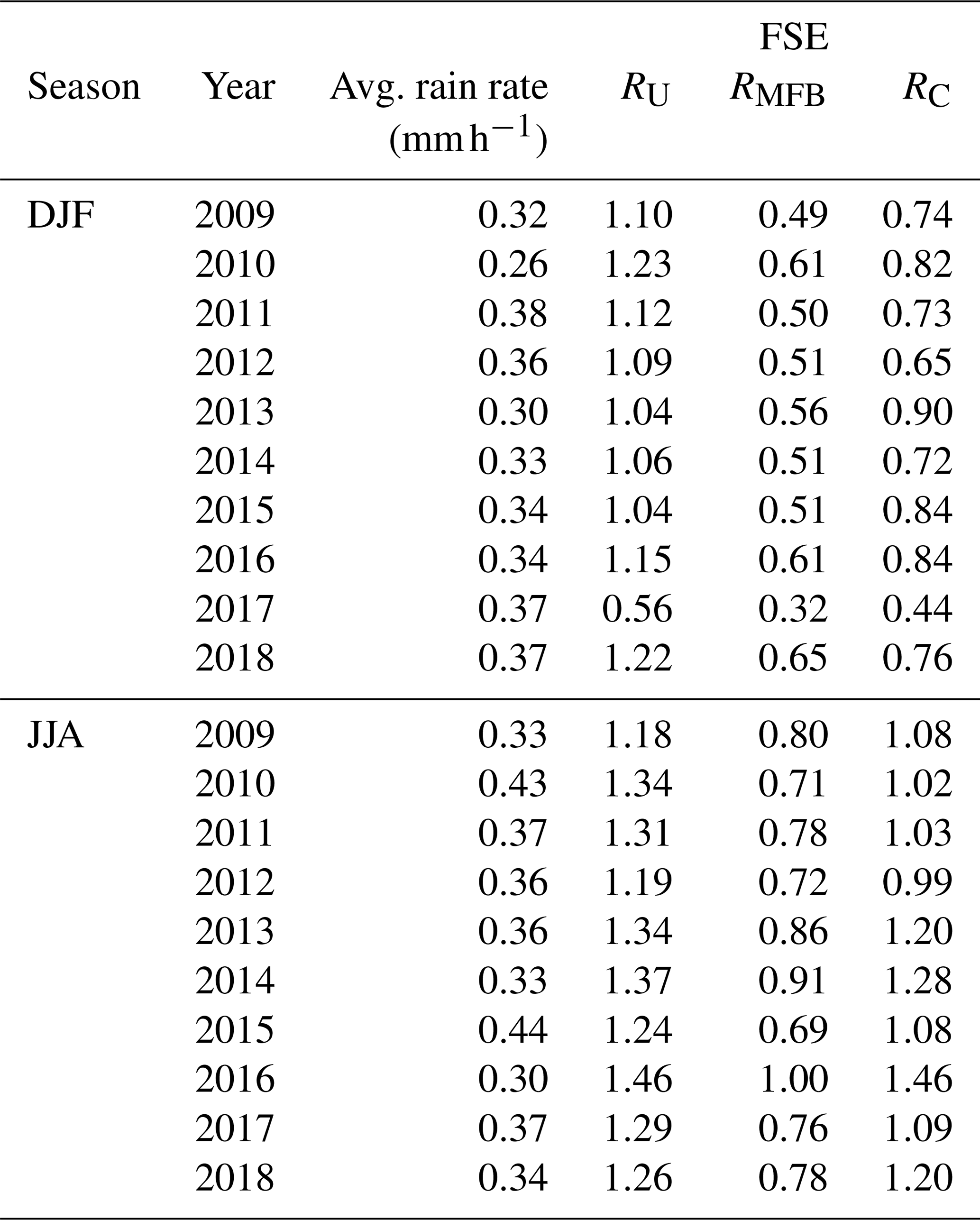
Table A1 shows the country-average FSE between R_A and the three QPE products for every year and the winter and summer seasons. The method to calculate the FSE score is described in Sect. 2.3.